The Gerasimov-Drell-Hearn Sum Rule

Abstract

Sum rules measurements involving the spin structure of the nucleon like those due to Bjorken, Ellis and Jaffe and the one due to Gerasimov, Drell and Hearn allow to study the structure of strong interactions. At long distance scales in the confinement regime the Gerasimov-Drell-Hearn (GDH) Sum Rule (Eq. (1)) connects static properties of the nucleon - like the anomalous magnetic moment and the nucleon mass - with the difference of spin dependent doubly polarized total absorption cross sections of real photons. Hence, the full spin-dependent excitation spectrum of the nucleon is being related to its static properties. The sum rule has not been investigated experimentally until recently. Now, for the first time this fundamental sum rule is verified by the GDH-Collaboration with circularly polarized real photons and longitudinally polarized nucleons at the two accelerators Elsa and Mami. The investigation of the response of the proton as well as of the neutron allows to perform an isospin decomposition. Further investigations with real photons are scheduled at Slac, JLab, Spring-8, Legs and Graal. The integral (sum) of the GDH Sum Rule can be generalized to the case of virtual photons. This allows to establish a $Q^{2}$ dependency and to study the transition to the perturbative regime of QCD. Ultimately, the GDH Sum Rule can be related to the Bjorken and the Ellis-Jaffe Sum Rule. This transition is the subject of several experiments e.g. at JLab for the resonance region and of the Hermes experiment at Desy for higher $Q^{2}$.

This contribution covers the status of theory concerning the GDH Sum Rule as well as the experimental approaches and their results for the absorption of real and virtual photons. We point out that the so-called No-Subtraction hypothesis, often considered the weakest part of the derivation of the GDH Sum Rule, in fact follows from unitarity and does not impair the fundamental character of the GDH Sum Rule. The experimental data verify the GDH Sum Rule for the proton at the level of 8 % including the systematic uncertainties from extrapolations to unmeasured energy regions. For the GDH Sum Rule on the neutron and the isovector case we find unexpected contributions at photon energies above 1 GeV.

$$\Large\boxed{\boxed{~{}\int\limits_{0}^{\infty}\frac{d\nu}{\nu}\left[\sigma_{3/2}(\nu)-\sigma_{1/2}(\nu)\right]=\frac{2\pi^{2}\alpha}{m^{2}}\kappa^{2}~{}}}$$ (1)

1 Introduction

Understanding the spin structure of the nucleon is at the heart of present nuclear and particle physics activities. Of particular interest are sum rules which connect information from all energies to fundamentals of our current view of nature’s laws. The Gerasimov-Drell-Hearn (GDH) sum rule is an excellent example of a whole class of dispersive sum rules which are consequences of general principles. They can be used to test these fundamental principles and thus probe deep mysteries of nature. Also, these sum rules provide a vehicle to access new experimental observables and to study the physics of strongly interacting systems in refined detail.

The Gerasimov-Drell-Hearn sum rule was established in the second half of the 1960ies. The two independent derivations presented by Sergei B. Gerasimov [1] and by Sidney D. Drell and Anthony C. Hearn [2] both appeared in 1966 in English language, while Gerasimov’s original publication [3] was available in Russian language already in 1965. We owe this historic detail today’s naming sequence for the sum rule: Gerasimov-Drell-Hearn sum rule. In fact, initially the sum rule was called Drell-Hearn-Gerasimov sum rule. The change in sequence was adopted first for the naming of the GDH-Collaboration— the collaboration that finally took the challenge to verify this fundamental sum rule. This sequence is widely accepted today. One might even add two more names to the sum rule: Hosoda and Yamamoto [4] used the current algebra formalism for their derivation also dated 1966.

Figure 1: Citation statistics for the two sum rule derivations of Gerasimov [1] and Drell and Hearn [2] according to Spires.

Fig. 1 shows the citation statistics for the sum rule derivations of Gerasimov [1] and Drell and Hearn [2] according to Spires as a function of time. One observes that until 1990 the interest in the GDH Sum Rule is essentially constant. This hesitant reaction was probably driven by the problem to estimate the experimental feasibility of a verification at that time. For example: Gerasimov rated the sum rule mainly to be of academic interest only, while Hosoda and Yamamoto were convinced that it would be straightforward to test it experimentally. Drell and Hearn, however, state that a test would be a formidable experimental challenge and call for it.

Consequently, the early discussion was centered around questions connected to the validity of the GDH Sum Rule. As an example the title of Ref. [5] might serve: “Drell-Hearn-Gerasimov sum rule: Examples and Counterexamples”. Experimentally, only multipole analyses of unpolarized single pion photoproduction data were possible, from which — in an indirect fashion — estimates of the contribution from low-lying resonances to the GDH integral were extracted.

Albeit by then about a quarter of a century old, in the early 1990ies the GDH sum rule still lacked a direct experimental check, since a doubly polarized photoabsorption measurement is needed covering a wide energy range. This challenge had never been taken up so far. The GDH-Collaboration was established to bring together polarized sources and polarized targets as well as detectors suited to measure total photoabsorption cross sections at two electron accelerators — Elsa (Bonn) and Mami (Mainz). The collaboration has about 60 members coming from 16 institutions from all over Europe, Japan and Russia.

The renewed interest in the GDH Sum Rule arose not only due to the availability of experimental techniques but was also stimulated by the apparent failure of the Ellis-Jaffe sum rule [6] as reported in polarized deep inelastic scattering experiments at Slac [7] and Cern [8]. Although the Ellis-Jaffe sum rule cannot be regarded to be quite as fundamental as the GDH Sum Rule it gave rise to the so-called “spin crisis” in the late 1980ies. It became clear that further precision tests were needed to improve our understanding of the spin structure of the nucleon.

In 1998 the GDH-Collaboration at Mami provided the first direct information on the helicity structure as probed by real photons. The GDH Sum Rule for the proton was verified in 2001 together with the data taken at Elsa by the GDH-Collaboration [9, 10]. The data taking of the GDH-Collaboration is completed since 2003.

In the aftermath of the efforts to determine the helicity structure with real photons also experiments at JLab in Hall A and with the Clas detector and at Desy with the Hermes detector help to identify the spin structure of the nucleon for intermediate photon virtualities. Besides the direct verification of the GDH Sum Rule a wealth of new data is now available to disentangle the involved structure of the nucleon aided by polarization observables. For a recent reviews on this subject see for example [11, 12].

This review in detail discusses the status of theoretical considerations concerning the GDH Sum Rule at the real photon point including a survey of problems with the interpretation of the sum rule and of possible modifications. Also, the generalizations of the GDH Sum Rule to finite photon virtuality and the connection to other sum rules are outlined.

On the experimental side experiments with a connection to the GDH Sum Rule are addressed. Virtues of future experiments and their chances to improve the current understanding of the GDH Sum Rule are also discussed. The experiments of the GDH-Collaboration will receive the most attention as these measurements are – so far – the only ones that have lead to a direct test of the GDH Sum Rule with real photons.

2 The GDH Sum Rule for real photons

As already mentioned in the introduction, there is more than one method to derive the Gerasimov-Drell-Hearn sum rule: Gerasimov [1] as well as Drell and Hearn [2] used a dispersion theoretic approach. Hosoda and Yamamoto [4] on the other hand used the current algebra formalism for their derivation of the very same sum rule. And there is yet another way: In 1972, Dicus and Palmer [13] presented a derivation of the GDH Sum Rule from the algebra of currents on the light-cone.

In the following all three of these derivations will be discussed with their main aspects. We present the dispersion theoretic derivation in most detail as it is very instructive. Also, the dispersion theoretic approach is the most illustrative in identifying where the fundamental principles actually enter the derivation.

We will show that the dispersion theoretic derivation of the GDH Sum Rule is possible without the restriction to lowest non-vanishing order in electromagnetic coupling. While the low energy theorems indeed were shown only in low orders of coupling all other steps of the dispersion theoretic derivation hold without this limitation; especially the validity of the No-Subtraction hypothesis is guaranteed only without this restriction. Concerning the low energy theorems we argue that the magnetic moment of the nucleon in low electromagnetic order may deviate only insignificantly from the measured one, so that in view of the experimental errors of the verification of the GDH Sum Rule the limitation to low orders can be neglected here. This way we overcome a discussion of the validity of the No-Subtraction hypothesis which so far has resisted attempts of an interpretation in terms of the internal dynamics of the nucleon.

2.1 Dispersion theoretic derivation

The dispersion theoretic derivation exclusively relies on the following assumptions:

• Lorentz invariance

• Gauge invariance

• Crossing symmetry

• Rotational invariance

• Causality and

• Unitarity

All our modern relativistic quantum field theories rely on these principles. Hence a verification of the GDH sum rule provides a vital cross check of the foundations of modern physics.

By means of crossing symmetry, rotational invariance and gauge invariance the Compton forward scattering amplitude takes a very simple form with analytical behavior. Causality leads to the analytic continuation of the Compton forward scattering to complex values of the photon energy which leads to the Kramers-Kronig dispersion relation. The Kramers-Kronig dispersion relation connects the static limit with the integral of the elastic scattering amplitude of all energies. Elastic scattering (here, Compton scattering) is connected to the total cross section by unitarity, the optical theorem. Finally, the elastic scattering is connected to static properties of the nucleon by means of low-energy limits following from gauge and Lorentz invariance and crossing symmetry. In the following we will outline this derivation in detail.

2.1.1 Spin dependent Compton forward scattering amplitude

The elastic scattering of light on elementary particles has been a key subject in the course of the formulation of particle physics especially for the electromagnetic force. Compton scattering is the cornerstone also of the derivation of the GDH Sum Rule.

To discuss the spin content of general Compton scattering off spin-1/2 systems with real or virtual photons one uses helicity amplitudes [14] by choosing appropriate photon and nucleon polarization states. We denote the helicity amplitudes by $M_{\lambda^{\prime},\nu^{\prime};\lambda,\nu}$ with $\lambda,\lambda^{\prime}=\pm 1$ and $\nu,\nu^{\prime}=\pm 1/2$. These 16 amplitudes depend on the Lorentz-invariant Mandelstam variables s and t. By parity invariance $M_{-\lambda^{\prime},-\nu;-\lambda,-\nu}=(-1)^{\lambda-\nu-\lambda^{\prime}+\nu^{\prime}}M_{\lambda^{\prime},\nu^{\prime};\lambda,\nu}$ only 8 amplitudes are independent. Time-reversal invariance $M_{\lambda^{\prime},\nu;\lambda,\nu}=(-1)^{\lambda-\nu-\lambda^{\prime}+\nu^{\prime}}M_{\lambda^{\prime},\nu^{\prime};\lambda,\nu}$ reduces the number of amplitudes to 6 [15] for which one may take

$$\phi_{1}=M_{1\frac{1}{2},1\frac{1}{2}}\quad \quad\phi_{2}=M_{-1-\frac{1}{2},1\frac{1}{2}}\quad \quad\phi_{3}=M_{-1\frac{1}{2},1\frac{1}{2}}$$

$$\phi_{4}=M_{1-\frac{1}{2},1\frac{1}{2}}\quad \quad\phi_{5}=M_{1-\frac{1}{2},1-\frac{1}{2}}\quad \quad\phi_{6}=M_{-1\frac{1}{2},1-\frac{1}{2}}$$ (2)

By angular momentum conservation in forward direction only $\phi_{1}$ and $\phi_{5}$ can contribute.

The requirement of C, P and T invariance is somewhat cumbersome and indeed if we restrict the discussion to real photons we can get over it and instead use assumptions that are essential to other parts of the derivation as well: We use the special gauge useful for real photons with the time component $\mathcal{A}^{0}=0$ of the photon field $\mathcal{A}$. Compton scattering is symmetric under the exchange of the in- and outgoing photons ($\vec{k_{1}}\leftrightarrow-\vec{k_{2}}$ and $\vec{\epsilon_{1}}\leftrightarrow\vec{\epsilon_{2}}^{*}$). $\vec{\epsilon}_{1,2}$ and $\vec{k_{1,2}}$ label the initial and the final polarization of the Compton scattered photon and their momenta respectively. This symmetry is called crossing-symmetry and is exact for all orders of electromagnetic coupling. Therefore we have the following crossing properties for the Compton amplitude

$$F(\vec{k_{1}},\vec{\epsilon}_{1},\vec{\epsilon}_{2})=F^{*}(-\vec{k_{2}},\vec{\epsilon_{2}}^{*},\vec{\epsilon_{1}}^{*})\ .$$ (3)

Due to the superposition principle $F$ has to be linear in $\vec{\epsilon_{1}}$ and $\vec{\epsilon_{2}}$. We now restrict the discussion to forward scattering where $\vec{k}\equiv\vec{k_{1}}=\vec{k_{2}}$. In the nucleon rest frame the amplitude $F$ can be written as a linear combination with scalar functions $f_{i}$:

$$F = \left<\chi_{2}^{\dagger}\left|\sum_{i=1}^{5}f_{i}\ K_{i}\right|\chi_{1}\right>$$ (4)

$$= \left<\chi_{2}^{\dagger}\right|f_{1}\ \left(\vec{\epsilon_{2}}^{*}\cdot\vec{\epsilon_{1}}\right)\qquad+$$

$$\qquad f_{2}\ i\vec{\sigma}\left(\vec{\epsilon_{2}}^{*}\times\vec{\epsilon_{1}}\right)\qquad+$$

$$\qquad f_{3}\ \left(\vec{\epsilon_{2}}^{*}\cdot\vec{k}\right)\left(\vec{\epsilon_{1}}\cdot\vec{k}\right)\qquad+$$

$$\qquad f_{4}\ i\vec{\sigma}\left[\vec{\epsilon_{2}}^{*}\left(\vec{\epsilon_{1}}\cdot\vec{k}\right)-\vec{\epsilon_{1}}\left(\vec{\epsilon_{2}}^{*}\cdot\vec{k}\right)\right]\quad+$$

$$\qquad\left.\left.f_{5}\ i\vec{\sigma}\left[\left(\vec{\epsilon_{2}}^{*}\times\vec{k}\right)\left(\vec{\epsilon_{1}}\cdot\vec{k}\right)-\left(\vec{\epsilon_{1}}\times\vec{k}\right)\left(\vec{\epsilon_{2}}^{*}\cdot\vec{k}\right)\right]\qquad\right|\chi_{1}\right>$$

$\vec{\sigma}$ is the vector of Pauli spin matrices and $\chi_{1,2}$ are the initial and final spinors of the nucleon. With the theory of the rotation group one can show that no more linearly independent combinations can be found. The transversality condition for real photons reads $\vec{\epsilon}\cdot\vec{k}=0$ and one observes that only the first two terms contribute. Hence, we can write the forward scattering amplitude $F(\theta=0,\nu)$ with the photon energy $\nu$:

$$F(\theta=0,\nu)=\left<\left.\left.\chi_{2}^{\dagger}\right|\ f_{1}(\nu)\ \vec{\epsilon_{2}}^{*}\cdot\vec{\epsilon_{1}}+f_{2}(\nu)\ i\vec{\sigma}\left(\vec{\epsilon_{2}}^{*}\times\vec{\epsilon_{1}}\right)\ \right|\chi_{1}\right>$$ (5)

The polarization vectors for left and right handed photons are

$$\vec{\epsilon}_{R}=-\frac{1}{\sqrt{2}}(\vec{\epsilon}_{x}+i\vec{\epsilon}_{y})\quad,\qquad\vec{\epsilon}_{L}=+\frac{1}{\sqrt{2}}(\vec{\epsilon}_{x}-i\vec{\epsilon}_{y})$$ (6)

with the z-axis being the direction of motion of the photon. For the two terms of Eq. (5) one obtains the following combinations:

$$\vec{\epsilon}_{2}^{\ \ast}\cdot\vec{\epsilon}_{1}=\left\{\begin{array}[]{r@{\quad:\quad}l}1&\vec{\epsilon}_{1}=\vec{\epsilon}_{2}=\vec{\epsilon}_{R}\\ 1&\vec{\epsilon}_{1}=\vec{\epsilon}_{2}=\vec{\epsilon}_{L}\\ 0&\text{else}\end{array}\right.\quad,$$ (7)

$$\vec{\epsilon}_{2}^{\ \ast}\times\vec{\epsilon}_{1}=\left\{\begin{array}[]{r@{\quad:\quad}l}-i\vec{\epsilon}_{z}&\vec{\epsilon}_{1}=\vec{\epsilon}_{2}=\vec{\epsilon}_{L}\\ +i\vec{\epsilon}_{z}&\vec{\epsilon}_{1}=\vec{\epsilon}_{2}=\vec{\epsilon}_{R}\\ 0&\text{else}\end{array}\right.$$ (8)

We can now compute the Compton amplitude for all possible spin configurations. As it turns out, we only need to distinguish the orientation of nucleon and photon spins in parallel ($3/2$) and anti-parallel ($1/2$):

$$f_{3/2}(\nu)=f_{1}(\nu)-f_{2}(\nu)\quad,\qquad f_{1/2}(\nu)=f_{1}(\nu)+f_{2}(\nu)$$ (9)

$f_{3/2}$ and $f_{1/2}$ can be associated with $\phi_{1}$ and $\phi_{5}$ in Eq. (2).

For the treatment of analyticity in Sec. 2.1.2 however, it is important to work with a set of amplitudes free of kinematic singularities and zeros (KSZF). It is not clear a priori if $f_{1}$ and $f_{2}$ fulfill this requirement. The KSZF invariant amplitudes can be obtained by a rather tedious construction procedure [16]. For their definition one writes the general Compton amplitude like $T={e^{\mu}}^{{}^{*}}_{(\lambda^{\prime})}{e^{\nu}}_{(\lambda)}T_{\mu\nu}$. The tensor $T_{\mu\nu}$ may be expanded with respect to a tensor basis $I^{i}_{\mu\nu}$:

$$T_{\mu\nu}=\sum_{i=1}^{6}A_{i}I^{i}_{\mu\nu}$$ (10)

where the KSZF invariant amplitudes $A_{i}$ depend on the Lorentz invariant variables s, t and u. The explicit construction leads to the following relation of the $A_{i}$ to the $f_{1,2}$ of Eq. (5):

$$f_{1} = \frac{\nu^{2}m}{4\pi}\left[mA_{2}+2A_{3}\right]$$

$$f_{2} = \frac{\nu^{2}m}{4\pi}A_{4}$$ (11)

with the nucleon mass $m$. Due to the work of Ref. [16] we see that also $f_{1},f_{2}$ and even $f_{2}/\nu$ are free of kinematic zeros and singularities. This is important as we will need the analyticity of these functions of the photon energy on the real axis in Sec. 2.1.2.
In conclusion, we have shown that the forward Compton scattering takes the very simple form of Eq. (5) with only two amplitudes that have the mathematical properties we will need in the following section.

2.1.2 Kramers-Kronig dispersion relation

Causality applied to scattering implies that the scattered wave $\psi_{\text{scatt}}(z,t)$ at time $t$ can be influenced by the incoming wave $\psi_{\text{inc}}(z^{\prime},t^{\prime})$ only at times $t^{\prime}$ prior to $t$ with $z=z^{\prime}$. The scattered wave depends linearly on the incoming wave:

$$\psi_{\text{scatt}}(z,t)=\int\limits_{-\infty}^{\infty}dt^{\prime}\ K(z^{\prime}-z,t-t^{\prime})\ \psi_{\text{inc}}(z^{\prime},t^{\prime})\qquad\text{with }K(\zeta,\tau)=0\text{ for }\tau<\zeta.$$ (12)

In the context of wave packets we can assume without loss of generality that $\psi_{\text{inc}}(z,t)=0$ for $z>t$. Then, due to the characteristics of $K(\zeta,\tau)$, the same also holds for $\psi_{\text{scatt}}$. We can now obtain the scattering amplitude as a function of the energy $\nu$ or frequency $\omega=\nu/2\pi$ by performing a Fourier transform of $\psi_{\text{scatt}}(z,t)$:

$$f_{\text{scatt}}(\omega)=\frac{1}{\sqrt{2\pi}}\int\limits_{-\infty}^{z}dt\ \psi_{\text{scatt}}(z,t)\ e^{-i\omega(t-z)}$$ (13)

By taking $z=0$ it is easy to demonstrate that $f_{\text{scatt}}$ can be extended analytically into the full upper half of the complex plane:

$$f_{\text{scatt}}(\omega+i\left|\gamma\right|)=\frac{1}{\sqrt{2\pi}}\int\limits_{-\infty}^{0}dt\ \psi_{\text{scatt}}(0,t)\exp(-i\omega t-\left|\gamma\right|\left|t\right|)$$ (14)

Also, we have to keep in mind that $\psi_{\text{scatt}}$ is bounded which is guaranteed by unitarity. For wave packets we have $t\to-\infty:\psi_{\text{scatt}}(z,t)\to 0$. This in turn tells us that for a given $\omega$ one can find a local neighborhood of $\omega$ where $f_{\text{scatt}}$ can be continued into the lower half of the complex plane. It shall be noted that poles that stem for nucleon resonances do not lie on the real axis but rather along the real axis — with our conventions here in the lower half of the complex plane.

Admittedly, the above motivation of the analyticity of the Compton forward scattering is based on ideas of classical electrodynamics. A derivation of the same can also be done in terms of quantum fields [17]. Here causality implies the vanishing of the commutator of two field operators $\phi(x)$ and $\phi(x^{\prime})$ if $x-x^{\prime}$ is space-like. Later Goldberger was able to generalize the argument leading to the derivation of the Kramers-Kronig dispersion relation without the use of perturbation theory [18].

We are now in the position to apply Cauchy’s integral formula:

$$f(\nu)=\frac{1}{2\pi i}\oint\limits_{\cal C}d\nu^{\prime}\frac{f(\nu^{\prime})}{\nu^{\prime}-\nu}$$ (15)

We choose the path $\cal C$ as depicted in Fig. 2 where the integral is to be taken counter-clockwise. $K_{+}(0,\infty)$ is the half-circle at infinity in the upper half of the complex plane and $K_{-}(\nu,\varepsilon)$ a small half circle around $\nu$ of radius $\varepsilon$ in the lower half of the complex plane with the center $\nu$ on the real axis.

Figure 2: Path of integration for Cauchy’s integral formula applied to the forward scattering amplitude

We can now evaluate the individual contributions from the segments of the integration path:

$$f(\nu) = \frac{1}{2\pi i}\;{\cal P}\int\limits_{-\infty}^{\infty}d\nu^{\prime}\frac{f(\nu^{\prime})}{\nu^{\prime}-\nu}$$

$$+\ \frac{1}{2\pi i}\int\limits_{K_{+}(0,\infty)}d\nu^{\prime}\frac{f(\nu^{\prime})}{\nu^{\prime}-\nu}\ +\ \lim_{\varepsilon\to 0}\ \frac{1}{2\pi i}\int\limits_{K_{-}(\nu,\varepsilon)}d\nu^{\prime}\frac{f(\nu^{\prime})}{\nu^{\prime}-\nu}$$

with the Cauchy principle value

$$\;{\cal P}\int_{-\infty}^{\infty}\equiv\lim_{\varepsilon\to 0}\int_{-\infty}^{\nu-\varepsilon}+\int_{\nu+\varepsilon}^{\infty}\ .$$ (17)

The integral for $K_{-}(\nu,\varepsilon)$ is simply half the residue we would get for the full circle: $\frac{1}{2}f(\nu)$. We assume that the integral along the path $K_{+}(0,\infty)$ vanishes which is called the No-Subtraction hypothesis (see Sec. 2.4.3). One then obtains

$$f(\nu)=\frac{1}{\pi i}\ {\cal P}\int\limits_{-\infty}^{+\infty}d\nu^{\prime}\frac{f(\nu^{\prime})}{\nu^{\prime}-\nu}\ .$$ (18)

Recall the crossing properties of Compton scattering mentioned in Sec. 2.1.1. Applied to $F,f_{1},f_{2}$ and $f_{2}/\nu$ we obtain

$$F(\theta=0,-\nu)=F^{*}(\theta=0,\nu)\ ,\quad f_{1}(-\nu)=f_{1}^{*}(\nu)\ ,\quad f_{2}(-\nu)=-f_{2}^{*}(\nu)\ ,\quad\frac{f_{2}(-\nu)}{-\nu}=\frac{f_{2}^{*}(\nu)}{\nu}$$ (19)

As we will use Eq. (18) only for $f_{1}$ and $f_{2}/\nu$ and not for $f_{2}$ we can continue with the crossing relation for $f:f(-\nu)=f^{*}(\nu)$. We can now write Eq. (18) as:

$$f(\nu)=\frac{1}{\pi i}\ {\cal P}\int\limits_{0}^{+\infty}d\nu^{\prime}\left(\frac{f(\nu^{\prime})}{\nu^{\prime}-\nu}+\frac{f^{*}(\nu^{\prime})}{-\nu^{\prime}-\nu}\right)$$ (20)

Considering the real part only, this further simplifies to the famous Kramers-Kronig dispersion relation:

$$\text{Re}\,f(\nu)=\frac{2}{\pi}\ {\cal P}\int\limits_{0}^{\infty}\,d\nu^{\prime}\,\nu^{\prime}\ \frac{\text{Im}\;f(\nu^{\prime})}{\nu^{\prime 2}-\nu^{2}}$$ (21)

2.1.3 Optical theorem

The optical theorem can be derived from probability current conservation which is also called unitarity. It connects the elastic forward amplitude to the total cross section:

$$\text{Im}\;f(\nu)=\frac{\nu}{4\pi}\sigma$$ (22)

For the amplitudes $f_{1,2}$ as defined in Eq. (5) and (11) one obtains

$$\text{Im }f_{1}(\nu) = \frac{\nu}{8\pi}\left[\sigma_{1/2}(\nu)+\sigma_{3/2}(\nu)\right]=\frac{\nu}{4\pi}\sigma_{T}(\nu)\ ,$$ (23)

$$\text{Im }\frac{f_{2}(\nu)}{\nu} = \frac{1}{8\pi}\left[\sigma_{1/2}(\nu)-\sigma_{3/2}(\nu)\right]=\frac{1}{4\pi}\sigma_{TT}(\nu)\ .$$ (24)

For the transverse polarization of the photon the subscripts of the total cross sections $\sigma_{3/2}$ and $\sigma_{1/2}$ denote the total helicity of the photon-nucleon system in the nucleon rest frame with respect to the center of mass momentum. The symbols $\sigma_{TT}$ and $\sigma_{T}$ are commonly used in electron scattering or better to say virtual Compton scattering (see Sec. 3).

Here, it is important to understand that the optical theorem is a statement for the total cross section including both elastic and inelastic contributions: $\sigma=\sigma_{\text{elast}}+\sigma_{\text{inel}}$. Actually a sizable fraction of text books get it wrong and claim the theorem relates the elastic forward scattering to the inelastic part of the cross section only. For the special case of photon scattering the optical theorem relates the imaginary part of the Compton forward scattering amplitude to the total cross section for photon scattering — that is photoabsorption and Compton scattering.

However, if one considers the Compton forward scattering amplitude only up to the lowest non-trivial order in electromagnetic coupling

$$f_{\text{low}}=i\ \frac{e^{2}}{16\pi M}\,\epsilon_{\mu}^{*}\epsilon_{\nu}\int\!d^{4}x\,e^{ik\cdot x}\sum\limits_{X_{\text{had}}}\left<p_{2},s_{2}\left|{J^{\mu}(x)\left|X_{\text{had}}\right>\left<X_{\text{had}}\right|J^{\nu}(0)}\right|p_{1},s_{1}\right>$$ (25)

with the sum over purely hadronic intermediate states $X_{\text{had}}$ only the optical theorem instead reads

$$\text{Im}\;f_{\text{low}}(\nu)=\frac{\nu}{4\pi}\sigma_{\gamma\text{-abs}}$$ (26)

with $\sigma_{\gamma\text{-abs}}$ denoting the photoabsorption cross section only. $J^{\mu}$ is the electromagnetic current of the photon field, $p_{1,2}$ are the initial and final nucleon four-momenta, $s_{1,2}$ the spins. So, to lowest non-vanishing order the optical theorem relates the elastic forward Compton scattering amplitude to the photoabsorption cross section only. It can be proven rigorously that the optical theorem even holds for all orders of coupling individually.

In the language of Feynman diagrams the optical theorem and the question of inclusion of elastic processes in the cross section can be understood graphically in terms of cutting through the diagram for the amplitude of the elastic process:

$${\Large\text{Im}_{\theta=0}}\left(\quad\ \ \begin{minipage}{100.0pt} \begin{picture}(100.0,62.0)\begin{picture}(100.0,62.0)\immediate\ignorespaces\immediate\ignorespaces\immediate\ignorespaces\immediate\ignorespaces\immediate\ignorespaces{\immediate\immediate}\put(0.0,0.0){{\f@ynmf:fd\char 1\relax}}\ignorespaces\immediate\ignorespaces\immediate\ignorespaces\immediate\ignorespaces\immediate\ignorespaces\immediate\ignorespaces\immediate\ignorespaces\immediate\ignorespaces\immediate\ignorespaces\immediate\ignorespaces\immediate\ignorespaces\immediate\ignorespaces\immediate\ignorespaces\immediate\ignorespaces\immediate\ignorespaces\immediate\ignorespaces\immediate\ignorespaces\immediate\ignorespaces\immediate\ignorespaces\immediate\ignorespaces\immediate\ignorespaces\immediate\ignorespaces\immediate\ignorespaces\immediate\ignorespaces\immediate\ignorespaces \immediate\ignorespaces{\put(49.98672,31.01585){\makebox(0.0,0.0)[c]{{\Large\bf X}}} \put(5.18552,-3.73257){\makebox(0.0,0.0)[rt]{n,p}} \put(5.18552,65.76433){\makebox(0.0,0.0)[rb]{$\gamma$}} \put(94.78798,-3.73257){\makebox(0.0,0.0)[lt]{n,p}} \put(94.78798,65.76433){\makebox(0.0,0.0)[lb]{$\gamma$}} \put(49.98676,68.12209){\makebox(0.0,0.0)[b]{\scriptsize cut}} }\end{picture} \end{picture} \end{minipage}\quad\ \ \right)\quad=\quad\left|\quad\begin{minipage}{100.0pt} \begin{picture}(100.0,62.0)\begin{picture}(100.0,62.0)\immediate\ignorespaces\immediate\ignorespaces\immediate\ignorespaces\immediate\ignorespaces\immediate\ignorespaces{\immediate\immediate}\put(0.0,0.0){{\f@ynmf:fd\char 2\relax}}\ignorespaces\immediate\ignorespaces\immediate\ignorespaces\immediate\ignorespaces\immediate\ignorespaces\immediate\ignorespaces\immediate\ignorespaces\immediate\ignorespaces\immediate\ignorespaces\immediate\ignorespaces\immediate\ignorespaces\immediate\ignorespaces\immediate\ignorespaces\immediate\ignorespaces\immediate\ignorespaces\immediate\ignorespaces\immediate\ignorespaces\immediate\ignorespaces\immediate\ignorespaces\immediate\ignorespaces\immediate\ignorespaces\immediate\ignorespaces\immediate\ignorespaces\immediate\ignorespaces \immediate\ignorespaces{\put(5.18552,-3.73257){\makebox(0.0,0.0)[rt]{n,p}} \put(5.18552,65.76433){\makebox(0.0,0.0)[rb]{$\gamma$}} \put(106.06383,31.01587){\makebox(0.0,0.0)[l]{\Large\bf X}} }\end{picture} \end{picture} \end{minipage}\quad\quad\right|^{\mathbf{2}}$$ (27)

The left hand side of Eq. (27) represents only the contribution from the lowest order in electromagnetic coupling like in Eq. (26). Since there are no photons allowed in the intermediate state for the Compton amplitude the corresponding cross section has no elastic photon in the final state. X symbolizes states originating from strong interactions like resonance excitation. However, radiative corrections in higher orders change this picture. Eq. (28) shows a typical example.

$${\Large\text{Im}_{\theta=0}}\left(\quad\ \ \begin{minipage}{100.0pt} \begin{picture}(100.0,62.0)\begin{picture}(100.0,62.0)\immediate\ignorespaces\immediate\ignorespaces\immediate\ignorespaces\immediate\ignorespaces\immediate\ignorespaces{\immediate\immediate}\put(0.0,0.0){{\f@ynmf:ff\char 1\relax}}\ignorespaces\immediate\ignorespaces\immediate\ignorespaces\immediate\ignorespaces\immediate\ignorespaces\immediate\ignorespaces\immediate\ignorespaces\immediate\ignorespaces\immediate\ignorespaces\immediate\ignorespaces\immediate\ignorespaces\immediate\ignorespaces\immediate\ignorespaces\immediate\ignorespaces\immediate\ignorespaces\immediate\ignorespaces\immediate\ignorespaces\immediate\ignorespaces\immediate\ignorespaces\immediate\ignorespaces\immediate\ignorespaces\immediate\ignorespaces\immediate\ignorespaces \immediate\ignorespaces{\put(5.18552,-3.73257){\makebox(0.0,0.0)[rt]{n,p}} \put(5.18552,65.76433){\makebox(0.0,0.0)[rb]{$\gamma$}} \put(94.78798,-3.73257){\makebox(0.0,0.0)[lt]{n,p}} \put(94.78798,65.76433){\makebox(0.0,0.0)[lb]{$\gamma$}} \put(49.98676,68.12209){\makebox(0.0,0.0)[b]{\scriptsize cut}} }\end{picture} \end{picture} \end{minipage}\quad\ \ \right)\quad=\quad\left|\quad\begin{minipage}{100.0pt} \begin{picture}(100.0,62.0)\begin{picture}(100.0,62.0)\immediate\ignorespaces\immediate\ignorespaces\immediate\ignorespaces\immediate\ignorespaces\immediate\ignorespaces{\immediate\immediate}\put(0.0,0.0){{\f@ynmf:ff\char 2\relax}}\ignorespaces\immediate\ignorespaces\immediate\ignorespaces\immediate\ignorespaces\immediate\ignorespaces\immediate\ignorespaces\immediate\ignorespaces\immediate\ignorespaces\immediate\ignorespaces\immediate\ignorespaces\immediate\ignorespaces\immediate\ignorespaces\immediate\ignorespaces\immediate\ignorespaces\immediate\ignorespaces\immediate\ignorespaces\immediate\ignorespaces\immediate\ignorespaces \immediate\ignorespaces{\put(5.18552,-3.73257){\makebox(0.0,0.0)[rt]{n,p}} \put(5.18552,65.76433){\makebox(0.0,0.0)[rb]{$\gamma$}} \put(94.78798,-3.73257){\makebox(0.0,0.0)[lt]{n,p}} \put(94.78798,65.76433){\makebox(0.0,0.0)[lb]{$\gamma$}} }\end{picture} \end{picture} \end{minipage}\quad\right|^{\mathbf{2}}$$ (28)

In conclusion, we have two options here to choose from. While Compton scattering to lowest non-trivial order in principle is not an experimental observable it is related to the total photoabsorption cross section which indeed is an observable. Actually, experimentally it is easier to measure the photoabsorption cross section only, excluding the elastic part. This is indeed what constitutes the experimental data of Sec. 5. We will come back to this feature when we discuss the Low-energy theorem and when we evaluate the credibility of the No-Subtraction hypothesis.

2.1.4 Low-energy theorem

Within modern particle physics among the first important achievements was the proof of the Low-energy theorem in Compton scattering by Thirring in 1950 [19]. According to this theorem the Thomson formula

$$\sigma_{\text{Thomson}}=\frac{8\pi}{3}\left(\frac{e^{2}}{m_{e}}\right)^{2}$$ (29)

is exactly valid at threshold — to any order in the electromagnetic coupling — if $e$ and $m_{e}$ are interpreted as the renormalized charge and electron mass.

A generalization of this result was obtained in 1954 by Low [20] and Gell-Mann and Goldberger [21]. Both papers appeared face to face in the respective Physical Review volume. The derivation is done for scattering off spin-1/2 systems without specific assumptions about a possible substructure of the system. The proof is based on Lorentz invariance, gauge invariance and crossing symmetry only. It can be used directly also for the Compton scattering off strongly interacting particles, especially off protons and neutrons with the appropriate values for the mass, charge and the anomalous moment $\kappa$. Strong interactions and the substructure modify the response of the nucleon in photon scattering with respect to the expected behavior of a point-like spin-1/2. Manifestations are the values of nucleon magnetic moments: The proton and neutron moments ($\mu_{p}=2.79\,\mu_{N}$, $\mu_{n}=-1.91\,\mu_{N}$ with $\mu_{N}=e\hbar/2m_{N}$) are not at all close to the expectations ($1.0\,\mu_{N}$, $0.0\,\mu_{N}$) based on the Dirac equation.

We can sketch the derivation of the Low-energy theorem based on the principle of minimal coupling including the anomalous moment [22]. The modified Dirac equation for the nucleon then reads

$$\left(\gamma^{\mu}\left(i\partial_{\mu}-eA_{\mu}\right)-\frac{\kappa\mu_{N}}{2}\sigma_{\mu\nu}F^{\mu\nu}-m_{N}\right)\psi=0\quad,$$ (30)

with $\kappa_{p}=1.79$ and $\kappa_{n}=-1.91$ for the anomalous magnetic moments. The Compton scattering amplitude up to lowest non-trivial order in electromagnetic coupling is

$$f = \alpha\frac{|k_{2}|}{|k_{1}|}\bar{u}(p_{f},s_{f})\left[\left(\not\!\epsilon_{2}+\frac{i\kappa\mu_{N}}{2}\sigma_{\mu\nu}(\epsilon_{2}^{\nu}k_{2}^{\mu}-\epsilon_{2}^{\mu}k_{2}^{\nu})\right)\right.$$

$$\cdot\frac{1}{\not\!p_{i}+\not\!k-m_{N}}\left.\cdot\left(\not\!\epsilon_{1}+\frac{i\kappa\mu_{N}}{2}\sigma_{\mu\nu}(\epsilon_{1}^{\nu}k_{1}^{\mu}-\epsilon_{1}^{\mu}k_{1}^{\nu})\right)+\mbox{crossed}\right]u(p_{i},s_{i})\quad.$$

with the polarization and momentum 4-vectors for initial and final state $\epsilon_{1},\epsilon_{2}$ and $k_{1},k_{2}$. Up to expressions linear in $k$ we get

$$f = -\frac{e^{2}}{m_{N}}(\vec{\epsilon}_{2}\cdot{\vec{\epsilon}_{1}})-2i\mu^{2}\left|\vec{k}_{1}\right|\vec{\sigma}\cdot\left[(\vec{n}_{2}\times\vec{\epsilon}_{2})\times(\vec{n}_{1}\times\vec{\epsilon}_{1})\right]$$

$$-\frac{ie\mu}{m_{N}}\left|\vec{k}_{1}\right|\left[\vec{\sigma}\cdot\left\{\frac{\vec{n}_{1}(\vec{n}_{1}\times\vec{\epsilon}_{1})+(\vec{n}_{1}\times\vec{\epsilon}_{1})\vec{n}_{1}}{2}\right\}\cdot\vec{\epsilon_{2}}+\mbox{crossed}\right]$$

$$+\frac{ie\mu_{A}}{m_{n}}\left|\vec{k}_{1}\right|\ \vec{\sigma}\cdot(\vec{\epsilon}_{2}\times\vec{\epsilon}_{1})\quad,$$

with $\vec{n}_{1,2}=\vec{k}_{1,2}/\left|\vec{k}_{1,2}\right|$. The first term is the classical Thomson scattering. In forward direction ($\vec{k}_{1}=\vec{k}_{2}$) the expression simplifies considerably:

$$f(\nu)=-\frac{\alpha}{m}\vec{\epsilon^{*}_{2}}\cdot\vec{\epsilon_{1}}-\frac{\alpha}{2m^{2}}\kappa^{2}\nu i\>\vec{\sigma}\cdot(\vec{\epsilon^{*}_{2}}\times\vec{\epsilon_{1}})$$ (33)

While the extension of the Dirac Eq. (30) is a rather heuristic approach F.E. Low [20] and M. Gell-Mann and M.L.Goldberger [21] present a rigorous proof in field theory. Both works, however, are limited to lowest-order in electromagnetic coupling like the derivation above. The result is a low energy expansion in the photon energy $\nu$:

$$f_{1}(\nu) = -\frac{\alpha}{m}+(\alpha_{E}+\beta_{M})\,\nu^{2}+{\mathcal{O}}(\nu^{4})\ ,$$ (34)

$$f_{2}(\nu)/\nu = -\frac{\alpha}{2m^{2}}\kappa^{2}_{N}+\gamma_{0}\nu^{2}+{\mathcal{O}}(\nu^{4})\ .$$ (35)

Observe that due to the crossing relation Eq. (3) $f_{1}$ is an even and $f_{2}$ is an odd function of $\nu$. The leading term of the spin-independent amplitude, $f_{1}(0)$, is the Thomson term. All odd terms vanish because of crossing symmetry. The term ${\mathcal{O}}(\nu^{2})$ describes Rayleigh scattering and reveal information on the internal nucleon structure through the electric ($\alpha_{E}$) and magnetic ($\beta_{M}$) dipole polarizabilities. In the case of the spin-flip amplitude $f_{2}/\nu$, the leading term is determined by the anomalous magnetic moment. The term quadratic in the photon energy $\nu$ is connected to the spin structure through the forward spin polarizability $\gamma_{0}$.

At this point it is important to understand that these low energy theorems do not rest upon the assumption that the nucleon can be treated like a fundamental point like particle without substructure. Gell-Mann and Goldberger present three alternative derivations of the low energy theorem [22]. The derivation they call the “Classical calculation” is most explicit in this respect. The anomalous magnetic moment accounts for the $E1$ scattering while the total magnetic moment is responsible for $M1$ scattering as well as the absorption of $E1$ radiation and emission of $M2$ radiation and the reverse process. The magnetic moment of the nucleon interacts with the gradient of the magnetic field of the photon and the finite size of the nucleon is irrelevant since terms quadratic in the field strengths are dropped. The restriction to terms linear in the field strengths is legitimate because we are considering the limit of vanishing energies of the fields.

2.1.5 Synthesis

We can now connect the static properties of Eqs. (34) and (35) via the dispersion relation (21) with the cross sections of Eqs. (23) and (24). To compare the Kramers-Kronig relation with the low energy expansion we write it as Taylor series – here applied to the two relevant amplitudes $f_{1}(\nu)$ and $f_{2}(\nu)/\nu$ with the optical theorem already incorporated:

$${\mbox{Re}}\ f_{1}(\nu) = \frac{1}{2\pi^{2}}\sum_{n=0}^{\infty}\left[\int\limits_{0}^{\infty}d\nu^{\prime}\,\sigma_{T}(\nu^{\prime})\ \left(\frac{\nu}{\nu^{\prime}}\right)^{2n}\right]$$ (36)

$${\mbox{Re}}\ \frac{f_{2}(\nu)}{\nu} = \frac{1}{4\pi^{2}}\sum_{n=0}^{\infty}\left[\int\limits_{0}^{\infty}\frac{d\nu^{\prime}}{\nu^{\prime}}\left(\sigma_{1/2}(\nu^{\prime})-\sigma_{3/2}(\nu^{\prime})\right)\left(\frac{\nu}{\nu^{\prime}}\right)^{2n}\right]\ .$$ (37)

Due to the crossing relation (Eq. (3)) $f_{1}$ and $f_{2}/\nu$ are even functions of $\nu$. So, only the even terms in the Taylor expansions are accounted for in Eqs. (36,37).
In particular for the leading term for $f_{1}$ we obtain Baldin’s sum rule [23] for the electric and magnetic polarizabilities $\alpha_{E}+\beta_{M}$,

$$\alpha_{E}+\beta_{M}=\frac{1}{2\pi^{2}}\,\int\limits_{0}^{\infty}\,\frac{\sigma_{T}(\nu^{\prime})}{\nu^{\prime 2}}\,d\nu^{\prime}\ ,$$ (38)

the GDH Sum Rule,

$$\boxed{\boldsymbol{\frac{\alpha\kappa^{2}_{N}}{2m^{2}}=\frac{1}{4\pi^{2}}\int\limits_{0}^{\infty}\,\frac{\sigma_{3/2}(\nu^{\prime})-\sigma_{1/2}(\nu^{\prime})}{\nu^{\prime}}\,d\nu^{\prime}\,},}$$ (39)

and the forward spin polarizability $\gamma_{0}$ [21, 17],

$$\gamma_{0}=\,-\,\frac{1}{4\pi^{2}}\,\int\limits_{0}^{\infty}\,\frac{\sigma_{3/2}(\nu^{\prime})-\sigma_{1/2}(\nu^{\prime})}{\nu^{\prime 3}}\,d\nu^{\prime}\ .$$ (40)

With Eq. (39) we have finally arrived at the GDH sum rule. For the derivation we have used exclusively Lorentz invariance, gauge invariance, causality and unitarity.

The GDH Sum Rule can even be established for the deuteron with the appropriate anomalous magnetic moment as a generalization of the derivation to spin-1 systems. The compositeness of the deuteron complicates the measurement as photo-disintegration has to be taken into account. Still, the GDH Sum Rule for the deuteron is of fundamental character as the finite size and compositeness of the deuteron do not impair the validity of the Low-energy theorem. An experimental verification, however, cannot reach the precision achievable for the proton.

2.2 Equal-times and light-cone current algebra derivations

In this section we will only sketch the derivations based on current algebra and outline the assumptions and some intermediate steps needed to discuss the virtues of these alternative approaches.

2.2.1 Equal-times current algebra

The general idea for this derivation can be found in Ref. [4] and a more detailed calculation in Ref. [24]. The current density originating from a Dirac field $\psi(x)$ has the form

$$J^{\mu}(x)=\bar{\psi}(x)\gamma^{\mu}\psi(x)=\psi^{\dagger}(x)\gamma^{0}\gamma^{\mu}\psi(x).$$ (41)

The central assumption of this type of algebra is that at equal times, the charge density commutes with each component of the current density:

$$\left[J^{0}(x),J^{\mu}(y)\right]=0\quad\text{for}\quad x^{0}=y^{0}.$$ (42)

The commutator of electric dipole moments $D(0)$ then also vanishes:

$$\left[D^{i}(0),D^{j}(0)\right]=0\quad\text{with the definition}\quad D^{i}(x^{0})=e\!\int d^{3}\boldsymbol{x}\ x^{i}J^{0}(x).$$ (43)

In analogy to Eq. (6) one can define dipole operators corresponding to left and right handed circularly polarized photons:

$$D^{\text{R},\text{L}}(0)=\frac{1}{\sqrt{2}}\,\left(D^{1}(0)\pm iD^{2}(0)\right).$$ (44)

One can now apply the commutator of the dipole operator to the nucleon with equal initial and final spin and momentum $p^{\mu}=\left(E^{0},0,0,\sqrt{(E^{0})^{2}-M^{2}}\right)$:

$$0=\left<p^{\prime},\frac{1}{2}\right|\left[D^{\text{L}}(0),D^{\text{R}}(0)\right]\left|p,\frac{1}{2}\right>=0.$$ (45)

Like in Eq. (25) a (not quite) complete set of intermediate states with all purely hadronic intermediate states is inserted. Again radiative corrections are disregarded. The result for the one-nucleon (1-N) state reads

$$\left<p^{\prime},\frac{1}{2}\right|\left[D^{\text{L}}(0),D^{\text{R}}(0)\right]\left|p,\frac{1}{2}\right>_{\text{1-N}}=(2\pi)^{3}\,2p^{0}\,\delta(\boldsymbol{p}^{\prime}-\boldsymbol{p})\left(\frac{2\pi\alpha\kappa^{2}}{M^{2}}-\frac{2\pi\alpha(1+\kappa)^{2}}{(p^{0})^{2}}\right).$$ (46)

while the contribution from all other hadronic intermediate states (hadr) – also called continuum contribution – is

$$\left<p^{\prime},\frac{1}{2}\right|\left[D^{\text{L}}(0),D^{\text{R}}(0)\right]\left|p,\frac{1}{2}\right>_{\text{hadr}}=(2\pi)^{3}\,2p^{0}\,\delta(\boldsymbol{p^{\prime}-p})\,8\!\!\int\limits_{\nu_{\text{thr}}}^{\infty}\!\frac{d\nu}{\nu}\,\text{Im}f_{2}\left(\nu,\frac{M^{2}\nu^{2}}{(p^{0})^{2}}\right).$$ (47)

with the photon virtuality $q^{2}=M^{2}\nu^{2}/(p^{0})^{2}$. To obtain the usual form of the sum rule one takes the limit $q^{0}\to\infty$. Then one has to interchange taking the limit with the integration over $\nu$ which is the second crucial main assumption. Of course, the optical theorem applies once again and one obtains the GDH sum rule.

Both assumptions for this derivation – the vanishing of the equal-times commutator and the legitimacy of taking the infinite momentum limit by interchanging it with the integration – have been questioned in the literature. Electric charge density commuting at equal times has been challenged by Refs. [25, 26, 27]. Kawarabayashi and Suzuki as well as Chang, Liang, and Workman explicitly bring up the question whether an anomaly of this commutator gives rise to a modification of the GDH Sum Rule. However, Pantf rder, Rollnik and Pfeil [28] have shown that, at least in the Weinberg-Salam model for photon scattering off electrons, up to order $\alpha^{2}$ the very same graphs that give rise to the anomaly of the electric charge density commutator also prevent dragging the naive infinite momentum limit as described above. Actually, both modifications cancel exactly.

2.2.2 Light-cone current algebra

In 1972, a few years after the derivations using dispersion theory and equal-times commutator algebra, Dicus and Palmer [13] used the algebra of currents on the light-cone for an alternative proof of the GDH Sum Rule. Here we recall the principle idea.

Light-cone coordinates $r^{\pm},\boldsymbol{r}_{\perp}$ are defined as

$$r^{\pm}=\frac{1}{\sqrt{2}}\,(r^{0}\pm r^{3}),\quad\boldsymbol{r}_{\perp}=(r^{1},r^{2}).$$ (48)

Similar to the derivation with the equal-times commutator one assumes a vanishing commutator of charge densities:

$$\left[J^{+}(x),J^{+}(y)\right]=0\quad\text{with}\quad x^{+}=y^{+}$$ (49)

For a proof of this commutator relation on the light-cone see Ref. [29]. Now, one again defines a first moment, this time of $J^{+}(x)$ and sandwiches the commutator of the left and right-handed dipole moments with a complete set of hadronic intermediate states. With the separation of the one-nucleon state one obtains

$$(2\pi)^{3}\,2p^{+}\,\delta(p^{\prime+}-p^{+})\,\delta(\boldsymbol{p}^{\prime}_{\perp})\,\frac{2\pi\alpha\kappa^{2}}{M^{2}}=(2\pi)^{3}\,2p^{+}\,\delta(p^{\prime+}-p^{+})\,\delta(\boldsymbol{p}^{\prime}_{\perp})\ 8\!\!\int\limits_{q^{-}_{\text{thr}}}^{\infty}\!\frac{dq^{-}}{q^{-}}\,\text{Im}f_{2}(\nu,0).$$ (50)

The one-nucleon state determines the left hand side and all other hadronic intermediate states the right hand side. With $\nu=p\cdot q/M=p^{+}q^{-}/M$ and the optical theorem for $\text{Im}f_{2}(x)$ the GDH sum rule follows.

The derivation using light-cone algebra is more straight forward than the one based on equal-times algebra as we don’t have to deal with the infinite-momentum limit. The weakest point of both approaches is the assumption of a vanishing commutator. Both original authors reflect this circumstance. Hosoda and Yamamoto in Ref. [4] write “We do not know of a general proof of Eq. (1). But we also do not know of a counter example for Eq. (1).” Dicus and Palmer [13] even suggest a non-vanishing form of the commutator for the light-cone algebra.

2.3 Analogies of current algebra and dispersion theoretic proofs

In both algebra derivations the vanishing of a specific current density commutator is the starting point. It ultimately allows to connect the static properties of the nucleon calculated from the one-nucleon contribution to the integral of the total photoabsorption cross section. The vanishing of the commutator is motivated by causality arguments and by employing canonical anticommutator relations [29].
The origin of the Kramers-Kronig dispersion relation is similar to the vanishing commutator of charge densities and it has the same virtues, namely connecting the static properties to the dynamic observables. A potential failure of the No-Subtraction hypothesis would probably be related to anomalies of the above commutators.

The “one-nucleon” contributions calculated for the current density algebra derivations are similar to the Low-energy theorem – even to the extent that the proofs do not address radiative corrections (see Sec. 2.4.1). Finally, the optical theorem is used in the same way for all 3 derivations.

2.4 Potential challenges of the GDH Sum Rule

2.4.1 Low-energy theorem and its validity at higher orders of coupling

The derivation of the Low-energy theorem by F. E. Low [20] and also by M. Gell-Mann and M. L. Goldberger [21] is done only up to lowest none-trivial order in electromagnetic coupling. Another derivation is provided by H. D. I. Abarbanel and M. L. Goldberger [30] which clarifies the assumptions but is also limited to the same order of electromagnetic coupling while strong interactions are included with all orders. The background of this limitation is that the derivations rest on the crucial assumption that the single-particle intermediate state is separated from the multiparticle states (continuum) by a finite energy gap. Thus the presence of intermediate soft photons would invalidate this assumption. However, Roy and Singh [31] and later also T. P. Cheng [32] were able to overcome this limitation and established the low theorem up to the order $\alpha^{2}$. Consequently, the anomalous magnetic moment $\mu_{N}$ in Eq. (35) is not the observed anomalous magnetic moment of the nucleon but rather a theoretical one limited in the electromagnetic coupling. Briefly, we want to discuss if this may be a relevant limitation in the present context.

In order to explain the spectra of atoms in magnetic fields, Uhlenbeck and Goudsmit [33] postulated that the electron has an intrinsic (spin) angular momentum $\hbar/2$ and a magnetic dipole moment $e\hbar/2mc$, the Bohr magneton. Later, Dirac showed that both properties of the electron are the consequences of relativistically invariant quantum mechanics [34]. The magnitude of the electron magnetic dipole moment is $e\hbar/m$, that is, the Lande g-factor for electrons is 2. As in the case of the Lamb shift, radiative corrections give a small departure from this prediction. Schwinger calculated the anomaly $(g-2)/2$ as $\alpha/2\pi\simeq 0.00116$ [35]. Like the Lamb shift, the anomalous magnetic moment of the electron also provides one of the most sensitive tests of QED. The accurately measured value of the anomalous magnetic moment today is $0.001159652187(4)$ [36] which is an excellent proof of QED.

Quantitatively, the anomaly of the magnetic moment of the electron due to radiative corrections is about $0.1~{}\%$ compared to the the total magnetic moment. It is suggestive to assume a similar approximative equality of lowest-order (or next-to-lowest-order) to the all-orders anomalous magnetic moment also for the nucleon. Especially since the effect of radiative corrections is to be compared to the experimental accuracy to measure the right hand side of the GDH Sum Rule (Eq. (39)). This accuracy is of the order of several percent only. It is also suggestive to assume that the Low-energy theorem is true to all orders as is the case for the Thomson limit. Hence for the time being, it appears safe to ignore this issue within the experimental context as it presents a negligible systematic uncertainty.

However, it is important to keep this restriction of some derivations in mind as the discussion in Sec. 2.2 has shown that this limitation may entail unphysical anomalies that lead to further complications. And indeed we will come back to this issue of all orders versus low orders in our discussion of the No-Subtraction hypothesis in Sec. 2.4.3.

2.4.2 Convergence

There are two issues with the convergence of the GDH integral i.e. the right hand side of Eq. (39): The saturation for the part going to infinity but also the part below the pion production threshold down to zero due to the $1/\nu$ weighting.

The GDH Sum Rule is a “superconvergence” relation [37]. The solution to the question of the saturation of the high energy part has been provided already in 1967 by A. H. Mueller and T. L. Trueman [38]. They present a proof based on Regge theory and show that — unlike in the unpolarized case — the Pomeranchuk trajectory is not relevant here and the polarized cross section difference drops off at least like

$$\lim_{\nu\to\infty}\sigma_{3/2}-\sigma_{1/2}\leq C\cdot\lim_{\nu\to\infty}1/\left(\ln^{2}\nu\right).$$ (51)

This ensures the convergence of the GDH integral whatever sign the constant $C$ might have. De Alfaro, Fubini, Rossetti and Furlan [39] earlier had presented an illustration why the famous Froissart bound [40] for scalar particles (with cross sections rising at most with $\ln^{2}\nu$) is replaced with much stronger bounds for particles with spin. This later argument is based explicitly on unitarity which is a built-in feature of Regge theory anyway.

The part below pion threshold is treated differently by different authors. Some authors do not include the part of the integration down to vanishing photon energy in their notation of the GDH Sum Rule. Most prominently, even the original publications from Drell and Hearn [2] and Gerasimov [1] do not agree on this. Gerasimov starts the integral at some $\nu_{\text{thr}}$ — presumably the pion threshold for the photon scattering off nucleons or the photo-disintegration threshold for the deuteron — while Drell and Hearn take the full integral. Apparently, Gerasimov considers the Compton amplitude to lowest order only. As discussed in Sec. 2.1.3 this implies that the cross section under consideration reduces from the full total cross section to photoabsorption only without the elastic contribution. Hence, only contributions from above the pion threshold or the photo-disintegration exist.

In view of our discussion in Sec. 2.4.1 this differentiation appears insignificant: The “missing” contribution from the elastic photon scattering (i.e. Compton scattering) must be the difference between the anomalous magnetic moment of the nucleon up to only low orders and the real physical one. As pointed out in Sec. 2.4.1 this appears minuscule .

In conclusion, both the low energy part as well as the high energy part are well under control and the convergence of the GDH Sum Rule is guaranteed.

2.4.3 No-Subtraction hypothesis

Reconsidering the dispersion theoretic derivation of the GDH Sum Rule presented in Sec. 2.1 all steps but the No-Subtraction hypothesis rely on fundamental assumptions like gauge invariance, Lorentz invariance, causality and the like. In contrast, so far, we have given no reason why the No-Subtraction hypothesis should hold. The failure of the equivalent assumption for the spin independent amplitude $f_{1}$ is even more irritating. Eq. (36) to lowest order in $\nu$ leads to the ridiculous prediction of a negative total cross section: $\int\sigma_{T}\,d\nu^{\prime}=-\alpha/m$. The integral over the total cross section is likely even divergent as the cross section is still rising up to energies accessible with today’s accelerators and also the Froissart theorem (see Sec. 2.4.2) does not provide a helpful bound in this respect. The failure of the No-Subtraction hypothesis for $f_{1}$ is a consequence of the relevance of the Pomeranchuk trajectory in the case of unpolarized scattering.

However, the Pomeranchuk trajectory does not contribute in the polarized cross section difference (see Sec. 2.4.2). In the diffractive picture of high energy scattering the amplitude is spin independent. This together with the weighting with the inverse of the photon energy provides a clue why indeed the GDH Sum Rule needs no subtraction.

To reduce the dispersion relation for the spin-flip Compton forward amplitude $f_{2}(\nu)/\nu$ from a contour integral in the complex plane to an integration along the real axis – i.e. to the Kramers-Kronig dispersion relation – one has to assume that $f_{2}(\nu)/\nu$ vanishes sufficiently fast for $\nu\to\infty$ such that

$$\frac{1}{2\pi i}\int\limits_{K_{+}(0,\infty)}d\nu^{\prime}\frac{f_{2}(\nu^{\prime})/\nu^{\prime}}{\nu^{\prime}-\nu}=0\quad.$$ (52)

with the definitions as given in Sec. 2.1.2. A violation of this hypothesis would imply that $f_{2}$ rises at least linearly with the photon energy $\nu$. This in itself is not in conflict with the convergence of the integral as described in Sec. 2.4.2 as long as the imaginary part remains well behaved. However, the violation of the GDH Sum Rule would lead to a weird behavior of the corresponding differential cross sections. Since

$$\left.\frac{d\sigma_{1/2}-d\sigma_{3/2}}{d\Omega}(\nu)\right|_{\theta=0}=\left|f_{2}(\nu)\right|^{2}$$ (53)

the divergence of $f_{2}(\nu)$ translates into a divergence of the differential forward cross section

$$\lim_{\nu\to\infty}\frac{1}{d\Omega}\left.\left(d\sigma_{3/2}-d\sigma_{1/2}\right)\right|_{\theta=0}=\infty$$ (54)

On the other hand for the total cross section we know from the arguments presented in Sec. 2.4.2

$$\lim_{\nu\to\infty}\ \left(\sigma_{3/2}^{\text{tot}}-\sigma_{1/2}^{\text{tot}}\right)=0$$ (55)

Mathematically this is still quite possible. For example $\lim\limits_{\nu\to\infty}d\sigma/d\Omega=\nu^{-1/2}\,\exp(-\theta^{2}/\nu^{2})$ would indeed show this characteristics. However in terms of the internal dynamics of the nucleon it is currently impossible to establish an understanding of such a behavior. Fig. 3 sketches the various kinematic domains of inelastic lepton scattering and coarsely attributes the most prominent model descriptions to them. In the kinematic domain under consideration here – at high energies $\nu$ with vanishing $Q^{2}$ – QCD and QCD-inspired models are not applicable with present day techniques. Today, we are still left with Regge theory which does not provide a picture of the internal dynamics.

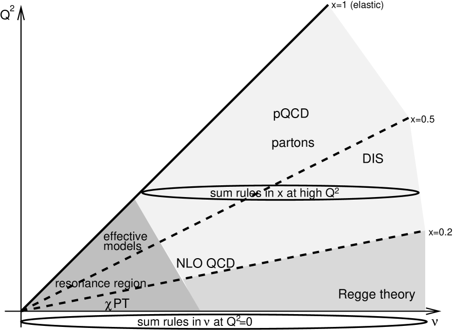
Figure 3: Kinematic regions and available descriptions of the strong interaction today

Some evidence for the “No-subtraction” hypothesis of the GDH Sum Rule to be true may be assumed as calculations within several perturbative models have verified the GDH Sum Rule. Moreover, explicitly also the high energy limit of the spin flip amplitude has been found to satisfy the “No-subtraction” hypothesis: Altarelli, Cabibbob and Maiani have verified that the Compton amplitude to fourth-order for the scattering of a photon off a charged lepton is finite in Weinberg’s model of weak and electro-magnetic interactions, and obeys the Gerasimov-Drell-Hearn sum rule [41]. Gerasimov and Moulin [42] have successfully tested the GDH sum rule in the pseudoscalar pion-nucleon model. Brodsky and Schmidt [43] have generalized the result of Ref. [41] to $2\to 2$ Standard Model and supersymmetric processes $\gamma a\to bc$ in the tree-graph approximation.

However, already in 1968, right after the discovery of the GDH Sum Rule, Abarbanel and Goldberger [30] considered a $J_{0}=1$ Regge fixed pole being a possible source for the failure of the No-Subtraction hypothesis. Such a $J_{0}=1$ fixed pole would allow the imaginary part of the spin-flip amplitude $f_{2}$ to vanish while $\lim\limits_{\nu\to\infty}\text{Re}\left[f_{2}(\nu)/\nu\right]\neq 0$. In the case of real Compton scattering this fixed pole also does not violate the Landau-Yang theorem: The Landau-Yang theorem forbids two photons to have a total angular momentum of $J_{0}=1$ [44, 45] in the center of mass system. This is to be related to the t-channel process with two external photon lines in the final state. For the s-channel Compton forward ($t=0$) amplitude $f_{2}$ both photons have the same helicity. Crossing relations (see Ref. [46]) then lead to a total helicity of 2 in the t-channel [15]. Hence, the total angular momentum has to be at least 2 and the Landau-Yang theorem does not apply. Also, the partial wave expansion includes only the values $J=2,3,\ldots$. This actually allows to consider this fixed pole at all.

Such a fixed pole is forbidden for purely hadronic processes but it cannot be ruled out a priori for electro-weak processes considered to low-order coupling only. Fairly recently, Bass [47] has revisited the possibility of such a fixed pole in view of possible gluonic and sea contributions. An observable effect of this would kick in only at very high energies. A connection of the fixed pole to the gluon topology is established. Bass conjectures a correction of up to 10 % to the GDH Sum Rule due to the fixed pole [48, 47].

However, such a fixed pole has never been observed explicitly so far and nature, of course, is not restricted in the electromagnetic coupling. Abarbanel, Low, Muzinich, Nussinov and Schwarz were the first to point out that bilinear unitarity in the $t$ channel also forbids a $J=1$ fixed pole [49]. For a general discussion of bilinear versus linear unitarity see for example [50, 51, 52, 53]. The principle idea is the following [54]: Consider the partial waves in the t-channel $a(t,J)$ of Compton scattering. With the fixed pole one would have

$$a(t,J)={\beta\over J-J_{0}}\quad\text{in the proximity of the pole }J_{0}=1\ .$$ (56)

Now we reconsider the optical theorem in terms of the $S$ and the $T$ matrix: $S=1+iT$. Unitarity gives $S^{\dagger}S=1$ or

$$\text{Im }T=\frac{1}{2}\;T^{\dagger}T\quad.$$ (57)

Here, the pole from Eq. (56) would enter quadratically on the left hand side and only linearly on the right hand side and we end up having a pole of second order on the left hand side and a pole of first order only on the right hand side. Due to this contradiction such a pole cannot contribute in nature with all orders of electromagnetic coupling  However, if we expand $T$ in orders of the electromagnetic coupling $T=T_{0}+T_{1}+T_{2}+\ldots$ where $T_{0}$ represents strong interactions only, one obtains separate equations for each order in electromagnetic coupling:

$$\text{Im }T_{0} = \frac{1}{2}\,T_{0}^{\dagger}T_{0}$$ (58)

$$\text{Im }T_{1} = \text{Re }T_{0}^{\dagger}T_{1}$$ (59)

$$\text{Im }T_{2} = \text{Re }T_{2}^{\dagger}T_{0}+\frac{1}{2}\,T_{1}^{\dagger}T_{1}$$ (60)

When we consider lowest order coupling Eq. (59) is relevant only. Here the pole from Eq. (56) appears to first order on both sides and it may be relevant.

In conclusion, the fixed $J_{0}=1$ Regge pole may exist as an artifact of the limitation of the calculation including only low-order coupling. In nature however it is forbidden by full (bilinear or quadratic) unitarity and a failure of the “No-subtraction” hypothesis also would violate fundamental ingredients of today’s field theories like all the other steps of the derivation of the GDH Sum Rule.

3 Polarized virtual photoabsorption

Fig. 4 depicts the kinematics and useful spin orientations of lepton beam and nucleon target. We have the following common invariant kinematic quantities: $Q^{2}=-q^{2}=(k-k^{\prime})^{2}=4EE^{\prime}\sin^{2}\theta/2$ is the four-momentum transfer to the nucleon or the virtuality of the photon with the scattering angle $\theta$ of the lepton. $\nu=q\cdot P/m=E-E^{\prime}$ is the lepton’s energy loss in the nucleon rest frame and the photon energy. Bjorken-$x$ is defined as usual as $x=Q^{2}/2m\nu$ which, in the parton model, is the fraction of the nucleon’s momentum carried by the struck quark. $y=q\cdot P/k\cdot P=\nu/E$ is the fraction of the lepton’s energy lost in the nucleon rest frame and $W^{2}=(P+q)^{2}=m^{2}+2m\nu-Q^{2}$ is the mass squared of the recoiling system against the scattered lepton and $\gamma=\sqrt{Q^{2}}/\nu$.

$$A_{\parallel}\ =\ \frac{\sigma^{\uparrow\downarrow}-\sigma^{\uparrow\uparrow}}{\sigma^{\uparrow\downarrow}+\sigma^{\uparrow\uparrow}}\ =\ \left(\hskip 36.98857pt\begin{minipage}{130.0pt} \begin{picture}(130.0,81.0)\begin{picture}(130.0,81.0)\immediate\ignorespaces\immediate\ignorespaces\immediate\ignorespaces\immediate\ignorespaces\immediate\ignorespaces{\immediate\immediate}\put(0.0,0.0){{\f@ynmf:fe\char 1\relax}}\ignorespaces\immediate\ignorespaces\immediate\ignorespaces\immediate\ignorespaces\immediate\ignorespaces\immediate\ignorespaces\immediate\ignorespaces\immediate\ignorespaces\immediate\ignorespaces\immediate\ignorespaces\immediate\ignorespaces\immediate\ignorespaces\immediate\ignorespaces\immediate\ignorespaces\immediate\ignorespaces\immediate\ignorespaces\immediate\ignorespaces\immediate\ignorespaces\immediate\ignorespaces\immediate\ignorespaces\immediate\ignorespaces \immediate\ignorespaces{\put(54.49849,46.13889){\makebox(0.0,0.0)[rt]{$q$}} \put(8.1916,-3.74132){\makebox(0.0,0.0)[rt]{$P,m,\Rightarrow$}} \put(8.1916,84.68372){\makebox(0.0,0.0)[rb]{$k,\Leftarrow$}} \put(130.8091,12.80347){\makebox(0.0,0.0)[lt]{$W$}} \put(121.77472,84.68254){\makebox(0.0,0.0)[lb]{$k^{\prime}$}} }\end{picture} \end{picture} \end{minipage}\ \ \ -\ \ \begin{minipage}{130.0pt} \begin{picture}(130.0,81.0)\begin{picture}(130.0,81.0)\immediate\ignorespaces\immediate\ignorespaces\immediate\ignorespaces\immediate\ignorespaces\immediate\ignorespaces{\immediate\immediate}\put(0.0,0.0){{\f@ynmf:fe\char 2\relax}}\ignorespaces\immediate\ignorespaces\immediate\ignorespaces\immediate\ignorespaces\immediate\ignorespaces\immediate\ignorespaces\immediate\ignorespaces\immediate\ignorespaces\immediate\ignorespaces\immediate\ignorespaces\immediate\ignorespaces\immediate\ignorespaces\immediate\ignorespaces\immediate\ignorespaces\immediate\ignorespaces\immediate\ignorespaces\immediate\ignorespaces\immediate\ignorespaces\immediate\ignorespaces \immediate\ignorespaces{\put(54.49849,46.13889){\makebox(0.0,0.0)[rt]{$q$}} \put(8.1916,-3.74132){\makebox(0.0,0.0)[rt]{$\Rightarrow$}} \put(8.1916,84.68372){\makebox(0.0,0.0)[rb]{$\Rightarrow$}} }\end{picture} \end{picture} \end{minipage}\right)/\sum$$

$$A_{\perp}\ =\ \frac{\sigma^{\downarrow\leftarrow}-\sigma^{\uparrow\leftarrow}}{\sigma^{\downarrow\leftarrow}+\sigma^{\uparrow\leftarrow}}\ =\ \left(\hskip 8.53581pt\begin{minipage}{130.0pt} \begin{picture}(130.0,81.0)\begin{picture}(130.0,81.0)\immediate\ignorespaces\immediate\ignorespaces\immediate\ignorespaces\immediate\ignorespaces\immediate\ignorespaces{\immediate\immediate}\put(0.0,0.0){{\f@ynmf:fe\char 3\relax}}\ignorespaces\immediate\ignorespaces\immediate\ignorespaces\immediate\ignorespaces\immediate\ignorespaces\immediate\ignorespaces\immediate\ignorespaces\immediate\ignorespaces\immediate\ignorespaces\immediate\ignorespaces\immediate\ignorespaces\immediate\ignorespaces\immediate\ignorespaces\immediate\ignorespaces\immediate\ignorespaces\immediate\ignorespaces\immediate\ignorespaces\immediate\ignorespaces\immediate\ignorespaces \immediate\ignorespaces{\put(54.49849,46.13889){\makebox(0.0,0.0)[rt]{$q$}} \put(8.1916,-3.74132){\makebox(0.0,0.0)[rt]{$\Uparrow$}} \put(8.1916,84.68372){\makebox(0.0,0.0)[rb]{$\Leftarrow$}} }\end{picture} \end{picture} \end{minipage}\ \ \ -\ \ \ \begin{minipage}{130.0pt} \begin{picture}(130.0,81.0)\begin{picture}(130.0,81.0)\immediate\ignorespaces\immediate\ignorespaces\immediate\ignorespaces\immediate\ignorespaces\immediate\ignorespaces{\immediate\immediate}\put(0.0,0.0){{\f@ynmf:fe\char 4\relax}}\ignorespaces\immediate\ignorespaces\immediate\ignorespaces\immediate\ignorespaces\immediate\ignorespaces\immediate\ignorespaces\immediate\ignorespaces\immediate\ignorespaces\immediate\ignorespaces\immediate\ignorespaces\immediate\ignorespaces\immediate\ignorespaces\immediate\ignorespaces\immediate\ignorespaces\immediate\ignorespaces\immediate\ignorespaces\immediate\ignorespaces\immediate\ignorespaces\immediate\ignorespaces \immediate\ignorespaces{\put(54.49849,46.13889){\makebox(0.0,0.0)[rt]{$q$}} \put(8.1916,-3.74132){\makebox(0.0,0.0)[rt]{$\Uparrow$}} \put(8.1916,84.68372){\makebox(0.0,0.0)[rb]{$\Rightarrow$}} }\end{picture} \end{picture} \end{minipage}\right)/\sum$$

Figure 4: Kinematics of inelastic charged lepton scattering: $k,k^{\prime}$ and $P$ are the four-momenta of the incoming and outgoing leptons and of the incoming nucleon, $m$ is the mass of the nucleon and $W$ is the invariant mass of the recoiling system $X$. For the energy range under consideration the exchanged particle can only be a photon. The exchanged photon has the four-momentum $q$. $\Rightarrow$ and $\Leftarrow$ denote spins in parallel and antiparallel to the lepton beam momentum in the nucleon rest frame. $\Uparrow$ indicates a nucleon spin perpendicular to the beam momentum and $\sum$ stands for the sum of cross sections of the two relative spin orientations. $A_{\parallel}$ and $A_{\perp}$ are the two experimentally accessible asymmetries. The parts below the dashed lines indicate the portion of the scattering process that correspond to polarized virtual photoabsorption.

Fig. 4 also provides the definitions for the experimental asymmetries $A_{\parallel},A_{\perp}$. We are, however, interested in the photoabsorption subprocess which is the lower part of the diagrams below the dashed lines and the asymmetries of this subprocess. The spin structure of a virtual photon is more involved than that of real photon due to the longitudinal polarization component. The polarized virtual photoabsorption cross section in the nucleon rest frame may be written as

$$\frac{d\sigma}{d\Omega\ dE^{\prime}}=\Gamma_{V}\left[\sigma_{T}+\epsilon\sigma_{L}-P_{e}P_{x}\sqrt{2\epsilon(1-\epsilon)}\ \sigma_{LT}-P_{e}P_{z}\sqrt{1-\epsilon^{2}}\ \sigma_{TT}\right]$$ (61)

with the photon polarization $\epsilon$ relative to the lepton polarization $P_{e}$, the virtual photon flux factor $\Gamma_{V}$ and the equivalent photon energy $K$

$$\epsilon=\frac{1}{1+2(1+\nu^{2}/Q^{2})\tan^{2}\theta/2}\ ,\quad\Gamma_{V}=\frac{\alpha}{2\pi^{2}}\ \frac{E^{\prime}}{E}\ \frac{K}{Q^{2}}\ \frac{1}{1-\epsilon}\ ,\quad K=\nu(1-x)=\frac{W^{2}-m^{2}}{2m}\ .$$ (62)

$P_{z}$ and $P_{x}$ denote the components of the target polarization in the direction of the virtual photon momentum ${\vec{q}}$ and perpendicular to that direction in the scattering plane of the electron. In addition to the transverse cross sections $\sigma_{T}$ and $\sigma_{TT}$, the virtuality of the photon gives rise to the longitudinal $\sigma_{L}$ and the longitudinal-transverse $\sigma_{LT}$ cross sections.

With these definitions we have the photoabsorption asymmetries $A_{1}$ and $A_{2}$:

$$A_{1}=\frac{\sigma_{1/2}-\sigma_{3/2}}{\sigma_{1/2}+\sigma_{3/2}}=\frac{\sigma_{TT}}{\sigma_{T}}\ ,\quad A_{2}=\frac{2\,\sigma_{TL}}{\sigma_{T}}$$ (63)

For transverse polarization of the photon the subscripts $3/2$ and $1/2$ denote the total helicity of the photon-nucleon system in the nucleon rest frame with respect to the center of mass momentum. $\sigma_{TL}$ is the longitudinal-transverse virtual photoabsorption cross section. The experimentally directly observable asymmetries $A_{\parallel},A_{\perp}$ of the lepton scattering process are related to the asymmetries $A_{1},A_{2}$ in the photoabsorption process by kinematic factors:

$$A_{\parallel}=D(A_{1}+\eta A_{2})\ ,\quad A_{\perp}=d(A_{2}-\xi A_{1}),$$ (64)

The kinematic factors read

$$D=\frac{1-\epsilon E^{\prime}/E}{1+\epsilon R}\,\quad d=\frac{\sqrt{1-y-\gamma^{2}y^{2}/4}}{1-y/2}\,D\ ,\quad\eta=\frac{\gamma\,(1-y-\gamma^{2}y^{2}/4)}{(1-y/2)(1+\gamma^{2}y/2)}\ ,\quad\xi=\frac{\gamma(1-y/2)}{1+\gamma^{2}y/2}~{}\ .$$ (65)

where $R$ is the ratio of longitudinal to transverse virtual photoabsorption cross sections.

3.1 Deep inelastic scattering

The process in Fig. 4 is called deep inelastic scattering if $Q^{2}>>m^{2},W^{2}>>m^{2}$. One can then neglect the mass of the scattered lepton. In lowest order perturbation theory the cross section for the scattering factorizes into a leptonic $L^{\mu\nu}$ and a hadronic tensor $W^{\mu\nu}$:

$$\frac{d^{2}\sigma}{dxdy}=\frac{2\pi y\alpha^{2}}{Q^{4}}L^{\mu\nu}W_{\mu\nu}$$ (66)

The lepton tensor associated with the exchange of a photon reads

$$L_{\mu\nu}=2\left(k_{m}uk^{\prime}_{\nu}+k^{\prime}_{\mu}k_{\nu}-k\cdot k^{\prime}g_{\mu\nu}-i\lambda\epsilon_{\mu\nu\alpha\beta}k^{\alpha}k^{\prime\beta}\right)$$ (67)

with the helicity $\lambda=\pm 1$ of the incoming lepton. The hadronic tensor describes the interaction of the virtual photon with the target nucleon and this is where the internal structure of the nucleon is manifest. Since this structure cannot (yet) be obtained directly by application of QCD for all kinematic regions this hadron tensor is parameterized by eight structure functions [56]. For deep inelastic scattering where the momentum transfer is small compared to the mass of the $Z^{0}$ boson, contributions from weak interactions can be neglected and we have to consider only four independent structure functions. $W^{\mu\nu}$ can be split into a symmetric and an anti-symmetric part:

$$W^{\mu\nu}=W^{\{\mu\nu\}}+W^{[\mu\nu]},$$ (68)

with

$$W^{\{\mu\nu\}} = \left(-g^{\mu\nu}+{q^{\mu}q^{\nu}\over q^{2}}\right)F_{1}+\left[\left(P^{\mu}-{\nu\over q^{2}}q^{\mu}\right)\left(P^{\nu}-{\nu\over q^{2}}q^{\nu}\right)\right]{F_{2}\over\nu},$$ (69)

$$W^{[\mu\nu]} = -i\varepsilon^{\mu\nu\lambda\sigma}q_{\lambda}\left({s_{\sigma}\over\nu}\left(g_{1}+g_{2}\right)-{q\cdot s\ P_{\sigma}\over\nu^{2}}g_{2}\right),$$ (70)

where $s$ is the nucleon covariant spin vector $(s^{2}=-m^{2})$, $P\cdot s=0$ and $\varepsilon^{\mu\nu\lambda\sigma}$ is the totally antisymmetric Levi-Civita tensor. $g_{1,2}$ and $F_{1,2}$ are scalar dimensionless functions. These structure functions are related to others in common use by:

$$W_{1}=F_{1},\quad W_{2}={m^{2}\over\nu}F_{2},\quad G_{1}={m\over\nu}\,g_{1},\quad G_{2}={m^{2}\over\nu^{2}}\,g_{2}.$$ (71)

For the absorption of transversely polarized virtual photons by longitudinally polarized nucleons with total spin $3/2\ \mbox{and}\ 1/2$ the result of this tensor product reads:

$$\sigma_{3/2} = \frac{8\pi^{2}\alpha}{2m\nu-Q^{2}}\left(F_{1}(x,Q^{2})-g_{1}(x,Q^{2})+\frac{Q^{2}}{\nu^{2}}g_{2}(x,Q^{2})\right)$$ (72)

$$\sigma_{1/2} = \frac{8\pi^{2}\alpha}{2m\nu-Q^{2}}\left(F_{1}(x,Q^{2})+g_{1}(x,Q^{2})-\frac{Q^{2}}{\nu^{2}}g_{2}(x,Q^{2})\right)$$ (73)

We can now express the virtual photoabsorption asymmetry $A_{1}$ in terms of these structure functions:

$$A_{1}=\frac{g_{1}-\gamma^{2}\,g_{2}}{F_{1}}\simeq\frac{g_{1}}{F_{1}}$$ (74)

In the quark-parton model the quark densities depend only on the momentum fraction $x$ carried by the quark. In the infinite momentum frame, due to angular momentum conservation, a virtual photon with helicity $+1$ or $-1$ can only be absorbed by a quark with a spin projection of $-\frac{1}{2}$ or $+\frac{1}{2}$, respectively. $g_{1}(x)$ is then given by

$$g_{1}(x)=\frac{1}{2}\sum_{i=1}^{n_{f}}e_{i}^{2}\Delta q_{i}(x),$$ (75)

where

$$\Delta q_{i}(x)=q_{i}^{+}(x)-q_{i}^{-}(x)+\bar{q}_{i}^{~{}+}(x)-\bar{q}_{i}^{~{}-}(x),$$ (76)

$q_{i}^{+}(\bar{q}_{i}^{~{}+})$ and $q_{i}^{-}(\bar{q}_{i}^{~{}-})$ are the distribution functions of quarks (antiquarks) with spin parallel and antiparallel to the nucleon spin, respectively, $e_{i}$ is the electric charge of the quarks of flavor $i$ and $n_{f}$ is the number of quark flavors involved.

3.1.1 Bjorken sum rule

The Bjorken sum rule [57] and the Ellis-Jaffe sum rule [6] are the counterpieces of the GDH sum rule. While the GDH Sum Rule is a statement at $Q^{2}=0$ the Bjorken and the Ellis-Jaffe sum rule are predictions at infinite $Q^{2}$.

J. D. Bjorken derived his sum rule in 1966 which is the very same year that the GDH Sum Rule was proposed. Initially, Bjorken himself disqualified the sum rule in his own publication:

Something may be salvaged from this worthless equation …

However, he reconsidered his sum rule in 1970 “in light of the present experimental and theoretical situation”. He was referring to an article [58] on inelastic electron scattering results from Slac that showed that “for high excitations the cross section shows only a weak momentum-transfer dependence”. Today, this phenomenon is called Bjorken scaling and is discussed in about all modern text books on particle physics.

The representation of the Bjorken sum rule in the original article [57] (Eq. (6.16) and (6.17) therein) shows the similarity of it to the GDH Sum Rule for real photoabsorption:

$$\lim_{q^{2}\to-\infty}\lim_{E\to\infty}\int_{0}^{\infty}\frac{d\nu^{\prime}}{\nu^{\prime}}\left[\frac{d\sigma_{3/2}-d\sigma_{1/2}}{dq^{2}d\nu^{\prime}}\right]=-\frac{8\pi\alpha^{2}}{q^{4}E}Z_{N}\quad\text{with}\quad Z_{p}-Z_{n}=\frac{1}{3}\left(\frac{g_{A}}{g_{V}}\right)$$ (77)

${g_{A}}/{g_{V}}$ is the ratio of the phenomenological weak $\beta$-decay coupling constants. Bjorken in his article only briefly states that the values of the constants $Z_{N}$ are unknown but that $SU(6)$ symmetry would lead to $Z_{p}=5/9$ and $Z_{n}=0$ (see also Sec. 3.1.2). Like in the derivation of the GDH Sum Rule by means of the equal-times current algebra in Sec. 2.2.1 the starting point for the derivation of the Bjorken sum rule also is the vanishing of the quark-model equal-time commutator for the space components (see Eq. (42)). Bjorken’s proof also relies on a “No-subtraction” hypothesis. Again like the GDH Sum Rule, the Bjorken sum rule also connects static properties of the nucleon with its dynamic response. In today’s nomenclature the Bjorken sum rule is usually represented like

$$\lim_{Q^{2}\to\infty}\left[\,\Gamma_{1}^{p}(Q^{2})-\Gamma_{2}^{n}(Q^{2})\,\right]=\frac{1}{6}\left|\frac{g_{A}}{g_{V}}\right|$$ (78)

with the definition for the first moment of the proton or the neutron structure functions $g_{1}$

$$\Gamma_{1}(Q^{2})=\int\limits_{0}^{1}g_{1}(x,Q^{2})\,dx\quad.$$ (79)

Through the neutron decay parameter of $n\to pe^{-}\bar{\nu}_{e}$ this ratio is known very accurately [36]: $\lambda\equiv g_{A}/g_{V}=-1.2695\pm 0.0029$.

Hence, the right hand side of the Bjorken sum rule Eq. (78) is known with a relative precision of about $2.3\cdot 10^{-3}$. In comparison to the dynamic observables this is an impressive precision already. On the other hand, the ratio of the magnetic moment of the proton $\mu_{p}$ to the nuclear magneton $\mu_{N}$ that leads to the anomalous magnetic moment in the GDH Sum Rule has been measured to an even higher precision [59]: $\mu_{p}/\mu_{N}=2.792847351\pm 0.000000028$ which is a relative precision of $10^{-8}$. For the time being there seems to be no chance to come even close to these accuracies with the verification of these sum rules as the measurements of the dynamic observables and cross sections have a systematic error of the order of several percent originating for example from the determination of the polarizations of target and beam.

However, the dominant limitation of a verification of the Bjorken sum rule stems from the $Q^{2}$ evolution which is necessary since $Q^{2}\to\infty$ is not reachable experimentally. At finite values of $Q^{2}$ radiative QCD corrections are important. Beyond leading order the corrections also depend on the renormalization scheme and the number of flavors taken into account. At $Q^{2}=10~{}\text{GeV}^{2}$ for example the correction is about a factor of $7$. Also the experimental data obtained at fixed beam momentum need to be evolved to a common $Q^{2}$ in order to perform the integration in $x$ of Eq. (79) at fixed $Q^{2}$. Both these $Q^{2}$ evolutions of the theoretical Bjorken sum rule prediction and the experimental data impair the fundamental character the sum rule originally has at $Q^{2}=\infty$. Hence an experimental verification of the Bjorken sum rule cannot claim to be a test of its fundamental principles like it is the case with the GDH Sum Rule but is rather a check of our understanding of QCD, higher order corrections and of scaling violation.

Several experiments have performed verifications of the $Q^{2}$-evolved Bjorken sum rule. Most recently the Hermes-Collaboration at Desy reported [60] an agreement within the experimental error of about 12 % at a $Q^{2}=2.5~{}\text{GeV}^{2}$. The experimental error does not include an estimate of the error of extrapolation to unmeasured regions in Bjorken-x. The Spin Muon Collaboration (SMC) at Cern has combined their own data [61] with the data from their precursor experiment EMC [8] also at Cern and the E80/E130 [62, 63, 7] and E142/E143  [64, 65] experiments at Slac. They find agreement with the Bjorken sum rule at $Q^{2}=10~{}\text{GeV}^{2}$ within 19 % experimental uncertainty and at $Q^{2}=5~{}\text{GeV}^{2}$ within 11 % experimental error including estimates of the uncertainties arising from the Bjorken-x extrapolation.

All in all, there is no hint that the Bjorken sum rule may be wrong and it seems that the QCD $Q^{2}$-evolution is well under control to the level of about 10 %.

3.1.2 Ellis-Jaffe sum rules

J. R. Ellis and R. L. Jaffe [6] in 1974 have derived similar sum rules like the Bjorken sum rule. The Ellis-Jaffe sum rules are statements for the proton and the neutron individually. They are obtained by assuming exact SU(3) flavor symmetry and a sea contribution from strange quarks without a resulting polarization:

$$\int\limits_{0}^{1}g_{1}^{p}(x)\,dx=\frac{9F-D}{18}\qquad\int\limits_{0}^{1}g_{1}^{n}(x)\,dx=\frac{6F-4D}{18}$$ (80)

The constants $F$ and $D$ are SU(3) invariant matrix elements of the axial vector current where for the neutron beta decay $F+D=g_{A}/g_{V}$ [66].

Several experiments have reported a violation of the Ellis-Jaffe sum rules. Most prominently, already in 1989 the European Muon Collaboration (EMC) claimed a disagreement with the Ellis-Jaffe sum rule for the Proton [8]. In the naïve parton model the results lead to the conclusion that the total quark spin constitutes only a small fraction of the spin of the proton. This finding lead to the so-called “spin crisis” which sparked a whole series of spin physics experiments. Today, the combined data from the Slac experiments E80/E130 and E142/E143 and from EMC and SMC at Cern show a discrepancy of about 2 standard deviations for the proton and about three standard deviations for the deuteron at an evolved $Q^{2}=10~{}\text{GeV}^{2}$.

The origin of this discrepancy may be a polarization of the strange quark content. The Hermes experiment at Desy has performed the first direct experimental extraction of the separate helicity densities of the light quark sea [67]. For strange sea quarks in a leading order QCD analysis the results do not fully explain the discrepancies found for the Ellis-Jaffe sum rules as the strange quark polarization appears rather small.

On the other hand a sizable gluon polarization could also change the interpretation of the structure functions at finite photon virtualities. In this case the polarized structure function $g_{1}$ does not only represent the polarization of the quarks like at $Q^{2}=\infty$ where we have Eq. (75). Instead, the quark and the gluon spin content both are important for $g_{1}$ at intermediate virtualities. It is one of the main goals of the Compass experiment at Cern and the Rhic spin program at BNL to determine the gluon polarization [68, 69].

3.2 Extension of the GDH Sum to finite photon virtuality

There are several ways to generalize the integral on left hand side of the GDH Sum Rule i.e. the integral over all energies. For an overview see for example Ref. [70]. Amongst these choices experimentalists sometimes favor a version which is a straight forward generalization of the GDH Sum Rule in terms of the polarized photoabsorption cross section:

$$I_{\text{GDH}}(Q^{2}) = {\boldsymbol{-}}\int\limits_{0}^{\infty}d\nu\,\frac{\sigma_{3/2}(\nu,Q^{2})-\sigma_{1/2}(\nu,Q^{2})}{\nu}=\frac{8\pi^{2}\alpha}{m^{2}}\int\limits_{0}^{\infty}d\nu\frac{G_{1}(\nu,Q^{2})-\frac{Q^{2}}{m\nu}\,G_{2}(\nu,Q^{2})}{\sqrt{\nu^{2}+Q^{2}}}$$ (81)

$$= \frac{16\pi^{2}\alpha}{Q^{2}}\int\limits_{0}^{1}dx\,\frac{g_{1}(x,Q^{2})-\xi\,g_{2}(x,Q^{2})}{\sqrt{1+\xi}}\quad\text{with }\xi=\frac{4m^{2}x^{2}}{Q^{2}}$$

This definition is close to the measured observables. On the other hand, theorists often prefer the following integral related to the first moment $\Gamma_{1}$ because it is related to only a single structure function namely $g_{1}$ (see Eq. (79)):

$$I_{1}(Q^{2})=\frac{2m^{2}}{Q^{2}}\Gamma_{1}(Q^{2})=\frac{2m^{2}}{Q^{2}}\int\limits_{0}^{1}dx\ g_{1}(x,Q^{2})=\int\limits_{0}^{\infty}\frac{d\nu}{\nu}\ G_{1}(\nu,Q^{2})$$ (82)

In the real photon limit we obtain the limits for both generalized integrals from the GDH Sum Rule

$$I_{\text{GDH}}(0)=-\frac{2\pi^{2}\alpha}{m^{2}}\kappa^{2}\quad\text{and}\quad I_{1}(0)=\frac{m^{2}}{8\pi^{2}\alpha}I_{\text{GDH}}(0)=-{1\over 4}\kappa^{2}$$ (83)

while in the scaling limit both generalized integrals coincide

$$Q^{2}\to\infty:~{}I_{\text{GDH}}(Q^{2})=I_{1}(Q^{2})\quad\text{with the Bjorken sum rule}\ \left[I_{1}^{p}(Q^{2})-I_{1}^{n}(Q^{2})\right]={m^{2}\over 3Q^{2}}\,{g_{A}\over g_{V}}\ .$$ (84)

Recently, Ji and Osborne [71, 72] have developed a unified formalism to describe the generalized GDH integral $I_{1}$ with respect to the doubly-virtual Compton forward scattering (VVCS) process. One considers the forward scattering of a virtual photon with space-like four-momentum $q^{2}=q_{0}^{2}-\vec{q}\,^{2}=-Q^{2}<0$. The VVCS amplitude for forward scattering of virtual photons generalizes Eq. (5) by introducing an additional longitudinal polarization vector $\vec{\hat{q}}$,

$$T(\theta=0,\nu,\,Q^{2})=f_{1}\ \vec{\epsilon_{2}}^{\ast}\cdot\vec{\epsilon_{1}}+f_{2}\ i\vec{\sigma}\cdot(\vec{\epsilon_{2}}^{\ast}\times\vec{\epsilon_{1}})+f_{3}\ +f_{4}\ i\,(\vec{\epsilon_{2}}^{\ast}-\vec{\epsilon_{1}})\cdot(\vec{\sigma}\times\vec{\hat{q}}\,)$$ (85)

$f_{1,2}(\nu,Q^{2})$ are now functions of $\nu$ and $Q^{2}$ and coincide with those of Eq. (5) at $Q^{2}=0$ while the functions $f_{3,4}(\nu,Q^{2})$ are due to the longitudinal polarization components of the virtual photon. To connect the VVCS amplitudes with the nucleon structure functions one writes Eq. (85) in a covariant form and separates the spin independent $T^{\{\mu\nu\}}$ and spin dependent amplitudes $T^{[\mu\nu]}$ with $T^{\mu\nu}=T^{\{\mu\nu\}}+T^{[\mu\nu]}$. We are interested in the spin dependent part which reads

$$T^{[\mu\nu]}(\nu,Q^{2},\theta=0)\ =\ \frac{i}{2}\,\epsilon_{2_{\mu}}^{\ast}\epsilon_{1_{\nu}}\,\varepsilon^{\mu\nu\alpha\beta}\,\left\{q_{\alpha}s_{\beta}\,S_{1}(\nu,Q^{2})+\frac{1}{m^{2}}\,q_{\alpha}(P\cdot q\ s_{\beta}-s\cdot q\ P_{\beta})\,S_{2}(\nu,Q^{2})\right\}\ .$$ (86)

$\varepsilon_{\mu\nu\alpha\beta}$, $P$ and $s$ are defined as before with Eq. (69). We are mainly interested in the forward scattering amplitude $S_{1}(\nu,Q^{2})$ which is connected to $f_{2}(\nu,Q^{2})$ in the real photon case (see Eqs. (5) and (85)). From general principles (causality and unitarity) as well as an assumption about the large-$\nu$ behavior of $S_{1}(\nu,Q^{2})$ – similar to the “No-subtraction” hypothesis discussed in the context of $f_{2}$ – one can now write down a dispersion relation

$$S_{1}(\nu,Q^{2})=\frac{16\pi\alpha}{m^{2}}\,\int\limits_{0}^{\infty}\frac{\nu^{\prime}d\nu^{\prime}\;G_{1}(\nu^{\prime},Q^{2})}{\nu^{\prime 2}-\nu^{2}}$$ (87)

where we have used the optical theorem $\text{Im }S_{1}(\nu,Q^{2})=2\pi G_{1}(\nu,Q^{2})$.

While $G_{1}(\nu^{\prime},Q^{2})$ is difficult to calculate it can be measured experimentally. On the other hand, $S_{1}(\nu^{\prime},Q^{2})$ is hard to measure experimentally but it can be calculated theoretically in terms of the VVCS process. Again like with the derivation of the GDH Sum Rule one takes the limit $\nu\to 0$:

$$\bar{S}_{1}(0,Q^{2})=\frac{16\pi\alpha}{m^{2}}\int\limits_{\nu_{0}}^{\infty}\frac{d\nu^{\prime}}{\nu^{\prime}}\ \bar{G}_{1}(\nu^{\prime},Q^{2})=\frac{16\pi\alpha}{m^{2}}\,\bar{I}_{1}(Q^{2})$$ (88)

were $\bar{S}_{1,2}=S_{1,2}-S^{\text{el}}_{1,2}$ are the amplitudes without the elastic intermediate state and $\bar{G}_{1},\ \bar{I}_{1}$ the like, $\nu_{0}$ is the inelastic threshold.

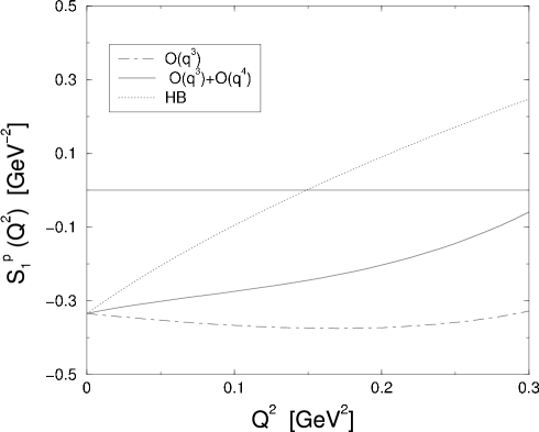
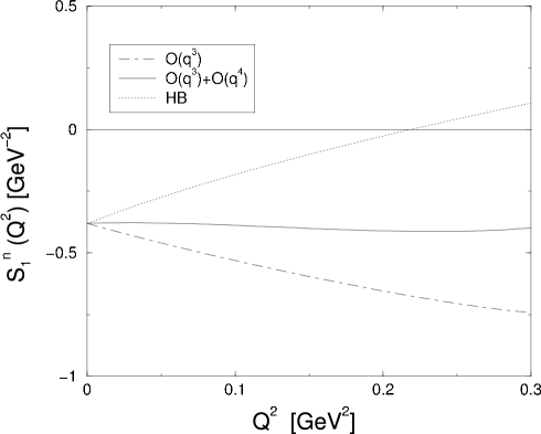
Figure 5: Chiral loop contribution to the structure function $\bar{S}_{1}(0,Q^{2})$ with the elastic contribution subtracted. The solid (dot-dashed) line gives the result of the calculation [73] to order $q^{4}$ ($q^{3})$ in comparison to the heavy baryon result of [74] (dotted line). Left (right) panel: Proton (neutron). Source: Ref. [73]

At $Q^{2}>1$ GeV² QCD operator product expansions should yield the value of $\bar{S}_{1}$ while at $Q^{2}<0.1$ GeV² chiral perturbation theory calculations are used. However, it turns out that the chiral calculations have not yet converged. A comparison of calculations in the heavy baryon approach by Ji, Kao and Osborne [74] with calculations done by Bernard, Hemmert and Meissner [73] shows that both approaches do not agree and moreover, that the chiral expansion has not yet converged (see Fig. 5). The level of uncertainty already at $Q^{2}=0.1$ GeV² for $\bar{S}_{1}(Q^{2})$ is of the order of 50 % while the value of $\bar{S}_{1}$ at $Q^{2}=0$ is already taken from the GDH Sum Rule prediction.

Figure 6: The generalized GDH integral $I_{1}(Q^{2})$ as defined in the text. Shown are data from the Hermes experiment at Desy [75] (filled triangles), from the E143 experiment at Slac [76] (open squares), from the EG1a experiment using the Clas detector at JLab [77] (filled circles) and preliminary data from the EG1b experiment [78] (open circles).

Despite, there is no stringent rule to these integrals established at finite $Q^{2}$, one can study the transition from hadronic degrees of freedom to partonic structure. Fig. 6 shows this transition in terms of the generalized GDH integral $I_{1}(Q^{2})$. At large $Q^{2}$ with $Q^{2}>2$ GeV² one observes a $1/Q^{2}$ behavior which is due to Bjorken scaling. Around $Q^{2}=1$ GeV² a dramatic change sets on and at about $Q^{2}=0.25$ GeV² the sign of the generalized integral changes toward the negative value of the GDH sum rule prediction. At even lower momentum transfer the generalized integral shows a very steep slope.

However, even at the lowest momentum transfer accessible nowadays of $Q^{2}\simeq 0.05$ GeV² one is still about a factor of 2 away from the GDH Sum Rule prediction. Taken together with the observation of the steep slope in Fig. 6 it appears hopeless to estimate the GDH integral at the real photon point with a reasonable precision and it appears imperative to measure the GDH sum rule at the real photon point with exactly $Q^{2}=0$. This measurement at the real photon point is what we will focus on in the following.

4 The GDH-Experiment at ELSA and MAMI

The magnetic moment of the proton in nuclear magnetons ${}_{p}/_{N}$, is the ratio of the spin axis precession frequency of a proton in a magnetic field to the frequency of the proton’s orbital motion in the same field, called the cyclotron frequency. In this ratio the typically dominant experimental error, the magnetic field strength, cancels mostly. Frequencies are amongst the most precisely measurable quantities in physics. Consequently, the proton anomalous magnetic moment is known today with a relative precision of $10^{-8}$. Also the mass of the proton is known with that precision. That is why the GDH Sum Rule is a very stringent prediction.

To verify the GDH Sum Rule the integral in photon energy over the polarized total cross sections – i.e. the left hand side of Eq. (1) – has to be determined experimentally.

4.1 Experimental concept

The dynamic observables on the left hand side of the Gerasimov-Drell-Hearn sum rule (Eq. (1)) need to be measured in a large energy range to ensure that contributions from unmeasured energy regions only represent minor uncertainties. The GDH-Collaboration has chosen to perform the measurement of the integrand of the sum rule at two accelerators: Elsa in Bonn and Mami in Mainz, Germany. This covers the energy range from pion threshold at 140 MeV up to 3 GeV. The measurements at Mami are dedicated to the lower energy part up to 800 MeV while, with an overlap, the measurements at Elsa address photon energies of 600 MeV through 3 GeV. In total this allows to cover the whole resonance region and to reach the onset of the Regge regime. The resonances allow to study the hadronic spin structure in detail while the Regge regime ultimately provides a description of the part of the integration up to infinite energies that is not accessible experimentally.

The photons needed to study the photoabsorption cross section are produced by bremsstrahlung of the primary electrons from the accelerators (Sec. 4.4.1). At both accelerator sites a tagging spectrometer is used to identify the photon energy and to determine the photon flux.

The relative helicity states of photon and proton of $3/2$ (parallel) and $1/2$ (antiparallel) are obtained by a fixed polarized solid state target (Sec. 4.5) and by means of a polarized electron beam (Sec. 4.2). The polarization of the electrons is (partially) transfered to the photons in the bremsstrahlung process (see Sec. 4.4.1). The degree of polarization of the electron beam is obtained by Møller polarimetry (Sec. 4.3).

Finally, the cross sections for the different spin configurations of the GDH Sum Rule have to be determined. As discussed in Secs. 2.1.3 and 2.4.1 it is sufficient to focus on photoabsorption which is experimentally more convenient than measuring the total cross section including elastic contributions. The lowest energy with a non-vanishing photoabsorption cross section is the pion threshold at 140 MeV photon energy in the nucleon rest frame. The photoabsorption cross sections are determined by hadronic final states with two detectors: The GDH-Detector at Elsa and Daphne at Mami together with additional components in forward direction (see Sec. 4.6). Since the difference $\sigma_{3/2}-\sigma_{1/2}$ is only about a 0.1 % effect compared to unpolarized total event rates – given the experimental conditions like effective polarization and background from unpolarized material – these detectors need to be capable of determining the absolute cross sections very reliably.

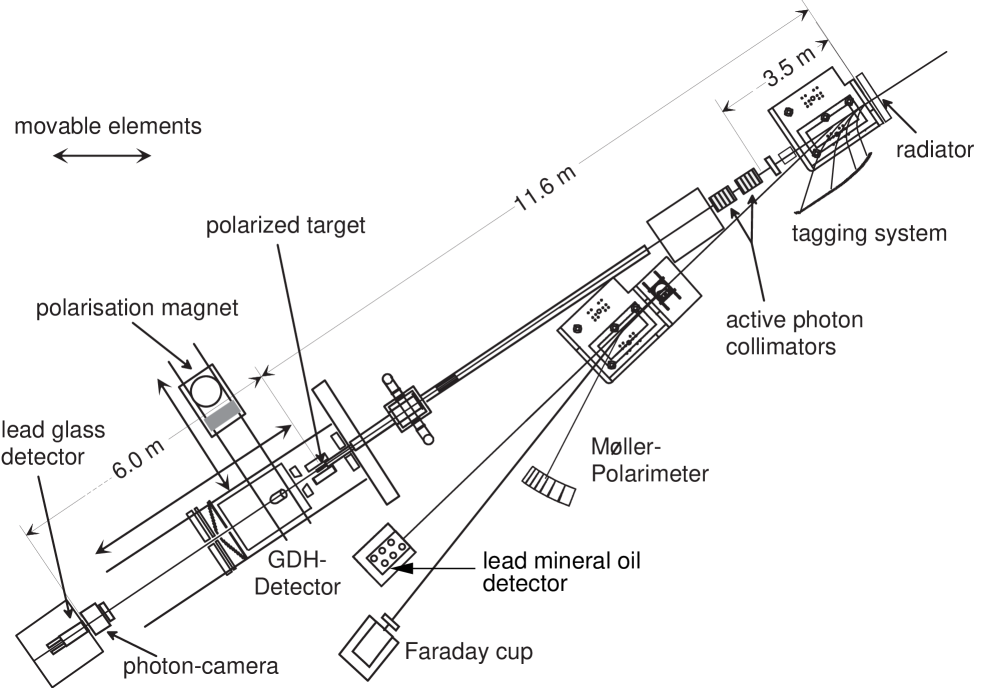
Figure 7: Experimental setup of the GDH-Experiment at Elsa

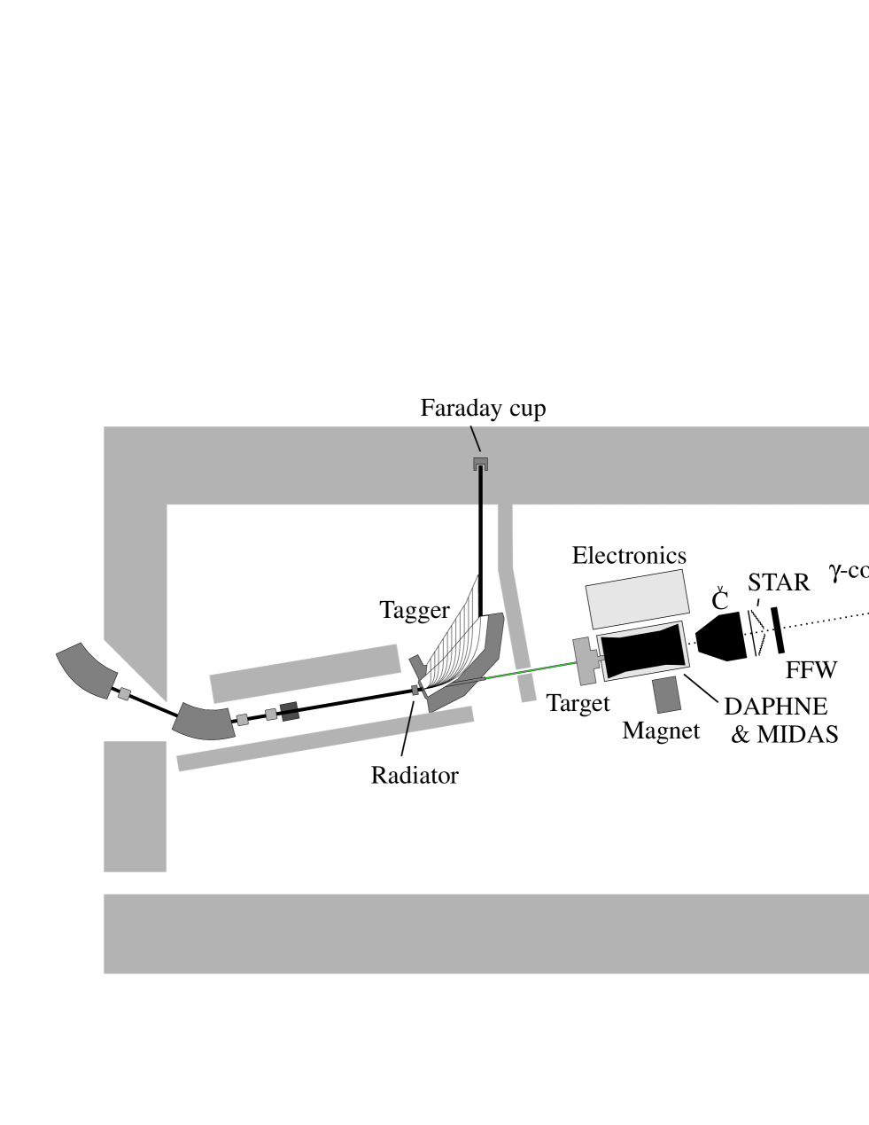
Figure 8: Experimental setup of the GDH-Experiment at Mami

Fig. 7 shows the experimental setup of the GDH-Experiment at Elsa. The setup at Mami is shown in Fig 8. The setup at Mami is very similar to the one at Elsa with the exception of the Møller polarimeter and the subsequent devices that are not present at Mami. At Mami M ller polarimetry was incorporated into the tagging system (see Sec. 4.3.2). In both cases the electron beam first impinges on the bremsstrahlung radiator. At Elsa the primary electrons then reach the Møller polarimeter. The photon beam is collimated and guided through a vacuum system to the polarized target. The polarized target is hermetically surrounded by a detector (the GDH-Detector or Daphne) which determines the total cross section. At Elsa both the lead glass detector and the lead mineral oil detector serve as vetos for background processes. The beam dumps for photon and electron beams contain beam diagnostic devices.

4.2 Electron beam polarization

4.2.1 Polarized electrons at MAMI

The electron accelerator Mami B is operated by the institute for nuclear physics of Mainz university. It serves experiments with electrons (virtual photons) and real photons. Polarized electrons can be accelerated up to a maximum energy of 855 MeV. A sketch of Mami B including the experimental area of the GDH-Experiment is represented in Fig. 9. The pulse frequency of the accelerator is 2450 MHz, which corresponds to a bunch distance of about 400 ps.

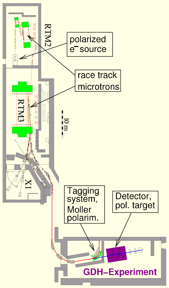
Figure 9: The GDH-Experiment at Mami.

Polarized electrons are produced by photoelectric effect at a gallium arsenide crystal [79]. A “strained layer” of a GaAs_0.95P_0.5 photocathode is exposed to circularly polarized laser light. The obtained electron current is over 10 $\upmu$A with a polarization degree of approximately 75 %. In the magnetic dipole fields of the accelerator the spin of the electrons rotates faster than the angular frequency because of the g-factor anomaly. The beam polarization orientation at the radiator for bremsstrahlung depends on the beam energy. The injection system of the polarized electron source is too compact to incorporate a spin rotating system to compensate for this. Instead, the longitudinal orientation of the polarization at the bremsstrahlung radiator is achieved by fine tuning of the exact energy gain of the microtron and the input energy. Two electron beam energies 855 MeV and 525 MeV were used for the GDH-Experiment.

For the GDH-Experiment the spin orientations parallel and antiparallel to the target spin are used. To obtain these two orientations and to minimize systematic effects the helicity of the laser light at the polarized source is changed every two seconds.

4.2.2 Polarized electrons at ELSA

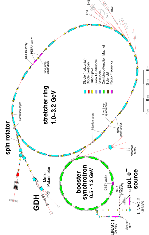
Figure 10: The GDH-Experiment at Elsa. Shown in bold face are the components crucial for the electron beam polarization and the GDH experiment.

The electron accelerator Elsa is operated by the physics institute of the university of Bonn. Fig. 10 shows the general layout of the electron accelerator Elsa which consists of 2 alternative Linacs with corresponding electron sources, a synchrotron and the stretcher ring. Electrons coming from one of the three available electron sources (2 polarized and 1 unpolarized) are pre-accelerated in Linac 1 (120 keV polarized source or thermionic gun) or Linac 2 (50 keV polarized source) [80], respectively. This quasi continuous electron beam is converted by a prebuncher into a 50 Hz pulsed beam before it is injected into the synchrotron. In the synchrotron the electrons are accelerated up to a maximum energy of 1.6 GeV. For the GDH-Experiment 1.2 GeV were used. The electrons are then injected into the stretcher ring. Up to 28 shots of the synchroton, which corresponds to an injection time of 480 ms guarantee a homogeneous filling of the stretcher ring. After injection, the electrons are further accelerated (up to 3.5 GeV). The accelerating cavities are operated at 500 MHz which corresponds to a bunch time structure with a period of 2 ns. The electron bunches have a width of 50 ps. The electrons in the stretcher ring can either be stored inside the ring for experiments with synchrotron light or they can be extracted to external experiments. For the extraction of the electrons from the storage ring the spatial distribution of the electrons is increased by magnetic quadrupoles. Electrons at the edge of the beam are deflected into the external beam line by 2 septum magnets.

Polarized electrons at Elsa are available up to 3.2 GeV [81, 82] with an intensity of up to 2 nA at the experiment and a duty-cycle of up to 95 %. A beam polarization of up to $73~{}\%$ parallel to the magnetic field in the dipoles of the stretcher ring has been achieved. During acceleration in a ring accelerator with non-deterministic particle tracks only the vertical polarization component is conserved. Since the experiment requires longitudinally polarized electrons, the electron spin has to be rotated in the external beam line. By means of a super conducting solenoid magnet the vertical spin is rotated around the longitudinal axis into the horizontal plane. In the adjacent dipole magnets the spin is rotated around the vertical axis due to Thomas-precession into the longitudinal direction.

This process, however, can be incomplete. At 2.46 GeV, the maximum field strength of the solenoid magnet is reached and a vertical spin component remains. This effect together with the occurrence of depolarizing resonances due to imperfections of the magnetic field of the accelerator was the motivation to build a Møller polarimeter that allows to study all three spatial spin components as fast as possible at Elsa (Sec. 4.3.1).

The electron beam helicity is randomly reversed at the source every few seconds to give access to the different relative spin orientations.

4.3 Møller polarimetry

Mott polarimeters are employed to determine the degree of polarization at low energies. At Elsa and at Mami, Mott polarimeters are suited to monitor the performance of the electron source before the acceleration process can have an impact on the polarization.

Compton and Møller polarimeters are used to measure the polarization of high energy electron beams. While Compton polarimeters are widely employed to measure the electron polarization of high intensity beams for example in storage rings or linear accelerators, Møller polarimeters are the natural choice for low intensity electron beams due to the large cross section.

4.3.1 Møller polarimetry at ELSA

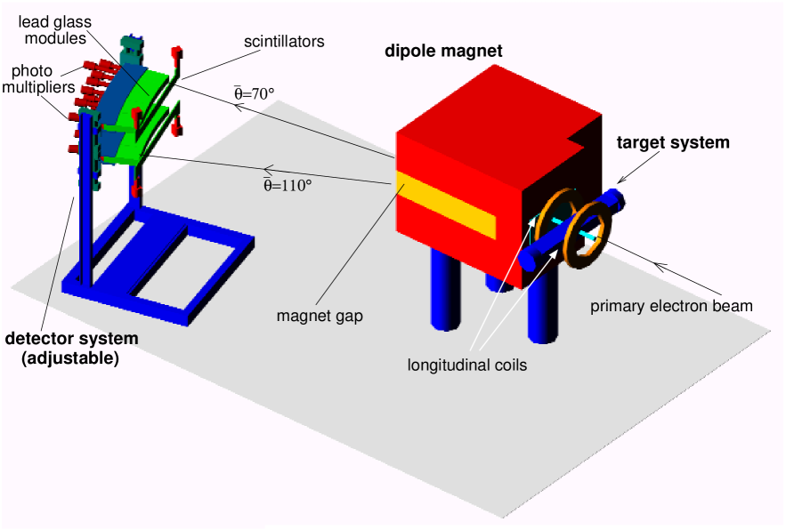
Figure 11: The GDH-Møller-Polarimeter

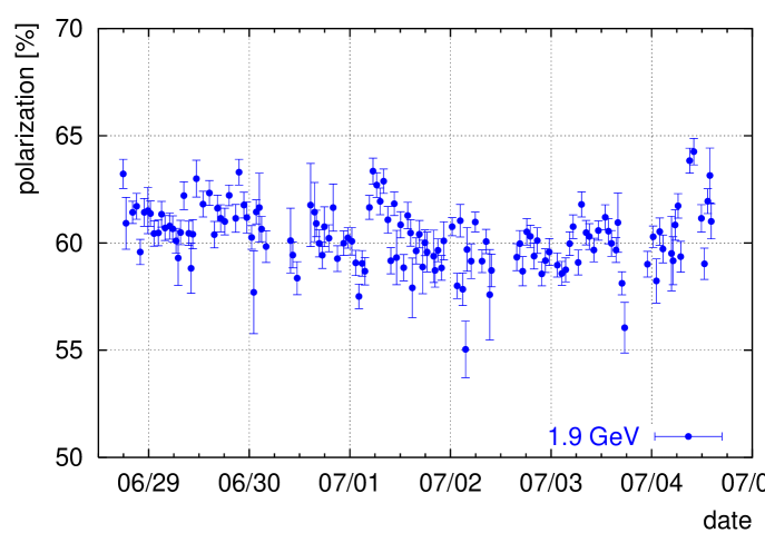
Figure 12: Longitudinal electron polarization monitored during a beam time at 1.9 GeV at Elsa in June/July 2001.

For the GDH-Experiment at Elsa a dedicated Møller polarimeter has been designed [83]. It is situated in the primary electron beam approximately 5 m behind the tagging system (see Fig. 7) and permanently measures the electron polarization during data taking with the GDH-Detector. The polarimeter employs a dipole magnetic spectrometer and lead glass counters to detect both Møller scattered electrons in coincidence (see Fig. 11). The scintillators are used in coincidence with the lead glass detectors to further improve background rejection. A target system consisting of three different pairs of coils provides the field to magnetize Vacoflux foils in all three different space-orientations. This allows to measure all beam polarization components. The variable geometry of the detector system enables adjustments to the kinematic conditions between 0.8 and 3.5 GeV electron beam energy. A large center of mass acceptance of $\overline{\theta}=[65^{o};115^{o}]$ provides the measurement of the longitudinal electron beam polarization for example at 1.9 GeV with a statistical precision of $1~{}\%$ within 10 min ($I_{e}=500$ pA). Fig 12 shows the absolute degree of polarization versus time for a typical run period. The systematic error of the polarization determination with the GDH-Møller-Polarimeter is about 2 % with the dominant source being the uncertainty in the polarization of the magnetic foils. Unprecedented systematic studies of Møller polarimetry as well as direct measurements of the transversal beam polarization components have been performed with this device. The polarimeter has been used extensively to determine the electron beam polarization during accelerator tuning and the data-taking for the verification of the Gerasimov-Drell-Hearn data taking period at Elsa.

4.3.2 Møller polarimetry at MAMI

With a deterministic race track beam polarization transport is substantially less problematic at Mami than at Elsa. Also, the polarization at the bremsstrahlung radiator was always alinged longitudinally. Hence, no dedicated detector components for the identification of Møller electrons were built. Instead, the existing plastic scintillators of the photon tagging system were used for Møller polarimetry, which were read out in coincidence by means of additionally installed electronics. Thus, the tagging spectrometer simultaneously served the purpose of photon energy measurement and as a long-term polarimeter. The acceptance of the Møller polarimeter was limited by the geometry of the vacuum system and by the distance of the poles of the deflecting dipole magnet only.

Three to four hours are needed to achieve a statistical error of 1.5 %. In order to adjust the spin orientation at the beginning of a beam time instead of the Møller polarimeter a fast qualitative examination of the polarization degree was done with a Compton polarimeter [84, 85]. This polarimeter was operated at much higher electron currents than usable during the regular data acquisition.

4.4 Photon beam preparation

4.4.1 Photon polarization

Figure 13: Fraction of electron polarization transfered from the electron beam to the photon beam according to Eq. (89.)

The helicity transfer $h(k)$ connects the degree of circular polarization $P_{\gamma,{\rm circ}}$ transfered to the bremsstrahlung photon beam to the longitudinal electron polarization $P_{e,{\rm long}}$ of the relativistic electron beam [86]:

$$h(k)=\frac{P_{\gamma,{\rm circ}}}{P_{e,{\rm long}}}=\frac{k(3+(1-k))}{3-2(1-k)+3(1-k)^{2}}.$$ (89)

$k=E_{\gamma}/E_{0}$ denotes the fraction of the energy $E_{\gamma}$ of the photon produced by the primary electron with energy $E_{0}$. With the knowledge of the electron beam polarization $P_{e,{\rm long}}$ and the photon energy $E_{\gamma}$ – as determined by the tagging system – the circular polarization $P_{\gamma,{\rm circ}}$ of the energy tagged photon beam can be calculated. Fig. 13 shows that the helicity is transfered most efficiently at high energies. Therefore, the GDH-Tagging-System described in Sec. 4.4.2 only uses the upper third of the bremsstrahlung spectrum for tagging purposes. To cover the energy range from about 680 MeV through 2.9 GeV at Elsa in total 7 primary electron energy settings were used: 1.0, 1.2 , 1.4, 1.9, 2.4, 2.9 and 3.0 GeV. At Mami two energy setting were used to address reactions starting at the pion threshold through 800 MeV: 525 MeV and 855 MeV.

4.4.2 Photon tagging

The GDH-Experiment requires the determination of the absorption cross section of real photons. A common and well established method of generating such a high-energy photon beam utilizes the bremsstrahlung process: A primary electron beam of energy $E_{0}$ impinges on a thin metal foil. At intermediate energies of the scattered electrons the bremsstrahlung process dominates over electron-electron (Møller) scattering, so most electrons that suffer any significant energy loss in the radiator foil radiate a photon which is then used in a real photon experiment.

The residual electron energy $E_{\rm residual}$ is detected by a magnetic spectrometer. Neglecting the small energy transfer to the nucleus this allows to determine the photon energy $E_{\gamma}$:

$$E_{\gamma}=E_{0}-E_{\mathrm{residual}}$$ (90)

The combination of a bremsstrahlung radiator foil and a magnetic spectrometer is called a tagging system. Such systems have become a standard component of real photon experiments in the GeV range [87, 88]. The tagging system provides three essential parameters to the experiment:

• the energy of each photon impinging on the target,

• the flux of photons of a given energy reaching the target and

• the time information of each photon reaching the target.

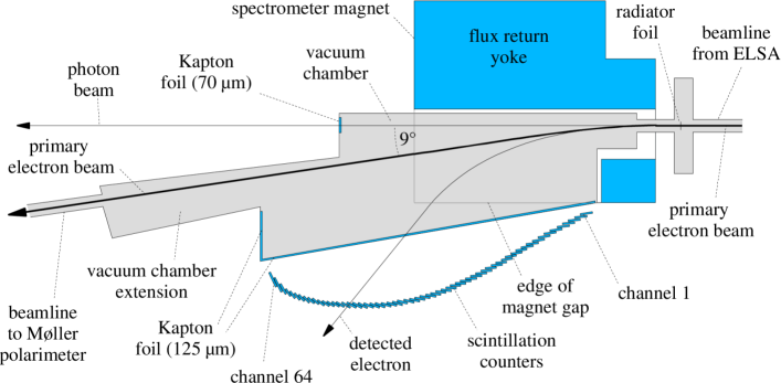
Figure 14: The GDH tagging system at Elsa (top view of the focal plane)

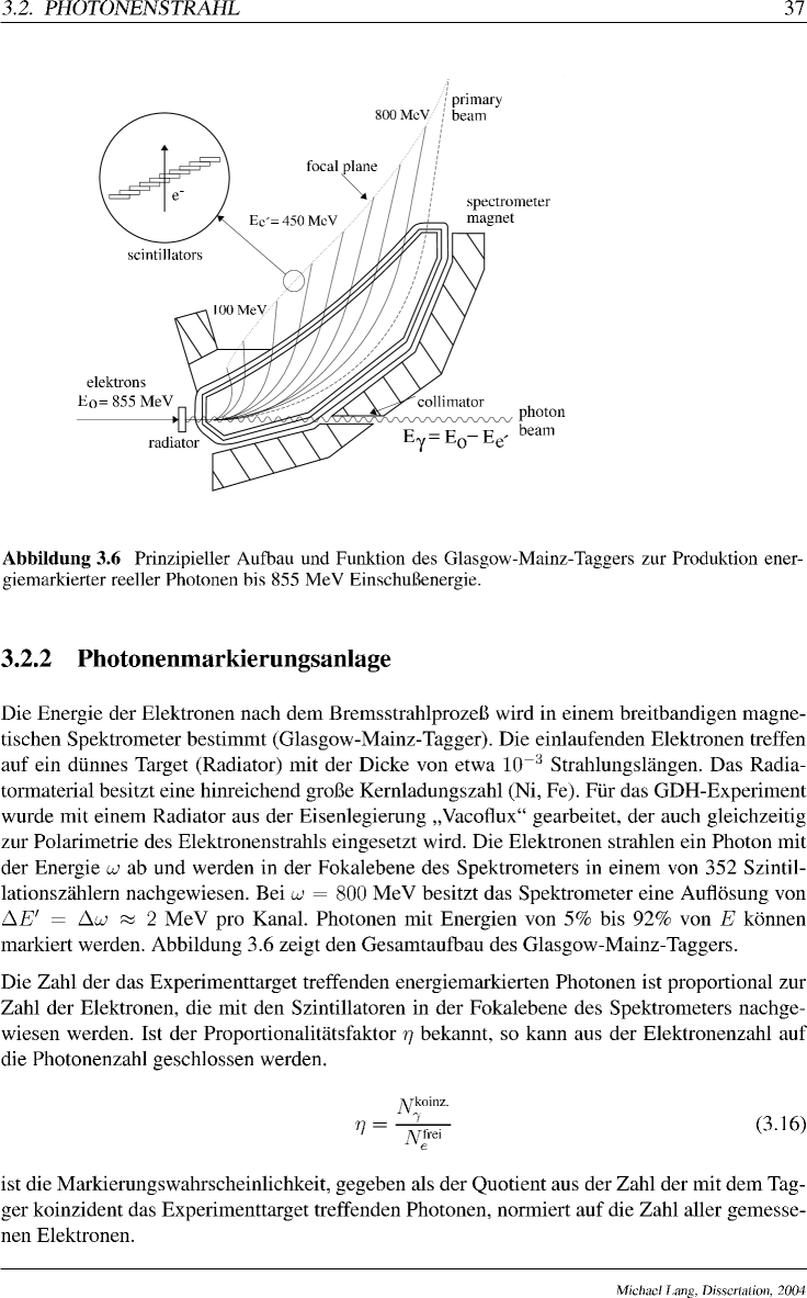
Figure 15: The Glasgow-Mainz tagging system at Mami (top view of the focal plane)

Fig. 14 shows the GDH tagging system operated in Bonn at Elsa [89]. The system consists of a C-type dipole magnet and a hodoscope of 65 scintillation counters which are operated pairwise in coincidence to form 64 tagging channels. Photons can be tagged in a range of 68-97 % of the primary electron energy $E_{0}$. The energy resolution ranges from 0.2 to 0.6 % of $E_{0}$. The time resolution is better than $\sigma=165$ ps. The system was operated at rates up to $5\cdot 10^{6}$ photons/s in the full tagged energy range. The Glasgow-Mainz-Tagger [90] at Mami tags photons in the range of 5-92 % of the primary electron energy and is shown in Fig. 15. Its 352 scintillation counters provide an energy resolution of about 0.2 %

4.4.3 Collimation of the photon beam

Due to the natural divergence of the bremsstrahlung process and the emittance of the primary electron beam the photon beam has to be limited in its divergence and in its transverse size by collimation. The collimators are usually made of a block of lead with a hole in the center, which will be called passive collimators in the following. This type of collimation was used in the GDH setup at Mami.

The collimators have to absorb a sizable proportion of the photons, i.e. 10 % to 90 %, depending on the emittance and the required dimensions of the beam at the hadron target. The following problem arises from passive collimation: A high energy photon which is tagged by the tagging spectrometer may interact with the collimator material and, by pair-production and bremsstrahlung, produces a shower of secondary electrons, positrons and photons. Part of this shower may not be absorbed in the collimator but pass the holes of the collimation system. While the charged particles are deflected away from the beam with a so called sweeping magnet, secondary photons may proceed along with the beam to the target. These photons reach the hadron target with less energy than indicated by the tagging system. With a hadron detector without kinematical over-determination, which cannot determine the photon energy independently of the tagging system, one cannot reject the corresponding events. Additionally, it is imperative to detect and to suppress these secondary photons for a precise determination of the tagging photon definition probability (see Sec. 4.4.4) and of the photon flux.

Since the GDH-Detector at Elsa has only moderate particle identification capabilities this effect has to be considered. Consequently, the active collimation technique described in the following is employed at Elsa. At Mami the central detector has particle identification and tracking. So, this problem is not relevant for the measurements performed at Mami.

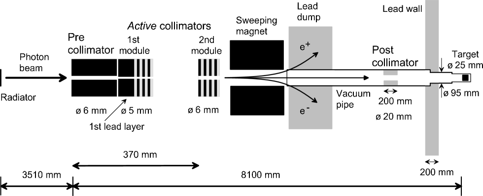
Figure 16: Collimator setup and photon beamline at the GDH-Experiment at Elsa (not to scale).

The idea of an active collimator is to produce a signal each time a photon of the beam hits the collimator and interacts with its material [91]. The photons are identified by their interaction with the collimator medium itself (active collimation). This can be realized with a sandwich of scintillator and lead layers. When the photon hits the collimator medium it produces a shower in which a secondary charged particle gives rise to a signal in the subsequent scintillators. Fig. 16 shows the setup of active collimation and passive shielding for the GDH-Experiment the Elsa as optimized by extensive simulations and test measurements [92]. The geometry with pre-collimation allows to operate this active collimator system at rates of the tagging system exceeding 1 MHz. The collimator system is able to reject secondary low-energy photons with an efficiency of more that 99.9 % for primary photon energies above 500 MeV.

4.4.4 Monitoring the photon definition probability

An important property of a tagged photon beam is the photon definition probability $\eta$ (sometimes also called tagging efficiency). It relates the flux measured in each channel $i$ of the tagging system to the photon flux in the tagged energy range at the experimental target. The precise knowledge of $\eta$ is therefore vital for the correct determination of the photon flux. $\eta_{i}$ for each tagging channel $i$ is defined by:

$$\eta_{i}=\frac{\dot{N}_{{\rm tag},i\wedge{\rm targ}}}{\dot{N}_{{\rm tag},i}}$$ (91)

$\dot{N}_{{\mathrm{tag}},i}$ is the count rate of tagging channel $i$ and $\dot{N}_{{\mathrm{tag}},i\wedge{\mathrm{targ}}}$ is the photon count rate at the experimental target in coincidence with the tagging channel $i$.

In case of the GDH-Experiment at Elsa $\dot{N}_{{\rm tag},i\wedge{\rm targ}}$ was determined by a detector at the photon beam dump. A totally absorbing lead glass Čerenkov counter was used. This detector and its photomultiplier with the corresponding circuitry has been specifically optimized to withstand the high count rates right in the photon beam, even with regular data-taking intensities. This allows a permanent measurement of the photon definition probability during data-taking. The lead glass was exchanged after about every two weeks of time in beam to avoid inefficiencies due to the aging of the glass induced by the beam radiation.

In contrast, at Mami the lead glass Čerenkov counter was only used for a short time about every 24 hours during data-taking to obtain an absolute calibration of $\eta$. For permanent monitoring a detector consisting of 3 scintillators and a copper converter was used. The copper converter was placed between the first two scintillators. The second and third scintillators were operated in anticoincidence to the first one in front of the converter – thus counting the pair creation rate of the photon beam. Under the assumption of constant relative photon definition probabilities of the individual tagging channels this allows to monitor overall drifts of $\eta$.

The systematic uncertainty of the photon definition probability at Mami and at Elsa is less than 2 % for all primary energies.

4.4.5 Beam position monitoring

The photon definition probability and hence the efficiency of the tagging process depend critically on the alignment of the electron and photon beam. At both experimental sites at Elsa and Mami beam profile monitors at the location of the bremsstrahlung radiator were able to determine the electron beam position to within fractions of a millimeter. At Elsa also devices were installed at the photon and electron beam dump as well as at the Møller target. These position monitors are combinations of wires and small detectors. The wires are moved through the beam by stepping motors and the produced secondary particles are detected subsequently.

In addition a camera observing a scintillator following a converter in the photon beam was used for fast beam position monitoring [93] at Elsa and Mami. Due to the more involved electron beam extraction procedure from Elsa its signal was fed back into the accelerator control system to stabilize the beam position and intensity.

With the exception of the monitors at the bremsstrahlung radiators, all these monitors were used online during the data taking.

4.5 Polarized target

One of the reasons, why doubly polarized experiments were not feasible until recently and the GDH Sum Rule has not been measured since the 1960ies is the complexity of the polarized target and the complication of its integration with a detector with almost complete solid angle coverage.

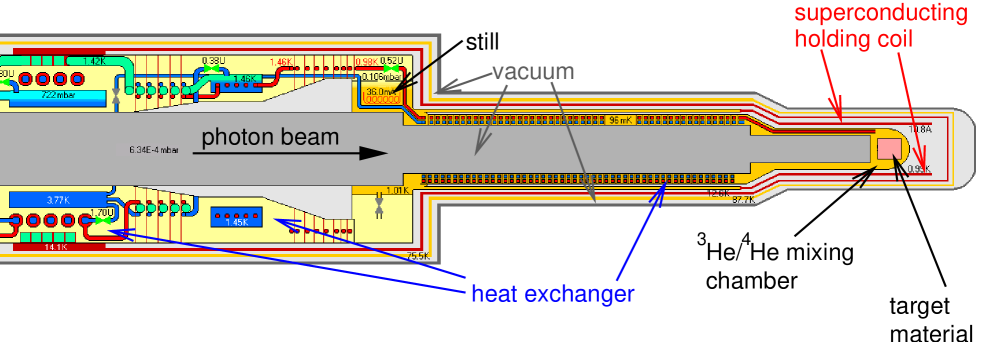
Figure 17: Cryogenic system of the polarized frozen-spin target

For the GDH-Experiment a new “frozen-spin” target has been developed with the ³He/⁴He dilution refrigerator installed horizontally along the beam axis [94]. Frozen-spin mode implies that the polarization is maintained at low temperatures of typically less than 100 mK by only a low magnetic field strength of about 0.5 Tesla. The refrigerator includes an internal superconducting holding coil to provide this longitudinal field for nucleon polarization in the frozen-spin mode. The superconducting wire of this holding coil is wound on the inner cooling shield of the vertical dilution refrigerator. Fig. 17 shows the cryogenic system of the polarized target. The horizontal alignment of the cryostat together with the small internal holding coil minimizes the solid angle affected by these components and distortion of particle tracks due to the magnetic field can be neglected.

The initial polarization of the nucleons is obtained in a slightly different mode. The temperature is raised to a few hundred milli-Kelvin to increase the speed of electron spin relaxation. At the same time a magnet external to the ³He/⁴He cryostat increases the field to about 5 T. This magnet takes the place of the detector during the polarization phase. Detector and polarizing magnet are movable on rails. The proton or deuteron polarization in thermal equilibrium is very small. However, the electrons with a much higher magnetic moment ($\mu_{e}\simeq 660\mu_{p}$) are almost completely polarized. The high polarization of the electrons is transfered to the protons or deuterons by the dynamic nuclear polarization (DNP) technique. Basically, a simultaneous spin flip of an electron and a proton or deuteron transfers the spin polarization from the electrons to the protons. This is achieved applying microwaves of appropriate frequency. A nuclear magnetic resonance (NMR) system measures the degree of polarization of the protons or deuterons.

However, most electrons of the intact molecules of the target material are paired. Only electrons of chemical radicals can be used for this polarization transfer. Butanol (C₄H₉OH) has been used as a polarized proton target at Elsa and at Mami. For the polarized deuteron target at Mami deuterated butanol (C₄D₉OD) was used while lithium-deuteride (⁶LiD) was used for the GDH-Experiment at Elsa. The butanol and deuterated butanol have been chemically prepared for the DNP process with the highly stable free radical porphyrexid ( (CH₃)₂C₃(NO)(NH)(NH)₂ ). The paramagnetic centers in the ⁶LiD were created by irradiating the target material with the 20 MeV electron beam of the Bonn injection linac.

Typical proton polarization values of 70-80 % and deuteron polarization values of 60 % have been obtained. Polarization relaxation times of 200 h (protons) and 100 h (deuterons) have been measured under ideal conditions with butanol. The average deuteron polarization for the ⁶LiD was 27 % with a relaxation time in excess of 1000 h. Fig. 18 shows the typical cycle of polarization buildup, repolarization and relaxation during data-taking periods from the proton.

Figure 18: Proton polarization buildup, repolarization and relaxation during a GDH run at Elsa with a regular butanol target providing polarized protons.

While the interpretation of the polarization as determined with the NMR system for the proton is straight forward the situations is more involved for the deuteron since the nuclear binding modifies the naive picture of two separate nucleons without interaction. For the GDH Sum Rule investigations, however, the individual polarizations of the protons and neutrons are relevant. In the naive picture the proton and the neutron inside the deuteron have parallel spin in the same direction as the deuteron. The dominant correction for the deuteron is the D-state orbital angular configuration [95, 96]. This correction reduces the net nucleon polarization in the deuteron to 93 % of that of the deuteron.

To a first approximation the ⁶Li can be regarded as being composed of a spinless $\alpha$ particle and a proton and a neutron carrying the total spin-1 of the nucleus. In this picture the target material ⁶LiD has almost 50 % of the nucleons’ polarized i.e. a polarization dilution factor of $1/2$. This is to be contrasted to butanol with a dilution factor of $10/74$. Unlike for the deuteron the valence nucleons of the ⁶Li can be found also in a P-state. The net nucleon polarization of the unpaired neutron and proton is 87 % of the ⁶Li polarization [96]. In principle both the polarization of the deuterons and the ⁶Li need to be measured separately. These are however connected by the equal spin temperature (EST) concept [97]. Basically all nuclear species in the target material share the same spin temperature i.e. the Zeeman occupation numbers of each system can be calculated from the respective Brillouin function. Owing this correlation the NMR system was only used to monitor the polarization of the deuterons of the ⁶LiD target.

Small contaminations of the ⁶Li by ⁷Li and of the deuterium by regular hydrogen (¹H) both for the ⁶LiD target as well as for the deuterated butanol have been taken into account [98]. For the two butanol targets also the admixture of the radical prophyrexid dissolved in water representing a 5 % contribution by weight are relevant for the computation of the densities of polarizable nucleons.

The target container length was $l=18.8$ mm for the setup at Mami and $l=28.8$ mm for the setup at Elsa. The diameter of this PTFE container immersed in the ³He/⁴He mixing chamber was 2.0 cm at Mami and 2.6 cm at Elsa. The butanol was prepared in frozen beads (ball shaped) with 2 mm diameter while the ⁶LiD material has the shape of granules (flat blanks). The stacking inside the target container has been determined in detailed investigations [99] to arrive at the target column density.

4.6 Photoabsorption detectors

Two detector arrangements are used to meet the specific requirements for the different energy ranges: The Daphne detector with additional components in forward direction at Mami and the GDH-Detector at Elsa.

Daphne [100] is designed for charged particle detection and for the identification of low multiplicity final states. It is essentially a charged particle tracking detector having a cylindrical symmetry. In addition it has a useful detection efficiency for neutral pions. In forward direction a silicon microstrip device called Midas [101] extends the acceptance for charged particles.

The GDH-Detector [102] has been specifically designed for measurements of total cross sections and is designed for situations where the contributing reaction channels are not well known and extrapolations due to unobserved final states are not advisable. On the other hand, the identification of all individual processes is not required for the determination of the GDH integrand. The concept of the GDH-Detector is to detect at least one reaction product from all possible hadronic processes with almost complete acceptance concerning solid angle and efficiency. The acceptance for hadronic processes is better than 99 %.

Both detection systems have similar components in forward direction (see Figs. 19 and 20). The electromagnetic background is suppressed by about 5 orders of magnitude by means of a threshold Čerenkov detector [102]. The Čerenkov detector is followed by the Star detector component [103] (a scintillator hodoscope to resolve forward polar angles) and the Far-Forward-Wall [102] (a component similar to the central parts of the GDH-Detector) to complete the solid angle coverage.

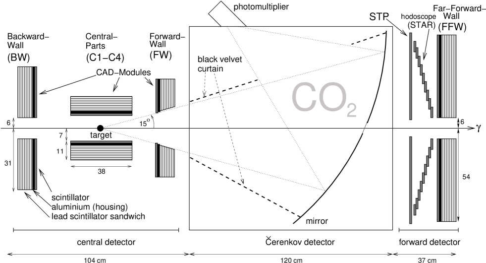
Figure 19: The GDH-Detector used at Elsa for energies above 680 MeV

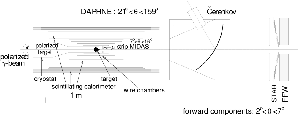
Figure 20: The Daphne detector setup with forward components at Mami for energies below 800 MeV

4.6.1 The GDH-Detector

A cut through of the GDH-Detector [102] is shown in Fig. 19. Apart from the reliable detection of charged particles a high efficiency for neutral decay modes of mesons is necessary in order to increase the total detection probability of the respective photoabsorption channel.

The detection of the charged particles is achieved by plastic scintillators; the decay photons are observed in lead scintillator sandwich detectors behind it. The modules combining these two tasks have been named CAD-Modules. The CAD-Modules are arranged to cover a solid angle of 99.6 %$\ \times\ 4\pi$. The central detector including the backward and forward wall covering the polar angles $15^{\circ}\leq\theta\leq 174^{\circ}$ and also the far-forward wall covering $1.6^{\circ}\leq\theta\leq 15^{\circ}$ are CAD-Modules. In all the hadron detection of the GDH-Detector provides a solid angle acceptance of $4\pi$ – with only 0.02 % solid angle leakage in forward direction and 0.4 % in backward direction.

Charged particles are detected with almost 100 % probability in the front scintillator of the CAD-Modules. The sandwich structure behind is comparable to a calorimeter; however, it was designed with special regard to the efficient detection of low-energetic decay photons and good time resolution. Fig. 9 of Ref. [102] shows that a probability of 88 % was reached for the detection of photons with energies above 50 MeV. Altogether for the detection of the decay of e.g. a $\pi^{0}$-mesons an efficiency of at least 98 % results since the two decay photons independently produce a shower.

Wavelength shifters embedded in plastic light guides are used to minimize the number of photomultipliers needed to read out the CAD-Modules. We have obtained a time resolution of 500 ps even for the 1.2 m² large far-forward CAD-Module and an energy resolution for photon energies above 60 MeV of

$$\frac{\Delta E}{E}=\frac{9.7~{}\%}{\sqrt{E/\mbox{GeV}}}\quad,$$ (92)

has been achieved. The spatial resolution was found to be 15 cm for both charged particles and decay photons.

However, the interactions of photons with the butanol target are predominantly of electromagnetic nature: pair production of electrons and positrons in the Coulomb field of the atomic nuclei and Compton scattering off orbital electrons of the atoms. The angular distribution of this background as obtained in detailed Geant simulations is shown in Fig. 21 in comparison to an important partial channel of the photoabsorption process. One observes that the background has to be suppressed by several orders of magnitude to gain access to the hadronic cross section. However, a separation of the background is possible on the basis of the angular and the momentum distributions which significantly deviate from that of the hadronic final states. Also, it suffices to detect and veto one of the leptons of a created electron-positron pair to veto an electromagnetic process.

Figure 21: Simulated angular distribution of electrons originating from electromagnetic background (normalized to the number of nucleons) with and without Čerenkov veto compared to a typical hadronic process ($\gamma p\to\pi^{+}n$) at 1500 MeV photon energy.

A threshold gas Čerenkov detector installed in forward direction is used to detect particles with a Lorentz factor $\gamma$ larger than a certain threshold value. The Čerenkov threshold needs to be higher than the Lorentz factor the most energetic pions (the lightest hadrons) can reach. The appropriate threshold for the GDH-Experiment at Elsa is $\gamma>22$ . We have used CO₂ with a threshold of $\gamma=36.2$ at standard conditions as a Čerenkov medium. Detailed simulations have shown that a Čerenkov detector with an efficiency of 99.9 % for highly relativistic electrons within a polar half opening angle of 15^∘ is well suited to suppress the background. Fig. 21 illustrates the effectiveness of this veto detector.

The quantity of produced Čerenkov light is proportional to the length of the radiator. A radiator length of 90 cm is sufficient to achieve the required efficiency of 99.9 %. An ellipsoidal mirror with short and long axis of 95.3 cm and 110 cm respectively is inclined by $20^{\circ}$ with respect to the vertical plane and focuses the light onto a photomultiplier (see Fig. 19). The mirror also reflects the ultraviolet part of the Čerenkov light. The reflecting layer consists of aluminum (200 nm thickness), coated with a protective layer of magnesiumfluorid (250 nm thickness, MgF₂) on a Plexiglas carrier (3 mm thickness). To avoid that the photon beam produces background in the mirror of the Čerenkov detector – which obviously would not be suppressed by the Čerenkov veto itself – the mirror has a central hole with 5 cm diameter. The hole is covered by a reflecting aluminum coated mylar foil. In test measurements the Čerenkov detector was found to have indeed an efficiency of 99.990 % for electrons of 1.2 GeV energy. This actually exceeds the required efficiency by one order of magnitude [102].

For the GDH integral a difference of polarized total cross sections is to be measured. This is more difficult than the measurement of an asymmetry as is typically done in polarization experiments because the absolute normalization of all count rates and acceptances is essential. The GDH setup was tested with measurements of unpolarized cross sections [91, 104]. For different primary energies (1.0, 1.4, 1.9, 3.2 GeV) the photoabsorption cross section of carbon (see Fig. 23) and of CH₂ was measured. To verify the capability to measure meaningful differences of cross sections the hydrogen photoabsorption cross section was extracted from the difference of the total cross section of the C-target and of the CH₂-target (see Fig. 22 on the left). The agreement with the literature data [105, 106, 107], the data obtained in the pilot experiment [91, 108] at Phoenics and the matching of the values at the boundaries between primary energy settings shows the reliability of the entire system and of the analysis procedure. The data for carbon are unparalleled in systematic and statistical accuracy.

Figure 22: Top: unpolarized total cross section of carbon; Bottom: unpolarized total cross section of hydrogen obtained as difference of cross sections $(\sigma_{\text{CH}_{2}}-\sigma_{\text{C}})/2$. Both cross sections are compared to published data [105, 106, 107].

4.6.2 The Daphne setup

In the energy range from the pion threshold through 800 MeV, determined by the Mami maximum energy, only a handful of partial channels contribute to the photoabsorption process of the proton and the neutron with the final states $p\,\pi^{0}$, $n\,\pi^{+}$, $n\,\pi^{0}$, $p\,\pi^{0}\pi^{0}$, $n\,\pi^{0}\pi^{0}$, $p\,\pi^{+}\pi^{-}$, $n\,\pi^{+}\pi^{-}$, $p\,\pi^{-}\pi^{0}$, $n\,\pi^{+}\pi^{0}$, $n\,\pi^{+}\pi^{-}$, $n\,\eta$ and $p\,\eta$.

The central component of the detector setup at Mami is the detector Daphne [100]. It is a large-acceptance hadron detector capable of handling few-particle final states. Daphne is roughly cylindrically symmetric and covers the polar angles from $21^{\circ}$ through $159^{\circ}$ which permits particle identification within 94 % of the total solid angle. The detector was essentially built for charged particle identification.

The target in the center of the detector is surrounded by three layers of multiwire proportional chambers with cathode readout. Up to 5 charged particle tracks can be distinguished with these wire chambers. The spatial resolution is of the order of 2 mm which translates into angular resolutions of $\Delta\theta\leq 1^{\circ}$ and $\Delta\phi\leq 2^{\circ}$ (FWHM).

Further outside, the detector consists of 6 scintillator layers. In front of the last three scintillators metal plates (Al, Fe, Pb) are attached which serve as converters for photons. This leads to a useful detection efficiency also for neutral pions of approximately 20 %. The efficiency for charged particles is in the range of 85-95 %. The spatial resolution of the calorimetric component is 10 cm.

The incomplete polar angle acceptance is accounted for by extrapolations based on simulations of the detector and the respective partial channel. For channels with particles in the final state that are not predominantly emitted in forward direction like $\gamma p\to n\pi^{+}$ these corrections are small. So, although we disregard neutron detection in Daphne for obtaining the inclusive results, the systematic error for the total cross section of this partial channel due to the extrapolation is only 2 %. As another example, the total cross section of $\gamma p\to p\pi^{0}$ can be determined from the photons of the $\pi^{0}$ decay. A determination of the differential cross section is complicated due to the forward boost of the proton.

In order to improve the forward angle coverage Daphne is complemented by the detector components Midas [101], Star [103] and the Far-Forward-Wall [102]. A Čerenkov detector similar to the one developed for the GDH-Detector is us as well. Here this threshold Čerenkov veto detector is filled with dry nitrogen and a 5 cm thick layer of aerogel at the entrance window instead of the CO₂ used at Elsa to account for the lower energies at Mami. We will not discuss the forward components in further detail since the results obtained so far are based on the analysis of Daphne only.

Figure 23: Total cross sections per nucleon of hydrogen, deuterium and helium with Daphne at Mami.

Like for the GDH-Detector the setup at Mami has demonstrated its performance by determining unpolarized cross sections with unprecedented quality. Fig. 23 shows several such cross sections [109]. The ³He data are the first of its kind for this nucleus.

5 Results from MAMI and ELSA

5.1 Data analysis

The cross section difference $\Delta\sigma(\nu)=\sigma_{3/2}(\nu)-\sigma_{1/2}(\nu)$ is obtained by:

$$\sigma_{3/2}(\nu)-\sigma_{1/2}(\nu)=\frac{Y_{3/2}(\nu)-Y_{1/2}(\nu)}{\eta(\nu)\cdot f_{\text{t}}\cdot P_{\text{t}}\cdot P_{\text{circ}}(\nu,E_{0})}$$ (93)

with the photon definition probability $\eta$ (see Sec. 4.4.4), the column density of polarized nucleons $f_{t}$, the target polarization $P_{\text{t}}$ (see Sec. 4.5) and the photon beam polarization $P_{\text{circ}}(\nu,E_{o})$. $Y$ is the hadronic yield for the respective spin configurations. This hadronic yield needs further explanation as it is obtained with different methods from the detector setups at Elsa and Mami.

With the GDH-Detector at Elsa obtaining $Y$ is straight forward. For any hadronic reaction at least one particle of the final state is observed. Hence extrapolations to unobserved angles and corrections for incomplete efficiency or acceptance are obsolete. This is also true for the photoabsorption of the neutron. While the detection efficiency for neutrons is moderate only, charged or uncharged mesons are observed with at least 98 % efficiency. Hence, the hadronic yield $Y_{3/2,1/2}(\nu)$ is simply determined by the hadronic count rate of the GDH-Detector in each spin configuration normalized to the photon flux. A hadronic event is identified by a signal in at least one of the 15 detection units of the GDH-Detector provided it is time-correlated with a signal of the tagging system. To avoid double counting, events where two or more units have detected a reaction product are counted with a corresponding weight. Electromagnetic background events are suppressed by the veto detectors. Only very low energy electrons and positrons produced by untagged photons are not identified by the veto detectors. These background events can be suppressed in the analysis by their random character and their lower energy deposition compared to hadronic events. The application of an energy threshold minimizes their effect on the statistical error. A prerequisite for such a handling is the observed negligible fraction of less than $10^{-3}$ of events which occurred as coincident with the tagging system in one module and as randomly correlated in another. Also veto dead-time effects are accounted for.

Obtaining the hadronic yield with Daphne is quite different due to the need to account for acceptance. The largest part of the total hadronic yield $Y$ for the total photoabsorption cross section from Eq. (93) is identified by charged particles detected inside Daphne. Charged pion channels without a neutral pion in the final state need to be corrected for the fraction of events emitted into the angular regions outside the Daphne acceptance. The second largest part is determined from neutral pion events without accompanying charged particle. This number is scaled by the $\pi^{0}$ detection efficiency as determined by detector simulations. The efficiency is finite for all energies and angles of the neutral pion. Hence, no extrapolation is needed for partial channels with at least one $\pi^{0}$ in the final state.

5.2 Systematic studies

Figure 24: Left: relative photon flux difference for the two helicity states of the polarized source at Elsa; Right: Fake asymmetry with unpolarized butanol target with target holding field reversal at Elsa.

In order to assure that the measured polarized cross section differences are generated exclusively by polarized photons scattering off the polarized protons, deuterons or lithium nuclei several systematic studies have been performed. So-called false or fake asymmetries could arise from correlations of the photon flux with the helicity or from the magnetic holding field of the target but also from misconceptions of the trigger logic electronics with respect to processing the helicity signal of the accelerator.

The left hand side of Fig. 24 shows the photon flux difference as determined with the tagging system for the two helicity states of the polarized source at Elsa relative to the total photon flux. One observes that the flux is independent of the helicity. On the right hand side of Fig. 24 the fake asymmetry of the cross section difference for scattering off an unpolarized butanol target is shown i.e. no microwaves for the dynamic nuclear polarization (DNP, see 4.5) have been applied. As expected, even with the reversal of the holding field no significant fake asymmetry arises. The energy dependence of fake asymmetries using unpolarized targets has been studied as well. The resulting upper limits for such asymmetries have been found to be well below 1 $\upmu$b for all energies.

Figure 25: Missing energy spectra for the reaction $\vec{\gamma}\vec{p}\to p\pi^{0}$ at Mami under the assumption that the proton originated from a reaction on a free proton. The spectra are shown for both helicity states and their difference.

Fig. 25 shows the analysis of data taken at Mami with polarized butanol target. The missing energy for the reaction $\vec{\gamma}\vec{p}\to p\pi^{0}$ is plotted with the assumption that the proton originated from a reaction on a free proton i.e. the photon scattered off a polarized hydrogen nucleus. Background contributions from unpolarized carbon and oxygen nuclei of the butanol target are still present in the two separate helicity state diagrams. However, this background cancels nicely in the difference of the two helicity states.

5.3 Spin dependent total photoabsorption cross sections

5.3.1 Results on the proton

Figure 26: Difference of the polarized total photoabsorption cross sections of the proton [110, 9, 111] in comparison to the unpolarized cross section [36, 109].

Fig. 26 shows the final doubly polarized results for $\sigma_{3/2}-\sigma_{1/2}$ on the proton. For comparison also the unpolarized cross section is plotted [36, 109]. These proton data are published in Refs. [110, 9, 111]. The three major resonances known from the unpolarized total cross section are present in the difference as well - they are even more pronounced. A large background of the order of 150 $\upmu$b of helicity insensitive background disappears in the cross section difference. Also an indication of a 4th resonance can be seen in the polarized data (see Sec. 5.4).

To demonstrate that the results for the different energy settings at the two accelerators match each other very well Fig. 27 shows a comparison of all the individual data sets.

Figure 27: Comparison of individual data sets for all energy settings for the polarized total photoabsorption cross section difference of the proton without rebinning and merging.

5.3.2 Results on the deuteron and the neutron

Figure 28: Difference of the polarized total photoabsorption cross section of the deuteron in comparison to the unpolarized cross section.

Fig. 28 shows the results obtained so far for the total photoabsorption cross section of the deuteron again in comparison with the unpolarized cross section [36]. The data from Mami [112, 113] is still under analysis and of preliminary nature. The data were obtained in a pilot run carried out in 1998 at Mami. The high statistics data of the 2003 deuteron run at Mami is currently under analysis. On the other hand, the polarized results from Elsa are of final nature [114].

Qualitatively, the comparison of the polarized to the unpolarized data leads to similar observations like those for the proton. The resonances again appear even more pronounced while a helicity-independent background of the order of 300 $\upmu$b disappears in the cross section difference.

To compute the neutron cross sections from the ⁶LiD data taken at Elsa we have accounted for nuclear effects and chemical admixtures that modify the neutron polarization relative to the measured polarization of the free deuteron (see Sec. 4.5). The simple further decomposition of $\Delta\sigma_{\text{D}}=\Delta\sigma_{\text{p}}+\Delta\sigma_{\text{n}}$ is based on recent calculations [115] which show that coherent contributions present at lower energies can be neglected in the Elsa energy range. The resulting cross section of the neutron based on the Elsa data is shown in Fig. 29. While the response of the neutron at photon energies above 800 MeV in general is very similar to that of the proton one observes a discrepancy of the two cross sections above 1.5 GeV where the proton cross section is headed for a sign change while the neutron data does not show this trend. We will discuss the implications of this further in Secs. 5.5 and 5.6.2.

Figure 29: Comparison of the proton and neutron polarized cross section differences.

5.4 Resonance structure

It is beyond the scope of this review to summarize the wealth of information obtained for the individual resonances with respect to all partial channels studied. More details of the results can be found in [116, 117, 118, 119, 120]. Here, we want to give an overview and the general picture of the current level of understanding of the resonance structure with respect to this data.

Fig. 30 shows the separate helicity contributions to the total cross section. The separated helicity states are obtained by adding resp. subtracting the polarized cross section difference from the unpolarized data. Clearly, most of the resonance strength of the first three resonances originates from the $3/2$ helicity channel. This can be understood intuitively as all major resonances contributing to the cross section have $J\geq 3/2$. The situation appears to be different for the 4th resonance. This structure has not been observed before in unpolarized total cross section data. Here the structure stems at least partially from the drop in the strength of the contribution from helicity $1/2$. This structure might be due to the $F_{35}$ and the $F_{37}$ resonances.

Figure 30: Separate helicity state total cross sections $\sigma_{3/2}$ and $\sigma_{1/2}$ of the proton.

5.4.1 First resonance: $\mathbf{\Delta}(1232)$

In the low energy region around the $\Delta(1232)$-resonance only the two single pion production channels contribute to the total cross section of the proton. This resonance has been studied extensively over decades in pion scattering and pion photoproduction. Mostly unpolarized data have been taken but also single polarization observables (e.g. [121]). Hence, the main multipoles are well determined.

Indeed, Fig. 31 shows that also the doubly polarized data are reasonably well described by the existing parameterizations. Shown for comparison is the parameterization of Maid [122]. This approach incorporates resonance multipole contributions but also Born terms in a unitary isobar model. An alternative parameterization called Said can be found in Ref. [123] which works equally well. The $\Delta$-resonance at the real photon point is primarily of the spin-flip M1 (M${}_{\text{1+}}$) magnetic transition type which dominates the electric quadrupole amplitude E2. One observes that at threshold the E1 (E${}_{\text{0+}}$) contributes only to the $\pi^{+}n$ channel. This can be understood in a simple picture: in the $\pi^{0}p$ system the charge is at the center of gravity and hence the dipole moment is small compared to the $\pi^{+}n$ system. On the other hand the E1 amplitude is the only one that can be excited right at the threshold as it is the one with orbital angular momentum zero of the produced pion nucleon system. For the evaluation of the GDH integral this E1 amplitude is of particular importance (see Sec. 5.6).

Figure 31: Helicity dependence of $\gamma p\to N\pi$ below 450 MeV in comparison to the multipole parameterization Maid [122]. Left: The total cross section difference; Right: The two contributing single pion partial channels.

5.4.2 Second resonance: $\mathbf{D_{13}(1520)}$

With the appearance of additional channels, namely the double pion channels, the parameterizations appear overstrained already. The left hand side of Fig. 32 shows the discrepancy between the preliminary data on single pion production with the parameterization of Maid. The results on $\pi^{0}$ production [117] indicate that the ratio of multipoles M${}_{2-}/$E_2- is rather of the order of 0.56 than the value of 0.45 [36] obtained before.

The double pion production channels $n\pi^{+}\pi^{0}$, $p\pi^{+}\pi^{-}$ and $p\pi^{0}\pi^{0}$ were analyzed separately. The right hand side of Fig. 32 shows the helicity dependent difference of the $\gamma p\to n\pi^{+}\pi^{0}$ channel. Also, models [124, 125] to describe the double pion channels have not yet lead to a satisfactory agreement and the underlying production mechanisms are not fully understood.

Figure 32: Left: Difference of polarized total cross sections and difference of polarized single pion production cross sections in comparison with Maid; Right: Difference of polarized double pion for the channel $\gamma p\to n\pi^{+}\pi^{0}$ in comparison to with two models [124, 125].

5.4.3 Third resonance

Figure 33: Comparison of the polarized total cross sections in the region of the 3rd resonance for the proton and neutron with the single pion production prediction of Maid.

Fig. 33 shows the response of the proton and the neutron to polarized real photons in the region of the third resonance. The proton data appear well described by the single pion photoproduction alone as predicted by Maid. This would indicate that this structure is dominantly generated by single pion production and not by double pion production or other contributions.

For the neutron however, Maid in contrast to the data shows no resonance structure and lies significantly below the experimental results. The neutron data exhibit a structure in the 3rd resonance region similar to the proton data. This could indicate that the scattering mechanism for the neutron is quite different from that of the proton or that the agreement of Maid with the proton data is by chance only and the conclusion of single pion production dominance around 1 GeV is incorrect. This puzzle has to be resolved by future experiments with partial channel resolution.

Figure 34: Separate helicity state total cross sections $\sigma_{3/2}$ and $\sigma_{1/2}$ for the 3rd and the 4th resonance of the proton.

5.4.4 Fourth resonance

Beyond the three resonances well known from the unpolarized total photoabsorption the polarized data exhibit another structure at a photon energy of about 1400 MeV that we may call the fourth resonance. The separate helicity cross sections $\sigma_{3/2}$ and $\sigma_{1/2}$ show a peak difference of about 20 $\upmu$b (see Fig. 34). One might guess that this structure might be due to the excitation of the F₃₅(1905) or F₃₇(1950) resonances. Another explanation could be a cusp affecting $\sigma_{1/2}$ mainly. Further clarification is needed from future experiments to identify the exact origin of the observed new structure.

5.4.5 Comparison with virtual photoabsorption

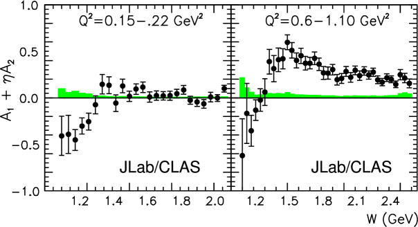
Figure 35: Evolution of the asymmetry $A_{1}$ with photon virtuality $Q^{2}$.

Fig. 35 shows how the asymmetry $A_{1}=\left.\left(\sigma_{1/2}-\sigma_{3/2}\right)\right/\left(\sigma_{1/2}+\sigma_{3/2}\right)\equiv\sigma_{TT^{\prime}}/\sigma_{T}$ evolves from the real photon point. The data in the left panel are from the GDH-Collaboration and the data on the right of Fig. 35 have been taken by the Clas-Collaboration in Hall B at JLab [126]. One observes that apart from the Delta-resonance no higher resonances are visible in the Hall B data. The Delta-resonance looses strength when going to finite $Q^{2}$ and the asymmetry above $W>1.5$ GeV even changes sign.

This dramatic transition already at such a low $Q^{2}\simeq 0.18$ GeV² demonstrates why a verification of the GDH Sum Rule can only be performed at the real photon point as the main contributions to the GDH integral obviously come from the resonance region.

5.5 High-energy behavior

Regge parameterizations incorporate many of the most complicated confinement aspects of strong interactions. This is today’s justification for using Regge approaches even though it was thought to be superseded by QCD.

It has been shown, that the spin averaged total cross section at highest energies is dominated by the Pomeron while at energies right above the resonance region it can be described by the $\rho,\omega$ trajectory [127]:

$$\sigma_{T}(s)\simeq c_{1}\cdot s^{\alpha_{R}(0)-1}+c_{2}\cdot s^{\alpha_{P}(0)-1}$$ (94)

This equation is a simple power law where $\alpha_{R}(0)$ and $\alpha_{P}(0)$ denote the intercepts of the $\rho,\omega$-trajectory and the intercept of the Pomeron-trajectory at Mandelstam $t=0$. All unpolarized total cross sections can be parameterized with the very same values for $\alpha_{R}(0)$ and $\alpha_{P}(0)$ as can be seen in Fig. 36. The values for these intercepts are $\alpha_{R}(0)=0.53$ and $\alpha_{P}(0)=1.08$. Observations of this kind have led to a revival of Regge theory.

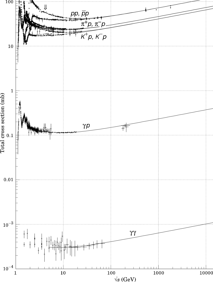
Figure 36: Summary of hadronic, $\gamma p$ and $\gamma\gamma$ total cross sections and a universal Regge fit to the data [128, 36].

We now address the question of the lowest energies where the Regge parameterization may be valid. For the real photoabsorption we have extended the power law fit described above down to low energies and compared it with unpolarized hydrogen data [129]. Fig. 37 shows that indeed the parameterization stemming from data of the several hundreds of GeV range still matches the unpolarized hydrogen cross section down to about 1.2 GeV in photon energy just above the third resonance.

Figure 37: Extrapolation of the high-energy Regge parameterization [127] of unpolarized total cross sections to low energies for real photoabsorption in comparison the experimental data [129].

Figure 38: Comparison of Regge parameterizations with the data from the GDH-Collaboration; Left: Parameterization of DIS data extrapolated to $Q^{2}=0$ by Bianchi and Thomas [130]; Right: Our own parameterization of the GDH data according to Eq. (95).

For polarized real and virtual photoabsorption Bass and Brisudová [131] have shown that the cross section difference can be described by the following Regge behavior:

$$\sigma_{3/2}-\sigma_{1/2}=\left[c_{1}\ s^{\alpha_{a_{1}}-1}\cdot I+c_{2}\ s^{\alpha_{f_{1}}-1}+c_{3}\frac{\ln s}{s}+\frac{c_{4}}{\ln^{2}s}\right]F(s,Q^{2})$$ (95)

where $I$ denotes the isospin of the nucleon and $s$ denotes the square of the center of mass energy. This represents a generalization of the earlier ideas by Close and Roberts [132] as well as by Bass and Landshoff [133]. Bianchi and Thomas have applied Eq. (95) to fit polarized deep inelastic scattering (DIS) data from scattering off protons and deuterons [130]. The extrapolation to the real photon point of their resulting fits for the proton and neutron on the left hand side of Fig. 38 are compared to the high-energy data of the GDH-Collaboration for the proton and neutron. Obviously, this parameterization does not describe the data. This could have two reasons: the extrapolation of this fit from the DIS domain to $Q^{2}=0$ fails or the data still contains structure like resonances that are not well averaged by a Regge parameterization. The latter reason would be a phenomenon unique for the polarized data as the unpolarized data of this energy region are still well described. The extrapolation to the real photon point may fail because of the dramatic transitions observed below $Q^{2}=1$ GeV as seen for example in Figs. 35 and 6.

The logarithmic terms in Eq. (95) are due to Regge cuts and can be neglected at $Q^{2}=0$ [135]. Also for the parameterization of Bianchi and Thomas these terms are insignificant at the real photon point. $F(s,Q^{2})$ simplifies to a constant at the real photon point and can be absorbed into the constants $c_{1}$ and $c_{2}$. $\alpha_{a_{1}}$ and $\alpha_{f_{1}}$ are the Regge intercepts of the respective meson trajectories. Hence in the case of real photons the expression for the Regge behavior simplifies considerably to

$$\sigma_{3/2}-\sigma_{1/2}=\tilde{c}_{1}\ s^{\alpha_{a_{1}}-1}\cdot I+\tilde{c}_{2}\ s^{\alpha_{f_{1}}-1}$$ (96)

The intercept $\alpha_{f_{1}}$ of the $f_{1}$ trajectory is relatively well defined by deep inelastic scattering data and usually found to be about -0.5. The situation is less clear with the intercept of the $a_{1}$ trajectory where the values from different fits range from about -0.2 to +0.9.

The right hand side of Fig. 38 shows the fit of Eq. (96) to both the polarized proton and the polarized neutron data at photon energies above 1.45 GeV via $\tilde{c}_{1}$ and $\tilde{c}_{2}$ as well as via $\alpha_{a_{1}}$ and $\alpha_{f_{1}}$. For the intercepts we obtain $\alpha_{a_{1}}=0.42\pm 0.23$ and $\alpha_{f_{1}}=-0.66\pm 0.22$ which is in reasonable agreement with the findings of DIS fits. The coefficients turn out as $\tilde{c}_{1}=-34.1\pm 5.7~{}\upmu$b and $\tilde{c}_{2}=209.4\pm 29.0~{}\upmu$b where we have used $s$ in units of GeV².

The resulting parameterization of the polarized real photoabsorption is in better agreement with the data than the parameterization of Bianchi and Thomas. This may be by construction of course. The result for the proton indicates a sign change at photon energies above 2 GeV as does the data. The fit below 1.7 GeV deviates from the proton data. This may be a consequence of the fourth resonance structure previously discussed. A fit to the proton data alone does not exhibit this feature [136] which illustrates the significant impact of the inclusion of the neutron data in the fit. The polarized neutron cross section below 1.7 GeV appear slightly lower than the result of the fit. Since there is no polarized data for the neutron at energies above 1.9 GeV it is not clear whether this is a significant discrepancy.

The Regge description of the neutron might also be impaired by a 4th resonance. The statistical error of the fit for the neutron is of the order of 10 $\upmu$b while the departure from the fit of the proton data due to the 4th resonance is also of about this size. Hence, the systematic error due to the ignorance of a possible 4th resonance in the neutron case is not dominant. An extrapolation of the high-energy behavior based on this parameterization appears reasonable. However, a verification of this parameterization with data at higher energies on the proton and also on the neutron would represent a very valuable cross-check.

5.6 The GDH integral and the validity of the GDH Sum Rule

5.6.1 The GDH Sum Rule for the proton

The GDH Sum Rule prediction for the proton amounts to 205 $\upmu$b. In Fig. 39 this prediction is compared to the experimental results. The diagram shows the so-called “running” GDH integral where the infinite integral on the left hand side of Eq. (1) is replaced by an integration up to a certain energy $E_{\text{run}}$:

$$I_{\text{run}}(E_{\text{run}})=\int\limits_{0}^{E_{\text{run}}}\frac{d\nu}{\nu}\left[\sigma_{3/2}(\nu)-\sigma_{1/2}(\nu)\right]$$ (97)

Figure 39: Measured “running” GDH integral up to 2.9 GeV including the threshold contribution.

The experimental data on the proton range from 0.2 through 2.9 GeV in photon energy while the first contribution for photoabsorption at low energies comes from the pion threshold at 0.14 GeV. Between 140 and 200 MeV the two single pion channels $p\pi^{0}$ and $n\pi^{+}$ are the only relevant channels. Since Daphne is not used to detect neutrons alone, the minimum photon energy providing access to the channel $\gamma p\to n\pi^{+}$ is about 200 MeV when the pions have enough energy to enter the detector. As a consequence, also the total polarized photoabsorption is known only above this energy.

In Sec. 5.4.1 we have discussed that at threshold the main contribution has to come from the single E₀₊ multipole. Also, we have seen that the characteristics of the $\Delta$-resonance are well described by the multipole parameterizations Maid and Said, especially with regard to low energies (see Fig. 31). Hence this contribution is very well defined: $-27.5\pm 3~{}\upmu$b is the estimate from Maid [137] and $-28~{}\upmu$b that of Said [138]. Due to the simple nature of the excitation at threshold this can be regarded to be a reliable estimate.

Fig. 39 includes this low-energy contribution from the unmeasured region. One observes how all three major resonances contribute to the running GDH integral. With the contribution of the third resonance at about 900 MeV the integral overshoots the GDH prediction and stays significantly above the GDH Sum Rule value. The value of the GDH sum up to 2.9 GeV is (see Ref. [111])

$$I_{\text{run}}(2.9~{}\text{GeV})=226\pm 5_{\text{stat}}\pm 12_{\text{syst}}\ \upmu\text{b}~{}.$$ (98)

The integrand $\sigma_{3/2}-\sigma_{1/2}$ remains positive from about 230 MeV on up to about 2 GeV as seen in Fig. 26. The sign change of the integrand at higher energies within the measured energy range only marginally improves the agreement of the running GDH integral and the GDH Sum Rule prediction for the proton. However, our Regge parameterization discussed in Sec. 5.5 of the polarized proton and neutron data indicates a negative contribution from the unmeasured high energy region above 2.9 GeV for the proton. We obtain a contribution of -15.3 $\upmu$b to the GDH integral above 2.9 GeV. This fit result from the polarized data almost coincides with those based on DIS data. The parameterization by Bianchi and Thomas [130] gives -14 $\upmu$b and another one by Simula et al. [134] gives -13 $\upmu$b.

With only 3 $\upmu$b the statistical error of the proton extrapolation based on our parameterization is rather small. This is because the errors of the fit parameters are largely anticorrelated. However, the systematic error appears larger as long as it has not been verified with real photon data at higher energies. We estimate it to be 10 $\upmu$b as a conservative estimate considering that the different parameterizations are close together with respect to this high energy contribution.

Including this extrapolation to high energies one obtains for the experimental value of the GDH integral

$$\boxed{\mathbf{I_{\text{run}}(\infty)=212\pm 6_{\text{stat}}\pm 16_{\text{syst}}\ \upmu\text{b}~{}}.}$$ (99)

This is in good agreement with the GDH Sum Rule prediction. The level of precision obtained for the verification of the GDH Sum Rule for the proton is about 8 % including the systematic uncertainties. The dominant sources of the systematic error are uncertainties of beam and target polarization as well as the high energy extrapolation.

This result represents the first verification of the GDH Sum Rule ever!

5.6.2 The GDH Sum Rule for the neutron and the isovector case

The GDH Sum Rule prediction for the neutron is 233 $\upmu$b which is almost 30 $\upmu$b higher than the value for the proton. Moreover, the contribution below 200 MeV due to the $E_{0+}$ amplitude is -50 $\upmu$b [122] i.e. even 22 $\upmu$b lower than for the proton. The cross section difference in the $\Delta$-resonance as predicted by Maid is very similar to that of the proton. The single pion contribution as described by this multipole parameterization in the region of the third resonance is negligible. Taken together this seems to indicate a failure of the GDH Sum Rule for the neutron.

Prior to the experimental results of the GDH-Collaboration a rich literature was addressing the possible failure of the GDH Sum Rule for the isovector case [139, 140, 138]. In the isovector case even the sign of these estimates turns out opposite to the GDH Sum Rule prediction as the following table shows:

	$I^{p}_{\text{GDH}}$	$I^{n}_{\text{GDH}}$	$I^{p-n}_{\text{GDH}}$
GDH Sum Rule	205	233	-28
Karliner [139]	261	183	78
Workman, Arndt [140]	260	192	68
Sandorfi et al. [141]	289	160	129
Drechsel-Krein [142]	261	180	81

The preliminary results [112, 113] from Mami for the polarized cross section up to 800 MeV for the deuteron within the statistical uncertainties are similar to twice the proton cross section. The GDH integral from 200 MeV through 800 MeV for the deuteron amounts to about 420 $\upmu$b. Given the large statistical uncertainties of the data, we will neglect a discussion of nuclear effects for the energy domain from 200 through 800 MeV and simply assume that the deuteron data is the incoherent sum of the proton and neutron. To arrive at an estimate for the neutron we account 200 $\upmu$b for the integral in this energy interval.

The experimental result at Elsa for the GDH integration of neutron data in the energy region 815 - 1825 MeV is $33.9\pm 5.5_{\text{stat}}\pm 4.5_{\text{syst}}\ \upmu\text{b}$ [114]. This contribution previously was assumed to be zero while it turns out to be even larger than for the proton in the respective energy domain. It is one of the two major missing pieces that explain why the validity of the GDH Sum Rule also for the neutron and hence the isovector case is likely.

The other missing piece is the high energy part. Most often this was not accounted for either, like in the analyses summarized in the table. Here we obtain +41 $\upmu$b with our own Regge parameterization as compared to only -15 $\upmu$b for the proton. The statistical error of this contribution to the neutron integral is of the order 10 $\upmu$b. The parameterization of Bianchi and Thomas [106] results in +30 $\upmu$b which is compatible. In total, with the threshold contribution, we obtain an estimate of 225 $\upmu$b for the neutron GDH integral. This is in good agreement with the GDH Sum Rule prediction of 233 $\upmu$b. The systematic and statistical errors are large however.

Considering the isovector case the situation is even more accentuated. The largest contributions to the GDH integral come from the behavior at threshold and at energies above about 1 GeV. The +22 $\upmu$b up to 200 MeV are more than compensated by about -60 $\upmu$b in the range above 800 MeV. The energy range at Mami only gives rise to $\sim$26 $\upmu$b which is compatible with zero given the large statistical and systematic uncertainties of the preliminary data analysis and the ignorance of nuclear effect of the deuteron in the discussion here. The estimate for the total integral for the isovector case amounts to about -10 $\upmu$b. This is to be compared to the GDH Sum Rule prediction of -23 $\upmu$b. Within the large systematic uncertainties this again represents a good agreement. Also, this estimate shows that most of the strength in the isovector case comes from high energies and not from the resonance regime. Since this part has been neglected in most previous estimates for the isovector GDH integral even the resulting sign of these analyses were wrong.

Unlike for the proton, where we are able to present a stringent verification of the GDH Sum Rule at the level of 8 % accuracy, for the time being, we can only give estimates for the neutron and the isovector cases. The further analysis of the Mami data on the deuteron with more statistics and with the detailed treatment of nuclear effects will further clarify the role of the lower resonances. Data especially on polarized deuterium or helium targets are needed at energies above 3 GeV to verify the Regge parameterization.

Today, we have no indication for a failure of the GDH Sum Rule in either case, the proton or the neutron. Especially the relevance of the high energy part above the second resonance has been underestimated in the past for the GDH Sum Rule on the neutron but also for the proton.

6 Future activities related to the GDH Sum Rule

Currently, the analysis of the data of the GDH-Collaboration on the deuteron taken at Mami is being worked on. The results will provide new insight into the resonance structure with respect to isospin but also will help to study nuclear effects with the analyzing power of spin. Also, it should be possible to obtain results with higher precision for the neutron resonance contributions to the GDH Sum Rule. This will move the verification of the GDH Sum Rule on the neutron from the domain of an estimate to a more reliable result.

In order to extend the experimental possibilities of Mami, a fourth microtron acceleration stage is presently under construction, which will increase the electron beam energy to 1.5 GeV. A fourth microtron acceleration stage is presently under construction at Mami. This will increase the electron beam energy to 1.5 GeV and extend the experimental possibilities. As a detector to be used with the tagged photon beam a combination of the Crystal Ball detector [143] and Taps [144] in forward direction will be used. This will allow to study partial channels of the third resonance and part of the forth resonance. Also the improved systematics with respect to the detection of neutral final states will help with measurements of scattering off the deuteron.

Several other experiments are planed that can confirm the findings of the GDH-Collaboration. These experiments use the laser backscattering technique to obtain polarized photons instead of bremsstrahlung produced by polarized electrons. The principal layout of the detection systems are similar to that developed for the GDH-Experiment at Elsa (see Sec. 4.6).

• The Legs facility at BNL uses a polarized HD-target [145] to cover photon energies up to 470 MeV. Very first results have been presented for the tip of the $\Delta$-resonance [146].

• The Graal facility also intends to use the HD-target technique and will cover photon energies up to 550 MeV [147].

• At SPring-8 dynamically polarized PE-foils will be used as a target and the energy coverage is 1.8 – 2.8 GeV [148].

Beyond the energy coverage of the GDH-Collaboration there are experiments planed to extend the measurements to higher energies:

• At JLab a measurement at photon energies from 2.5 through 6 GeV is proposed [149]. A frozen spin target similar to that of the GDH-Collaboration is under development.

• Slac has an approved proposal to measure total cross section asymmetries in the energy regime from 4 to 40 GeV.

Experiments at higher energies will help to verify the Regge parameterization and reduce the systematic error of the extrapolation for the GDH integral.

7 Conclusion

The GDH Sum Rule exclusively relies on fundamental assumptions. These assumptions represent the building blocks of modern physics. We have pointed out that also the “No-subtraction” hypothesis, one of the much questioned steps of its derivation, is of fundamental nature. The validity of the No-subtraction hypothesis is a consequence of unitarity when restrictions to low orders of electromagnetic coupling are avoided. Today no challenge or possible modification of the GDH Sum Rule discussed in the literature appears to be of substantial relevance.

The GDH Sum Rule is a member of a family of so-called super-convergence sum rules. Another prominent member is the Bjorken Sum Rule. The statement of the Bjorken Sum Rule at $Q^{2}\to\infty$ represents the counter piece to the GDH Sum Rule at $Q^{2}=0$. While $Q^{2}\to\infty$ is experimentally only indirectly accessible by means of a QCD evolution the GDH Sum Rule is measurable directly at the real photon point using bremsstrahlung photons. The connection of the two sum rules by means of the generalized GDH Sum allows to study the transition from partonic degrees of freedom to the domain of hadronic interactions. It turns out that this transition in terms of the GDH Sum in the range $0~{}\text{GeV}^{2}\leq Q^{2}\leq 1~{}\text{GeV}^{2}$ is quite dramatic and exceeds the variations found at higher $Q^{2}$.

The GDH-Experiment was performed at two accelerators, Elsa and Mami, to cover a very wide energy range from pion threshold to the onset of the Regge regime. Extensive polarimetry of the beam was done to keep this source of systematic errors low. Tagging systems with sub-percent energy resolution were used to prepare the photon beams. A polarized solid state target integrated in a horizontal cryostat was used minimizing the impact on solid angle coverage. Two detectors designed for the two energy regions at Elsa and Mami with high solid angle coverage have determined the polarized total photoabsorption cross sections.

The results from the GDH-Collaboration on the polarized photoabsorption show that apart from the lowest lying $\Delta$-resonance the structure of the nucleon’s response is largely not understood. The data verify the Gerasimov-Drell-Hearn Sum Rule for the proton at the level of 8 % including systematic errors of the extrapolation to unmeasured energy regions. The GDH Sum Rule for the neutron and the isovector case also appear to be valid. Here the high energy part above 1 GeV in photon energy plays an important role that was underestimated in previous attempts that found discrepancies to the sum rule prediction.

More precise results on the deuteron and the neutron can be expected from the GDH-Experiment at Mami when the data already taken are analyzed. Future experiments on total photoabsorption at photon energies above 3 GeV will reduce the systematic error of the extrapolation to the high-energy domain.

Acknowledgements
 
I am indebted to Gisela Anton for her continuous and steadfast support and advise and her encouragement throughout the whole GDH project and many years of challenges.

Also, I am grateful to Berthold Schoch for initially suggesting the investigation of the GDH Sum Rule and for his support for the GDH-Collaboration in general and for me in pursuing the experiment in particular.

I wish to thank my colleagues of the GDH-Collaboration who all contributed to the great success of the experiment; in particular, Hans-J rgen Arends, J rgen Ahrens, Andrea Bock, Wolter von Drachenfels, Hartmut Dutz, Frank Frommberger, Peter Grabmayr, Paolo Pedroni, Jochen Krimmer, Werner Meyer, Thilo Michel, Jakob Naumann, Markus Sauer, Thorsten Speckner, Robert Van de Vyver and G nter Zeitler.

It is a pleasure to thank Horst Rollnik for numerous very valuable and illuminative discussions and for sharing his profound knowledge of theoretical physics. For several instructive conversations on aspects of the derivation of the GDH sum rule, I am grateful to Robert L. Jaffe. Several lively and challenging discussions with Ralf Panf rder and Steven Bass are gratefully acknowledged.

References

- [1] S.B. Gerasimov, Sov. J. Nucl. Phys. 2 (1966) 430.
- [2] S.D. Drell and A.C. Hearn, Phys. Rev. Lett. 16 (1966) 908.
- [3] S.B. Gerasimov, Yadern. Fiz. 2 (1965) 598.
- [4] M. Hosoda and K. Yamamoto, Prog. Theor. Phys. 36 (1966) 425.
- [5] G. Barton and N. Dombey, Phys. Rev. 162 (1967) 1520.
- [6] J.R. Ellis and R.L. Jaffe, Phys. Rev. D9 (1974) 1444.
- [7] E80 Collaboration, G. Baum et al., Phys. Rev. Lett. 51 (1983) 1135.
- [8] European Muon Collaboration, J. Ashman et al., Nucl. Phys. B328 (1989) 1.
- [9] GDH Collaboration, H. Dutz et al., Phys. Rev. Lett. 91 (2003) 192001.
- [10] GDH Collaboration, K. Helbing, Nucl. Phys. Proc. Suppl. 105 (2002) 113.
- [11] D. Drechsel and L. Tiator, Ann. Rev. Nucl. Part. Sci. 54 (2004) 69, nucl-th/0406059.
- [12] S.D. Bass, (2004), hep-ph/0411005.
- [13] D.A. Dicus and D.R. Palmer, Phys. Rev. D6 (1972) 720.
- [14] M. Jacob and G.C. Wick, Ann. Phys. 7 (1959) 404.
- [15] H. Rollnik and P. Stichel, Springer Tracts in Modern Physics 79 (1976) 1.
- [16] B.H. Kellett, Phys. Rev. D7 (1973) 115.
- [17] M. Gell-Mann, M.L. Goldberger and W.E. Thirring, Phys. Rev. 95 (1954) 1612.
- [18] M.L. Goldberger, Phys. Rev. 97 (1955) 508.
- [19] W. Thirring, Phil. Mag. 41 (1950) 1193.
- [20] F.E. Low, Phys. Rev. 96 (1954) 1428.
- [21] M. Gell-Mann and M.L. Goldberger, Phys. Rev. 96 (1954) 1433.
- [22] M. Gell-Mann, Nuovo Cimento Suppl. 2 4 (1956) 848.
- [23] A.M. Baldin, Nucl. Phys. 18 (1960) 310.
- [24] R. Pantförder, Investigations on the foundation and possible modifications of the Gerasimov-Drell-Hearn sum rule, PhD thesis, Bonn University, 1998, hep-ph/9805434.
- [25] K. Kawarabayashi and M. Suzuki, Phys. Rev. 152 (1966) 1383.
- [26] A. Khare, Prog. Theor. Phys. 53 (1975) 1798.
- [27] L.N. Chang, Y.g. Liang and R.L. Workman, Phys. Lett. B329 (1994) 514, hep-ph/9403286.
- [28] R. Pantförder, H. Rollnik and W. Pfeil, Eur. Phys. J. C1 (1998) 585, hep-ph/9703368.
- [29] A. Harindranath, (1994), hep-ph/9410390.
- [30] H.D.I. Abarbanel and M.L. Goldberger, Phys. Rev. 165 (1968) 1594.
- [31] S.M. Roy and V. Singh, Phys. Rev. Lett. 21 (1968) 861.
- [32] T.P. Cheng, Phys. Rev. 184 (1969) 1805.
- [33] G.E. Uhlenbeck and S. Goudsmith, Nature 117 (1926) 264.
- [34] D.P.A. M., Proc. Roy. Soc. A117 (1928) 610.
- [35] J.S. Schwinger, Phys. Rev. 82 (1951) 664.
- [36] Particle Data Group, S. Eidelman et al., Phys. Lett. B592 (2004) 1.
- [37] T.L. Trueman, Phys. Rev. Lett. 17 (1966) 1198.
- [38] A.H. Mueller and T.L. Trueman, Phys. Rev. 160 (1967) 1306.
- [39] V. de Alfaro et al., Phys. Lett. 21 (1966) 576.
- [40] M. Froissart, Phys. Rev. 123 (1961) 1053.
- [41] G. Altarelli, N. Cabibbo and L. Maiani, Phys. Lett. B40 (1972) 415.
- [42] S. Gerasimov and J. Moulin, Nucl. Phys. B98 (1975) 349.
- [43] S.J. Brodsky and I. Schmidt, Phys. Lett. B351 (1995) 344, hep-ph/9502416.
- [44] L.D. Landau, Dokl. Akad. Nauk USSR 60 (1948) 207.
- [45] C.N. Yang, Phys. Rev. 77 (1950) 242.
- [46] W. Drechsler, Fortsch. Phys. 18 (1970) 305.
- [47] S.D. Bass, Acta Phys. Polon. B34 (2003) 5893, hep-ph/0311174.
- [48] S.D. Bass, private communication, 2004.
- [49] H.D.I. Abarbanel et al., Phys. Rev. 160 (1967) 1329.
- [50] R.E. Cutkosky, J. Math. Phys. 1 (1960) 429.
- [51] R. Blankenbecler, Phys. Rev. 122 (1961) 983.
- [52] L.F. Cook and B.W. Lee, Phys. Rev. 127 (1962) 283.
- [53] H.C. Baker, E.Y.C. Lu and L.E. Wood, Phys. Rev. D2 (1970) 3031.
- [54] H. Rollnik, 2005, private communication.
- [55] P.D.B. Collins and E.J. Sqires, Springer Tracts in Modern Physics 45 (1968).
- [56] J. Blumlein and N. Kochelev, Nucl. Phys. B498 (1997) 285, hep-ph/9612318.
- [57] J.D. Bjorken, Phys. Rev. 148 (1966) 1467.
- [58] E.D. Bloom et al., Phys. Rev. Lett. 23 (1969) 930.
- [59] P. Mohr and B. Taylor, J. Phys. Chem. Reference Data 28 (1999) 1713, CODATA Recommended Values of the Fundamental Physical Constants: 1998.
- [60] HERMES Collaboration, K. Ackerstaff et al., Phys. Lett. B464 (1999) 123, hep-ex/9906035.
- [61] Spin Muon Collaboration (SMC), D. Adams et al., Phys. Rev. D56 (1997) 5330, hep-ex/9702005.
- [62] E80 Collaboration, M.J. Alguard et al., Phys. Rev. Lett. 37 (1976) 1261.
- [63] E80 Collaboration, M.J. Alguard et al., Phys. Rev. Lett. 41 (1978) 70.
- [64] E143 Collaboration, K. Abe et al., Phys. Rev. Lett. 74 (1995) 346.
- [65] E143 Collaboration, K. Abe et al., Phys. Rev. Lett. 75 (1995) 25.
- [66] R.L. Jaffe and A. Manohar, Nucl. Phys. B337 (1990) 509.
- [67] HERMES Collaboration, A. Airapetian et al., (2004), hep-ex/0407032.
- [68] COMPASS Collaboration, S. Hedicke, Prog. Part. Nucl. Phys. 50 (2003) 499.
- [69] L.C. Bland, AIP Conf. Proc. 747 (2005) 63, hep-ex/0412009.
- [70] D. Drechsel, S.S. Kamalov and L. Tiator, Phys. Rev. D63 (2001) 114010, hep-ph/0008306.
- [71] X.D. Ji, Phys. Lett. B309 (1993) 187, hep-ph/9307303.
- [72] X.D. Ji and J. Osborne, J. Phys. G27 (2001) 127, hep-ph/9905410.
- [73] V. Bernard, T.R. Hemmert and U.G. Meissner, Phys. Lett. B545 (2002) 105, hep-ph/0203167.
- [74] X.D. Ji, C.W. Kao and J. Osborne, Phys. Lett. B472 (2000) 1, hep-ph/9910256.
- [75] HERMES Collaboration, A. Airapetian et al., Eur. Phys. J. C26 (2003) 527, hep-ex/0210047.
- [76] E143 Collaboration, K. Abe et al., Phys. Rev. Lett. 78 (1997) 815, hep-ex/9701004.
- [77] CLAS Collaboration, R. Fatemi et al., Phys. Rev. Lett. 91 (2003) 222002, nucl-ex/0306019.
- [78] Y. Prok, (2005), Proceedings of the GDH 2004.
- [79] K.H. Steffens et al., Nucl. Instrum. Meth. A325 (1993) 378.
- [80] W. Hillert, M. Gowin and B. Neff, Prepared for 14th International Spin Physics Symposium (SPIN 2000), Osaka, Japan, 16-21 Oct 2000.
- [81] S. Nakamura et al., Nucl. Instrum. Meth. A411 (1998) 93.
- [82] M. Hoffmann et al., Prepared for 14th International Spin Physics Symposium (SPIN 2000), Osaka, Japan, 16-21 Oct 2000.
- [83] T. Speckner et al., Nucl. Instrum. Meth. A519 (2004) 518.
- [84] I. Drescher, Master’s thesis, Mainz, 1995.
- [85] B. Fürst, Master’s thesis, Mainz, 1998.
- [86] H. Olsen and L.C. Maximon, Phys. Rev. 114 (1959) 887.
- [87] P. Detemple et al., Nucl. Instrum. Meth. A321 (1992) 479.
- [88] D.I. Sober et al., Nucl. Instrum. Meth. A440 (2000) 263.
- [89] J. Naumann et al., Nucl. Instrum. Meth. A498 (2003) 211.
- [90] I. Anthony et al., Nucl. Instrum. Meth. A301 (1991) 230.
- [91] K. Helbing, Messung von totalen Photoabsorptionsquerschnitten mit dem GDH-Detektor, PhD thesis, Bonn University, 1997.
- [92] G. Zeitler et al., Nucl. Instrum. Meth. A459 (2001) 6.
- [93] J. Krimmer, P. Grabmayr and M. Sauer, Nucl. Instrum. Meth. A481 (2002) 57.
- [94] C. Bradtke et al., Nucl. Instrum. Meth. A436 (1999) 430.
- [95] W. Melnitchouk, G. Piller and A.W. Thomas, Phys. Lett. B346 (1995) 165, hep-ph/9501282.
- [96] O.A. Rondon, Phys. Rev. C60 (1999) 035201.
- [97] A. Abragam and M. Goldman, Rept. Prog. Phys. 41 (1978) 395.
- [98] J. Ball et al., Nucl. Instrum. Meth. A498 (2003) 101.
- [99] C.C. Rohlof and H. Dutz, Nucl. Instrum. Meth. A526 (2004) 126.
- [100] G. Audit et al., Nucl. Instrum. Meth. A301 (1991) 473.
- [101] S. Altieri et al., Nucl. Instrum. Meth. A452 (2000) 185, nucl-ex/9911001.
- [102] K. Helbing et al., Nucl. Instrum. Meth. A484 (2002) 129.
- [103] M. Sauer et al., Nucl. Instrum. Meth. A378 (1996) 143.
- [104] T. Michel, Messung von totalen Photoabsorptionsquerschnitten als Vorbereitung des GDH-Experiments an ELSA, PhD thesis, Erlangen University, 2001.
- [105] T.A. Armstrong et al., Nucl. Phys. B41 (1972) 445.
- [106] N. Bianchi et al., Phys. Lett. B309 (1993) 5.
- [107] V. Muccifora et al., Phys. Rev. C60 (1999) 064616, nucl-ex/9810015.
- [108] M. Sauer, Inklusive Messung von Wirkungsquerschnitten der totalen Photoabsorption am Proton und Neutron als Vorbereitung für das GDH-Experiment, PhD thesis, Tübingen University, 1998.
- [109] M. MacCormick et al., Phys. Rev. C53 (1996) 41.
- [110] GDH Collaboration, J. Ahrens et al., Phys. Rev. Lett. 87 (2001) 022003, hep-ex/0105089.
- [111] GDH Collaboration, H. Dutz et al., Phys. Rev. Lett. 93 (2004) 032003.
- [112] T. Rostomyan, PhD thesis, Gent University, 2005, in preparation.
- [113] O. Jahn, (2004), Proceedings of the GDH 2004 symposium, World Scientific Publishing Company.
- [114] GDH, H. Dutz et al., Phys. Rev. Lett. 94 (2005) 162001.
- [115] H. Arenhovel, A. Fix and M. Schwamb, Phys. Rev. Lett. 93 (2004) 202301, nucl-th/0407058.
- [116] GDH Collaboration, J. Ahrens et al., Phys. Rev. Lett. 84 (2000) 5950.
- [117] GDH Collaboration, J. Ahrens et al., Phys. Rev. Lett. 88 (2002) 232002, hep-ex/0203006.
- [118] GDH Collaboration, J. Ahrens et al., Phys. Lett. B551 (2003) 49.
- [119] GDH Collaboration, J. Ahrens et al., Eur. Phys. J. A17 (2003) 241.
- [120] GDH Collaboration, J. Ahrens et al., Eur. Phys. J. A21 (2004) 323.
- [121] H. Dutz et al., Nucl. Phys. A601 (1996) 319.
- [122] D. Drechsel et al., Nucl. Phys. A645 (1999) 145, nucl-th/9807001.
- [123] R.A. Arndt, I.I. Strakovsky and R.L. Workman, Phys. Rev. C53 (1996) 430, nucl-th/9509005.
- [124] J. Nacher and E. Oset, Nucl. Phys. A697 (2002) 372.
- [125] H. Holvoet, PhD thesis, Gent University, 2001.
- [126] V.D. Burkert, Mod. Phys. Lett. A18 (2003) 262, hep-ph/0211185.
- [127] A. Donnachie and P.V. Landshoff, Phys. Lett. B296 (1992) 227, hep-ph/9209205.
- [128] Courtesy of the Compas group, IHEP, Protvino, Russia, 1998.
- [129] T.A. Armstrong et al., Phys. Rev. D5 (1972) 1640.
- [130] N. Bianchi and E. Thomas, Phys. Lett. B450 (1999) 439, hep-ph/9902266.
- [131] S.D. Bass and M.M. Brisudova, Eur. Phys. J. A4 (1999) 251, hep-ph/9711423.
- [132] F.E. Close and R.G. Roberts, Phys. Lett. B336 (1994) 257, hep-ph/9407204.
- [133] S.D. Bass and P.V. Landshoff, Phys. Lett. B336 (1994) 537, hep-ph/9406350.
- [134] S. Simula et al., Phys. Rev. D65 (2002) 034017, hep-ph/0107036.
- [135] J. Kuti, (1997), Proceedings of Erice School 1995 on The spin structure of the nucleon (World Scientific) and private communication.
- [136] GDH Collaboration, K. Helbing, AIP Conf. Proc. 675 (2003) 33.
- [137] L. Tiator, Proceedings of the GDH 2002 symposium, World Scientific Publishing Company.
- [138] R.A. Arndt et al., Phys. Rev. C66 (2002) 055213, nucl-th/0205067.
- [139] I. Karliner, Phys. Rev. D7 (1973) 2717.
- [140] R.L. Workman and R.A. Arndt, Phys. Rev. D45 (1992) 1789.
- [141] A.M. Sandorfi, M. Khandaker and C.S. Whisnant, Phys. Rev. D50 (1994) 6681.
- [142] D. Drechsel and G. Krein, Phys. Rev. D58 (1998) 116009, hep-ph/9808230.
- [143] A. Badala et al., Nucl. Instrum. Meth. A306 (1991) 283.
- [144] A. Marin et al., Nucl. Instrum. Meth. A417 (1998) 137.
- [145] X. Wei et al., Nucl. Instrum. Meth. A526 (2004) 157.
- [146] LEGS SPIN Collaboration, A.M. Sandorfi et al., AIP Conf. Proc. 675 (2003) 651.
- [147] GRAAL Collaboration, F. Renard, Proceedings of the GDH 2000 symposium, World Scientific Publishing Company.
- [148] T. Iwata, Proceedings of the GDH 2000 symposium, World Scientific Publishing Company.
- [149] CLAS Collaboration, D.I. Sober et al., Proceedings of the NStar 2002 workshop, World Scientific Publishing Company.