Isotopic Production Cross Sections in Proton-Nucleus Collisions at 200 MeV

Abstract

Intermediate mass fragments (IMF) from the interaction of ²⁷Al, ⁵⁹Co and ¹⁹⁷Au with 200 MeV protons were measured in an angular range from 20 degree to 120 degree in the laboratory system. The fragments, ranging from isotopes of helium up to isotopes of carbon, were isotopically resolved. Double differential cross sections, energy differential cross sections and total cross sections were extracted.

I Introduction

Studies of spallation processes, both experimental and theoretical, are numerous. One reason for this may be the importance of knowledge of cross sections and reaction mechanisms for our understanding of cosmic rays Auger39 ; Brown49 ; Powell59 ; Fields00 ; Biermann01 ; Hoerandel01 ; Nolfo01 and the production of cosmogenic radionuclides Michel96 ; Waddington99 , and the process of neutron production in spallation sources. Recent reviews of the process can be found in Refs Huefner85 ; Silberberg90 . Most of the experimental data exist in the range above 1 GeV which is important for spallation neutron source construction and the understanding of very high energy cosmic rays. However, the energy of the maximum abundance of protons in cosmic rays is around 200 MeV Austin81 ; Simpson83 . We measured intermediate mass fragments at a proton beam energy of 200 MeV incident on three targets spanning the periodic table, namely, ²⁷Al, ⁵⁹Co and ¹⁹⁷Au. These data complement previous cross sections for proton, deuteron and tritium emission on ²⁷Al and ¹⁹⁷Au Didelez82 ; Machner84 . The cross sections given there for ³He and $\alpha$-particles are too small when compared to systematics Kalbach87 ; Kalbach88 . They were measured with a set up different to that used for the hydrogen isotopes and might be low by a factor of 4. We will come back to this point. They also complement data for a silver target taken at proton energies close by Green80 ; Yennello90 .

II Experiments

The experiment was performed at the separated-sector cyclotron facility of iThemba labs. A detailed description of the layout of the facility and equipment is given in Ref. Pilcher89 and references therein. The beam of 200 MeV was focused to a spot size of less than 2 $\times$ 2 mm at the target center of a 1.5 m diameter scattering chamber. Great care was taken to minimize the halo of the incident proton beam by focusing the beam through a 3 mm diameter hole in a ruby scintillator target. The targets were self supporting foils with thicknesses of 2.9 mg/cm², 1.0 mg/cm² and 4.0 mg/cm² for ²⁷Al, ⁵⁹Co and ¹⁹⁷Au, respectively. The target materials had purity of 99.9$\%$. A possible (invisible) oxidation of the surface in case of the aluminum target leads to a negligible amount of oxygen. Fragments were measured with a telescope consisting of an active collimator followed by three silicon detectors with thicknesses of 50 $\mu$m, 150 $\mu$m and 1 mm. The solid angle of the telescope was 2.2 msr. Another 1 mm thick detector vetoed penetrating hydrogen and helium isotopes. The detectors were calibrated with radioactive sources and a precision pulse generator. In order to reduce electronic noise they were cooled to a few degrees with chilled water. Detection angles were from 20^oto 120^o. The opening angle of the collimator resulted in an angle uncertainty of $\pm 2.2$^o. The incident proton flux was measured by a beam dump Faraday cup.

The $\Delta E-E$ method was used for particle identification. A linearized particle identification quantity, $PI$, was obtained from the energy-range relation, given by

$$PI=\left[\left(E_{1}+E_{2}\right)^{b}-E_{2}^{b}\right]/d_{1}$$ (1)

if the particle is stopped in the second detector. $E_{i}$ denotes the energy deposited in the i-th detector and $d$ is the detector thickness. If the particle is stopped in the third detector one has the relation

$$PI=\left[\left(E_{1}+E_{2}+E_{3}\right)^{b}-E_{3}^{b}\right]/(d_{1}+d_{2}).$$ (2)

Furthermore

$$mZ^{2}\propto PI.$$ (3)

with $m$ the fragment mass and $Z$ the charge number.

Figure 1: Mass distributions from the interaction of 200 MeV protons with ${}^{59}Co$ measured at 20^o.

For the exponent a value $b=1.73$ was used. As an example a mass distribution, obtained by dividing the ranges in the PI-spectrum by $Z^{2}$, is shown in Fig. 1 for the case of cobalt. Hydrogen isotopes fulfilling the energy conditions (1) or (2) have the largest yield, but are not considered here. Good isotope separation is visible up to boron. In the case of the gold target even carbon fragments could be resolved.

The counting rate was then converted to cross sections. The following systematic errors contribute to the total uncertainty. The target thicknesses are known with typically 10$\%$ uncertainty. The incident flux was measured with 2$\%$ uncertainty, while the solid angle, electronic dead time correction and energy calibration were estimated to contribute in total to less than 2$\%$. The emission angles are uncertain to $\pm 2.2$^o. The error bars in the figures show only the statistical uncertainty.

In Figs 2– 9 double differential cross sections are shown for IMFs ranging from ${}^{4}He$ to ${}^{10}B$. The statistics get poorer with increasing mass number.

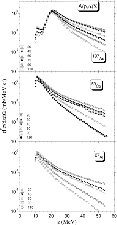
Figure 2: Energy spectra of $\alpha$ particles for the given angles and the given targets.

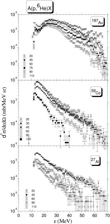
Figure 3: Same as Fig. 2 but for ⁶He emission.

Figure 4: Same as Fig. 2 but for ⁶Li emission.

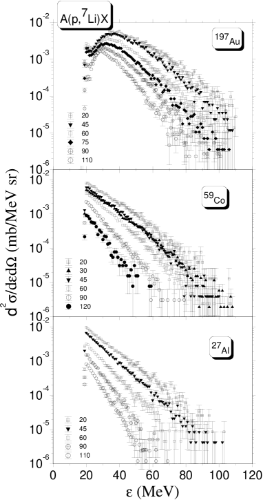
Figure 5: Same as Fig. 2 but for ⁷Li emission.

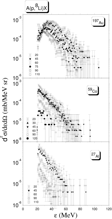
Figure 6: Same as Fig. 2 but for ⁸Li emission.

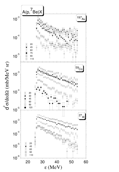
Figure 7: Same as Fig. 2 but for ⁷Be emission.

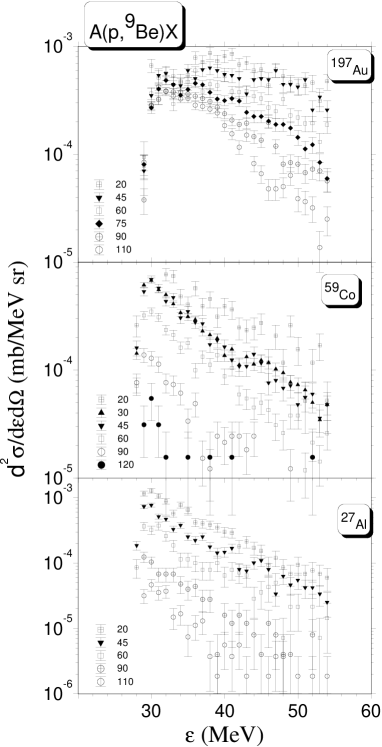
Figure 8: Same as Fig. 2 but for ⁹Be emission.

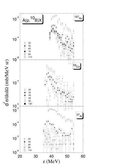
Figure 9: Same as Fig. 2 but for ¹⁰B emission.

The IMF spectra in the case of the gold target show the effect of the Coulomb barrier: a maximum which is in most cases close to 10 MeV$\times Z$ with $Z$ the fragment charge number. In the case of the cobalt target this is just at the detection threshold which is given by the thickness of the first $\Delta E$ detector. For aluminum the Coulomb barrier is below our detection range. In case of the gold target a second component shows up. This is emission below the Coulomb barrier of a gold-like system. It is obviously emission from a system with a much smaller Coulomb barrier. Unfortunately, the first $\Delta E$ detector is too thick to study such a component in the case of the other targets. Such a component can be explained as emission from fission fragments which in the case of lighter target nuclei are not as frequent as in the case of gold and was also seen in the emission of low energy protons following $\bar{p}$ absorption on uranium nuclei Markiel88 .

III Data Analysis

Cross sections were analyzed in terms of a simple model assuming a moving source prescription. For completeness the content of the model Machner90 is briefly repeated here. Suppose an IMF is emitted statistically from a source. The intensity distribution, by assumption a Maxwell-Boltzmann distribution, is isotropic in the rest system of the source. In the laboratory system we then have

$$\frac{d^{2}\sigma(\theta,\epsilon)}{d\Omega d\epsilon}=$$

$$C\sqrt{\epsilon}\exp\left[-\left(\epsilon-\sqrt{2m\epsilon}v\cos\theta+\frac{1}{2}mv^{2}\right)/T\right]$$ (4)

where $C$ is a normalization constant, $\theta$ the emission angle and $\epsilon$ the energy of the fragment. $m$ is the mass of the fragment, $v$ denotes the velocity of the source and $T$ its temperature. In the present model $v=v(\epsilon)$ and $T=T(\epsilon)$ and not constants as in the usual moving source model. It is a common belief that in the early stage of a reaction the excitation energy is shared by a small number of nucleons. Thus momentum and energy conservation require a large source velocity and a high temperature in this stage, which is represented by the high energy of the IMF. At a later stage a succession of nucleon-nucleon interactions have taken place and more nucleons are in the source. This results in a smaller source velocity but higher temperature. How can one extract these two quantities? Unfortunately it is impossible. One can extract only a function of both quantities. The logarithm of the cross section is

$$\ln\left[\frac{d^{2}\sigma(\theta,\epsilon)}{d\Omega d\epsilon}\right]=\ln(C\sqrt{\epsilon})+$$

$$-\left(\epsilon+\frac{1}{2}mv^{2}-\sqrt{2m\epsilon}v\cos\theta\right)/T$$

$$=a(\epsilon)\cos\theta+b(\epsilon).$$ (5)

In the last line we have used the abbreviations

$$b(\epsilon)=\ln(C\sqrt{\epsilon})-\left(\epsilon+\frac{1}{2}mv^{2}\right)/T$$ (6)

and

$$a(\epsilon)=\frac{\sqrt{2m\epsilon}v}{T}.$$ (7)

We have chosen $a$ and $b$ in such a way to be consistent with earlier nomenclature Machner90 . Linear fits to the logarithm of the double differential cross section versus the cosine of the emission angle are excellent.

Figure 10: The slope parameter as function of the Coulomb corrected energy.

Both fit parameters $a$ and $b$ contain the source velocity and the temperature. Since $b$ also contains the normalization constant it is impossible to deduce the numbers of interest.

An emitted IMF is accelerated in the Coulomb field. In order to compare the energies before acceleration we study $a/\sqrt{2m}$ as function of $\epsilon-V_{C}$. This is done in Fig. 10 for the two targets aluminum and gold and for IMFs’ $\alpha$’s, ${}^{6}He$’s, ${}^{6}Li$’s and ${}^{7}Li$’s. These are cases with reasonable or even good statistics. In the case of gold two components are visible: that for the higher energies is a smooth curve while for smaller energies $a$ reflects the barrier penetration. It is interesting to note that the higher energy component follows almost a straight line with uniform slope. In order to show this effects we have fitted a straight line to the case of $\alpha$-particle emission with the aluminum target. This line without any shift also passes through the bulk of points in case of other IMF types although not perfectly fitting the data. This may be an evidence that equilibration proceeds in an almost unique way independent of the target size. However, in order to extract angle integrated cross sections the fitted values with error bars were applied.

In order to test the assumption that the low energy part is dominated by barrier penetration we have fitted one single source with a constant temperature and a constant source velocity to the cross sections in the range from 15–30 MeV. The usual practice, as we have also applied above, namely, to correct the energy by subtracting the Coulomb barrier energy, is not applicable since it leads to negative energies. Consequently, Eq. (III) can not reproduce the data. In this case one has to take the barrier penetration explicitly into account. We multiply the r.h.s. of Eq. (III) by the penetration probability Wong72 ; Wong73 ; Machner85

$$P(\epsilon)=\frac{\hbar\omega}{2\pi\epsilon}\ln\left\{1+\exp\left[\frac{2\pi\left(\epsilon-V_{C}\right)}{\hbar\omega}\right]\right\}$$ (8)

where $\omega$ is the frequency associated with a mean potential to be tunnelled through. Whereas fitting to an excitation function $\alpha+^{238}U\to$ fission Viola62 leads to $\hbar\omega\approx 4$ MeV Wong73 , the present result is 6.0(3) MeV. The rather small Coulomb barrier of 17.67(23) MeV corresponds to a large radius of the emitting system. This might be an indication that the highly excited nucleus has expanded. For the source velocity the fit results in 0.0025(4)$c$, while one would expect 0.0033$c$ from momentum conservation. This is an indication of fast particle emission in the equilibration process. The result of this exercise is shown in Fig. 11.

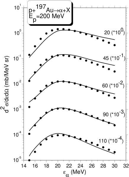
Figure 11: Fit with one source to the low energy data. The laboratory emission angle is given next to the appropriate data set or fit curve, respectively. The data and the fits were multiplied with the indicated factors.

Finally we report a fit value for the temperature of 3.12(17) MeV. There might be a correlation between the fit parameters. We have therefore performed moving source fits with barrier penetration to the angle integrated spectra, which will be discussed below. Unfortunately the different components are not clearly distinguishable as they are for the case of $\alpha$-particle emission from gold, thus resulting in fits which are not so good. But again we find rather small values for the barrier. It will be interesting to study further data around the barrier and to see whether the barrier is reduced in comparison to a nucleus in its ground state.

We use the slope and intercept parameters in Eq. (III) to get angle integrated cross sections. The angle integrated cross section is

$$\frac{d\sigma(\epsilon)}{d\epsilon}=\frac{2\pi}{a(\epsilon)}\left\{\exp\left[b(\epsilon)+a(\epsilon)\right]-\exp\left[b(\epsilon)-a(\epsilon)\right]\right\}.$$ (9)

The resulting differential cross sections for the three targets are shown in Figs 17–19. For the two lighter targets the energy distributions show an almost exponential slope without structure. In case of the gold target this structure is modified due to Coulomb effects. The distributions are discussed below.

IV Data Comparison

Although there are no data on IMF cross sections with exactly the same beam energy and for the same targets as employed in this study, there are data for energies or targets close by. We will compare the present data with those. First we will compare differential cross sections for the reaction $p+^{27}Al\to(A=7)+X$. For that purpose the present cross sections for ${}^{7}Li$ and ${}^{7}Be$ emission were added. In Fig. 12 these cross sections are compared with those from Kwiatkowski et al. Kwiatkowski83 taken at a beam energy of 180 MeV. They measured fragments with masses $A\geq 6$ and energies down to $\epsilon/A\geq 0.05$ MeV/$u$. The data have only a moderate overlap with the present data. There seems to be consistency between both data sets with respect to the absolute height as well as the shape of the spectra.

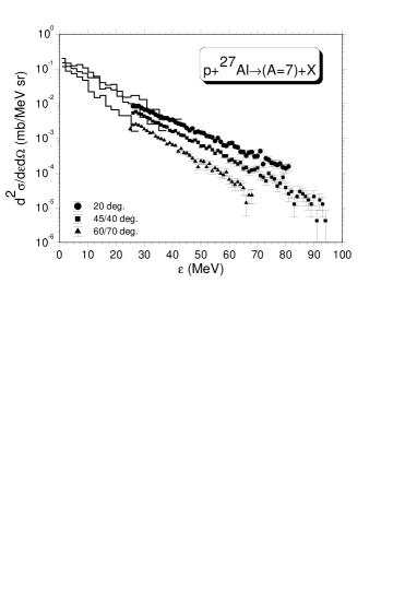
Figure 12: Double differential cross sections for $A=7$ emission following the bombardment of ${}^{27}Al$ with protons. The data from Ref. Kwiatkowski83 are shown as histograms and are for 180 MeV, the present data are shown as dots with error bars. The emission angles are given in the legend where the first angle is for the present data, the second for those from Ref. Kwiatkowski83 .

As already stated in the introduction there are two studies of IMF emission from $Ag$. One was performed at a proton beam energy of 161 MeV Yennello90 . Also these data cover smaller fragment energies than the present due to a gaseous $\Delta E$ detector. They observed fragments with charge number $Z$ ranging from 3 to 12.

Figure 13: Cross sections for total IMF production. The present data are shown by full symbols, those from Ref. Yennello90 by open dots and those by Ref. Green80 by open squares.

The total cross sections from this measurement are shown in Fig. 13 as function of the fragment charge number together with those from Green and Korteling Green80 and the present results. For the case of the aluminum targets a large fraction of the cross section is missing due to the thickness of the first $\Delta E$ detector used here (see the latter comparison with model calculations and Figs. 17-19). This makes the discrepancy in the yields esp. for $Z=5$ and 6. The yield in the case of the cobalt target agrees best in that of the silver target.

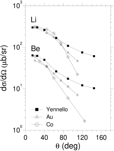
Figure 14: Angular distributions of $Li$ and $Be$ fragments for the indicated targets (this work) and for a silver target at 161 MeV proton energy Yennello90 .

In Fig. 14 angular distributions for $Li$ and $Be$ fragments integrated over the acceptance range are compared with those of Ref. Yennello90 . Again the agreement is reasonable with respect to the different energy ranges in the different experiments. Summarizing this comparison one can state that there is a fair agreement between the different measurements for $Z=3$ and 4. It may be more instructive to continue the comparison on the level of spectra.

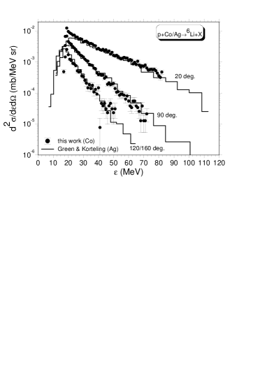
Figure 15: Comparison of double differential cross sections from the $p+^{59}Co\to^{6}Li+X$ reaction (this work, dots with error bars) and $p+Ag\to^{6}Li+X$ reaction (Ref. Green80 , histograms). The first angle given is for the present data while the second is for those from Green80 .

This is done in Fig. 15 for the case of isotopic ${}^{6}Li$ emission from $Ag$ (210 MeV, Ref. Green80 ) and ${}^{59}Co$. There is excellent agreement between the two data sets with respect to shape and absolute height. Finally we compare the slope of the present data in case of $\alpha$-particle emission for the aluminum and gold target with those of ref. Didelez82 . The later have been multiplied with an overall normalization factor of four. It becomes clear that the angular dependencies agree with each other in the overlap region.

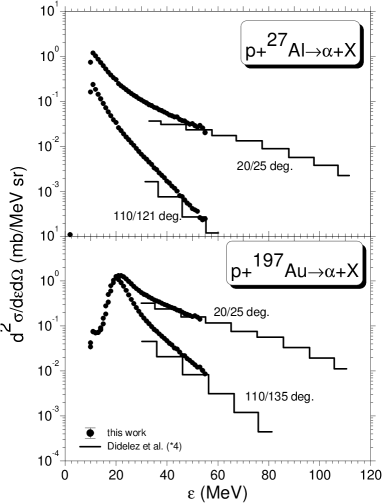
Figure 16: Similar as Fig. 15 but for the indicated reactions and data from Ref. Didelez82 , normalized by a factor of four.

From these comparison it becomes evident that one can state that the present data are correct with respect to spectral shapes, angular distributions and absolute magnitude of the cross sections.

V Comparison with model calculations

In this section model calculations are compared to the deduced data. A variety of models for fast particle emission in nuclear reactions are discussed in Ref. Machner85 . A model especially suited for higher projectile energies is the intranuclear cascade model (INC). Although it cannot account for IMFs during the equilibration process it predicts the final excitation energy of an equilibrated system. This system then undergoes de-excitation by evaporating lower energy particles.

The INC model was first proposed by Serber in 1947 Serber47 . The successful realization of this model by means of Monte Carlo simulations was published by Goldberger who did the first calculations by hand in 1948 Goldberger48 . Computer simulations were first done by Metropolis et al. Metropolis58 . In the present work we have applied the model in the standard Li$\grave{e}$ge version INCL4.2 Cugnon87 .

The Intranuclear Cascade (INC) Model simulates - by the Monte Carlo method - sequences of the nucleon-nucleon collisions proceeding inside the nucleus. This is equivalent to solving the Boltzmann transport equation for the time dependent distribution of the nucleons in the nucleus, treating explicitly collisions between the nucleons. As mentioned above, such a picture of the reaction is justified in the case when the energy of the projectile is high enough. The INC is stopped when signatures are fulfilled, which indicate equilibration of the decaying nucleus. In the INCL4.2 code the equilibration time $\tau$ is determined by reaching a constant emission rate of cascade particles during the INC process. Typically $\tau$ is of the order of $10^{-22}$s or 30 fm/c. The longer this somewhat “artificially” chosen time the smaller $E^{*}$ is left for the evaporation process. Here we have chosen

$$\tau=\tau_{0}\left(\frac{A_{T}}{208}\right)^{0.16}$$ (10)

with $\tau_{0}=44.1$ fm/c. This is smaller than the value used in Boudard02 but corresponds to the earlier used value Cugnon97 .

The description of each cascade involves three different stages: (i) initialization of the properties of the spatial and momentum distribution of nucleons in the nucleus, (ii) propagation of nucleons inside the nucleus, and (iii) collisions of the nucleons.

The simplicity of the model and speed of calculations makes the INCL model very attractive. Of course the model cannot efficiently describe evaporation of the particles from the compound nucleus formed in the first stage of the reaction for two reasons: (a) the evaporation is very sensitive to the density of states of the nuclei participating in the reaction, whereas the single particle density of states implicitly present in the INCL calculations is not exact enough, and (b) the calculations of the cascade over such long times as those characteristic for the compound nucleus emissions are not stable numerically and very inefficient. The other very serious drawback of the INCL model is absence of correlations between nucleons, which could lead to emission of complex fragments. This is because the INCL is a single particle model with the mean field treated in an oversimplified manner. The mean field used in the INCL makes the assumption of being constant throughout the volume of the nucleus or modified at the surface of the nucleus, but it is always a static field.

In practice the model of the intranuclear cascade (or equivalent) is applied to describe the first stage of the nuclear collision and the calculations are stopped once it can be assumed that equilibrium has been achieved. In the present study the INCL4.2 computer code was applied for this purpose. Discussion concerning the criteria for the terminating of the intranuclear cascade are presented by J. Cugnon et al. in Ref. Cugnon97 .

After equilibration is reached we apply an evaporation model. It is the generalized evaporation model (GEM) of Furihata Furihata00 , which is based on the classical Weisskopf – Ewing approach Weisskopf37 ; Weisskopf40 . According to this approach, the probability of evaporation of the particle $j$ from a parent compound nucleus $i$ with a total kinetic energy in the center-of-mass system between $\epsilon$ and $\epsilon$+d$\epsilon$ is defined as:

$$P_{j}(\epsilon)d\epsilon=g_{j}\sigma_{inv}(\epsilon)\frac{\rho_{d}(E-Q-\epsilon)}{\rho_{i}(E)}\epsilon d\epsilon,$$ (11)

where $E$ is the excitation energy of the parent nucleus $i$, $d$ denotes a daughter nucleus produced after the emission of ejectile $j$, and $\rho_{i}$, $\rho_{d}$ are the level densities for the parent and daughter nucleus respectively. $Q$ denotes the $Q$ – value of the reaction. The statistical and normalization factor $g_{j}$ is defined as $g_{j}=(2S_{j}+1)m_{j}/\pi^{2}\hbar^{2}$, where $S_{j}$ and $m_{j}$ are the spin and the mass of the emitted particle $j$ respectively. The cross section $\sigma_{inv}$ for the inverse reaction is evaluated from

$$\sigma_{inv}(\epsilon)=\sigma_{g}P(\epsilon))$$ (12)

where $\sigma_{g}$ is the geometrical cross section. GEM considers fragments heavier than helium nuclei. There are 66 ejectiles (see Table 1). For the barrier penetration probability $P$ we have used the form of Ref. Dostrovsky59 . The parameters for light particles (n, p, d, t, ³He and ⁴He) are taken from Ref. Dostrovsky59 whereas those for IMFs were adopted from the work of Matsuse et al. Matsuse82 .

Table 1: The ejectiles taken into consideration in the GEM calculations.

$Z_{j}$	Ejectiles
0	n
1	p	d	t
2	3He	4He	6He	8He
3	6Li	7Li	8Li	9Li
4	7Be	9Be	10Be	11Be	12Be
5	8B	10B	11B	12B	13B
6	10C	11C	12C	13C	14C	15C	16C
7	12N	13N	14N	15N	16N	17N
8	14O	15O	16O	17O	18O	19O	20O
9	17F	18F	19F	20F	21F
10	18Ne	19Ne	20Ne	21Ne	22Ne	23Ne	24Ne
11	21Na	22Na	23Na	24Na	25Na
12	22Mg	23Mg	24Mg	25Mg	26Mg	27Mg	28Mg

The total decay width $\Gamma_{j}$ is calculated by integrating Eq. (11) using Eq. (12) and is expressed as:

$$\Gamma_{j}=\frac{g_{j}\sigma_{g}}{\rho_{i}(E)}\int_{V}^{E-Q}\epsilon P(\epsilon)\rho_{d}(E-Q-\epsilon)d\epsilon.$$ (13)

where $V$ is the Coulomb barrier. For the level density we have applied the Fermi gas model expression

$$\rho(E) = \frac{\pi}{12}\frac{e^{2\sqrt{a(E-\delta)}}}{a^{1/4}(E-\delta)^{5/4}}\;\;\;\textrm{for}~{}E\geq E_{x}$$ (14)

$$= \frac{\pi}{12}\frac{1}{T}e^{(E-E_{o})/T}\;\;\;\;\;\;\;\;\;\textrm{for}~{}E\leq E_{x}$$ (15)

where $a=A_{d}/8$ (MeV^-1) is the level density parameter, $\delta$ is the pairing energy of the residual, $T$ is again the nuclear temperature given by $1/T=\sqrt{a/U_{x}}-1.5/U_{x}$ where $U_{x}$ is defined as $U_{x}=2.5+150/A_{d}$. The excitation energy E_x, for which the formula for level density changes its form, is evaluated as E_x=U_x+$\delta$. To obtain a smooth continuity between the two formulae, the E₀ parameter is determined as follows:

$$E_{0}=E_{x}-T\cdot(\ln T-0.25\ln a-1.25\ln U_{x}+2\sqrt{aU_{x}}).$$ (16)

The contribution of the emission of IMFs in a long living excited state is taken into account together with those which decay to the ground state. The condition for the lifetime of excited nuclei considered in GEM is as follows: $T_{1/2}/ln2>\hbar/\Gamma_{j}^{*}$. The value of $\Gamma_{j}^{*}$ is defined as the emission width of the decaying ejectile and is calculated in the same way as for the ground state, i.e. by Eq. (13). The total emission width of an ejectile is summed over its ground state and all its excited states. All input parameters are the standard parameters of the models. We have not adjusted parameters to fit the present data.

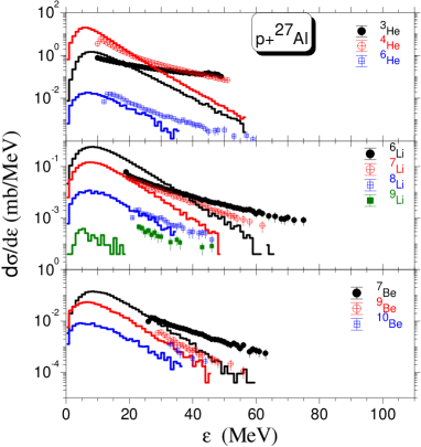
Figure 17: (Color online) Energy differential cross sections for indicated IMFs for aluminum. The data are shown by the different symbols indicated in the figure. The histograms are calculations described in the text.

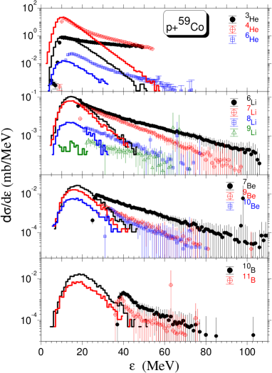
Figure 18: (Color online) Same as Fig. 17 but for cobalt.

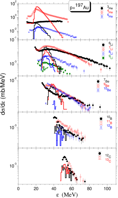
Figure 19: (Color online) Same as Fig. 17 but for gold.

In Figs 17–19 we compare the angle integrated cross sections with the results of the calculations sketched above. A general trend is visible. For high IMF energies the calculation underestimates the experiment. The non-equilibrium fraction of the cross section is quite large in agreement with other experiments Green80 ; Yennello90 . The heavier the IMFs are, the more the agreement between the calculations and data deteriorates, even in the evaporative region. Heavy IMFs are strongly underestimated. In the case of gold there is emission of IMFs from lighter composite systems, most probably fission fragments. This is also visible in the calculation but to a lesser extent than is observed in the data. The sequence within the isotopes is always obeyed by the calculations. However, in the case of ⁷Be emission from a gold-like composite the calculation predicts an almost negligible cross section, while the experiment is orders of magnitude higher. This is especially true for low energies and may point again to emission from lighter sources than the target-like system.

VI Discussion

We have measured IMF (He–C) emission for ²⁷Al, ⁵⁹Co and ¹⁹⁷Au targets at a proton beam energy of 200 MeV, which is near the maximal abundance in the proton distribution in cosmic rays. The fragments were isotopically resolved. Spectra were taken at laboratory angles from 20^oto 120^o. Analysis in terms of a model of a moving source with continuous temperature and source velocity shows a linear relationship between these two quantities as a function of particle energy. The data in the case of gold show a strong influence of the Coulomb barrier. In the cases of the two lighter targets this feature was suppressed by the thickness of the first $\Delta E$ counter. Emission of fragments with a significantly smaller Coulomb barrier than for a target-like system is observed. The assumption that we observe emission from excited fission fragments was studied in evaporation calculations. Indeed, the calculations also show such fragments (see $\alpha$-particle emission in Fig. 19), although with a cross section more than one order of magnitude smaller than the experiment. The data were compared to model calculations. The first stage was calculated with an intranuclear cascade. In this cascade the emission of pions and nucleons can take place. After equilibrium is reached the energy and momentum distribution of the excited composite is transferred to an evaporation model, which, in addition to nucleons, allows for IMF emission. The frequency of isotopes being emitted for a specific element is followed by the calculation. The high energy tails visible in the experiments are not reproduced by the calculations. The emission of the heavier isotopes like ⁹Li, ¹⁰Be, boron and carbon but also ⁷Be is underestimated.

The reduction of the Coulomb barrier observed may be due to dilution of the composite system. But an effect originating from the fission fragments can not be excluded. For the other two target nuclei we could not measure below the Coulomb barrier. Such data are highly desired to answer this question. Calculations, treating also IMF emission in the first fast stage are not yet available for the present data but are also desired.

Let us now come back to the problem of Galactic cosmic rays (GCR) as discussed in the introduction. The production of $BeB$ by Galactic cosmic-ray spallation of interstellar $CNO$ nuclei was the standard model for $BeB$ nucleosynthesis for almost two decades after first being proposed Reeves70 ; Meneguzzi71 . However, this simple model was challenged by the observations of $BeB$ abundances in Population II stars, and particularly the $BeB$ trends versus metallicity. Measurements showed that both $Be$ and $B$ vary roughly linearly with $Fe$, a ”primary” scaling. In contrast, standard GCR nucleosynthesis predicts that $BeB$ should be ”secondary” versus spallation targets $CNO$, giving $Be\propto O^{2}$ Vangioni-Flam90 . If $O$ and $Fe$ are coproduced (i.e., if the ratio $O/Fe$ is constant), then the data clearly contradict the canonical theory, i.e., $BeB$ production via standard GCR’s Fields00 . In order to accurately calculate the effects of the propagation of cosmic ray nuclei in the galaxy one needs to incorporate at least several hundred secondary cross sections into the propagation calculation. For charges with $Z<28$ this involves the fragmentation from $\approx 55$ nuclei with mass numbers A between 6 and 60 Webber98 . The present data should help to improve our understanding of the systematics of the cross sections as a function of Z, A, and A/Z.

In GCR’s one observes only stable isotopes since short lived isotopes decay. Thus only ${}^{3}He$ is observed because all tritium decays into it. The only difference might be ${}^{10}Be$ which has a half life of $1.6\times 10^{6}$ years. We therefore compare the ratio between ${}^{10}Be$ and ${}^{9}Be$ for the different targets. The yield of the short lived ${}^{9}Li$ is added to the latter. We report the ratio of the cross sections integrated over an energy range from 30 to 50 MeV in Table 2. Within this range for all three particle types data exist.

Table 2: The ratio $R=\sigma(^{10}Be)/[\sigma(^{9}Be)+\sigma(^{9}Li)]$ for the different targets in the energy range 30 to 50 MeV.

target	R
${}^{27}Al$	$0.654\pm 0.073$
${}^{59}Co$	$0.577\pm 0.133$
${}^{197}Au$	$0.918\pm 0.109$

The ratio in cases of the two lighter targets is within error bars identical. For gold the primordial abundance of ${}^{10}Be$ relative to the $A=9$ fragments is much larger than in the case of the two lighter targets. These ratios should be essential to study the age of GCR’s.

VII Acknowledgement

We acknowledge the cyclotron crew for providing us with the excellent beam. We thank C. J. Stevens (mechanics) and V. C. Wikner (electronics) for technical help in the preparation of the experiment.

References

- (1) P. Auger, R. Maze, P. Ehrenfest, A. Fréon: J. Phys. Radium, 10 (1939) 39.
- (2) R.H. Brown, et al.: Philos. Mag., 40 (1949) 862.
- (3) C.F. Powell, P.H. Fowler, D.H. Perkins: (1959) The Study of Elementary Particles by the Photographic Method, Pergamon Press, New York.
- (4) B. D. Fields, K. A. Olive, E. Vangioni-Flam, M. Cassé: Astrophysical Journal, 540 (2000) 930.
- (5) P. L. Biermann, N. Langer, Eun-Suk Seo, T. Stanev: Astronomy Astrophysics, 369 (2001) 269.
- (6) J. R. Hörandel, et al.: (2001) in Proceedings of 27th International Cosmic Ray Conference, Copernicus Gesellschaft (www.copernicus.org/C4/index.htm), page 1608.
- (7) G. A. de Nolfo et al.: (2001) in Proceedings of 27th International Cosmic Ray Conference, Copernicus Gesellschaft (www.copernicus.org/C4/index.htm), page 1667.
- (8) R. Michel, I. Leya, L. Borges: Nucl. Instruments and Meth. in Phys. Res., B 113 (1996) 343.
- (9) C.J. Waddington, J.R. Cummings, B.S. Nilsen, T.L. Garrard: Astr. Phys. J., 519 (1999) 214.
- (10) J. Hüfner: Phys. Rep., 125 (1985) 129.
- (11) R. Silberberg, C.H. Tsao: Phys. Rep., 191 (1990) 351.
- (12) S. Austin: Progress in Part. Nucl. Phys., 7 (1981) 1.
- (13) J. A. Simpson: Ann. Rev. Nucl. Part. Sci., 33 (1983) 323.
- (14) J. P. Didelez et al.: www.fz-juelich.de/ikp/gem under Conference Proceedings and Ricerca Scientifica ed Educazione Permanente, Suppl. 28 (1982) 237.
- (15) H. Machner et al.: Phys. Lett., B 138 (1984) 39.
- (16) C. Kalbach: Phys. Rev., C 37 (1988) 2350.
- (17) C. Kalbach: priv. communication to H. M.
- (18) R. E. L. Green, R. G. Korteling: Phys. Rev., C 22 (1980) 1594.
- (19) S. J. Yennello et al.: Phys. Rev., C 41 (1990) 79.
- (20) J. V. Pilcher, A. A. Cowley, D. M. Whittal, J. J. Lawrie: Phys. Rev., C 40 (1989) 1973.
- (21) W. Markiel et al.: Nucl. Phys., A 485 (1988) 445.
- (22) H. Machner: Z. Physik, A 336 (1990) 209.
- (23) C. Y. Wong: Phys. Lett., B 42 (1972) 156.
- (24) C. Y. Wong: Phys. Rev. Lett., 31 (1973) 77.
- (25) H. Machner: Phys. Rep., 127 (1985) 309.
- (26) V. E. Viola, T. Sikkeland: Phys. Rev., 128 (1962) 767.
- (27) H. Kwiatkowski et al.: Phys. Rev. Lett., 50 (1983) 1648.
- (28) R. Serber: Phys. Rev., 72 (1947) 1113.
- (29) M. Goldberger: Phys. Rev., 74 (1948) 1269.
- (30) N. Metropolis et al.: Phys. Rev., 110 (1958) 185.
- (31) J. Cugnon: Nucl. Phys., A 462 (1987) 751.
- (32) A. Boudard, J. Cugnon, S. Leray, C. Volant: Phys. Rev., C 66 (2002) 044615.
- (33) J. Cugnon, C. Volant, S. Vuillier: Nucl. Phys., A 620 (1997) 475.
- (34) S. Furihata: Nucl. Instruments and Meth. in Phys. Res., B 171 (2000) 251.
- (35) V. F. Weisskopf et al.: Phys. Rev., 52 (1937) 295.
- (36) V. F. Weisskopf, D. H. Ewing: Phys. Rev., 57 (1940) 472.
- (37) I. Dostrovsky et al.: Phys. Rev., 116 (1959) 683.
- (38) T. Matsuse, A. Arima, S.M. Lee: Phys. Rev., C 26 (1982) 2338.
- (39) H. Reeves, W. A. Fowler, F. Hoyle: Nature, 226 (1970) 727.
- (40) M. Meneguzzi, J. Audouze, H. Reeves: Astronomy Astrophysics, 15 (1971) 337.
- (41) E. Vangioni-Flam, M. Cassé, J. Audouze, Y. Oberto: Astrophysical Journal, 364 (1990) 568.
- (42) W. R. Webber et al.: Phys. Rev., C 58 (1998) 3539.