Proposal

for the

SPIN PHYSICS FROM COSY TO FAIR
A proposed programme for polarisation experiments in the COSY ring which could open the way to a polarised antiproton facility at FAIR

Jülich, August 2005

S. Barsov⁴, V.G. Baryshevsky⁵, M. Büscher², M. Capiluppi⁶, J. Carbonell⁷, G. Ciullo⁶, D. Chiladze², M. Contalbrigo⁶, P.F. Dalpiaz⁶, S. Dymov⁸, A. Dzyuba², R. Engels², P.D. Eversheim⁹, A. Garishvili¹⁰, A. Gasparyan¹¹, R. Gebel², V. Glagolev¹², K. Grigoriev⁴, A. Gussen¹¹, D. Gussev⁸, J. Haidenbauer², C. Hanhart², M. Hartmann², V. Hejny², P. Jansen¹³, I. Keshelashvili², V. Kleber², F. Klehr¹³, H. Kleines¹⁴, A. Khoukaz¹⁵, V. Koptev⁴, P. Kravtsov⁴, A. Lehrach², P. Lenisa⁶, V. Leontiev², B. Lorentz², V. Komarov⁸, A. Kulikov⁸, V. Kurbatov⁸, I. Lehmann¹⁶,G. Macharashvili⁸, Y. Maeda², S. Martin², T. Mersmann¹⁵, I. Meshkov⁸, M. Mielke¹⁵, M. Mikirtytchiants⁴, S. Mikirtytchiants⁴, U.-G. Meißner², S. Merzliakov⁸, A. Mussgiller², M. Nekipelov², N.N. Nikolaev², M. Nioradze¹⁰, D. Oellers², H. Ohm², Z. Oragvelidze¹⁰, M. Papenbrock¹⁵, D. Prasuhn², T. Rausmann¹⁵, M. Rentmeester¹⁷, J. Sarkadi², R. Schleichert², V. Serdjuk⁸, H. Seyfarth², A. Smirnov⁸, M. Stancari⁶, M. Statera⁶, E. Steffens¹, H. Ströher², A. Sydorin⁸, M. Tabidze¹⁰, P. Engblom-Thörngren¹⁶, S. Trusov⁸, Yu. Uzikov⁸, Yu. Valdau², A. Vassiliev⁴, M. Wang⁶, S. Yaschenko¹, and I. Zychor¹⁸

¹Physikalisches Institut II, Universität Erlangen–Nürnberg, 91058 Erlangen, Germany
²Institut für Kernphysik, Forschungszentrum Jülich, 52425 Jülich, Germany
³Physics and Astronomy Department, UCL, London WC1E 6BT, U.K.
⁴High Energy Physics Department, PNPI, 188350 Gatchina, Russia
⁵Research Institute for Nuclear Problems, Belarusian State University, Minsk 220050, Belarus
⁶University of Ferrara and INFN, 44100 Ferrara, Italy
⁷Laboratoire de Physique Subatomique et de Cosmologie, 38026 Grenoble Cedex, France
⁸Joint Institute for Nuclear Research, DLNP, 141980 Dubna, Russia
⁹Helmoltz Institut für Strahlen und Kernphysik, Universität Bonn, 53115 Bonn, Germany
¹⁰High Energy Physics Institute, Tbilisi State University, 0186 Tbilisi, Georgia
¹¹Institute for Theoretical and Experimental Physics, 117259 Moscow, Russia
¹²Joint Institute for Nuclear Research, VBLHE, 141980 Dubna, Russia
¹³Zentrallabor Technologie, Forschungszentrum Jülich, 52425 Jülich, Germany
¹⁴Zentrallabor Elektronik, Forschungszentrum Jülich, 52425 Jülich, Germany
¹⁵Institut für Kernphysik, Universität Münster, 48149 Münster, Germany
¹⁶Department of Radiation Sciences, Box 535, S–751 21, Uppsala, Sweden
¹⁷Institute for Theoretical Physics, Radboud University Nijmegen, Nijmegen, The Netherlands
¹⁸The Andrzej Soltan Institute for Nuclear Studies, 05400, Swierk, Poland

^a Email: a.kacharava@fz-juelich.de
^b Email: f.rathmann@fz-juelich.de
^c Email: cw@hep.ucl.ac.uk

1 Executive Summary

1.1 Introduction

It is the aim of the ANKE–COSY spin collaboration to carry out a well directed programme of internationally competitive experiments involving polarised beams and targets, using the outstanding facilities available at the storage ring. These activities, at the same time, are good preparation for our participation in the PAX@FAIR project. This Executive Summary will present a short description of the apparatus that can be used for this purpose at COSY and then discuss some of the principal experiments that will be undertaken within the scope of this collaboration. It concludes by outlining the PAX proposal.

1.2 Experimental Facilities

COSY accelerates and stores unpolarised and polarised protons and deuterons in a momentum range between 0.3 GeV/c and 3.7 GeV/c. To provide high quality beams, there is an Electron Cooler at injection and a Stochastic Cooling System from 1.5 GeV/c up to the maximum momentum. Transversally polarised beams of protons are available with intensities up to $1.2\times 10^{10}$ (with multiple injection and electron cooling and stacking) and polarisations of more than 80%. For deuterons an intensity of about $3\times 10^{10}$ was achieved in the February 2005 run with vector and tensor polarisations of more than 70% and 50% respectively.

Fast particles can be measured in the ANKE magnetic spectrometer installed at an internal beam position of COSY. Detection systems for both positively and negatively charged particles include plastic scintillator counters for TOF measurements, multi–wire proportional chambers for tracking, and range telescopes for particle identification. A combination of scintillation and Čerenkov counters, together with wire chambers, allow one to identify negatively charged pions and kaons. The forward detector, comprising scintillator hodoscopes, Čerenkov counters, and fast proportional chambers, is used to measure particles with high momenta, close to that of the circulating COSY beam. There is also a detector that can be used as a spectrometer for backward–emitted particles.

Although strip and cluster–jet targets have been standard for use at ANKE, we are currently in the process of installing a polarised internal target (PIT) system, consisting of an atomic beam source, feeding a storage cell, and a Lamb–shift polarimeter. The cell, which will increase tremendously the available luminosity, was tested in situ in February 2005 and the whole apparatus will be ready for commissioning experiments in early 2006. The design is such that the target and polarimeter can be moved in and out of the beam position, depending upon the requirements of the experiment.

One of the major advantages of doing experiments at a storage ring is that very low energy particles emanating from the very thin targets can be detected in silicon tracking telescopes placed in the target chamber. These are used to help in the measurement of elastic scattering, which is vital for luminosity and polarisation calibrations and, for a long target, establishing the vertex position. However, their most exciting use is for measuring the angles and energies of low energy protons ($<10$ MeV) that emerge as so–called spectators from the interactions of beam protons with the neutrons in the deuterium target. This information allows one to determine the proton–neutron centre–of–mass energy with high accuracy and will permit the study of a whole range of $pn$ elastic and inelastic reactions. The development of very thick (5–20 mm) double–sided micro–structured Si(Li) and very thin (69 $\mu$m) double–sided Si detectors provides a very flexible system for the use of the telescopes in particle identification and angle and energy measurement which, in the case of protons, will be from about 2.5 MeV up to 40 MeV. Each spectator detector can have typically a 10% geometrical acceptance with respect to a point target and, depending upon the needs of an individual experiment, up to four or six telescopes could be employed.

Although some information on the beam polarisation is available from the source, the standard methodology for determining it will be through the comparison with several reactions with known analysing powers that can be measured simultaneously in ANKE. For example, in the interaction of polarised deuterons with a hydrogen target, the vector and tensor polarisations could each be determined in three different ways at 1.17 GeV. At energies where the calibration reactions are unavailable, it is possible to use the polarisation export technique where, say, the deuteron beam polarisation is measured at 1.17 GeV, the energy is ramped to the region of interest for the physics measurement, before being reduced again to 1.17 GeV, where the beam polarisation is remeasured to check that any depolarisation is unimportant. We have shown that this method works very well for both proton and deuteron beams. The polarisation of the target cell will also be checked through known standards, some of which we ourselves will establish with the polarised beams.

1.3 Physics Programme

With the equipment available, many reactions will necessarily be detected simultaneously. However, in order to give a flavour of our rich programme, we here describe a few of the most important ones for which there is minimal ambiguity in the interpretation. A more complete compilation, listing our order of priorities, will be found in the main part of this document.

1.3.1 Proton–Neutron Spin Physics

The nucleon–nucleon interaction is fundamental to the whole of nuclear physics and hence to the composition of matter as we know it. Apart from its intrinsic importance, it is also a necessary ingredient in the description of meson production and other processes. The meticulous investigation of the nucleon–nucleon interaction must be a communal activity across laboratories, with no single facility providing the final breakthrough. However, the mass of EDDA data on $pp$ scattering has reduced significantly the ambiguities in the $I=1$ phase shifts up to 2.1 GeV. Nevertheless, the lack of good neutron–proton spin–dependent data make the $I=0$ phase shifts very uncertain above 800 MeV and there are even major holes in the knowledge between 515 and 800 MeV. We propose to add significantly to the elastic scattering data set by making measurements of cross sections, analysing powers, and spin–correlation coefficients near both the forward and backward directions by using the deuteron as a source of quasi–free neutrons. This substitute target has been shown at other laboratories to work well, though theoretical input is necessary to extract the $pn$ amplitudes reliably, especially at small momentum transfers.

Small angle neutron–proton scattering, which is difficult to study with a neutron beam, will be investigated up to 1.1 GeV per nucleon using the beam of polarised deuterons interacting in the polarised hydrogen target. One fast spectator proton will be detected in the ANKE magnetic system and the struck proton in the silicon telescopes. This is possible in an interval dictated by the telescope system, corresponding to momentum transfers $0.005<|t|<0.1$ GeV/c².

By using a deuterium target and detecting now the slow spectator proton in the telescopes, the beam energy range could be extended up to $\approx 3$ GeV though, to connect with the $pp$ phase shifts, the range up to 2.1 GeV is the most important. In this configuration the kinematic interval is fixed mainly by the measurement of the fast proton in ANKE ($4^{\circ}<\theta_{p}^{lab}<11^{\circ}$). Though in both configurations there are deuteron effects that suppress certain amplitudes, the necessary corrections can be largely handled, and the measurement of the slow proton leads to a good vertex identification even in the long target provided by the target cell. Since the projected counting rates are very high, it will be reasonable to take data in 100 MeV steps.

It has already been shown that ANKE is an efficient tool for measuring small angle charge exchange of polarised deuterons, $\vec{d}p\to(pp)n$, where the final $pp$ pair is at such low excitation ($<3$ MeV) that it is almost exclusively in an $S$ state. In this case the reaction provides a spin filter that selects an $np$ charge–exchange spin–flip from the (${}^{3}\!S_{1}$, ${}^{3}\!D_{1}$) states of the deuteron to the ${}^{1}\!S_{0}$ of the diproton. Measurements of the deuteron tensor analysing powers then allow one to extract the magnitudes of the different spin–spin $np\to pn$ amplitudes in the backward direction. The same type of experiments carried out with a polarised target determines the relative phases of these amplitudes. Though the selectivity of the ${}^{1}\!S_{0}$ region is clear, experience at Saclay shows that valuable information on the charge–exchange amplitudes is contained also in the higher $pp$ excitation data.

We have already shown in practice that the charge–exchange reaction can also be carried out in inverse kinematics, with both protons from a deuterium target being detected in the spectator counters. This would allow the energies up to 3 GeV to be used, though over a rather smaller momentum–transfer interval.

It is important to stress that, with the apparatus available, the studies of the small and large angle elastic neutron–proton scattering will be carried out simultaneously at ANKE.

1.3.2 Deriving the chiral three–body force from pion production

Chiral perturbation theory represents the best current hope for a reliable and quantitative description of hadronic reactions at low energies. One important step forward in our understanding of pion reactions at low energies will be to establish that the same short–range $NN\to NN\pi$ vertex contributes to both $p$–wave pion production and to low energy three–nucleon scattering, where the identical operator plays a crucial role. In the chiral Lagrangian, at leading and next–to–leading order, all but one term can be fixed from pion–nucleon scattering. The missing term corresponds to an effective $NN\to NN\pi$ vertex, where the pion is in a $p$–wave and both initial and final $NN$ pairs are in relative $S$ waves.

To second order in the pion momentum, nine observables are required to perform the full amplitude analysis in order to extract in a model–independent way the effective coupling constant. Of these, data from TRIUMF and CELSIUS yield seven at a beam energy around 350 MeV. Experiments designed to provide the necessary overconstraints will be carried out at ANKE through measurements of the analysing powers and spin–correlation parameters in the reactions $pp\to pp\pi^{0}$ and $pn\to pp\pi^{-}$.

It should be noted that the diproton detection in ANKE to isolate the ${}^{1}\!S_{0}$ state is just the same as that needed also for the $dp$ charge–exchange programme described earlier. The resolution on the $pp$ excitation energy is estimated to be around $0.3$ MeV and that on the missing mass about 5.5 MeV (RMS) which, at these low energies, will allow us to distinguish unambiguously the pion production reaction from any background. The counting rates are quite high and, even in the $pn\to pp\pi^{-}$ case, where the spectator proton has to be detected, more than $10^{3}$ events per hour could be accumulated over the full range of pion centre–of–mass angles.

Our facility offers the exciting possibility of extracting pion–production amplitudes in a model independent way and thus determining a vital parameter for chiral perturbation theory.

1.3.3 Strangeness production: The $\Lambda$–$N$ scattering length

Effective field theories provide the bridge between the hadronic world and QCD. For systems with strangeness, there are still many open questions and it is not even clear if the kaon is more appropriately treated as heavy or light particle. To improve further our understanding of the dynamics of systems containing strangeness, better data are needed. The insights to be gained are relevant, not only for few–body physics, but also for the formation of hypernuclei, and might even be of significance for the structure of neutron stars. The hyperon–nucleon scattering lengths are obvious quantities of interest in this context.

The IKP theory group has developed a method to enable one to deduce a scattering length directly from data on a production reaction, such as $pp\to pK^{+}\Lambda$, in terms of an integral over the invariant $\Lambda p$ mass ($m_{X}$) distribution. Using this method it can be seen that the inclusive Saclay $pp\to K^{+}X$ data, which had a mass resolution of 4 MeV, allow the extraction of a scattering length with an experimental uncertainty of only 0.2 fm. However, the actual value of the scattering length obtained in this way is not meaningful, since it represents the incoherent sum of the ${}^{3}\!S_{1}$ and the ${}^{1}\!S_{0}$ $\Lambda p$ final states with unknown relative weights. It is important to try to separate them.

The $\Lambda N$ triplet final state could be isolated unambiguously by measuring the unpolarised $K^{+}$ spectrum in the forward direction and this weighted with the incident spin correlation, obtained using a transversally polarised beam and target. This will be achieved by using the $\vec{p}\,\vec{d}\to p_{sp}K^{+}X$ reaction, since the spectator proton ($p_{sp}$) will provide a better determination of the vertex in the long polarised target cell.

In fact, by measuring the $K^{+}$ production rates in the near–threshold region in hydrogen and deuterium, and the spin–correlation in the deuterium case, we will also determine in a model–independent way the magnitudes of the three $S$–wave spin–isospin amplitudes, two corresponding to the spin–triplet final state and one to the singlet. It is also possible with a deuterium target to measure spin–transfer coefficients from the initial proton or neutron to the final $\Lambda$, and these will fix the relative phases of the three amplitudes. A significant $m_{X}$ variation in the singlet–triplet interference would point at a strong spin dependence of the $\Lambda n$ final state interactions, though much more theoretical work would be required to extract quantitative differences in the scattering lengths from such data.

1.4 $\mathcal{P}AX$: Polarised Antiproton eXperiments at FAIR

The possibility of testing nucleon structure through double–spin asymmetries in polarised proton–antiproton reactions at the High Energy Storage Ring (HESR) at the future Facility for Antiproton and Ion Research (FAIR) at GSI was suggested by the PAX collaboration in 2004. Since then, there has been much progress, both in understanding the physics potential of such an experiment and in studying the feasibility of efficiently producing polarised antiprotons. The physics programme of such a facility would extend to a new domain the exceptionally fruitful studies of the nucleon structure performed in unpolarised and polarised deep inelastic scattering (DIS), which have been at the centre of high energy physics during the past four decades.

A viable practical scheme using a dedicated low–energy antiproton polariser ring (APR) has been developed and published, which allows a polarisation of the stored antiprotons at HESR–FAIR of $\simeq 0.3$ to be reached. The approach is based on solid QED calculations of the spin transfer from electrons to antiprotons, which were confirmed experimentally in the FILTEX experiment. The method is routinely used at J–Lab for the electromagnetic form factor separation.

The polarised antiproton–proton interactions at HESR will provide unique access to a number of new fundamental physics observables, which cannot be studied without transverse polarisation of protons and antiprotons.

The transversity distribution is the last missing leading–twist piece of the QCD description of the partonic structure of the nucleon. It describes the quark transverse polarisation inside a transversely polarised proton. Unlike the more conventional unpolarised quark distribution $q(x,Q^{2})$ and the helicity distribution $\Delta q(x,Q^{2})$, the transversity $h^{q}_{1}(x,Q^{2})$ can neither be accessed in inclusive deep–inelastic scattering of leptons off nucleons nor can it be reconstructed from the knowledge of $q(x,Q^{2})$ and $\Delta q(x,Q^{2})$. It may contribute to some single–spin observables, but always coupled to other unknown functions. The transversity distribution is directly accessible uniquely via the double transverse spin asymmetry $\bf A_{TT}$ in the Drell–Yan production of lepton pairs, which is expected to be in the range 0.3–0.4. With the expected beam polarisation from the APR and the luminosity of HESR, the PAX experiment would make a definitive observation of $h^{q}_{1}(x,Q^{2})$ of the proton for the valence quarks. The determination of $h^{q}_{1}(x,Q^{2})$ will open new pathways to the QCD interpretation of single–spin asymmetry (SSA) measurements. In conjunction with the data on SSA from the HERMES collaboration, the PAX measurements of the SSA in Drell–Yan production on polarised protons would for the first time provide a test of the theoretical prediction of the reversal of the sign of the Sivers function from semi–inclusive DIS to Drell–Yan production.

The origin of the unexpected $Q^{2}$–dependence of the ratio of the magnetic and electric form factors of the proton, as observed at J–Lab, could be clarified by a study of their relative phase in the time–like region. This can be measured via SSA in the annihilation $\bar{p}p^{\uparrow}\to e^{+}e^{-}$ on a transversely polarised target. The first ever measurement of this phase at PAX would also contribute to the understanding of the onset of the pQCD asymptotics in the time–like region and would serve as a stringent test of dispersion theory approaches to the relationship between the space–like and time–like form factors. The double–spin asymmetry would allow an independent $G_{E}-G_{M}$ separation and serve as a check of the Rosenbluth separation in the time–like region.

Arguably, in $p\bar{p}$ elastic scattering the hard scattering mechanism can be checked beyond the $|t|=\frac{1}{2}(s-4m_{p}^{2})$ accessible in the crossed–symmetric $pp$ scattering, because in the $p\bar{p}$ case the $u$–channel exchange contribution can only originate from the strongly suppressed exotic dibaryon exchange. Consequently, in the $p\bar{p}$ case the hard mechanisms can be tested to transfers almost twice as large as in $pp$ scattering. Even unpolarised large angle $p\bar{p}$ scattering data can shed light on the origin of the intriguing oscillations around the $s^{-10}$ behavior of the $90^{\circ}$ scattering cross section in the $pp$ channel and put stringent constraints on the much disputed odd–charge conjugation Landshoff mechanism.

The PAX collaboration proposes an approach in two phases, with the eventual goal of an asymmetric proton–antiproton collider in which polarised protons with momenta of about 3.5 GeV/c collide with polarised antiprotons with momenta up to 15 GeV/c. These circulate in the HESR, which has already been approved and will serve the PANDA experiment. The overall machine setup of the HESR complex would consist of:

1. An Antiproton Polariser (APR) built inside the HESR area with the crucial task of polarising antiprotons at kinetic energies around $\approx 50$ MeV ($p\approx 300$ MeV/c), to be accelerated and injected into the other rings.

2. A second Cooler Synchrotron Ring (CSR, COSY–like) in which protons or antiprotons could be stored with momenta up to 3.5 GeV/c. This ring should have a straight section, where a PAX detector could be installed, running parallel to the experimental straight section of HESR.

3. By deflecting the HESR antiproton beam into the straight section of the CSR, both collider and fixed–target modes become feasible.

In Phase I a beam of unpolarised or polarised antiprotons with momenta up to 3.5 GeV/c in the CSR, will collide with a polarised hydrogen target in the PAX detector. This phase, which is independent of the HESR performance, will allow the first measurement of the time–like proton form factors in single and double polarised $\bar{p}p$ interactions over a wide kinematical range, from close to threshold up to $Q^{2}=8.5$ GeV². Several double–spin asymmetries in elastic $\bar{p}^{\uparrow}p^{\uparrow}$ scattering could be determined. By detecting back–scattered antiprotons one could also explore hard scattering regions of large $t$.

Phase II will allow the first ever direct measurement of the quark transversity distribution $h_{1}$, by studying the double transverse spin asymmetry $A_{TT}$ in the Drell–Yan processes $p^{\uparrow}\bar{p}^{\uparrow}\rightarrow e^{+}e^{-}X$ as a function of Bjorken $x$ and $Q^{2}$ (= $M^{2}$)

$$\mbox{$A_{TT}$}\equiv\frac{d\sigma^{\uparrow\uparrow}-d\sigma^{\uparrow\downarrow}}{d\sigma^{\uparrow\uparrow}+d\sigma^{\uparrow\downarrow}}\,=\,\hat{a}_{TT}\frac{\sum_{q}e_{q}^{2}h_{1}^{q}(x_{1},M^{2})h_{1}^{\overline{q}}(x_{2},M^{2})}{\sum_{q}e_{q}^{2}q(x_{1},M^{2})\overline{q}(x_{2},M^{2})}\,,$$

where $q=u,d,\ldots$, $\overline{q}=\overline{u},\overline{d}\ldots$, and $M$ is the invariant mass of the lepton pair. The parameter $\hat{a}_{TT}$, which is of the order of one, is the calculable double–spin asymmetry of the elementary QED process $q\overline{q}\rightarrow e^{+}e^{-}$.

Two possible scenarios, an asymmetric collider or a high luminosity fixed target experiment, might be foreseen to perform the measurement. A beam of polarised antiprotons from 1.5 GeV/c up to 15 GeV/c circulating in the HESR, collides with a beam of polarised protons with momenta up to 3.5 GeV/c circulating in the CSR. This scenario, however, requires one to demonstrate that a suitable luminosity is reachable. Deflection of the HESR beam to the PAX detector in the CSR is necessary. By a proper variation of the energy of the two colliding beams, this setup would allow a measurement of the transversity distribution $h_{1}$ in the valence region of $x>0.05$, with corresponding $Q^{2}=4\ldots 100$ $\rm GeV^{2}$. With a luminosity of $2\times 10^{30}$ cm^-2s^-1 about $1000$ events per day can be expected. Recent model calculations show that in the collider mode, luminosities in excess of $10^{30}$ cm^-2s${{}^{-}1}$ could be reached. For the transversity distribution $h_{1}$, such an experiment can be considered as the analogue of polarised DIS for the determination of the helicity structure function $g_{1}$, i.e. of the helicity distribution $\Delta q(x,Q^{2})$. The kinematical coverage in $(x,Q^{2})$ will be similar to that of the HERMES experiment.

If the required luminosity in the collider mode is not achievable, an experiment with a fixed polarised internal hydrogen target can be undertaken. In this case, an upgrading of the momentum of the polarised antiproton beam circulating in the HESR up to 22 GeV/c is envisaged. This scenario also requires the deflection of the HESR beam to the PAX detector in the CSR. This measurement will explore the valence region of $x>0.2$, with corresponding values of $Q^{2}=4\ldots 16$ GeV², yielding about 2000 events per day.

1.5 Conclusions

There are unique opportunities at ANKE to measure the spin dependence of many polarised reactions, primarily in the proton–neutron sector. This is through the combination of magnetic analysis of fast particles with the detection of slow particles in the silicon telescope array. The proton–neutron programme has already been started at ANKE by using polarised deuterons incident on an unpolarised target and the full programme with a polarised target will be initiated in 2006. In general the requisite equipment exists, or has already been financed, though minor upgrades may of course be necessary.

Many reactions will be measured simultaneously, but we will first concentrate on the nucleon–nucleon programme, where counting rates are high, before passing to the pion production and then to the more challenging of the strangeness experiments.

The experience that the team will gain in undertaking polarisation measurements will be put to good use in the developments for PAX at FAIR, to which the group as a whole is committed. The storage of polarised antiprotons at HESR, as proposed by PAX, will open unique possibilities to test QCD in hitherto unexplored regions, thereby extending into a new domain the exceptionally fruitful studies of nucleon structure performed in unpolarised and polarised deep inelastic scattering. This will provide another cornerstone to the contemporary QCD physics programme with antiprotons at FAIR.

Contents

1. 1 Executive Summary
   1. 1.1 Introduction
   2. 1.2 Experimental Facilities
   3. 1.3 Physics Programme
      1. 1.3.1 Proton–Neutron Spin Physics
      2. 1.3.2 Deriving the chiral three–body force from pion production
      3. 1.3.3 Strangeness production: The $\Lambda$–$N$ scattering length
   4. 1.4 $\mathcal{P}AX$: Polarised Antiproton eXperiments at FAIR
   5. 1.5 Conclusions
2. 2 Introduction
3. 3 Experimental Facilities
   1. 3.1 Polarised beams at COSY
   2. 3.2 ANKE magnetic spectrometer
   3. 3.3 Silicon tracking telescopes for the detection of spectator protons
      1. 3.3.1 The design concept
      2. 3.3.2 The detector performance
      3. 3.3.3 The in-vacuum electronics
      4. 3.3.4 The read–out system
      5. 3.3.5 The target cell arrangement
   4. 3.4 Polarised internal target
      1. 3.4.1 Status of the PIT and LSP development
4. 4 Beam and Target Polarimetry
   1. 4.1 Deuteron beam polarimetry
   2. 4.2 Polarisation export technique
   3. 4.3 Target polarimetry
   4. 4.4 Luminosity determination
5. 5 Proton–Neutron Spin Physics
   1. 5.1 Proton–neutron small angle elastic scattering
   2. 5.2 Proton–neutron elastic charge exchange
      1. 5.2.1 Charge–exchange with a polarised deuteron beam
      2. 5.2.2 Polarimetry reactions
      3. 5.2.3 Charge–exchange with a polarised deuterium target
   3. 5.3 Proton–neutron inelastic charge exchange
   4. 5.4 Small angle $\vec{p}\,\vec{d}$ or $\vec{d}\,\vec{p}$ elastic scattering
6. 6 Proton–Deuteron Reactions at High Momentum Transfers
   1. 6.1 Large angle $\vec{p}\,\vec{d}$ or $\vec{d}\,\vec{p}$ elastic scattering
   2. 6.2 $\vec{p}\,\vec{d}\to(pp)\,n$ at large momentum transfers
7. 7 Non–strange Meson Production
   1. 7.1 Deriving the chiral three–body force from pion production
      1. 7.1.1 Motivation
      2. 7.1.2 Details
      3. 7.1.3 Experimental considerations
   2. 7.2 $\vec{n}\,\vec{p}\to d\,X$
      1. 7.2.1 $\vec{n}\,\vec{p}\to d\,\pi^{0}$
      2. 7.2.2 $\vec{n}\,\vec{p}\to d\,\pi\pi$
   3. 7.3 The production of heavier non–strange mesons in $NN$ collisions
      1. 7.3.1 Missing–mass experiments
      2. 7.3.2 Exclusive measurements
      3. 7.3.3 Polarisation measurements
   4. 7.4 Meson production in $\vec{p}\,\vec{d}\to\,^{3}\textrm{He}\,X$ reactions
      1. 7.4.1 $\vec{p}\,\vec{d}\to\,^{3}\textrm{He}\,\pi^{0}$
      2. 7.4.2 $\vec{p}\,\vec{d}\to\,^{3}\textrm{He}\,\eta$
      3. 7.4.3 $\vec{p}\,\vec{d}\to\,^{3}\textrm{He}\,ABC$
8. 8 Production of Strange Mesons and Baryons
   1. 8.1 Determination of the spin–triplet $\Lambda-N$ scattering length
   2. 8.2 The $NN\rightarrow NK\Lambda$ reaction near threshold
   3. 8.3 Experimental considerations
9. 9 Test of Time–Reversal Invariance in Proton–Deuteron Scattering
   1. 9.1 Overview
   2. 9.2 Introduction
   3. 9.3 Experimental set–up
   4. 9.4 First results
10. 10 Spin Rotation and Birefringence in Storage Rings
11. 11 Preparatory Work for the FAIR Project
    1. 11.1 The PAX proposal at FAIR
    2. 11.2 Preparatory phase
    3. 11.3 Spin Filtering Experiments with protons at COSY and with antiprotons at the CERN AD
    4. 11.4 Design and construction of the Antiproton Polariser Ring
    5. 11.5 Development of polarised sources
    6. 11.6 Staging of the PAX experiment and the role of COSY
    7. 11.7 Phase–I: transfer of APR and CSR to FAIR
    8. 11.8 Phase–II: HESR modifications to the collider mode or to the polarised internal target
12. 12 Time Schedules
    1. 12.1 General remarks
    2. 12.2 Submissions and requests
    3. 12.3 Timelines

2 Introduction

For several years COSY has provided circulating beams of polarised protons. Used together with a polarised hydrogen target, these beams have been successfully exploited by the EDDA collaboration to measure the cross section, the analysing power and spin–correlation observables in proton–proton elastic scattering over much of the COSY energy range [1]. Vector and tensor polarised deuteron beams are also available up to an energy of about $T_{d}\approx 2.3$ GeV. Using such capabilities to the full is one of the stated priorities of the laboratory: For spin–physics experiments, the FZJ proposes to increase the intensity of the polarized beams up to the space charge limit [2].

In 2005, a polarised internal hydrogen and deuterium storage–cell target (PIT) has been installed at the ANKE spectrometer. A Lamb–shift polarimeter (LSP) will allow the adjustment of the transition units of the polarised atomic beam source (ABS) that feeds the storage cell. Thus it is expected that late in 2006 the whole system of polarised beam and polarised target will be fully operational inside the COSY ring at the ANKE position, where fast charged particles can be magnetically analysed and slow particles measured using telescopes of silicon counters placed around the target. We will therefore soon be in a position to carry out many of the recommendations of the 1998 workshop on Intermediate Energy Spin Physics [3].

Under these circumstances it is incumbent on us to make a global presentation to the PAC of the spin programme that will exploit these advanced facilities over the years to come. We will be concerned only with experiments that could be carried out within the confines of the COSY storage ring by detecting charged particles. In this spirit, the investigation of charge–symmetry breaking in the polarised $\vec{d}\,d\to\alpha\,\pi^{0}$ reaction is described rather in the WASA proposal [4]. Furthermore, the relation to external experiments, such as TOF, must await the preparation of further plans by these collaborations. No requests are made here for beam time for particular experiments; these will only follow later in conjunction with more detailed and specific proposals.

However, this is also a period of transition for experimental hadronic physics in Germany, with the plans to construct the Facility for Antiproton and Ion Research (FAIR) at GSI Darmstadt [5]. Though the scale of this operation, involving the building of a high energy antiproton storage ring (HESR), is vastly bigger than that at COSY, there is a great potential synergy in respect of the spin physics programmes at the two laboratories and, for the future of the field, an orderly transfer of physics interest between the two is highly desirable. Target development, polarimetry, cooled beams, spectator proton detection etc. are all areas that are covered in the technical aspects of §11 in the context of an eventual knowledge transfer to FAIR.

It is expected that antiprotons can be polarised through the spin–transfer from the polarised electrons of the atoms in a polarised target to orbiting antiprotons [6, 7, 8, 9]. This could be carried out at FAIR in a separate antiproton polariser ring, using a polarised internal storage cell target [10]. A Letter–of–Intent, describing some of the important experiments that can be carried out with polarised beams and targets at FAIR, was submitted in February 2005 to the GSI QCD–PAC by the PAX collaboration [11]. This was well received by this committee and the relevant recommendations are [12]:
“The PAC considers it is essential for the FAIR project to commit to polarized antiproton capability at this time and include polarized transport and acceleration capability in the HESR, space for installation of the APR and CSR and associated hardware, and the APR in the core project. We request the PAX collaboration to:
1) Commit to the construction and testing of the APR (IKP Jülich appears to be the optimal location)
2) Explore all options to increase the luminosity to the target value specified above
3) Prepare a more detailed physics proposal and detector design for each of the proposed stages.”

Though the principles of the polarising technique have been well established for low energy protons [6, 7, 8], an investigation with medium energy protons should be undertaken at COSY. The lead–up to FAIR physics is discussed in §11. Before that, in §3, we describe in detail the technology that we will have at our disposal in terms of polarised beams/targets and detectors to carry out the COSY programme. It is clear that we must ourselves be able to measure the polarisation of the beams and/or targets and not rely exclusively on outside polarimetry. How this will be done is the subject of §4.

It is universally agreed that a detailed understanding of nucleon–nucleon scattering, at least at a phenomenological level, up to high energies is a “good thing”, and that this involves a systematic compilation of experiments at different laboratories. Though EDDA has clarified significantly the spin dependence of the proton–proton scattering amplitudes up to at least 2 GeV [1], the data base of spin–observables in neutron–proton scattering is very incomplete above 800 MeV, so that there are large uncertainties in the isoscalar phase shifts. Section 1.3.1 shows how many of these holes can be filled by internal COSY experiments using a polarised deuteron beam or deuterium target. In addition to elastic neutron–proton scattering, important data should be obtained on the excitation of the $\Delta(1232)$ isobar, either explicitly through a $\pi N$ final state, or indirectly through $d\,\pi^{0}$ production. The measurement of up to triple–spin observables will be achieved. It is, however, very important to stress that many of the experiments involve high counting rates and will be carried out simultaneously with others provided that the trigger conditions allow this.

COSY generally operates at energies above the pion–production threshold and in such a domain the Faddeev equations are no longer able to describe proton–deuteron elastic scattering in a quantitative way, especially at large angles. This is due, in part, to the virtual excitation and de-excitation of the $\Delta(1232)$ isobar, which can help to share the large momentum transfer between the two nucleons in the deuteron. Although reactions such as this, or the analogous backward proton–deuteron charge exchange cannot, at present, be interpreted in an unambiguous way, it is hoped that spin observables will provide extra clues on the underlying dynamics. The possibilities here will be surveyed in §6.

The spin–dependence of the production of non–strange mesons in polarised nucleon–nucleon collisions is the subject of §7. It is shown that, even far from threshold, production of neutral mesons $X^{0}=\pi^{0},\,\eta,\,\omega,\,\dots$ through the $\vec{p}\,\vec{p}\to ppX^{0}$ reaction, with the two final protons at low excitation energy, contains valuable new information because of the spin–filter effect resulting from the two protons being in the ${}^{1}S_{0}$ state. Of especial interest is the production on neutrons via $\vec{p}\,\vec{n}\to pp\pi^{-}$ which, at low energies, could be a valuable check on effective field theory in the large momentum transfer regime. Also in this section we discuss what one can learn from coherent single and double pion production with the formation of a deuteron or ³He nucleus.

Two of the prime considerations in the construction of ANKE were the possibility of installing a polarised target and the ability to detect positive kaons against a high background of other particles. §8 shows that these two characteristics can be combined in a unique way to advance studies of $K^{+}\Lambda$ production in nucleon–nucleon collisions. Near threshold, the cross sections on protons and neutrons as well as the spin–correlation and –transfer parameters can all be efficiently measured and this allows one to isolate the spin–singlet and triplet $\Lambda N$ final states in a model–independent way. Some of these opportunities persist in the forward direction at higher energies and open the door to a quantitative investigation of the $\Lambda N$ scattering lengths in well–defined spin states.

Having stressed some of the strengths of ANKE that we shall exploit, we must also recognise its limitations. For example, the restricted phase space offered for exclusive reactions will not allow a meaningful exploration of the spin dependence of rare reactions, such as the production of the hypothesised exotic $\Theta^{+}(1540)$ baryon. With its much larger acceptance, such systematic studies might be better carried out at the TOF detector, where evidence for the existence of the state has already been presented [13].

The ambitious programme outlined in the following pages will take of the order of four years to complete and a series of milestones is suggested in the timetable presented in §12. There are, of course, many outstanding questions that cannot be answered at the present time. Is it feasible to construct a partial Siberian snake in COSY to rotate the polarisation axis of the beam using, in part, the WASA solenoid [4]? Will it be feasible to rotate the polarisation of the target? Finally, the future relationship of COSY with FAIR is also uncertain, and this bears directly on the importance of much of the work described here.

3 Experimental Facilities

3.1 Polarised beams at COSY

The COoler SYnchrotron COSY [14] accelerates and stores unpolarised and polarised protons and deuterons in a momentum range between 0.3 GeV/c and 3.7 GeV/c. To provide high quality beams, there is an Electron Cooler at injection and a Stochastic Cooling System from 1.5 GeV/c up to the maximum momentum. Vertically polarised proton beams of different momenta, with polarisations of more than 80%, are delivered to internal and external experimental areas. An rf dipole has been installed to induce artificial depolarising resonances.

Deuteron beams with different combinations of vector and tensor polarisation became available in 2003. The first simultaneous measurement of vector and tensor polarisation of the stored deuteron beam using the ANKE spectrometer is described in §4.1. The achieved intensities for polarised proton beams are $5\times 10^{9}$ (single injection with electron cooling) and $1.2\times 10^{10}$ with multiple injection with electron cooling and stacking. For the polarised deuterons with single injection an intensity of about $3\times 10^{10}$ was achieved during the February 2005 runs.

Increasing the phase space density by electron cooling at injection and conserving the beam emittance during internal experiments at high momenta through stochastic cooling are the two of the outstanding characteristics of COSY.

3.2 ANKE magnetic spectrometer

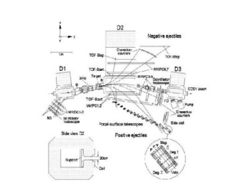
Figure 1: Schematic drawing of ANKE Spectrometer. Typical trajectories of ejectilies are indicated with emission angle of $0^{\circ}$ or $\pm 10^{\circ}$.

It is proposed that the experimental programme outlined in this document will be performed using the ANKE spectrometer, which is described in detail in ref [15]. The layout of this facility, which is installed at an internal beam position of COSY, is shown in Fig. 1. The main components of the spectrometer are: a magnetic system, an internal target and four detection systems — positive and negative side detectors, forward and backward detectors. The ANKE magnetic system comprises a dipole magnet D1, which deflects the circulating COSY beam through an angle $\alpha$, a large spectrometer dipole magnet D2 to perform the momentum analysis (beam deflection $-2\alpha$), and a third dipole magnet D3, identical to D1, to deflect the beam through $\alpha$ back to the nominal orbit.

Strip and cluster–jet targets have been used for many years at ANKE. The Polarised Internal Target (PIT), which was installed for tests at the ANKE position in July 2005, will be described in §3.4.

Detection systems for both positively and negatively charged particles include plastic scintillator counters for TOF measurements, multi–wire proportional chambers (MWPC) for tracking, and range telescopes for particle identification. A combination of scintillation and Čerenkov counters, together with wire chambers, allow one to identify negatively charged pions and kaons. The forward detector (FD), comprising scintillator hodoscopes, Čerenkov counters, and fast proportional chambers, is used to measure particles with high–momenta, close to that of the circulating COSY beam. A backward detector (BD), composed of hodoscopes and multi–wire drift chambers, together with the D1 magnet, can be used as a spectrometer for backward–emitted particles.

The silicon strip counters that are placed close to the target for vertex reconstruction and detection of low–energy spectator protons will be discussed separately in §3.3.

3.3 Silicon tracking telescopes for the detection of spectator protons

Modular Silicon Tracking Telescopes have been developed based on double–sided silicon strip detectors [16]. Serving in general for

• low energy spectator proton detection/tracking and

• vertex reconstruction into the ANKE target region,

they are optimised for the identification and measurement of low energy protons, determining their four–momenta. They allow one to use polarised deuterium gas as a polarised neutron target and to study e.g. reactions of the type $\vec{p}\,\vec{n}\rightarrow pnX$ or $\vec{p}\,\vec{n}\rightarrow dX$.

The telescopes are installed as close as 2 cm from the COSY beam inside the ultra high vacuum of the accelerator. Their basic features are $\Delta E/E$ proton–deuteron identification from 2.5 to 40 MeV and particle tracking over a wide dynamic range, either $2.5\,$MeV spectator protons or minimum–ionising particles. The recent development of very thick (5–20 mm) double–sided micro structured Si(Li) and very thin (69$\,\mu$m) double–sided Si–detectors provides the modular use of the telescopes for particle identification over a wide range of energies. Fig. 2 shows a telescope arrangement with a thin and a thick detector.

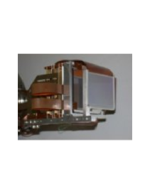
Figure 2: Telescope arrangement of double–sided silicon strip detectors: 69$\,\mu$m thin, $51\times 66\,$mm² active area as first layer and 5100$\,\mu$m thick, $64\times 64\,$mm² active area Si(Li) detector as second layer. Protons with kinetic energies in the range $2.5<T_{p}<35\,$MeV will be tracked and identified with such an arrangement.

3.3.1 The design concept

The basic design concept of a telescope is to combine particle identification and tracking over a wide energy range. The tracking of particles is accomplished through the use of double–sided silicon strip detectors. The minimum energy of a proton to be tracked is fixed by the thickness of the innermost layer. It will be detected when it passes through the inner layer and be stopped in the second. The maximum energy of protons that can be identified is given by the range within the telescope and therefore by the total thickness of all detection layers. Measuring the energy losses in the individual layers of the telescope permits the identification of stopped particles by the $\Delta E/E$ method. Hence by tracking and subsequently measuring precisely their energy, the telescopes determine the four–momenta for stopping particles.

To measure the momentum of a particle from the track information in the ANKE detection systems, the vertex of the reaction must be known and this is a non-trivial task for an extended storage cell target of up to 40 cm length. Only by having additional track(s) in the Silicon Tracking Telescopes close to the ANKE target region inside the COSY vacuum, can the vertex be reconstructed accurately.

Depending upon the requirements of the individual experiment, four to six telescopes can be equipped with different sets of silicon detectors and be positioned around the target region to serve for several purposes:

• Spectator Detector: Low energy protons will be identified and tracked in the range $2.5<T_{p}<35\,$MeV. Each telescope covers about 10% of the geometrical acceptance.

• Vertex Detector: One track in the Silicon Tracking Telescopes defines the vertex in two coordinates (along and perpendicular to the beam) with a precision of about 1 mm. The third coordinate can only be fixed using the spatial resolution of the ANKE detection system, which gives about 10 mm. Only two tracks from the same reaction inside the telescopes allows a full 3–D vertex reconstruction with a precision to about 1 mm. In such a case reactions on the walls of the storage cell can be easily identified.

• Polarimeter: Two protons in the telescopes from the $pp$ elastic or quasi–elastic scattering allows one to analyse the polarisation along the storage cell in parallel with the main experiment.

3.3.2 The detector performance

Two telescopes have been assembled to check the performance of the chosen detectors. For this purpose three types of double–sided position sensitive detectors are arranged as silicon tracking–telescopes.

• The inner layer is 69$\,\mu$m thick, has an active area of $51\times 66\,$mm², and an effective pitch of about $400\,\mu$m. Its thickness sets the detection threshold for protons in coincidence with the second layer at about 2.5 MeV.

• The second layer consists of a 300(500)$\,\mu$m thick detector with an active area of $51\times 66\,$mm² and a pitch of $\approx 400\,\mu$m. It stops protons of kinetic energies up to 6.3(8) MeV.

• The last layer is a 5500(10000)$\,\mu$m thick double–sided Si(Li) detector with a pitch of 666$\,\mu$m and an active area of $64\times 64$mm² [17]. It stops protons with energies up to 40 MeV and therefore covers most of the dynamic range of the telescope.

The recent development of very thick ($>10\,$mm) double–sided micro structured Si(Li) [17] and very thin (69$\,\mu$m) double–sided Si–detectors enables the use of the telescopes over a wide range of particle energies.

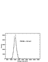
Figure 3: The energy loss in a 60$\,\mu$m vs that in a 300$\,\mu$m thick detector. Deuterons are not seen here because the detectors were placed in the backward hemisphere of the target. The right figure shows the energy resolution along the indicated slice perpendicular to the proton band.

The $\Delta E$/E performance of the detection system is demonstrated in Figs. 3 and 4. In addition to the experimental data the SRIM estimations [18] for the energy losses of protons and deuterons are drawn. With a careful calibration of the system they coincide to about $<3\,$%.

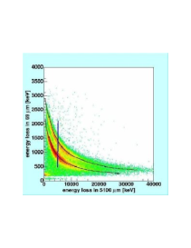
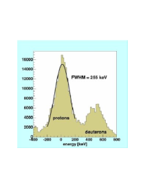
Figure 4: The energy loss in a 69$\,\mu$m vs that in a 5100$\,\mu$m thick detector. The right figure shows the energy resolution along the indicated slice perpendicular to the proton band.

The layout of these modular, self–triggering silicon tracking telescopes provides

• $\Delta$E/E proton identification from 2.5 up to 40(50) MeV with an energy resolution of 150–250 keV (FWHM). The telescope structure of 69/300/500/5000$\,\mu$m thick double–sided Si–strip detectors, read out by high dynamic range chips [19], allows $\Delta$E/E particle identification over this wide dynamic range.

• Particle tracking over a wide range of energies, either 2.5 MeV spectator protons or minimum–ionising particles. The angular resolution varies from 1^∘–6^∘ (FWHM). It is on the one hand limited by the angular straggling within the detectors and is therefore influenced by the track inclination. On the other hand (e.g. for minimum–ionising particles) it is limited by the strip pitch of about 400–700$\,\mu$m and the distances between the detectors. A typical vertex resolution for two low energy protons in the telescopes is on the order of $\approx 1\,$mm.

• Self–triggering capabilities. The telescopes identify a particle passage within 100 ns and provides the possibility to set fast timing coincidences with other detector components of the ANKE spectrometer.

• High rate capability. This becomes especially important for the polarimetry studies because, for this application, two telescopes have to be placed in the forward hemisphere. The fast–timing option of the amplifier chips allows one to suppress significantly accidentals.

3.3.3 The in-vacuum electronics

To combine a high dynamic range for the energy measurements with the requirement of self–triggering electronics the VA32TA2 chip has been developed [19]. The VA32TA2 houses 32 preamplifiers and 32 slow shaper amplifiers together with 32 corresponding fast shaper amplifiers and discriminators to get fast timing and trigger signals. The slow shapers provide charge integration with a peaking time of 2$\,\mu$s. The peak amplitude is sampled by applying a hold signal, supplied externally with the appropriate timing. The read–out is done over an up to 10 MHz multiplexed analogue output.

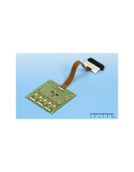
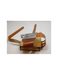
Figure 5: The left photo shows the chip board (here a G10 prototype) with 5 chips. Three input connectors couple it to one side of a detector, whereas one output connector interfaces to the vacuum feed–through. The right photo shows the assembly of one 300$\,\mu$m detector with its two ceramic boards.

The in–vacuum assembly of the chips is based on the use of $90\times 90\,$mm² double–sided Al₂O₃ ceramic boards (Fig. 5, left). Five chips are glued and bonded onto one ceramic board. This correspond to a maximum number of 160 read–out channels where 151 are actually fed to the connectors. Two of these boards serve to read out the front and backside of a double–sided detector (Fig. 5, right).

3.3.4 The read–out system

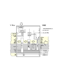
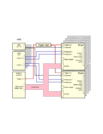
Figure 6: Left: The RCard block scheme. The Y–Flex part coming from the detector is electrically fully decoupled from the VME control part. Right: The block diagram of the VME read–out scheme. Two RCards are foreseen to read one double–sided silicon strip detector.

Fig. 6 shows the block scheme of the interface electronics between VME and the in–vacuum ceramic boards, the so–called RCard. Its main purpose is to decouple all bias and control lines of the chips on the ceramics that are operated at detector biases up to 1.5 kV. One card is needed for each side of a detector.

On the VME side the board provides a flat cable connector for all digital control signals of the board and the front–end electronics. Up to 16 RCards can be connected and addressed on a single common bus. All necessary control signals to read out the amplifier chips and to set the trigger pattern of the addressed RCard are provided over this flat–cable connection. Since the timing of the hold–signal for one VA32TA2 read–out chain is crucial for good performance, an adjustable delay is provided for this signal on each RCard. Two voltage inputs are provided which allow one to control the discriminator thresholds and the calibration pulse amplitude. The block scheme of the complete setup with all VME components is shown in Fig. 6 (right).

External 16-bit DACs are used for the generation of the VA32TA2 trigger thresholds on the RCards; Each threshold can be controlled individually. The ADCs have 10 bit resolution and are especially designed for the read–out of multiplexed analogue signals from silicon–strip detectors.

3.3.5 The target cell arrangement

The telescope systems are very flexible and their arrangement will depend upon the particular requirements of the experiment being carried out. For a point target one will generally try to cover a large part of the solid angle whereas for a target cell, one needs to cover its length, as illustrated in Fig. 7.

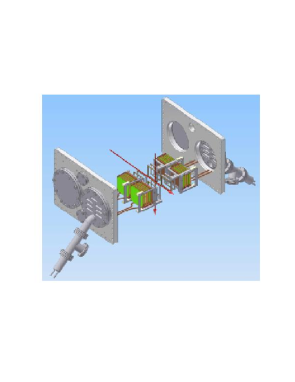
Figure 7: One of the possible arrangements with telescopes being placed side–by–side to cover a longer target cell.

3.4 Polarised internal target

The polarised internal target system consists of an atomic beam source feeding a storage cell and a Lamb–shift polarimeter. The status of the different components is here discussed.

The polarised internal hydrogen and deuterium storage–cell target (PIT) [20] is already installed at the ANKE spectrometer for the first test measurements without the COSY beam. Three weeks have been foreseen by the COSY infrastructure group for the preparatory work and this should be carried out during the available maintenance weeks. Once these preparations have been completed, it will be possible for future exchanges of the PIT and the cluster target to take place within one of the maintenance weeks.

Following these three weeks of preparatory work, one week of beam time has been granted by the COSY PAC for PIT commissioning at ANKE. The Lamb–shift polarimeter (LSP) [21] will be used as a tool to adjust the transition units of the polarised atomic beam source (ABS) [22] that feed the storage cell. An additional week of COSY–deuteron beam has been allocated for the PIT commissioning phase to establish that one can measure the nuclear polarisation of the target as well as its density through elastic $d\vec{p}$ scattering. These measurements will also serve to calibrate the LSP. After these five weeks of installation, commissioning, and initial research in 2005, the PIT and the LSP can be moved to their off–beam positions, outside the COSY ring, depending on the ANKE and COSY experimental schedule.

The results achieved during the first phase of research with the PIT will form the experimental basis for the future programme of single and double–polarisation measurements at ANKE.

3.4.1 Status of the PIT and LSP development

Figure 8: Polarised Internal Target at its in–beam position at ANKE.

The new large–volume target chamber, the differential pumping system in the ANKE section, two additional beam–position monitors in front of the storage–cell and between the ANKE dipole magnets D2 and D3, and additional vertical beam steerers, have already been installed in order to facilitate the use of the PIT. In October 2004 the ABS and the LSP were transferred from the laboratory to their off–beam positions in the COSY hall outside the tunnel and are ready for installation. The ABS is presently mounted on a new bridge, designed to support it at the in–beam position above the ANKE–target chamber. The LSP has been be placed on a separate support, designed taking into account the spatial boundary conditions in the target area and the movement of both the D2 dipole magnet and the target chamber. All the supply units for the ABS and the LSP, as well as the slow–control system, are mounted on a common transport platform. An additional vacuum chamber, of dimensions identical to those of the ANKE–target chamber, has been produced and this allows the necessary preparatory tests in the off–beam position. A very limited number of crane movements is thus required to transfer the complete setup to the ANKE position. Adjacent to the ANKE target place, an elevated support has been created that will carry the supply platform. Figure 8 shows the setup in the in–beam position, whereas the off–beam configuration is illustrated in Fig. 9.

Figure 9: Polarised Internal Target installation at the off–beam position. The blue pillars on the left that support the bridge on which the ABS is mounted, exactly mimic the D1 and D2 magnets of ANKE.

The measurements to study the COSY–beam properties at the ANKE target, i.e. at the storage–cell position, and determine the lateral dimensions for an optimised storage–cell have been started with the setup shown in Fig 10.

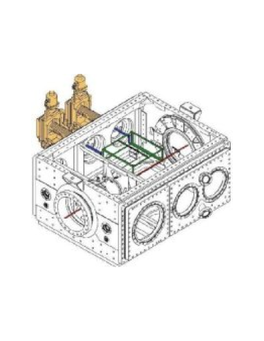
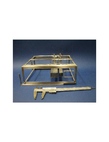
Figure 10: Left: Setup of the movable support for the storage cell inside the new target chamber at ANKE. Right: Support frame, indicated in green on the left panel, with two installed storage cells and a single aperture,. The cross section of the cells are $30\times 20$ mm² and $15\times 15$ mm², the ones of the aperture are $40\times 25$ mm². The unpolarised gas supply to the two cells is attached from the top in the cell centre.

The external positioning control, which is part of the PIT slow–control system, allows one to centre different diaphragms and prototype cells onto the COSY beam axis and to move them step-wise for beam cross section and lifetime studies. According to our preliminary results, a cell tube of about 15 mm diameter (and 350 mm length) can be installed at the beam. However, due to the fact that these measurements had to be done without dedicated COSY beam optimisation and, in view of the strong dependence of the target density upon the lateral extension of the cell tube, further measurements are needed.

These studies have been continued at the beginning of 2005 during one week of beam time allocated for that purpose. During these measurements, the calibrated supply system for unpolarised gases was utilised to feed the storage cell for investigations of e.g. beam-heating effects and for measurements of the pressure distribution in the section in and around the ANKE target chamber. It was possible to inject, store and accelerate to 2.4 GeV/c about $10^{10}$ polarised deuterons in the presence off the large cell, shown on the right panel of Fig. 10. This amounts to about 70% of the number of deuterons that could be stored at injection energy (45 MeV). These test were carried out with a flux of about $10^{-3}$ mbar l/s, leading to a target density in the large cell of $9.4\times 10^{13}$ cm^-2. It was also possible to take the first data from a storage cell target at ANKE in this mode.

4 Beam and Target Polarimetry

4.1 Deuteron beam polarimetry

The polarised $H^{-}$ or $D^{-}$ ion beam delivered by the source [23], is pre-accelerated in the cyclotron JULIC and injected by charge exchange into the COSY ring. The acceleration of vertically polarised protons and deuterons at COSY is discussed in detail for example in ref. [24]. Although beam polarisations in the ring can be established at certain energies by using the EDDA polarimeter [1], in order to ensure that all the conditions of the actual measurement are met, it is preferable to be able to measure oneself the beam polarisation during any experiment. We here describe briefly the first test measurements [25] that were carried out at ANKE using a polarised deuteron beam ($p_{d}=2.4$ GeV/c) and an unpolarised hydrogen cluster target to show how such polarimetry can be carried out in practice.

The scheme for the polarised deuteron beam consisted of eight different polarisation states, including one unpolarised mixture and seven combinations of vector and tensor polarisations. The states and the nominal values of polarisations ($P_{z}$ and $P_{zz}$) and intensities are shown in Table 1. For each injection into COSY, the polarised ion source was switched to a different polarisation state. The duration of a cycle was sufficiently long (200 s) to ensure stable conditions for the injection of the next state. After the seventh state, the source was reset to the zeroth mode and the pattern repeated. The ANKE data acquisition system received status bits from the source, latched during injection, that ensured the correct identification of the polarisation states during the experiment.

Table 1: Modes of the polarised deuteron ion source. The intensity modulations between the different modes constitute a compromise in order to achieve higher polarisations. $I_{0}$ refers to the maximum number of deuterons delivered by the source and stored in COSY.

Figure 11: ANKE experimental acceptance for different reactions in $dp$ collisions at $T_{d}=1170$ MeV.

Fig. 11 shows the ANKE experimental acceptances for singly charged particles for different reactions as functions of the laboratory production angle and magnetic rigidity, together with loci for the kinematics of different allowed processes. The $dp$ elastic scattering reaction has a significant acceptance for $4^{\circ}<\theta_{\textrm{lab}}^{d}<10^{\circ}$. The observables $A_{y}$, $A_{yy}$, and $A_{xx}$ of this reaction were carefully measured at Argonne [26] and SATURNE [27] for $T_{d}=1198$ MeV.

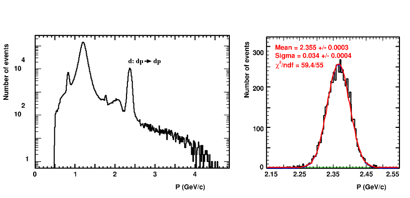
Figure 12: Left: Single–track momentum spectrum for the $dp$ data at 2.40 GeV/c. Right: Fit result of the elastic peak region with the sum of a Gaussian and linear function.

The elastic peak region in the momentum spectrum of the single track events (left panel of Fig. 12) was fitted with the sum of a Gaussian and linear function, and events selected within 3$\sigma$ of the mean. An example of such a fit is shown the right panel.

The $dp\to\,^{3}\textrm{He}\,\pi^{0}$ reaction can be investigated using simply the ${}^{3}\textrm{He}$ information. The high momentum branch of ${}^{3}\textrm{He}$ particles was isolated well in off–line analysis by applying two–dimensional cuts in $\Delta E$ versus momentum and $\Delta t$ versus momentum for individual layers of the forward hodoscope. The tensor analysing power of this reaction has been measured at $0^{\circ}$ as a function of beam energy at Saclay [28].

The quasi–free $np\to d\pi^{0}$ can also be clearly identified by detecting the two final charged particles in the $dp\to p_{sp}d\pi^{0}$ reaction, where $p_{sp}$ is a spectator proton which has about half the beam momentum. Though, by isospin, the differential cross section should be half of that of $pp\to d\pi^{+}$, all the analysing powers should be equal for $\pi^{+}$ and $\pi^{0}$ production.

The charge–exchange process was selected from the missing–mass with respect to the observed proton pairs (see §5.2) and time–difference information. The spectra for all spin modes reveal a well defined peak at M_miss equal to the neutron mass to within 1%. The background was less than $2\%$ and stable, so that the charge–exchange process could be reliably identified.

Using the $\vec{d}p\to\,dp$, $\vec{d}p\to\,(2p)n$, $\vec{n}p\to d\pi^{0}$, and $\vec{d}p\to\,^{3}\textrm{He}\,\pi^{0}$ reactions, which all have large and well known analysing powers, a simultaneous calibration of the vector and tensor components of the polarised deuteron beam at COSY became possible for the first time. In all cases the beam polarisation was consistent with being proportional to the ideal values nominally supplied by the source. The results are therefore summarised in Table 2 in terms of vector and tensor proportionality parameters $\alpha_{z}$ and $\alpha_{zz}$.

Reaction	Facility	$\alpha_{z}$	$\alpha_{zz}$
$\vec{d}p\to dp$	EDDA	$0.74\pm 0.02$	$0.59\pm 0.05$
$\vec{d}p\to dp$	ANKE	$0.73\pm 0.02$	$0.49\pm 0.02$
$\vec{n}p\to d\pi^{0}$	ANKE	$0.70\pm 0.03$	—
$\vec{d}p\to\,^{3}\textrm{He}\,\pi^{0}$	ANKE	—	$0.58\pm 0.05$
$\vec{d}p\to(pp)n$	ANKE	—	$0.48\pm 0.05$

Table 2: Values of vector and tensor polarisation parameters. The errors quoted are only statistical.

The average of the ANKE measurements is $\alpha_{z}^{\textrm{ANKE}}=0.72\pm 0.02$ and $\alpha_{zz}^{\textrm{ANKE}}=0.52\pm 0.03$, which are compatible with EDDA results [29] measured prior to the ANKE run but at lower beam energy and intensity.

4.2 Polarisation export technique

The absolute value of the beam polarisation is clearly needed in any measurement with polarised projectiles. This is usually determined from the scattering asymmetry in a suitable nuclear reaction for which the analysing power is already known. Calibration standards of the type discussed in §4.1 are few and only exist at discrete energies. It is therefore of great practical interest to be able extend their application to arbitrary energies where standards are not yet available. Now, if care is taken to avoid depolarising resonances in the machine, the beam polarisation should in general be conserved during the process of ramping the beam energy up or down [30]. Such tests measurements have been carried out at COSY for both polarised proton and deuteron beams.

Results for proton beam polarimetry are described in ref. [31]. The absence of azimuthal symmetry of the ANKE spectrometer does not permit one to measure a vector analysing power from the left–right count rate asymmetry. We therefore determined $A_{y}$ by reversing the orientation of the polarisation every two cycles. Careful monitoring of the relative luminosity $L_{\uparrow}/L_{\downarrow}$ was achieved by detecting single particles in the FD either at $\theta_{\textrm{lab}}<1^{\circ}$ or at $\phi=90^{\circ}\pm 5^{\circ}$ and $\phi=270^{\circ}\pm 5^{\circ}$, where the rates are insensitive to the vertical beam polarisation.

The beam polarisation at $T_{p}=0.800$ GeV was determined by measuring $pd$ elastic scattering, where the scattering angles were fixed by the energy deposit of the identified deuterons in the silicon telescopes. It should be noted that there are good $pd$–elastic analysing power data at 0.796 GeV [32].

Since the corresponding data are not available at 0.5 GeV, we resorted to the polarisation–export technique [30] to obtain a polarisation calibration. This was achieved by setting up a cycle with a flat top at energy $T_{p}=0.8$ GeV (I), followed by deceleration to a flat top at 0.5 GeV (II), and subsequent re-acceleration to the 0.8 GeV flat top (III). The measured beam polarisations $P_{I}=0.564\pm 0.003^{\mathrm{stat.}}\pm 0.004^{\mathrm{syst.}}$ and $P_{III}=0.568\pm 0.004^{\mathrm{stat.}}\pm 0.005^{\mathrm{syst.}}$ agree within errors, and this shows that we have avoided significant depolarisation while crossing of the resonances. The systematic errors arise from the uncertainties in the relative luminosity. The weighted average of $P_{I}$ and $P_{III}$ was used to export the beam polarisation to flat top II and to determine the angular distribution of the previously unknown analysing power of $pd$ elastic scattering at 0.5 GeV. A small angle–independent correction of $-0.0024$ was applied in the export procedure to account for the 4 MeV difference in beam energy, using the energy dependence of $A_{y}$ between 500 and 800 MeV.

Beam time was allocated in February 2005 in order to measure the polarised $p(\vec{d},pp)n$ reaction at three different beam energies, viz. $T_{d}=1.2$ GeV (for polarimetry purposes), 1.6 GeV, and 1.8 GeV. In order to verify the polarisation export technique with a circulating deuteron beam at COSY, the scheme shown schematically in Fig. 13 was implemented.

Figure 13: Schematic picture of the three different flat-top regions used in a single cycle of the February 2005 run. The identity of the deuteron polarisation in regions I and III means that the 1.2 GeV polarisation could be exported to 1.8 GeV.

The polarimetry was carried out using small angle $dp$ elastic scattering, as described in §4.1. The preliminary results of this test measurement are shown in table 3 in terms of the non–normalised parameters $\beta$ where the analysing power of the reaction has not been introduced. Given that, within the small error bars, $\beta_{y/yy}^{I}=\beta_{y/yy}^{III}$ no depolarisation has been observed. We can therefore conclude that the beam polarisation at 1.8 GeV is the same as that at 1.2 GeV. The export technique can therefore be used for both proton and deuteron beams.

$\beta_{y}^{I}=-0.213\pm 0.005$	$\beta_{y}^{III}=-0.216\pm 0.006$
$\beta_{yy}^{I}=-0.053\pm 0.003$	$\beta_{yy}^{III}=-0.060\pm 0.003$

Table 3: Values of the non–normalised deuteron vector and tensor polarisation parameters obtained before and after beam ramping from 1.2 GeV to 1.8 GeV and back.

4.3 Target polarimetry

Two weeks were granted by the COSY PAC for initial research with the PIT and these are to be scheduled for autumn 2005. The main goal is to accomplish a measurement of the target performance, in particular the target polarisation and density. A suitable reaction to measure the target density is $d\vec{p}$ elastic scattering since, as shown in Fig. 14, the cross section and analysing power have been well studied in the angular range representing the ANKE acceptance [33].

Once the target polarisation has been determined, the data sample obtained can be used to derive the analysing power of the charge–exchange reaction $d\vec{p}\to(pp)n$. However, experience gained during the short test experiment with a polarised deuteron beam and a hydrogen target [34] has shown that the acceptance of ANKE is such that several reactions with well–studied analysing powers will be recorded simultaneously. Among these will be, for example, quasi–free $n\vec{p}\to d\pi^{0}$, which has a fast spectator proton, and $d\vec{p}\to\,^{3}\textrm{He}\,\pi^{0}/\,^{3}\textrm{H}\,\pi^{+}$. There will therefore be several reactions that can be used to provide a calibration.

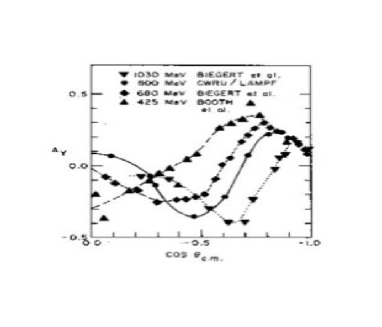
Figure 14: Analysing power data for $d\vec{p}$ elastic scattering [33]. Note that the ANKE acceptance is over the range $-0.77>\cos\theta>-0.98$.

4.4 Luminosity determination

Though this whole document is biassed towards the determinations of analysing powers and spin correlations etc., values of differential cross sections are at least as important and for this the luminosity has to be fixed. Inside a storage ring such as COSY is it customary to do this by measuring in parallel a reaction for which the cross section is known from other experiments. This sometimes limits the energies at which experiments can be reliably standardised. There are, however, two other possibilities that we will exploit for normalisation purposes.

When experiments are carried out using a target cell, the density of the polarised gas target can also be inferred by comparison with detector rates obtained with a calibrated flux of unpolarised hydrogen gas admitted into the centre of the storage cell. This method is described in detail in ref. [35]. More imaginatively, the energy loss of the beam due to electromagnetic interactions in the target is a measure of the integrated luminosity. The energy shift gives rise to a corresponding frequency shift, which can be measured through the study of the Schottky noise spectrum of the coasting beam. It is hoped that this method, which is the subject of a detailed study at COSY [36], will be operational by the end of 2005.

5 Proton–Neutron Spin Physics

The nucleon–nucleon interaction is fundamental to the whole of nuclear physics and hence to the composition of matter as we know it. Apart from its intrinsic importance, it is also a necessary ingredient in the description of meson production processes.

In the case of proton–proton scattering, the data set of differential and total cross sections and the various single and multi–spin observables is very extensive. This allows one to obtain reliable isospin $I=1$ phase shifts up to at least 800 MeV at the click of a mouse [37, 38]. Furthermore, the mass of new high quality EDDA data [1] reduces significantly the $I=1$ phase shift ambiguities up to 2.1 GeV [39]. This is, of course, only possible by taking the new data in conjunction with the results of earlier painstaking systematic work. The meticulous investigation of the nucleon–nucleon interaction must therefore be a communal activity across laboratories, with no single experiment providing the final breakthrough.

Although the extra information required to fix the $I=1$ proton–proton amplitudes uniquely up to 2.1 GeV is limited, the same cannot be said for the isoscalar $I=0$ case, since this would require more good data on neutron–proton scattering. The situation is broadly satisfactory up to around 515 MeV but the only fairly complete data set above that is at the LAMPF energy of around 800 MeV, though many of the measurements were carried out at Saclay [37].

The limited intensity, the large momentum bite, and the general difficulty of working with neutral particles, makes one seek alternatives to using neutron beams for the study of $np$ scattering. For many years the deuteron has been used as a substitute for a free neutron target. The corrections required in order to extract proton–neutron observables are generally quite small and fairly well calculable at high energies because the typical internucleon separation in the deuteron ($\approx 4\>$fm) is large compared to the range of the projectile–nucleon force. It is therefore plausible to assume that the projectile generally interacts with either the target proton or neutron, with the other nucleon being largely a spectator, moving with the Fermi momentum that it had before the collision. Nevertheless, the nature of the corrections have to be studied carefully for each individual reaction. For example, it has been shown that the spin correlation and transfer parameters in $pp$ quasi–elastic scattering in the 1.1 to 2.4 GeV range are very close to those measured in free $pp$ collisions [40] and the Saclay group find exactly the same reassurance for $pn$ quasi–elastic scattering [41]. The investigation was, however, carried out far away from the forward direction whereas other deuteron corrections can be important at small angles, when it is not clear which is the spectator and which the struck nucleon [42].

With the current and projected facilities positioned inside the COSY ring, we expect to contribute to the elastic proton–neutron data base in two distinct regions. By detecting a slow proton in the silicon counters and a fast proton in ANKE, we will measure elastic $pn$ scattering up to the maximum COSY proton beam energy for laboratory angles of the fast proton with $|\theta_{p}^{lab}|<12^{\circ}$ . Using a transversally polarised beam and/or target, this will give access to the unpolarised cross section, $\textrm{d}\sigma/\textrm{d}\Omega$, the proton and neutron analysing powers, $A_{y}$, and the spin correlation parameters, $A_{yy}$ and $A_{xx}$, as described in §5.1.

In parallel with elastic scattering, measurements will also be made of the cross section and spin dependence of the $\vec{p}\,\vec{n}\to d\pi^{0}$ reaction up to 3 GeV by detecting the spectator proton in the silicon counters and the deuteron in ANKE. This reaction [43], which is the prototype of all pion–production processes, can be measured near both the forward and backward cm directions, provided that $|\theta_{d}^{lab}|<8^{\circ}$. This is discussed further in connection with other non–strange mesons in §7.2.1.

The large angle (i.e. charge exchange) region in $np$ elastic scattering is currently being investigated at ANKE by studying the charge exchange reaction of a tensor polarised deuteron beam on an unpolarised target [25, 34]. It has been shown [44] that for low $pp$ excitation energies such experiments are very sensitive to the spin–spin terms in the $np$ charge–exchange amplitude. The deuteron tensor analysing powers are then essentially equivalent to the spin–transfer parameters in $\vec{n}p\to\vec{p}n$. Using both vector and tensor polarised deuterons incident on a polarised hydrogen target, it is possible to investigate additionally both the spin–correlation parameters and triple–spin parameters, such as $A(0s^{\prime};sn)$. More details of this proposal are given in the §5.2.1, where it is seen that one of the biggest drawbacks of this approach is that it is limited by the maximum COSY deuteron energy of $T_{d}\leq 2.3$ GeV, which means that the neutron flux dies out beyond 1.15 GeV.

The same $\vec{p}\,\vec{d}\to ppn$ reaction can, however, be studied in inverse kinematics up to the maximum COSY proton energy of nearly 3 GeV by using a polarised proton beam incident on a polarised deuterium target. The two protons from the reaction then have low energies and both can be very efficiently measured in the silicon telescopes, which cover a significant fraction of the angular domain. It is shown in §5.2.3 that the resolution expected in the $pp$ excitation energy $Q_{pp}$ is even better than that obtainable with a deuteron beam but the price that one has to pay is that very small momentum transfers are not covered for low values of $Q_{pp}$. It should be noted that the magnetic spectrometer is not used when obtaining such data. As a consequence this experiment can be run in parallel with the small–angle $\vec{p}\,\vec{n}$ elastic scattering described in §5.1. In fact, provided that one triggers on at least one low energy proton, relevant data will be accumulated whenever a deuterium target is in position.

At energies well below the pion production threshold, one can model the $NN$ interaction in terms of a purely elastic two–body problem, where the only role played by the mesons is as mediators of the nuclear force [45]. However, at 1 GeV about 40% of the total $np$ cross section corresponds to pion production, mainly involving the excitation of the $\Delta$ isobar. This can be either implicit, as in the $pn\to d\pi^{0}$ reaction to be discussed in §7.2.1, or explicit, as in the $pn\to\Delta^{0}p\to pp\pi^{-}$ reaction. Even below the pion production threshold, such processes give rise to dispersive forces that affect elastic $NN$ scattering [45], though they are sometimes modelled in terms of effective heavy meson exchange. In quark language, the $N\to\Delta$ transition just involves the spin flip of one of the constituent quarks without changing its orbital angular momentum. Any description of the $NN$ interaction above the pion threshold should, at the very least, consider the coupled channels of $NN\rightleftharpoons N\Delta$ [46], for which experimental information is required on the spin dependence of the transition amplitudes.

In addition to detecting the quasi–elastic charge exchange $p(\vec{d},2p)n$ reaction [47, 48], the SPESIV spectrometer allowed the extraction of the strength and analysing power of $\Delta(1232)$ production, $p(\vec{d},2p)\Delta^{0}$, from the missing mass in the reaction [49, 50]. These investigations of the spin–flip excitation of the $\Delta$ will be extended at ANKE with a much bigger $pp$ phase space than at SPESIV, using in addition a polarised hydrogen target. However, an even greater improvement is offered through the use of the polarised deuterium target, which would allow the studies to be pursued all the way up to $T_{p}\approx 3$ GeV. As described in §5.3, the larger missing masses thus accessible would permit also the study of the spin excitation of higher nucleon isobars.

Just as for quasi–elastic charge exchange, the excitation of the $\Delta^{0}$ can be investigated using just the information gathered from the silicon counters. However, further information can be extracted if one measures in ANKE a $\pi^{-}$ or a proton that comes from the decay of the $\Delta^{0}$, viz $\vec{p}\,\vec{d}\to p\,p\,\Delta^{0}\to p_{s}\,p_{s}\,p_{f}\,\pi^{-}_{f}$, where the slow ($s$) and fast ($f$) subscripts indicate where the particles would be detected. In the case of the $\Delta^{0}$, the angular distribution of the decay proton or pion in the $\Delta$ rest frame would determine the alignment of the $\Delta$. In this way we would be measuring some triple–spin observables, which has never been done before for $\Delta$ excitation. The decay pion/proton would also facilitate the separation of the contribution of the $\Delta(1232)$ from those of the other $\pi^{-}p$ resonances.

Small angle elastic proton–deuteron scattering is sensitive to the $I=0$ exchange amplitude, i.e. the sum of the $pp$ and $pn$ amplitudes. Measurements here will therefore provide a qualitatively different check on the phase shifts by removing single pion exchange from the data set. Both polarised and unpolarised data can be taken by detecting the recoil deuteron in the silicon telescopes but, provided that the forward proton does not emerge at too large an angle, the reaction is more clearly identified by measuring also the proton in ANKE.

The physics arguments and the practical implementation of these various programmes, which are listed in Table 4, are reviewed in greater depth in the subsequent subsections.

Table 4: Summary of experiments within the proton–neutron programme. Note that the maximum proton beam energy is almost 3 GeV.

Reaction	Primary detectors	Observables	Kinematic ranges
$\vec{d}\,\vec{p}\to p_{s}p(n)$	ANKE	$\vec{n}\,\vec{p}$ elastic scattering	$0.005<|t|<0.1$ (GeV/c)2
	Si telescopes	$\frac{\textrm{d}\sigma}{\textrm{d}\Omega},\>A_{y},\>C_{nn},\>C_{ss}$
$\vec{p}\,\vec{d}\to p_{s}p(n)$	Si telescopes, ANKE	$\vec{p}\,\vec{n}$ elastic scattering	$4^{\circ}<\theta_{p}^{lab}<11^{\circ}$
		$\frac{\textrm{d}\sigma}{\textrm{d}\Omega},\>A_{y},\>C_{nn},\>C_{ss}$
$\vec{d}\,\vec{p}\to pp(n)$	ANKE	$\vec{n}\,\vec{p}$ charge–exchange	$T_{d}<2.3\>$GeV
		scattering	($T_{p}<1.15\>$GeV)
		$\frac{\textrm{d}\sigma}{\textrm{d}\Omega},\>A_{y},\>C_{nn},\>C_{ss}$	$\theta_{p}^{lab}<7^{\circ}$
$\vec{p}\,\vec{d}\to pp(n)$	Si telescopes	$\vec{p}\,\vec{n}$ charge–exchange	$1.0<T_{p}<2.8$ GeV
		scattering	$|t|<0.25\>$(GeV/c)2
		$\frac{\textrm{d}\sigma}{\textrm{d}\Omega},\>A_{y},\>C_{nn},\>C_{ss}$
$\vec{p}\,\vec{d}\to pp(\Delta^{0})$	Si telescopes	$\vec{p}\,\vec{n}\to\Delta^{0}p$	$0.01<|t|<0.25\>$(GeV/c)2
		$\frac{\textrm{d}\sigma}{\textrm{d}\Omega},\>A_{y},\>C_{nn},\>C_{ss}$
$\vec{p}\,\vec{d}\to ppp\pi^{-}$	Si telescopes, ANKE	$\vec{p}\,\vec{n}\to\Delta^{0}p$	$\theta_{p}^{lab}<12^{\circ}$
		$\frac{\textrm{d}\sigma}{\textrm{d}\Omega},\>A_{y},\>C_{nn},\>C_{ss}$	$|t|>0.01\>$(GeV/c)2
		$A(0s;nn)$
$\vec{d}\,\vec{p}\to dp$	ANKE	$\frac{\textrm{d}\sigma}{\textrm{d}\Omega},\>A_{y},\>C_{nn},\>C_{ss}$	$4^{\circ}<\theta_{d}^{lab}<11^{\circ}$
	Si telescopes, ANKE		$T_{d}<2.3$ GeV
			$0.5<T_{p}<2.8\>$GeV
$\vec{p}\,\vec{d}\to pd$	Si telescopes	$\frac{\textrm{d}\sigma}{\textrm{d}\Omega},\>A_{y},\>C_{nn},\>C_{ss}$	$0.06<|t|<0.46\>$(GeV/c)2
	Si telescopes, ANKE		$|\theta_{p}^{lab}|<12^{\circ}$

5.1 Proton–neutron small angle elastic scattering

To illustrate how proton–neutron elastic scattering can be studied in the small angle region through the combination of the silicon telescopes and the ANKE magnetic analysis, consider the case of a deuteron beam. In Fig. 12 we showed the momentum distribution of charged particles arising from the interaction of 2.4 GeV/c deuterons with a hydrogen target on a logarithmic scale. This yields only two significant peaks. The first around 2.4 GeV/c corresponds to small angle $dp$ elastic scattering whereas the second, close to half the beam momentum, arises from deuteron break–up induced by small angle $pp$ and $np$ scattering. A detailed investigation of the break–up results benefits from information from the silicon telescopes described in §3.3. The subset of events of Fig. 12 where a slow proton was detected in coincidence in the telescope is presented in Fig. 15a on a linear scale. The elastic $dp$ peak is easily eliminated by requiring that the fast particle has a momentum between $0.9$ and $1.5$ GeV/c. These data have as yet been the subject only of a very preliminary analysis [51] and the large corrections arising from final–state–interactions have still to be fully implemented.

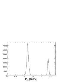
(a) All events

(b) Events that have a momentum of within $\pm 0.3$ GeV/c of half the beam momentum and survive the $\theta_{sp}$ vs $\theta_{fd}$ cut to enhance the $pp$ quasi–elastic reaction.

Figure 15: Momentum distribution of forward-going particles for the Forward–Spectator coincidence trigger.

At large momentum transfers, where one “knows” which particles have taken part in the collision, the cross section is basically the sum of that on the proton and neutron separately with the other particle being a spectator. We first discuss the data in this limiting (classical) picture and return later to the small $q$ region, where quantum mechanical interferences between scattering by the proton and neutron play crucial roles.

The separation of $pp$ from $pn$ quasi–elastic scattering in the classical picture requires us to study the correlation of the polar angles in the forward detector ($\theta_{fd}$) and the spectator counters ($\theta_{sp}$) shown in Fig. 16. Now for elastic $pp$ scattering at a beam energy $T_{p}$ these two angles are related by

$$\tan(90^{\circ}-\theta_{sp})=\left(1+\frac{T_{p}}{2M_{p}}\right)\tan\theta_{fd}\>.$$ (5.1)

Though this relation is shifted slightly by the deuteron binding energy, and smeared significantly by the deuteron Fermi momentum, after taking the counter geometry into account it suggests that the majority of events to the right of the solid line in Fig. 16 corresponds to quasi–elastic $pp$ scattering whereas those to the left arise dominantly from $np$. Events that survive both the momentum and the $pp$ polar angle cuts are illustrated in Fig. 15b.

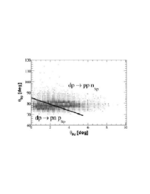
Figure 16: Reconstructed value of the $\theta_{sp}$ angle of the proton in the spectator detector vs the $\theta_{fd}$ of the proton in the forward detector. The solid line indicates the cut chosen to separate the $pn$ and $pp$ quasi–elastic channels.

The corresponding azimuthal angles should also be correlated since for elastic $pp$ scattering one has

$$\phi_{sp}=\phi_{fd}-180^{\circ}\>.$$ (5.2)

The azimuthal correlation is illustrated in Fig. 17a for events where the only selection is that coming from the momentum cut. Since for events where the proton is the spectator there should be essentially no azimuthal correlation, the $pp$ quasi–elastic peak sits on a relatively flat background. This background is almost completely suppressed in Fig. 17b by the imposition of the polar angle cut shown in Fig. 16.

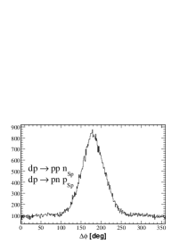
(a) Events surviving the momentum cut

(b) Events surviving both the momentum and $\theta_{sp}$ vs $\theta_{fd}$ cut.

Figure 17: Difference in $\phi$ of the forward–going proton and the proton in the spectator detector. The peak around $180^{\circ}$ originates from the $pp$ quasi–elastic channel and the flat part reflects mainly the $pn$ elastic channel.

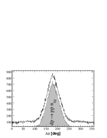
Figure 18: Difference in $\phi$ of the protons in the forward and spectator detectors after applying just the momentum cut and after applying the momentum and $\theta_{sp}$ vs $\theta_{fd}$ cuts. The shaded peak represents mainly the $pp$ quasi–elastic events that have been selected by both cuts.

The comparison of the $\phi$–correlation spectrum with and without the polar angular cut is presented in Fig. 18. This shows a very clean peak which dominantly contains quasi–free $pp\to pp$ events, though it would take a Monte Carlo simulation to try to estimate the neutron contamination. Since the kinematics of each event have been fully identified, one simple consistency test in this classical picture would be to investigate the angular correlations between the slow proton and fast neutron to see if one obtains the same classification of events. This analysis has demonstrated that the silicon telescopes can function well in coincidence with the ANKE magnetic system and that clean data can be obtained in this way.

However, in reality, at low momentum transfers it is not possible even in principle to separate completely the $pp$ from the $pn$ interactions in $dp$ collisions. A naive identification of the slower particle in the deuteron rest frame with the spectator quickly leads to inconsistencies [42]. For small values of $t$ there are coherent effects associated with the addition of the $pp$ and $pn$ amplitudes. Furthermore, much of the transition strength is actually soaked up by the elastic deuteron–proton channel. Such effects are not essentially different in nature from those studied extensively in low momentum transfer deuteron–proton charge exchange [44, 52] and, provided that the $pp$ amplitudes are known, the corrections in the present case depend primarily on the low energy $pn$ final state interaction. Such corrections will be introduced into the analysis of future data taken with the more advanced telescope system with a larger solid angle coverage.

The classical picture fails most spectacularly when both the momentum transfer and the excitation energy in the final $pn$ system is small. In the quasi–free regime there can be no significant dependence of the $\vec{d}p\to(pn)p$ counting rate on the tensor polarisation of the deuteron beam and any such signal would reflect the presence of two nucleons in the deuteron beam. Preliminary values of $A_{yy}$ for the $\vec{d}p\to(pn)p$ reaction with $E_{pn}\leq 5\,$MeV are shown in Fig. 19. The signal is large and negative, though this decreases in strength as the cut on $E_{pn}$ is relaxed while the vector analysing power increases in this limit.

Figure 19: $A_{yy}$ of the $\vec{d}p\to(pn)p$ reaction at $T_{d}=1170\,$MeV for events where $E_{pn}<5\,$MeV in bins of momentum transfer $q$. Also shown is the interpolation of the analysing power of the charge–exchange data of Fig. 25 where account has been taken of the dilution caused by the finite $\phi$ acceptance. Both curve and points are subject to a common overall normalisation uncertainty of 4% arising from the beam polarisation.

In the figure we show also a parameterisation of the $p(\vec{d},2p)n$ tensor analysing power $A_{yy}$ of Fig. 25, where account has been taken of the signal dilution due to the finite azimuthal acceptance in the $(pn)$ case. At the smallest momentum transfer ($q\approx 80\,$MeV/c), $A_{yy}(\vec{d}p\to\{pn\}p)\approx A_{yy}(\vec{d}p\to\{pp\}n)$, though the values diverge as $q$ is increased. This is not an accident! If we neglect the deuteron $D$–state then in impulse approximation at $q=0$ the only allowed transition in the $\vec{d}p\to(pn)p$ reaction is ${}^{3}\!S_{1}\to\,^{1}\!S_{0}$. This has a $(\Delta S,\,\Delta I,\,\Delta I_{z})=(1,\,1,\,0)$ character and is just the isobaric analogue of the deuteron charge–exchange reaction discussed in §5.2. Furthermore, the $(0,\,0,\,0)$ transitions, driven by the large isoscalar spin–non–flip $NN$ amplitudes, vanish like $q^{4}$ at small $q$. This is because they correspond to final ${}^{3}\!D_{1}$ or higher $S$–waves that are orthogonal to the deuteron wave function. The only possible source of dilution of the $A_{yy}$ signal to order $q^{2}$ arises therefore from the ${}^{3}\!S_{1}\to\,^{3}\!P_{0,1,2}$ transitions, which also involve an isospin flip. The final transition to this order is ${}^{3}\!S_{1}\to\,^{1}\!P_{1}$, which is isoscalar.

This picture will, of course, have to be modified somewhat to take into account effects arising from the deuteron $D$–state. However, the basic suppression of the scalar–isoscalar amplitude at small $q$ remains and this does explain qualitatively our findings that $A_{yy}(\vec{d}p\to\{pn\}p)$ looks like a diluted charge–exchange signal and that $A_{y}$, which should vanish for the ${}^{1}\!S_{0}$ state [44], increases for larger $q$ and $E_{pn}$ through the excitation of the ${}^{3}\!P_{0,1,2}$ system.

5.2 Proton–neutron elastic charge exchange

The ANKE collaboration is making measurements of the $\vec{d}p\to ppn$ reaction with the aim of extracting spin–dependent $np$ charge–exchange amplitudes [25, 34].

Now the most complete investigation of deuteron charge exchange in the COSY energy regime was carried out at Saclay at 1.6 and 2.0 GeV [47, 48] and the results for the hydrogen and deuterium targets are shown in Fig. 20. Because of uncertainties in the acceptance of the SPESIV spectrometer used in the experiment to detect the pairs of protons, the overall cross section normalisation is arbitrary, though the relative strength between deuterium and hydrogen targets away from the forward direction is $0.68\pm 0.04$. At $q\approx 0$, it is reduced by a further factor of about $2/3$ due to the Pauli blocking the final $nn$ system.

 

Fig. 20: Cross section and Cartesian and spherical tensor analysing powers of the $(\vec{d},2p)$ reaction on hydrogen and deuterium at $T_{p}=1.6$ GeV [48]. The broken curves represent plane–wave predictions whereas the solid ones include eikonal corrections [53]. The overall cross section normalisation was chosen to agree with theory at a momentum transfer of $q=0.7$ fm^-1.

To show the basic sensitivity of these measurements, consider neutron–proton charge–exchange amplitudes in the cm system:

$$f_{np}=\alpha+i\gamma({\mbox{\boldmath$\sigma$}}_{n}+{\mbox{\boldmath$\sigma$}}_{p}){\bf n}+\beta({\mbox{\boldmath$\sigma$}}_{n}\cdot{\bf n})({\mbox{\boldmath$\sigma$}}_{p}\cdot{\bf n})+\delta({\mbox{\boldmath$\sigma$}}_{n}\cdot{\bf m})({\mbox{\boldmath$\sigma$}}_{p}\cdot{\bf m})+\varepsilon({\mbox{\boldmath$\sigma$}}_{n}\cdot{\bf l})({\mbox{\boldmath$\sigma$}}_{p}\cdot{\bf l}),$$ (5.3)

where ${\mbox{\boldmath$\sigma$}}_{n}$ and ${\mbox{\boldmath$\sigma$}}_{p}$ are the Pauli matrices for neutron and proton, respectively. The orthogonal unit vectors are defined in terms of the initial (${\bf k}$) and final (${\bf k}^{\prime}$) momenta as

$$\mathbf{n=\frac{\mathbf{k}\times\mathbf{k^{\prime}}}{|\mathbf{k}\times\mathbf{k^{\prime}}|},~{}~{}m=\frac{\mathbf{k^{\prime}}-\mathbf{k}}{|\mathbf{k^{\prime}}-\mathbf{k}|},~{}~{}l=\frac{\mathbf{k^{\prime}}+\mathbf{k}}{|\mathbf{k^{\prime}}+\mathbf{k}|}\,.}$$

The amplitudes are normalised such that the elementary $np\to pn$ differential cross section has the form

$$\left(\frac{d\sigma}{dq^{2}}\right)_{\!\!np\to pn}=I_{np}=|\alpha|^{2}+|\beta|^{2}+2|\gamma|^{2}+|\delta|^{2}+|\varepsilon|^{2}.$$ (5.4)

For low excitation energy $E_{pp}<3$ MeV of the final $pp$ pair, and at low momentum transfer, the charge exchange reaction $dp\to(pp)n$ mainly excites the ${}^{1}S_{0}$ state of the final $pp$ system, which involves a spin–flip from $np$ triplet to $pp$ singlet. The process therefore provides a spin–filter. In single–scattering approximation, the resulting amplitude depends only upon the spin–dependent parts of $f_{np}$, i.e. $\beta$, $\delta$ and $\varepsilon$. Bugg and Wilkin [44] have shown that, under these conditions, there are two form factor describing the transition from the deuteron to the ${}^{1}S_{0}$ $pp$ state:

$$S^{+}(k,\mbox{${\textstyle\frac{1}{2}}$}q) = \langle\psi_{k}^{(-)}|j_{0}(\mbox{${\textstyle\frac{1}{2}}$}qr)|u\rangle+\sqrt{2}\langle\psi_{k}^{(-)}|j_{2}(\mbox{${\textstyle\frac{1}{2}}$}qr)|w\rangle\,,$$

$$S^{-}(k,\mbox{${\textstyle\frac{1}{2}}$}q) = \langle\psi_{k}^{(-)}|j_{0}(\mbox{${\textstyle\frac{1}{2}}$}qr)|u\rangle-\langle\psi_{k}^{(-)}|j_{2}(\mbox{${\textstyle\frac{1}{2}}$}qr)|w\rangle/\sqrt{2},$$ (5.5)

where $u(r)$ and $w(r)$ are the $S$ and $D$ components of the deuteron wave function and $\psi^{(-)}_{k}(r)$ is the $pp$ $(^{1}\!S_{0})$ scattering wave function. Here $k$ is the $pp$ relative momentum, corresponding to an excitation energy $E_{pp}=k^{2}/M$, where $M$ is the proton mass. Denoting the ratio of the transition form factors by $R=S^{+}(k,\mbox{${\textstyle\frac{1}{2}}$}q)/S^{-}(k,\mbox{${\textstyle\frac{1}{2}}$}q)$ and the sum of squared amplitudes

$$I=|\beta|^{2}+|\gamma|^{2}+|\varepsilon|^{2}+|\delta|^{2}R^{2},$$ (5.6)

the differential cross section, tensor analysing powers, and transverse spin–spin correlation parameters of the $dp\to(pp)_{{}^{1}S_{0}}n$ reaction take the forms [44, 54]

$$\frac{d^{4}\sigma}{dq^{2}d^{3}k} = \mbox{${\textstyle\frac{1}{3}}$}I\left\{S^{-}(k,\mbox{${\textstyle\frac{1}{2}}$}q)\right\}^{2},$$

$$I\,T_{20} = \mbox{${\textstyle\frac{1}{\sqrt{2}}}$}\{|\gamma|^{2}+|\beta|^{2}+|\delta|^{2}R^{2}-2|\varepsilon|^{2}\}$$

$$I\,T_{22} = \mbox{${\textstyle\frac{\sqrt{3}}{2}}$}\{|\gamma|^{2}+|\beta|^{2}-|\delta|^{2}R^{2}\}$$

$$I\,C_{x,x} = -2\textrm{Re}(\beta^{*}\varepsilon)$$

$$I\,C_{y,y} = -2\textrm{Re}(\varepsilon^{*}\delta)R.$$ (5.7)

After rotating these formulae for the $T_{2i}$ to the beam direction [55], they were used by the Saclay group [48] to interpret their data at 1.6 GeV. The only significant correction comes from the multiple scatterings whose effects increase steadily with momentum transfer [44].

However, it is important to stress that data at larger $pp$ excitation energies also contain valuable information on the $pn$ charge–exchange amplitudes [56], but for this a detector of much larger acceptance than SPESIV is required. This was provided at low beam energies by the EMRIC device, which determined the cross section, tensor, and vector analysing powers at 200 and 350 MeV [57]. These agreed well with impulse approximation estimations [52] and provided the basis for the design of the POLDER polarimeter [58]. This has been used very successfully in the determination of the polarisation of the recoil deuteron in elastic electron–deuteron scattering at J–Lab, which allows the separation of the deuteron form factors [59].

By design, the above $(\vec{d},2p)$ experiments were carried out at energies where the $np\to pn$ amplitudes are relatively well known [37]. The aim of COSY proposal 125 [25] is to carry out such measurements at energies where the $np$ data base is far less complete, in particular above the Los Alamos energy of 800 MeV per nucleon. Furthermore, by using polarised beam and targets, one can gain access also to spin–correlation parameters, which contain valuable relative phase information. Such experiments can be carried out using a polarised deuteron beam, as is currently being employed [25], or a polarised deuterium target and we now compare the merits of the two approaches.

5.2.1 Charge–exchange with a polarised deuteron beam

An initial measurement of the deuteron–induced charge–exchange reaction was carried out at the ANKE spectrometer using a polarised deuteron beam at $p_{d}=2400$ MeV/c ($T_{d}=1170$ MeV) [25]. Two fast protons, emitted in a narrow forward cone with momenta around half that of the deuteron beam, were detected by the Forward Detector (FD) system of the ANKE set–up (see fig 11).

Figure 21: a: Correlation of the momenta of two charged tracks in ANKE resulting from the interaction of 1.17 GeV deuterons in a hydrogen target. b: Correlation of the time differences $\Delta t_{meas}$ and $\Delta t_{tof}$.

The first step in processing the $dp$ charge–exchange breakup data is to choose two–track events using the MWPC information. The momentum vectors were determined with the help of the magnetic field map of the spectrometer, assuming a point–like source placed in the centre of a beam–target interaction region. Fig. 21a displays double–particle events on a scatter plot of particle momenta $p_{1}$ versus $p_{2}$. The smallness of the FD solid angle acceptance leads to a kinematic correlation for events with two or three particles in the final state (Fermi motion spreads slightly the correlation for the corresponding quasi–free processes). No assumption on the masses of the particles is required for such a correlation. The break–up events clearly manifest themselves among several processes recorded in the spectrometer. For the events with particles hitting different counters in the hodoscope, the correlation of a measured time difference $\Delta t_{meas}$ with a difference of the time of flight $\Delta t_{tof}$ can be observed. The time of flight from the target to the hodoscope is calculated from the measured momentum assuming that the particle has the mass of the proton mass. Real proton pair events are then located at the diagonal of the scatter plot (Fig. 21b).

Figure 22: Missing mass distribution of all observed proton pairs. The inset shows the distribution near the neutron mass for the pairs selected by the TOF.

The charge–exchange process was identified from the missing–mass with respect to the observed proton pairs (see Fig. 22) and time difference information. The spectra for all spin modes reveal a well defined peak at M_miss equal to the neutron mass to within 1%. The background was less than $2\%$ and stable, so that the charge–exchange process could be reliably identified.

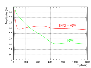
(a) Moduli of the two independent $np\to pn$ scattering amplitudes at $t=0$.

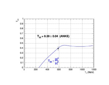
(b) $T_{20}$ for $\vec{d}p\to(pp)_{{}^{1}\!S_{0}}n$ in impulse approximation compared to our value of $T_{20}=0.39\pm 0.04$ at $\frac{1}{2}T_{d}=585$ MeV.

Figure 23: Predictions for amplitudes and observables deduced using the SAID program [37].

Using the polarised deuteron charge–exchange (CE) break–up reaction $p(\vec{d},2p)n$, where the final protons have an excitation energy of less than 3 MeV and hence are in the ${}^{1}\textrm{S}_{0}$ state, we can access the spin–dependent amplitudes of the elementary $np$ elastic scattering using Eq. (5.7). For collinear kinematics we can directly reconstruct the magnitude of the two spin amplitudes by measuring the cross section and $T_{20}$ analysing power. The value of the ratio $|\beta(0)|/|\varepsilon(0)|=1.86\pm 0.15$, obtained from our preliminary experiment, is shown in Fig. 23. Also shown are predictions for the values of the moduli of the two forward spin–flip amplitudes, as functions of energy [37]. Since the SAID prediction of the ratio is $1.79\pm 0.27$ [37, 60], it is clear that our statistical precision is already superior to that of the World data base.

Though the angular acceptance for the two fast protons in ANKE is very limited, it is known that the tensor analysing powers should change very fast with momentum transfers due to the near–vanishing of the $\delta$ amplitude for $q\approx m_{\pi}$ [44]. It is then possible to utilise the dependence of the signal on the azimuthal angle to extract separately values of $T_{20}$ and $T_{22}$, or the Cartesian analysing powers $A_{yy}$ and $A_{xx}$, and preliminary estimates are to be found in 20 MeV bins in momentum transfer in Figs. 24 and 25 respectively. If the excitation energy is not cut sufficiently, these tensor signals should be diluted slightly at larger $q$ due to contamination from final spin–triplet states [44]. As seen from the figures, the effects of changing the limit on $E_{pp}$ from 1 MeV to 3 MeV is only significant above about 100 MeV/c. The value in the final bin is just compatible with the kinematic limit $A_{xx}\leq 1$. Also illustrated in Fig. 25 are the $A_{yy}$ results from SATURNE at the rather higher energy of 1600 MeV [48]; at these small values of momentum transfer this group did not have a clean separation of $A_{xx}$ and $A_{yy}$.

The variation with momentum transfer is generally as expected on the basis of the Bugg–Wilkin model [44] though the detailed theoretical calculation [52], as used to describe data at lower energies [57], has still to be implemented at our energy.

Figure 24: Spherical tensor analysing powers $T_{20}$ and $T_{22}$ of the $p(\vec{d},2p)n$ reaction at $T_{d}=1170\,$MeV in 20 MeV bins of momentum transfer $q$ with two different cuts on the excitation energy: $E_{pp}<1\,$MeV (blue) and $E_{pp}<3\,$MeV (red).

Figure 25: Cartesian tensor analysing powers $A_{yy}$ and $A_{xx}$ of the $p(\vec{d},2p)n$ reaction at $T_{d}=1170\,$MeV with cuts as in Fig. 24. Also shown by stars are the $A_{yy}$ measurements from SATURNE at 1600 MeV [48].

5.2.2 Polarimetry reactions

To illustrate the power of the spectrometer in identifying two–body and quasi–two–body reactions, many of which are used to calibrate the beam polarisation, we show some of the results obtained in polarised deuteron–proton collisions at $T_{d}=1.17$ GeV [25, 34]

Fig. 11 showed the ANKE experimental acceptances for singly charged particles for different reactions as functions of the laboratory production angle and magnetic rigidity, together with the loci representing the kinematics of different allowed reactions.

To facilitate the subsequent discussion, we show in Fig. 26 kinematic curves relating the laboratory and cm angles for three observed two–body reactions, viz: $dp\to dp$, $dp\to\,^{3}\textrm{He}\,\pi^{0}$, and $np\to d\pi^{0}$ at the momentum of the 2004 run (2.435 GeV/c) [34] and also at the higher COSY momentum (3.463 GeV/c). From these it is seen that the $dp\to dp$ reaction has a significant acceptance for $4^{\circ}<\theta_{lab}^{d}<10^{\circ}$, and that this depends little on the beam momentum.

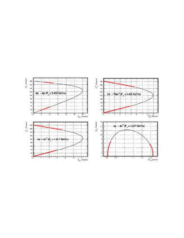
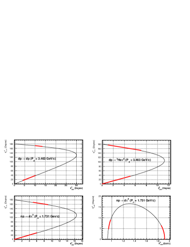
Figure 26: Kinematic curves for different reactions at deuteron momenta of 2.435 and 3.463 GeV/c; the bold parts of the curves denote regions accessible in the current set–up.

The quasi–free $np\to d\pi^{0}$ can be clearly identified in ANKE through the detection of the two final charged particles in the $dp\to p_{sp}d\pi^{0}$ reaction, where $p_{sp}$ is a spectator proton which has essentially half the beam momentum, $p_{sp}\approx 1.17$ GeV/c [34]. In the two–dimensional momentum spectrum of Fig. 21 are shown the bands arising from the high ($p_{d}\approx 1.3$ GeV/c) and low–momentum ($p_{d}\approx 0.8$ GeV/c) branches, corresponding to backward and forward production of the $\pi^{0}$ in the cm system.

The two–dimensional spectrum in the differences of the times of flight shown in Fig. 21 proves that there is in fact very little background for these events, and this is supported by the missing masses for the two regions in Fig. 27, which demonstrates well identified pion peaks, though the single run presented here represents but a small part of our overall statistics.

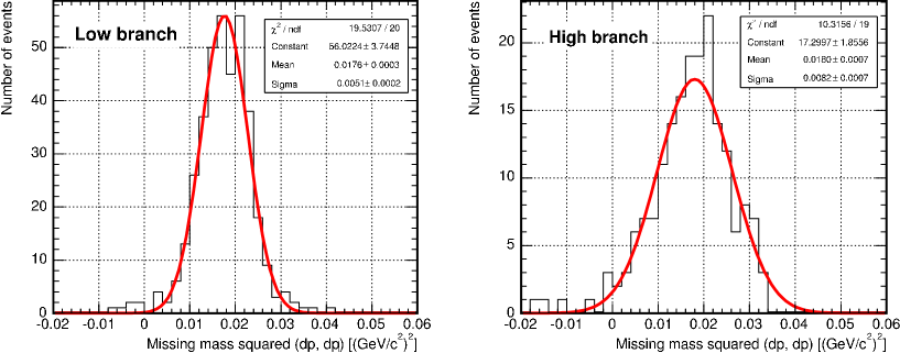
Figure 27: Missing masses from the $\vec{d}p\to p_{sp}dX$ reaction showing clear $\pi^{0}$ peaks.

The two–dimensional plot of data on the deuteron production angle versus momentum is shown in Fig. 28, where it is seen that results from both the high and low–momentum branches are scattered around the kinematical curve corresponding to the free $np\to d\pi^{0}$ reaction.

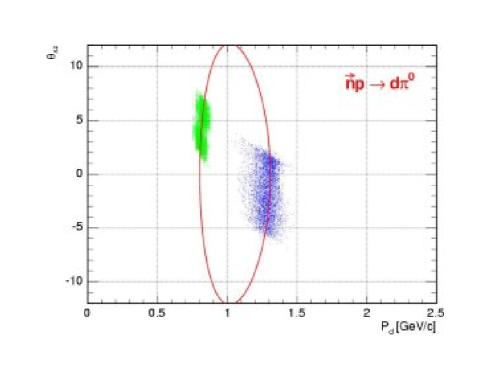
Figure 28: $\theta_{d}$ versus $p_{d}$ scatter plot compared with the kinematic locus for the free $np\to d\pi^{0}$ reaction.

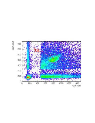
(a) ³He identification

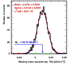
(b) Missing mass squared for the reaction $dp\to\,^{3}\textrm{He}\,X$. The result of the peak fit is indicated.

Figure 29: Identification of the $dp\to\,^{3}\textrm{He}\,\pi^{0}$ reaction.

In the $dp\to\,^{3}\textrm{He}\,\pi^{0}$ case, the $\pi^{0}$ is recognised through the missing mass obtained from the ${}^{3}\textrm{He}$ measurement. The result of this identification is shown in Fig. 29. The high momentum branch of ${}^{3}\textrm{He}$ particles was selected well in off–line analysis by applying two–dimensional cuts in $\Delta E$ versus momentum and $\Delta t$ versus momentum for individual layers of the forward hodoscope. Though the peak in Fig. 29 is wide, this is not critical since, apart from the radiative capture, there is no physical background over this region.

5.2.3 Charge–exchange with a polarised deuterium target

The advantages of studying charge exchange using just the spectator counters in combination with a polarised deuterium target have already been outlined. Preliminary Monte Carlo simulations of the acceptances in momentum transfer versus $pp$ excitation energy are to be found in Fig. 30 for both elastic and $\Delta$ production in charge exchange of protons with momenta 1.7 and 3.0 GeV/c. Both protons are given Fermi momentum distributions and the $pp$ fsi is included, but no attempt has yet been made to include a dynamic reaction mechanism.

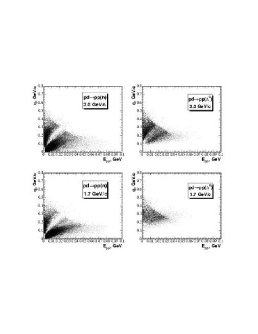
Figure 30: Simulations of the acceptances for elastic and inelastic charge exchange on a deuterium target where the two protons are detected in the spectator counters.

The details of the plots will depend critically upon the placing of the silicon detectors and the values shown here are obtained using the configuration described in §3.3. Nevertheless, several features are common to different settings. The wide valley with no counts, running from the bottom left corner, indicates the separation of the regions where the two protons go into the same or different counters. If they go into the same counter at low $E_{pp}$ a minimum momentum transfer is required in order to give an energy sufficient to separate the signals (typically 1 MeV). When the protons go into different telescopes, it is not possible to get very small momentum transfers and so in the elastic case there is a blind area when both $E_{pp}$ and $q$ are small. The cut–off when these variables are both large is connected with the maximum stopping power of the silicon detectors, here assumed to be 60 MeV. There are still some events in the $S$–wave region of $E_{pp}<3$ MeV but, as shown in Fig. 31, it is not possible to follow the $q$–dependence of these very far.

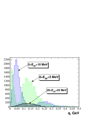
Figure 31: Projections of the $pd\to ppn$ acceptance of Fig. 30 at 3.0 GeV/c.

In the case of inelastic charge exchange, there is a minimum longitudinal momentum transfer set by the kinematics of $q_{min}\approx(M_{\Delta}^{2}-M_{n}^{2})/2p_{lab}$, where $p_{lab}$ is the laboratory beam momentum. Until one gets well above this lower bound, at least one of the protons is likely to go to far forward and miss the spectator counters. This problem gets worse at lower momenta.

5.3 Proton–neutron inelastic charge exchange

It was argued earlier that for energies somewhat above the pion production threshold, it is hard to treat the $NN$ interaction in isolation and that one must consider at least the coupling to the $N\Delta$ channel [46]. The number of amplitudes, the width of the $\Delta$ and the associated difficulty of overlapping bands in the Dalitz plots, and the weaker constraints provided by unitarity, make this problem very challenging indeed, both experimentally and theoretically. We believe, however, that COSY can make significant contributions in this field. This is important because serious problems arise when phenomenological $NN\to N\Delta$ amplitudes are used as input for the estimation of spin–observables in more complicated reactions. For example, the inclusion of three–body forces arising from $\Delta$–excitation [61, 62] improve the agreement between Faddeev calculations and the unpolarised differential cross section for $dp$ elastic scattering at $T_{p}<200$ MeV. However there is no corresponding systematic improvement for the spin–observables measured in this process. A deficit in our knowledge of the spin structure of the three–body forces was pointed out recently in $pd\to(pp)n$ at 0.5 GeV [31].

The first amplitude analysis of $NN\to N\Delta$ was reported by Wicklund et al. [63]. The subsequent analysis of Shypit et al. [64] used only data from their own experiment but this was followed by an update [65] that included all the World data available at that time, i.e.

1. $\textrm{d}\sigma/\textrm{d}\Omega$, $A_{N0},A_{S0}$ and $A_{L0}$ near 576 and 792 MeV [63]

2. $\textrm{d}\sigma/\textrm{d}\Omega$ and $A_{N0}$ at 800 MeV [66],

3. $A_{NN}$ and $A_{LL}$ at 643, 729 and 800 MeV [67],

4. Five Wolfenstein parameters at 643, 729 and 800 MeV [68, 69],

5. $\textrm{d}\sigma/\textrm{d}\Omega$, and $\sigma_{inel}$ over the complete energy range [70].

It also included $\pi N$ partial waves $S_{31}$, $S_{11}$, $P_{31}$, and $P_{11}$ using the OPE approximation for $NN\to N(\pi N)$. The amplitude analysis of $pp\to d\pi^{+}$ and $pp\to N\Delta$ from Ref. [65] was used in Ref. [71] as input to perform a re-analysis within the $N/D$ method. The aim was to distinguish between the pole or cusp interpretation of the data near the $N\Delta$ threshold.

Let us discuss in more detail, for example, the Argonne data [63], which were obtained at proton beam energies of 0.57, 0.81, and 1.01 GeV, and the first amplitude analysis of these results. In Ref. [72] the data on the $NN\to N\Delta$ reaction were investigated within the unitary model of coupled $\pi NN-NN$ channels. This model, based on the meson–exchange picture, describes in a unified manner the following processes: $NN\to NN$, $NN\leftrightarrow\pi d$, $NN\leftrightarrow\pi NN$, $\pi d\to\pi d$, and $\pi d\to\pi NN$. The unpolarised differential cross section, production asymmetry and spin correlation parameters were calculated for the $NN\to N\Delta$ reaction. The global agreement with the available Argonne data is reasonably satisfactory. The main problem concerns the integrated asymmetry $A_{y}$, which is consistent with the data only at 0.57 GeV. At higher energies, the model is unable to reproduce the change from a broad positive maximum to the broad positive minimum observed in $A_{y}$. The asymmetry problem at high energy is directly related to the fact that none of the models used is able to describe the helicity–$3/2$ spin–correlation parameter $P_{y}\rho_{33}$.

A possible way to improve (partially) the agreement was pointed out in Ref. [73], where the $NN\to N\Delta$ amplitude was extracted from the Bonn meson–exchange model of elastic $NN$–scattering. Within such a model of the $NN$–interaction, taking account of the coupling to the $N\Delta$ and $\Delta\Delta$ channels allows one to improve considerably the phase shifts and inelasticity parameters of $NN$–scattering below 1 GeV [39]. At higher energies, only the $NN$ total and integrated elastic cross sections are satisfactorily described with Reggeised vector meson exchanges, whereas the spin observables measured at 1–2.5 GeV are in strong disagreement with the OBE model predictions. However, the Bonn model does not take into account the correlated $2\pi$ and $\pi\rho$ exchanges, which are included in the Jülich model [74]. The polarised deuteron charge–exchange programme of the Saclay group included some measurements of the excitation of $\Delta(1232)$ through the $\vec{d}A\to pp\,A^{\prime}$ reaction for targets $A=p,\,d,\,^{12}$C, where the isobar was identified via the missing mass in the reaction [49, 50]. The near–forward differential cross sections for hydrogen and deuterium targets are shown in Fig. 32 at $T_{d}=2\>$GeV as functions of the laboratory energy loss $\omega_{lab}$. To a good approximation, the polarisation response is related to the analysing power by $A_{yy}\approx-\sqrt{2}P/\rho_{20}$, where the beam polarisation $\rho_{20}=0.61\pm 0.01$. As mentioned in §5.2.3, quasi–elastic charge exchange on deuterium was a factor of about $0.68$ smaller than for hydrogen. However, in the pion–production region, the quasi–free $dd\to pp\Delta^{-}p$ cross section should be bigger than that for $dd\to pp\Delta^{0}n$ by an isospin factor of three. The polarisation responses are essentially indistinguishable and, when the deuterium data are divided by a factor of $4\times 0.68$, the hydrogen and deuterium results largely coincide. This agreement with the scaled cross sections is similar Fig. 32: Polarisation response and cross section for $p(\vec{d},2p)\Delta^{0}$ and $d(\vec{d},2p)\Delta N$ at $T_{d}=2\>$GeV and $\theta_{pp}^{lab}=0.5^{\circ}$. The broken histogram corresponds to the scaled result for deuterium. The solid curves are models with direct pion exchange whereas for the broken curves this is modified using the poor man’s absorption model cut off [50].

at the other angles measured and this proves the expected dominance of the $I=\frac{3}{2}$ strength.

Unlike the $p(\vec{d},2p)n$ measurements at 1.6 GeV, discussed in the previous subsection, no spin–rotator was used for $\Delta$ excitation at 2.0 GeV. On account of the small angular acceptance of SPESIV, only one tensor analysing power combination could then be measured and this principally determined $A_{yy}$.

Away from the forward direction, the poor man’s absorption prescription to the one–pion exchange model for $pN\to\Delta N$ gives a plausible description of the cross section and analysing power [50]. However, the density matrix elements for the $\vec{p}\,p\to\Delta^{++}n$ reaction at the rather higher energy of $T_{d}=2.2\>$GeV [63], which depend upon interference terms, are only qualitatively reproduced. Inelastic charge–exchange experiments will be repeated at ANKE in the near future with a polarised deuteron beam of a similar energy to Saclay as a by–product of the approved $p(\vec{d},2p)n$ experiment [25, 34]. A wider range of different deuteron analysing powers will then be derived. Already in Fig. 22 we see some evidence of pion production even at $T_{d}=1.17$ GeV.

In the future it will be possible to go to much higher energies by using the polarised deuterium internal target. Though there is little chance of getting sufficient data in order to allow a completely model–independent amplitude analysis,and the phase space shown in §5.2.3 is limited, we will measure the $\vec{d}(\vec{p},2p)\Delta^{0}$ reaction with polarised beam and target up to $T_{p}\approx 3\>$GeV, using just the spectator telescopes in the manner described in the previous subsection. Rank–two tensor observables, such as the $t_{20}$ and $t_{22}$ analysing powers and the transverse spin–correlation coefficient of the proton with a vector polarised deuteron, are particularly robust quantities that can pick out moduli of amplitudes rather than the imaginary parts of interferences that are sensitive to phase differences which can arise from the $NN$ or $N\Delta$ interactions.

However, the tensor polarisation of the outgoing $\Delta^{0}$ can also be measured, as was demonstrated at Argonne for the $\vec{p}\,p\to\Delta^{++}n$ reaction, by looking at the angular distribution of the pion or proton from the $\Delta$ decay in the $\Delta$ rest frame [63]. In our case, this would require the detection in ANKE of the fast $\pi^{-}$ or proton from the $\Delta^{0}$ disintegration in coincidence with the two slow protons in the silicon counters. Now for the $NN\to\Delta N$ reaction there are four independent amplitudes in the forward direction and it can be shown [75] that study of the $\vec{d}\vec{p}\to(pp)\vec{\Delta}^{0}$ reaction will give access to three combinations of these amplitudes.

In small momentum transfer reactions, such as this and $p(d,2p)n$, it is to be expected that the major correction to a simple quasi–free interpretation will come from multiple scatterings, which can be handled in the eikonal approximation [53]. These generally give an overall damping and have less effect on the spin observables until the momentum transfers are above around $1\>$fm^-1 [48, 50]

5.4 Small angle $\vec{p}\,\vec{d}$ or $\vec{d}\,\vec{p}$ elastic scattering

Elastic proton–deuteron scattering at small angles can be measured at ANKE with a deuteron beam or a deuterium target but the kinematic ranges will differ. With a proton beam one could detect a deuteron in the spectator counters and a proton in the FD and, observed in this way, the reaction has already been used for luminosity and beam polarisation determinations at ANKE [31]. However, the cross section is so big that merely measuring the deuteron in the spectator counters is sufficient to identify completely the process. Considering only recoil deuterons with energies in the range $2.5<T_{d}<50$ MeV leads to the plot of the minimum and maximum proton cm angles shown in Fig. 33. This corresponds essentially to a fixed range in momentum transfer, $0.001<|t|<0.19$ (GeV/c)², which we can cover up to the maximum COSY energy of close to 3 GeV.

Figure 33: Predicted upper and lower bounds on the proton cm angle in proton–deuteron elastic scattering, with only the deuteron being detected in the silicon telescopes.

Above about 1.5 GeV the fast proton would fall within the maximum ANKE angular acceptance of $\theta_{p}^{lab}<11^{\circ}$ but even then some of the small momentum transfer protons would be lost in the forward cone of $\theta_{p}^{lab}<4^{\circ}$.

Small angle deuteron–proton elastic scattering has also been measured at COSY by detecting just the deuteron in the ANKE magnetic spectrometer. It could be used for luminosity and polarisation purposes [34] since, as shown in Fig. 12, the proton does not need to be measured in order to have a very clean signal for the reaction. The acceptance for measuring the deuteron from the reaction at $T_{d}=1170$ MeV can be deduced from Fig. 11 and, as shown in Fig. 26, this remains roughly the same in the laboratory at different beam momenta; $4^{\circ}<\theta_{d}^{lab}<10^{\circ}$.

Comparing the acceptances for $pd$ and $dp$ elastic scattering, it is seen that smaller angles are covered with the proton beam. This illustrates the power of the silicon telescope array when used at the ANKE facility.

6 Proton–Deuteron Reactions at High Momentum Transfers

The combination of the ANKE magnetic spectrometer and spectator telescopes with polarised beams and a polarised deuterium gas cell will lead to the detection in parallel of many non–mesonic nuclear reactions in addition to those in the proton–neutron programme outlined in §5. Some of these have a great interest in their own right and will require dedicated beam time if their potential is to be exploited to the full. This is especially true of large momentum transfer proton–deuteron elastic and charge exchange scattering, for which interesting results have already been achieved at low $pp$ excitation energies at ANKE [76, 31].

The nuclear three–body problem is fundamental, but the difficulty that one faces with such studies at ANKE is that the main benefits of COSY come when working above the pion–production threshold. This is a region where, for a variety of reasons, the Faddeev description of proton–deuteron elastic and inelastic reactions is no longer appropriate. There is then no agreed calculational scheme to model such data and there is much ambiguity in how to interpret, for example, the energy dependence of the cross section and tensor analysing power of $dp$ elastic scattering at $180^{\circ}$ [77], though virtual $\Delta$ excitation is certainly involved at some level [78, 79]. Nevertheless, it is hoped that the measurement of spin observables will provide valuable clues to the dominant reaction mechanisms involved. As an example of this, consider the $\vec{p}d\to(pp)_{\!{}^{1}\!S_{0}}n$ reaction, where it has been shown that at 500 MeV the proton analysing power is almost maximal for $\theta_{n}^{cm}\approx 167^{\circ}$ [31]. This indicates that, out of the six possible spin amplitudes [55], only two combinations are significant and that these, in addition to being almost equal in magnitude, have just the right relative phase. This feature disappears at 800 MeV, where $A_{y}$ is uniformly small. It is therefore expected that measurements of spin correlations and tensor analysing powers will provide further insights into proton–deuteron large momentum transfer reactions.

6.1 Large angle $\vec{p}\,\vec{d}$ or $\vec{d}\,\vec{p}$ elastic scattering

Electromagnetic probes are generally considered to be the most clean instruments with which to study the structure of nuclei for $r_{NN}<0.5$ fm. Our present knowledge of the deuteron structure at $r_{NN}<1$ fm comes mainly from $ed$ elastic scattering and photodisintegration $\gamma d\to pn$. However, the shorter the distances probed in electromagnetic processes the larger are the contributions from meson–exchange currents, which are not purely electromagnetic in origin. The problem of meson–exchange currents can only be solved within a consistent theory of strong interactions, which is still absent at high but finite values of $Q$ in the non-perturbative region of QCD. The interpretation of electromagnetic processes on the deuteron at $Q>1$ GeV/c therefore suffers from many ambiguities [80, 81].

Independent information on the dynamics of short-range $NN$ interaction and the short–range structure of nuclei can, in principle, also be obtained from hadronic processes at high $Q$, provided that the reaction mechanism can be well identified.

Existing data on backward $pd$ elastic scattering at 0.5–2 GeV are in disagreement with the predictions of one–nucleon–exchange (ONE) models based on the widely used Paris or Reid soft core $NN$ potentials. These overestimate considerably the unpolarised cross section for $T_{p}>1.5$ GeV. On the other hand, the one–pion–exchange (OPE) model, driven by the $pp\to d\pi^{+}$ subprocess [78, 79], is much less sensitive to the high momentum components of the $NN$ wave function and is in qualitative agreement for $T_{p}$ in the range 0.5–2.5 GeV. Furthermore, the deuteron analysing power in the backward direction, $t_{20}(\theta_{cm}=180^{\circ})$, agrees with the ONE only at rather low energies $T_{p}<0.3$ GeV. In contrast to the ONE predictions, the experimental values of $t_{20}(\theta_{cm}=180^{\circ}$) do not changes sign with increasing beam energy [77]. Taken together, these observations suggest that the ONE mechanism plays only a minor role in this process.

Backward elastic scattering of 1.17 GeV (polarised) deuterons can been clearly identified in the two–dimensional plot of the momentum correlation of two charged particles shown in Fig. 21a, where it is seen that there is essentially no background [34].

Figure 34: Distribution in the cm deuteron scattering angle for identified $dp\to pd$ events at 1.17 GeV.

The distribution of the number of events in deuteron cm angle presented in Fig. 34 shows that the acceptance for the reaction is approximately $169.5^{\circ}<\theta_{d}^{cm}<172.5^{\circ}$ but, as shown in Fig. 35, this range decreases steadily with beam energy.

Figure 35: Angular acceptance in the cm system for deuterons from deuteron–proton elastic scattering as a function the deuteron beam energy.

6.2 $\vec{p}\,\vec{d}\to(pp)\,n$ at large momentum transfers

To minimise the effects of the $\Delta$, which plays such a large role in backward proton–deuteron elastic scattering, the ANKE collaboration has a programme for measuring the reaction

$$pd\to(pp)_{{}^{1}\!S_{0}}n\,,$$ (6.8)

where $(pp)_{\!{}^{1}\!S_{0}}$ denotes a proton pair with small excitation energy. By taking $E_{pp}<3$ MeV, we can be fairly certain that there is little contamination from higher $pp$ partial waves. In contrast to the small–angle charge exchange discussed in §5.2, the selection of fast diprotons in the laboratory system corresponds to neutrons emerging with cm angles close to 180^∘ with respect to the incident proton. The kinematics are then very similar to those of backward $pd\to dp$. This reaction provides two new features compared to $pd$ elastic scattering [84]:
i) The contribution from three–body forces, arising from the excitation of $\Delta$ and $N^{*}$ resonances in the intermediate state, is suppressed by an isospin factor of three in amplitude [85].
ii) The uncoupled $S$–wave dominates the internal state of the diproton at $E_{pp}<3$ MeV. Due to the repulsive nature of the $pp$ force at short distances, it is expected that the ${}^{1}\!S_{0}$ diproton wave function should have a node at a relative $pp$ momenta $q\approx 0.4$ GeV/c [84]. This should be easier to test than in $pd\to dp$, where minima are filled in by quadrupole effects connected with the deuteron $D$–state. For diproton production there should be regions in energy that are dominated by different mechanisms and that can test separately the ingredients of models [86].

Figure 36: Comparison of the differential cross section for backward elastic proton–deuteron scattering with that for charge–exchange break–up [76]. The solid curves include contributions from one–nucleon exchange, single and double scattering, with $\Delta(1232)$ excitation [87].

The unpolarised cross section of the reaction was measured at COSY at proton beam energies from $T_{p}=0.6$ to 1.9 GeV [76]. A reasonable agreement with these data is achieved in a model that includes one–nucleon exchange, single scattering, and double $pN$ scattering with the excitation of a $\Delta(1232)$ isobar [87]. This analysis takes into account interactions in the initial and final states by employing modern $NN$ potentials, e.g. CD–Bonn [88]. Older potentials, such as the Paris [89] and Reid Soft Core (RSC) [90], seem to overestimate the high–momentum components of the ${}^{1}\!S_{0}$ wave function and this leads to a strong disagreement with the data. Thus, within this model, one has sensitivity to the $NN$ interaction that should be explored further through measurements of the spin dependence of the reaction.

The measured proton analysing power [31] depends sensitively upon interferences, but the deuteron tensor analysing power and spin correlations are much more robust indicators of the reaction mechanism. These have been predicted at $180^{\circ}$ [91] in the same model as that used for the unpolarised cross sections [87] and shown in Fig. 37.

Fig. 37: Tensor analysing power $T_{20}$, and spin–spin correlation parameters $C_{y,y}$, $C_{z,z}$ and $C_{xy,z}$ predicted for different $NN$–potentials within a model that includes one–nucleon exchange, single scattering, and $\Delta$ excitation [91]. The curves correspond to RSC (dotted) [90], Paris (dashed) [89], CD–Bonn (full) [45].

For energies $T_{p}>1$ GeV, the $\Delta$ contribution is expected to die away and single–nucleon exchange might then dominate. In this limit $T_{20}$ must change its sign at some energy, whose value will depend upon the form of the $NN$–interaction. In contrast, the existing data for $pd\to dp$ and $pd\to p(0^{\circ})X$ show a $T_{20}$ that does not change sign, being large and negative up to $T_{p}=4$ GeV [92]. Another test for the dominance of distorted one–nucleon–exchange is the equality $A_{y}^{p}=A_{y}^{d}$, though this could be modified by interferences with small amplitudes coming from other mechanisms.

7 Non–strange Meson Production

7.1 Deriving the chiral three–body force from pion
production

7.1.1 Motivation

One of the major challenges in today’s physics is to relate the properties of few–nucleon systems and nuclei to the theory of strong interactions, QCD. Over recent years there has been major theoretical progress in establishing an effective field theory that, while having a clear cut connection to QCD, allows one to study processes involving strongly interacting particles within a well defined perturbative scheme. It is chiral symmetry that provides the preconditions for the construction of an effective field theory. It forces not only the mass of the pion $m_{\pi}$, as the Goldstone boson of the chiral symmetry breaking, to be low, but also the interactions to be weak, since the pion needs to be free of interactions in the chiral limit for vanishing momenta.

Following the pioneering works by Weinberg [93], and Gasser and Leutwyler [94], chiral perturbation theory is now a well developed and powerful tool for investigations of the $\pi\pi$ [95], $\pi N$ [96] as well as few nucleon systems [97]. Furthermore Weinberg also pointed out how to calculate, in an equally controlled way, pion scattering from nuclei as well as inelastic reactions on nuclei [98].

It was recently observed that there is one modification necessary to the standard chiral perturbation theory when this is applied to pion production in $NN$ collisions. The large scale introduced by the initial momentum, given by $\sqrt{m_{\pi}M_{N}}$, has to be considered explicitly [99, 100, 101]. Only then will the chiral expansion converge, contrary to earlier claims based on the assumption that all momenta are of order $m_{\pi}$ [102, 103]. Thus a proper expansion scheme for pion production is now established and a complete calculation for the reactions $NN\to NN\pi$ is currently under way.

However, we also need reliable few–nucleon wave functions, which are based on the same chiral effective theory. Only in this way can we guarantee that the transition operators are consistent with the wave functions. Fortunately, these wave functions, or the interactions necessary to generate them, do exist [104, 105, 106]. Furthermore, the extension to few–nucleon systems has been accomplished [107], allowing processes on light nuclei to be studied in the future.

Figure 38: Illustration of the role of the $4N\pi$ contact term in $NN\to NN\pi$ and three nucleon scattering. Solid lines denote nucleons, dashed lines pions.

One important step forward in our understanding of pion reactions at low energies will be to establish that the same short–range $NN\to NN\pi$ vertex contributes to both $p$–wave pion production and to low energy three–nucleon scattering, where the identical operator plays a crucial role [100, 107]. The connection of pion production operators to three–body forces is illustrated in Fig. 38.

Once this consistency has been established, we will be well placed to calculate also isospin–violating pion production in $NN$ collision. With the measurement of a non–zero forward–backward asymmetry in $pn\to d\pi^{0}$ at TRIUMF [108] and of a non–zero total cross section in $dd\to\alpha\pi^{0}$ [109], there is a chance to establish a connection between static isospin violation, as manifested in the proton–neutron mass difference, and dynamical isospin violation, which may occur in isospin–violating $\pi N$ scattering. This is possible because the latter appears to be the formally leading operator contributing to the above mentioned reactions [110]. A direct measurement of isospin–violating $\pi N$ scattering is, of course, hindered by the absence of neutral pion beams.

7.1.2 Details

The starting point for an analysis of pion production is an appropriate Lagrangian density, constructed to be consistent with the symmetries of the underlying more fundamental theory (in this case QCD) and ordered according to a particular counting scheme. At leading and next–to–leading order, all but one term can be fixed from $\pi N$ scattering data. The only new structure can be expressed as

$$-\frac{d}{f_{\pi}}N^{\dagger}(\mbox{\boldmath$\tau$}\cdot\vec{\sigma}\cdot\vec{\nabla}\mbox{\boldmath$\pi$})N\,N^{\dagger}N\>,$$ (7.9)

where $f_{\pi}$ denotes the pion decay constant in the chiral limit. This term describes an effective $NN\to NN\pi$ vertex, where the outgoing pion is in a $p$–wave and both the $NN$ initial and final state are in an $S$–wave. Thus, only two transitions are possible:
$T\!=\!0\to T\!=\!1$, viz. ${}^{3}\!S_{1}-\,^{3}\!D_{1}\to\,^{1}\!S_{0}p$, which can be studied in $pn\to pp\pi^{-}$;
$T\!=\!1\to T\!=\!0$, viz. ${}^{1}\!S_{0}\to\,^{3}\!S_{1}p$, which can be studied in $pp\to pn\pi^{+}$.

In order for the counting scheme to work, we require that $\delta=(f_{\pi}^{2}M_{N})d={\cal O}(1)$. As will be shown below, this order of magnitude is indeed consistent with the existing data from $pp\to pn\pi^{+}$.

So far in the literature, calculations have been carried out up to N²LO for $p$–wave pion production within chiral perturbation theory [100], where evidence was presented that the approach is indeed convergent. However, to be sure of this, a calculation up to one order higher is needed, and this project is currently under way [111].

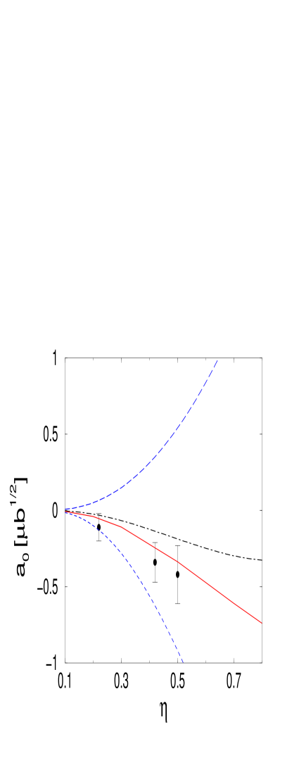
Figure 39: $a_{0}$ of $pp\to np\pi^{+}$ in chiral perturbation theory. The different lines correspond to values of the parameter related to the three–nucleon force: $\delta=1$ (long dashed line). $\delta=0$ (dot–dashed line), $\delta=-0.2$ (solid line), and $\delta=-1$ (short dashed line). Data are from Ref. [112].

It is important to extract the parameter $d$ from experiment. So far this was done only for the reaction $pp\to pn\pi^{+}$—the corresponding data is given in Ref. [112]. As was argued above, only the amplitude corresponding to the transition ${}^{1}\!S_{0}\to\,^{3}\!S_{1}p$ (called $a_{0}$) is influenced by the corresponding contact interaction. The results of the chiral perturbation theory calculations are shown in Fig. 39 for different values of the parameter $\delta$. Thus we find that the results for $a_{0}$ are indeed rather sensitive to the strength of the contact interaction. The authors of Ref. [113] claim that, with $\delta=-0.2$, the contact term gives an important contribution to $A_{y}$ in $Nd$ scattering at energies of a few MeV

It turns out that the contribution of pion rescattering is very sensitive to the regulator employed in the convolution of the production operator and the final state wave function. This scheme–dependence needs to be compensated by a counter term, namely the $NN\to NN\pi$ contact term of interest here. It is thus very important, to prove the consistency of the whole scheme, to show that the same operator strength also contributes to observables in other channels.

In Ref. [114] it was shown that the differential cross section and analysing power for the reaction $pn\to pp\pi^{-}$ for low $pp$ excitation energies is sensitive to an interference of the $s$–wave $A_{11}$ pion–production amplitude (${}^{3}\!P_{0}\to\,^{1}\!S_{0}s$) and the $p$–wave amplitudes of $A_{01}$, viz. ${}^{3}\!S_{1}\to\,^{1}\!S_{0}p$ and ${}^{3}D_{1}\to\,^{1}\!S_{0}p$. Obviously, the four–nucleon contact interaction contributes to both. Thus, once a proper chiral perturbation theory calculation is available for the $s$–wave pion production, the reaction $pn\to pp\pi^{-}$ close to the production threshold might well be the best reaction from which to extract the parameter $d$. The initial state is an isoscalar and thus the $\Delta$–nucleon intermediate state does not contribute before pion emission. Secondly, the leading $p$–wave amplitude is the one of interest, in contrast to $pp\to pn\pi^{+}$, where $p$–wave pion production is completely dominated by the transition ${}^{1}\!D_{2}\to\,^{3}\!S_{1}p$ involving production through the $\Delta$.

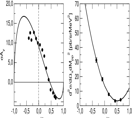
Figure 40: Analysing power and differential cross section of the $np\to pp\pi^{-}$ reaction at T_Lab = 353 MeV ($\eta=0.65$) and $E_{pp}<3$ MeV. The experimental data are from Ref. [115] and [116]. The curves are polynomial fits up to second order in the pion momenta.

The goal of the proposed COSY measurement is to provide the missing observables needed to extract the amplitudes for the transitions ${}^{3}\!S_{1}-\,^{3}\!D_{1}\to\,^{1}\!S_{0}p$ unambiguously, where the final $pp$ state is isolated by putting a tight cut on the $pp$ excitation energy $E_{pp}$. The TRIUMF data, shown in Fig. 40, are consistent with the assumption that at $T_{lab}=353$ MeV only terms up to quadratic in the outgoing pion momentum need to be kept in the expressions. This implies that, in addition to the amplitudes of interest, three additional ones have to be considered. These, which all relate to the isospin–1 initial state, correspond to ${}^{3}\!P_{0}\to\,^{1}\!S_{0}s$, ${}^{3}\!P_{2}\to\,^{1}\!S_{0}d$, and ${}^{3}\!F_{2}\to\,^{1}\!S_{0}d$.

To extract the two $p$–wave amplitudes, nine independent observables are required, of which the TRIUMF data provides five (here each angular structure is counted as an individual observable). Now, a recent measurement at Uppsala found a sizable pion $d$–wave contribution, even quite close to the production threshold [117], and these data give the values of another two observables. At least two further measurements are required and it would be preferable to measure more in order to eliminate discrete ambiguities and improve the statistical and systematic precision, especially when deuterium targets are employed. In addition to repeating some of the earlier measurements, we now consider the following possibilities for finding new observables at ANKE:
1: $A_{y}(\vec{p}p\to pp\pi^{0})$,
2: $A_{yy}(\vec{p}\vec{n}\to pp\pi^{-})$,
3: $A_{y}(\vec{p}n\to pp\pi^{-})$,
4: $A_{yy}(\vec{p}\vec{p}\to pp\pi^{0})$.

7.1.3 Experimental considerations

Simulations of the $pp\to(pp)\pi^{0}$ reaction were undertaken at a beam energy of $T_{p}=353$ MeV, which was the same as in the TRIUMF experiment [115, 116]. At this energy, proton pairs with small excitation energy ($E_{pp}<3$ MeV) can be registered in the ANKE positive side detector system. These protons typically have momenta around 400 MeV/c and for these a 2$\%$ momentum and a $0.4^{\circ}$ angular resolution were assumed in the simulation. From the acceptance of ANKE as function of the $\pi^{0}$ polar angle shown in Fig. 41, it is seen that there are no blind spots in the angular distribution.

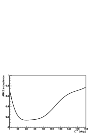
Figure 41: Predicted ANKE acceptance as a function of the $\pi^{0}$ polar angle.

The missing mass resolution is expected to be about 5.5 MeV (RMS) and this will allow one to distinguish unambiguously the pion production reaction from any background.

In Fig. 42 the resolution pion cm polar angle is shown as a function of this angle. Given that so few partial waves are expected and that both the cross section and analysing power vary smoothly with $\theta_{\pi}^{cm}$, this resolution is quite sufficient for the purpose.

In order to ensure that the final proton pair is in the ${}^{1}\!S_{0}$ state, it is important to put a tight cut on their excitation energy, to be below say 3 MeV. As shown in Fig. 43, the resolution in excitation energy is better than $0.4$ MeV at 3 MeV, though this is more vital for the cross section than the asymmetries.

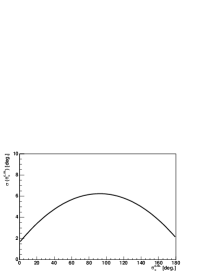
Figure 42: Predicted resolution in the pion cm polar angle.

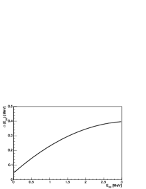
Figure 43: Predicted resolution in the $pp$ excitation energy.

The experimental conditions within the magnetic spectrometer for measuring the quasi–free $pn\to(pp)\pi^{-}$ reaction on a deuterium target are rather similar to those appertaining to the $\pi^{0}$ production. The $\pi^{-}$ does not need to be detected but the overall rate is reduced because of the acceptance of the silicon counters for the spectator proton, as described in §3.3. It must also be recognised that the Fermi momentum of the struck neutron spreads the cm energy in the initial proton–neutron system over 10’s of MeV so that some binning of the results will be required in the analysis.

It is therefore clear that both $\pi^{0}$ and $\pi^{-}$ production in the 350 MeV region can be well studied in ANKE over the full range of pion angles. The energy resolution is good enough allow one to select final proton pairs with small excitation energy. The counting rates in the case of the polarised target still have some uncertainty but, if we assume a luminosity of $10^{30}$ together with values of the $np\to pp\pi^{-}$ cross sections at 345 MeV [118], we obtain the counting rates shown in Fig. 44.

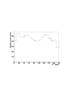
Figure 44: Predicted counting rates for the $pn\to pp\pi^{-}$ reaction at 345 MeV for a luminosity of $10^{30}$. These must be multiplied by the acceptance of the spectator counters.

These counting rates have not yet incorporated the reduction due to the acceptance of the silicon telescopes. With the extended system under discussion, this factor should be of the order of 20%. From these estimates it is clear that statistical precision should not pose a serious problem.

Test data on the $pp\to pp\pi^{0}$ reaction were taken during the same runs as for the $pd\to(pp)n$ reaction [76]. The preliminary analysis of the data at 800 MeV are shown in Fig. 45 with the same diproton selection $E_{pp}<3$ MeV [119]. It should be stressed that in this analysis only events where both tracks hit the same counter have so far been retained, thus demonstrating that the missing mass is sufficient for the clean identification of the $pp\to pp\pi^{0}$ reaction, despite the cross section being over two orders of magnitude smaller than for $pp\to d\pi^{+}$. When the tracks are observed in different counters, in addition to missing mass, we have the information about ionisation losses and the difference in time of flight. Such events will therefore be identified with even greater reliability. In addition to the well separated $\pi^{0}$ peak, there is clear evidence for $(\pi\pi)^{0}$ production, for which the threshold is at 0.073 (GeV/c²)².

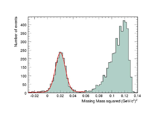
Figure 45: Preliminary data on the $pp\to ppX^{0}$ reaction in the forward direction at 800 MeV where the $pp$ excitation energy is selected to be below 3 MeV. The tracks from both protons have here been detected in the same counter.

Since data corresponding to $pd\to ppX$ were also taken, we should be able to extract also the cross sections for $pn\to(pp)\pi^{-}$. Given that there are only two spin amplitudes for either $pp\to pp\pi^{0}$ or $pn\to pp\pi^{-}$, provided that the final diproton is constrained to be in the ${}^{1}\!S_{0}$ state, measurements of the analysing powers and spin correlations are sufficient for a complete amplitude analysis.

7.2 $\vec{n}\,\vec{p}\to d\,X$

7.2.1 $\vec{n}\,\vec{p}\to d\,\pi^{0}$

It is doubtful whether a $pp\to d\pi^{+}$ reaction, taking place in the PIT, could be identified purely by detecting the fast deuteron but, as shown in Fig. 11, the $d\pi^{+}$ coincidence generally falls outside the ANKE acceptance. However, the bands corresponding to the quasi–free $\vec{n}p\to d\pi^{0}$ reaction at 585 MeV per nucleon are clearly seen in the polarised deuteron test data of Fig. 28. The ranges of cm angles covered, which are illustrated in Fig. 26, change only slowly with beam energy. Not knowing the vertex in the PIT with such high precision, the accuracy of the reconstruction will not be as good as that shown in Fig. 28 but should still be sufficient for measuring the reaction with polarised beam and target. At low energies the very extensive data base on $pp\to d\pi^{+}$ [37] would allow useful checks on the systematics of measurements with a polarised target but at high energies such experiments would add new information to the World data set.

Now the unpolarised $pn\to d\pi^{0}$ reaction has also been studied at around 556 MeV using a deuterium target at ANKE [120]. The fast deuteron was measured in the Forward Detector and the spectator proton in a prototype of the silicon telescopes described in §3.3.

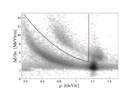
Figure 46: The normalised energy loss per centimetre for particles in the first hodoscope layer of the ANKE forward detector vs their measured momentum. Clearly visible are the upper and lower bands originating from deuterons and protons respectively. Note that the entries are shown on a logarithmic scale of greyness so that the statistics for protons are orders of magnitude greater than for deuterons. The lines indicate the cuts applied to select deuterons shown in Fig. 47

Energy losses of particles in the first plane of the scintillator hodoscope of ANKE are plotted vs their reconstructed momenta in Fig. 46. The spectrum is dominated by the proton peak around 1.17 GeV/c corresponding to small–angle deuteron break–up events. However, there are also clear proton and deuteron bands and, by imposing a momentum–dependent threshold between them, one can reduce the proton contribution significantly. Since the Landau tail from the quasi–elastic protons cannot be suppressed very effectively at high momenta, only the range below 1.15 GeV/c was selected to extract the $pn\to d\pi^{0}$ cross section, as indicated in the figure.

The experimental momentum distribution is compared in Fig. 47 to a Gaussian fit for the $d\pi^{0}$ events plus a polynomial ansatz for the background. Since the experiment was carried out very close to the two–pion threshold, the background must arise almost entirely from protons misidentified as deuterons. This is the major problem of this type of experiment.

Figure 47: Deuteron momentum distributions obtained using spectator protons with kinetic energies in the range $2.6\leq T_{\mathrm{sp}}\leq 4.4\,$MeV together with energy losses in the hodoscope for proton suppression.

A total cross section of $\sigma_{\mathrm{tot}}(pn\to d\pi^{0})=(1.62\pm 0.14)\,$mb was deduced from this experiment at an effective mean beam energy of $T_{\mathrm{beam}}=556\,$MeV. A direct measurement of this cross section with a neutron beam at this energy gave $\sigma_{\mathrm{tot}}(np\to d\pi^{0})=(1.6\pm 0.27)\,$mb [121]. This shows that, even with the modest spectator counter system, we can be more than competitive with the results obtained with neutron beams. Because the spectator proton might give more information regarding the reaction vertex, this approach looks promising for the measurement of $\vec{p}\,\vec{n}\to d\pi^{0}$ with polarised beam and target.

7.2.2 $\vec{n}\,\vec{p}\to d\,\pi\pi$

Though the importance of the coupling of the $I=1$ $NN$ and $N\Delta$ systems has been stressed earlier, the coupling to the $\Delta\Delta$ channel should be significant for the $I=0$ observables [122]. Experimental studies here necessarily involve two–pion production.

The most prominent feature of two–pion production in nuclear reactions is the so–called ABC effect, which was first detected as a sharp ($\Gamma\approx 50$ MeV/c²) $I=0$ $s$–wave enhancement in the two–pion spectrum at a mass $m_{\pi\pi}\approx 310$ MeV/c² in the reaction $pd\to\,^{3}$He$\,X^{0}$ [123]. Even sharper structure was seen in the $dd\to\,^{4}$He$\,X^{0}$ reaction, where the forward and backward (cm) peaks completely dominate the spectrum [124]. Since the positions and widths of the peak tend to change with the kinematical conditions, it was long realised that this was not a $\pi\pi$ resonance but rather some dynamical effect. The cross section and deuteron analysing powers in the $dd\to\,^{4}$He$\,X^{0}$ case [125] could all be well explained quantitatively in a model where there was independent excitation of two $\Delta(1232)$ isobars [126]. The ABC structure then arises through the $p$–wave nature of the $\Delta$ decay, where the pions tend to be emitted forward or backward. When they come out together one gets a low mass peak whereas if they emerge back–to–back there is a rather broader enhancement at maximum missing mass, which is also clearly seen in the data [124].

Of most importance theoretically is the case of $np\to d\pi\pi$ since this is likely to be linked most directly to the $\Delta\Delta$ degrees of freedom in the nuclear force. The experimental data here are of much poorer quality, having been produced through inclusive production on a deuterium target [127] or with neutron beams [128]. As a result, though the low missing mass peaks of Fig. 48a are clearly there, as is the central bump, they are a bit smeared out.

The bare double–$\Delta$ model of Fig. 48b [129], which has been refined to include residual $\Delta\Delta$ and $\Delta N$ interactions [130], gives a fair description of the experimental data at 1.88 GeV/c shown in Fig. 48a. Deviations can be ascribed in part to the effects of smearing in the incident neutron momentum. However, it should be noted that this momentum corresponds to an average excitation energy of $Q=511$ MeV, which is quite close to $2(M_{\Delta}-M_{N})\approx 586$ MeV/c². On the other hand, at $Q=363$ MeV, which is well below the $\Delta\Delta$ threshold, the cross section is much smaller and there is no sign of the ABC structure [131]. The reaction at these lower energies may be driven mainly by the Roper resonance that is excited on one of the nucleons [132].

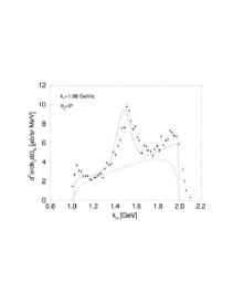
(a) Differential cross section at an average neutron momentum of 1.88 GeV/c and laboratory detection angle of 0^∘ [128]. The dashed curve represents phase space and the solid one a double–$\Delta$ estimate [130].

(b) Bare double–$\Delta$ model

Figure 48: The ABC peaks and central bump in $np\to dX$.

There are, as yet, no estimations available for the spin dependence of double–pion production in either the double–$\Delta$ or Roper models. For the excitation of a $0^{+}$ ABC in the forward direction, there are two spin–dependent amplitudes:

$$F(pn\to d\,ABC)=A\,(\mbox{\boldmath${\epsilon}$}_{pn\parallel}\mbox{\boldmath${\epsilon}$}_{d\parallel}^{\dagger}+B\,(\mbox{\boldmath${\epsilon}$}_{pn\perp}\cdot\mbox{\boldmath${\epsilon}$}_{d\perp}^{\dagger})\>,$$ (7.10)

where $\mbox{\boldmath${\epsilon}$}_{pn}$ represents the spin–1 combination of the initial $pn$ system and parallel and perpendicular are with respect to the beam direction. The magnitudes of the two amplitudes can be separated by measuring the transverse spin correlation [133]:

$$C_{NN}=\frac{|A|^{2}}{(|A|^{2}+2|B|^{2})}\>,$$ (7.11)

from which it can be seen that $C_{NN}$ can never be negative.

In the $\Delta\Delta$ model, the peak of the $pn\to d\,ABC$ cross section comes in a region where there is relatively little excitation energy with respect to $2M_{\Delta}$ [130]. The main contributions are therefore likely to be dominated by $L_{\Delta\Delta}=0$, in which case $S_{\Delta\Delta}=1$ or 3, corresponding to initial angular momenta of $0$ and $2$. However the transition from the $np$ to the $\Delta\Delta$ states depends upon which meson exchanges dominate. The ratio $|B|/|A|$ will therefore provide information on the spin dependence of the $NN\to\Delta\Delta$ potential.

7.3 The production of heavier non–strange mesons in $NN$ collisions

7.3.1 Missing–mass experiments

The ANKE spectrometer is well suited to the measurement of near–threshold production of mesons in $pp$ and, by using the silicon telescopes, $pn$ collisions. Experiments are also possible at higher energies though the phase–space coverage is then restricted. As examples of the capabilities of the spectrometer, we show in Fig. 49 missing–mass results in the $\eta/\omega$ region obtained at 2.85 and 2.95 GeV/c in $pp\to ppX$, where one proton was measured in the forward detector and the other in the positive side detector. These momenta correspond to excess energies of $Q=60$ and $Q=92$ MeV with respect to the central mass of the $\omega$–meson and over 300 MeV for the $\eta$ [134].

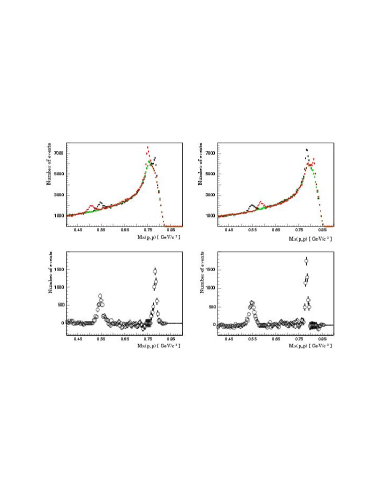
Figure 49: Missing–mass spectra (black points) in proton–proton collisions at 2.85 GeV/c (upper left panel) and 2.95 GeV/c (upper right panel). The backgrounds (green) were estimated by using the data at the other momentum, as described in the text. Once subtracted, these leave the clear $\eta$ and $\omega$ peaks shown in the lower two panels [134].

The $\omega$ missing–mass peaks at the two excess energies sit close to the maxima in the multi–pion background and so a robust treatment of this is necessary in order to extract the number of $\omega$ counts. The shape of this background is largely determined by the ANKE acceptance convoluted with a multi–pion phase space. It varies little with beam momentum provided that the curve is plotted with respect to the maximum missing mass allowed at that beam energy. More quantitatively, it was shown in the analysis of the SATURNE $pp\to pp\,\omega$ data [135] that, if the momenta of the final protons are kinematically transformed from one beam momentum below the $\omega$ threshold to another above, the background obtained in this way gives a very reliable description of the multi–pion production under the $\omega$ peak. Of course, when carrying out this procedure, the effects of the relative luminosities have to be taken into account.

This method was subsequently used to extract signals for the $pn\to d\,\omega$ reaction from quasi–free production on the deuteron, where the spectator proton was detected in a prototype silicon telescope [136].

The black points in Fig. 49 show the total missing–mass spectra at the two energies and, since below–threshold data were not available, use had to be made of the fact that in the SATURNE transformation only for the single–particle final states $X=\eta,\,\omega$ does the peak change its position, as illustrated by the red points. Taking the two data sets together, there is sufficient information to remove the unwanted single–meson peaks from the red background points to leave the smooth green points. The subtraction of the green from the black then resulted in the lower panels of Fig. 49, which shows the $\eta$ and $\omega$ peaks with very little background. This demonstrates that a model–independent approach to the treatment of multi–pion background works quite well at ANKE, at least, in the case of missing mass distributions obtained from the total acceptance. For differential distributions in centre–of–mass angle and excitation energy of the diproton, this method is more sensitive to the details of the acceptance and this is currently under investigation [134].

7.3.2 Exclusive measurements

The decays of the $\eta$ and $\omega$ mesons lead to neutral particles whose detection would require a spectrometer such as WASA [4]. However, the $\phi$ meson has an almost 50% branching ratio to $K^{+}K^{-}$, which can be detected in the ANKE system. Preliminary data on both $pp\to pp\,\phi$ and $pn\to d\,\phi$ are available where kaon pairs were measured in coincidence with fast protons and deuterons from hydrogen and deuterium targets respectively [137].

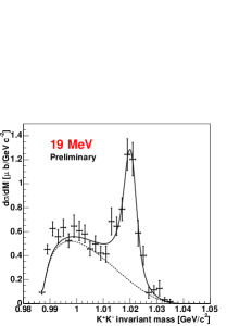
(a) Data taken at 2.65 GeV ($Q=17$ MeV)

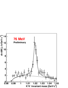
(b) Data taken at 2.83 GeV ($Q=76$ MeV)

Figure 50: $K^{+}K^{-}$ invariant mass spectra in the reaction $pp\to ppK^{+}K^{-}$. The dotted curves show four–body phase–space simulations of non–resonant $K^{+}K^{-}$ production, whereas the solid ones include also contributions from $\phi$ production.

From the $K^{+}K^{-}$ invariant mass spectra shown for the $pp$ case in Fig. 50 it is seen that the $\phi$ peak stands out clearly from a background that might have its origins mainly in the production of the much broader $a_{0}/f_{0}$ states.

The $pn\to d\phi$ reaction could be identified from $pd\to p_{s}dK^{+}K^{-}$ data, where the momentum of the spectator proton ($p_{s}$) was obtained by kinematically fitting the information from the deuteron and kaon measurements. The spectator momentum distribution shown in Fig. 51b agrees well with that predicted from the deuteron wave function. The $K^{+}K^{-}$ invariant mass spectrum of Fig. 51a shows a $\phi$ peak on a much lower background than in the $pp$ case and this difference might already contain information on the isospin dependence of $a_{0}/f_{0}$ production.

Though the beam energy was fixed at 2.65 GeV, the variation in the magnitude and direction of $\mbox{\boldmath${p}$}_{s}$, allowed one to scan the cross section in steps in excitation energy up to 80 MeV. This is completely analogous to the CELSIUS extraction of the $pn\to d\eta$ cross section where the $\eta$ decay into two photons was used to provide the spectator momentum reconstruction [138].

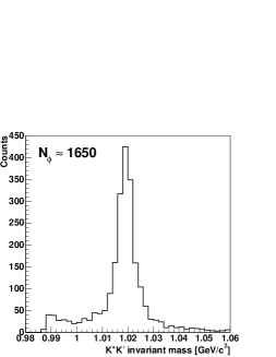
(a) $K^{+}K^{-}$ invariant mass distribution

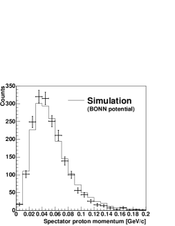
(b) Reconstructed proton spectator momentum distribution compared to a simulation using the Bonn deuteron wave function.

Figure 51: Events corresponding to the $pd\to p_{s}dK^{+}K^{-}$ reaction at a beam energy of 2.65 GeV.

Preliminary values of the $pn\to d\phi$ and $pp\to pp\phi$ total cross sections measured at ANKE are shown in Fig. 52 and compared to the energy dependence expected from phase space, viz. $\sqrt{Q}$ and $Q^{2}$ respectively. The ratio of these cross sections is much less than that observed for $\eta$ production [138], indicating that the isospin dependence is much weaker for $\phi$ than $\eta$ production.

If the $\phi$ meson were an ideal mixture containing only strange quarks then its production by hadrons containing no strangeness would be forbidden by the Okubo–Zweig–Iizuka (OZI) rule, which does not allow diagrams with disconnected quark lines [140]. Deviations from ideal mixing are small and these suggest that, under similar kinematic conditions, the ratio of single $\phi$ to $\omega$ production should be about $4.2\times 10^{-3}$. Using $\omega$ data from $pp\to pp\,\omega$ [135, 141] and $pn\to d\,\omega$ [136], it is possible to quantify deviations from the OZI rule in both the $pp$ and $pn$ channels. As seen in Fig. 52b, there is some evidence that the deviation from the OZI rule prediction increases slightly with excess energy.

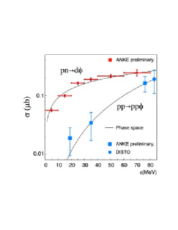
(a) Total cross section for $\phi$ production in $pp\to pp\phi$ and $pn\to d\phi$ reactions as functions of the excess energy. In addition to the ANKE measurements [137] the DISTO result is also shown [139]. The curves show the behaviour expected from phase space.

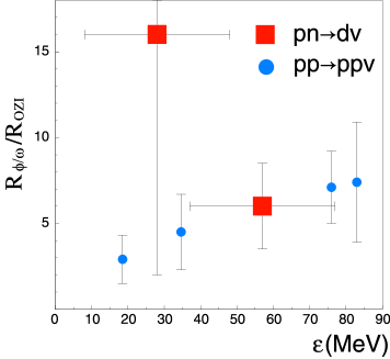
(b) The ratios of the total cross sections for $\phi$ and $\omega$-meson production in $pp$ and $pn$ collisions. The ratio is normalised using $R_{OZI}=4.2\times 10^{-3}$, which follows from the naive OZI rule.

Figure 52: Cross sections for vector meson production in nucleon-nucleon collisions.

7.3.3 Polarisation measurements

Very little is known about the spin dependence in the production of mesons heavier than the pion. The only analysing power measurement in $\vec{p}p\to pp\eta$ was carried out using the COSY11 spectrometer [142]. The signal shown in Fig. 53 is not very strong and does not constrain seriously the theoretical calculations [143, 144]. Clearly, far more detailed polarisation measurements are needed to provide clues on the underlying dynamics.

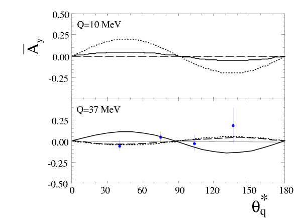
Figure 53: Proton analysing power in the reaction $\vec{p}p\to pp\eta$ as a function of the $\eta$ cm angle. The data [142] are compared to the theoretical predictions of Ref. [143] (dotted curves) and [144] (solid and broken curves).

At threshold only a single spin amplitude survives in each of the $pp\to ppX$ ($X=\eta,\,\omega,\,\eta^{\prime},\,\phi$) reactions and a similar uniqueness follows for $pn\to dX$ and the isoscalar channel in $pn\to pnX$. Under these conditions, measurements of the values of the spin correlation parameter $C_{nn}$ would serve little purpose because they are already fixed by spin–parity constraints [145, 146]. One has therefore to measure away from threshold in order to provide extra tests on the reaction dynamics. Two obvious candidates for such experiments in missing–mass mode are $\vec{p}\,\vec{d}\to p_{s}d\,\eta/\omega$, with the spectator proton measured in the silicon telescope providing the vertex determination.

There are connections between $C_{nn}$ and the spin alignment (tensor polarisation) of the produced vector meson that can be measured through the angular dependence of one of the decay products in $\omega\to\pi^{+}\pi^{-}\pi^{0}$ or $\phi\to K^{+}K^{-}$ [145, 146]. For $\phi$ production through $pp\to pp\phi$ in the forward direction at small $pp$ excitation energies the alignment determines $C_{nn}$ completely, but this is an extreme case.

7.4 Meson production in $\vec{p}\,\vec{d}\to\,^{3}\textrm{He}\,X$ reactions

Because of the double charge on the helium nucleus, the $pd\to\,^{3}\textrm{He}\,X$ reaction can often be cleanly isolated on a large background. We here describe what one might learn from measurements of $\pi$ and $\eta$ production with polarised beam and target. However, this is far from being a complete list, and it would also be interesting to study the excitation of the ABC enhancement of the two–pion spectrum [123, 147], with the spin observables being pinned down.

7.4.1 $\vec{p}\,\vec{d}\to\,^{3}\textrm{He}\,\pi^{0}$

The data on the $\vec{d}\,p\to\,^{3}\textrm{He}\,\pi^{0}$ reaction near threshold are remarkable in that for a pion cm energy of only 2.7 MeV ($p_{\pi}=27$ MeV/c) the ratio of the forward to backward pion production is about a factor of SIX [148, 28]. Since at threshold the cross section must be isotropic, this indicates the influence of enormous $p$–waves (as compared to the $s$–waves) coming in very quickly. This was quantified in a more extensive Saclay experiment that measured the deuteron analysing powers as well as the differential cross section [149]. They found that near threshold

$$\frac{\textrm{d}\sigma}{\textrm{d}\Omega}\propto(1+\alpha\eta\cos\theta)\>,$$ (7.12)

where $\theta$ is the cm angle between the incident proton and final $\pi^{0}$, $\eta=p_{\pi}/m_{\pi}$ is the pion momentum in pion mass units, and the parameter had the value $\alpha\approx 4.1$.

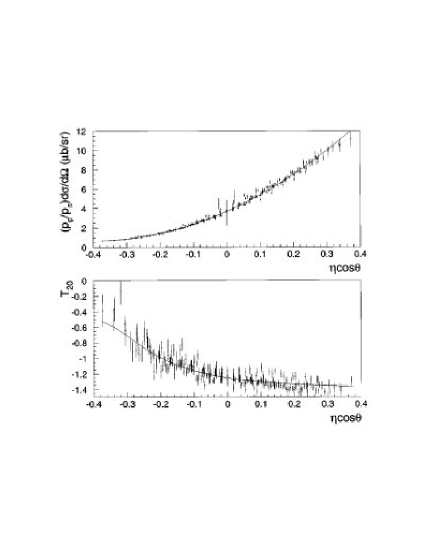
Figure 54: Averaged amplitude squared and deuteron tensor analysing power for the reaction $\vec{d}\,p\to\,^{3}\textrm{He}\,\pi^{0}$ [149]. The data at different near–threshold beam energies and angles seem to be universal functions of the parameter $\eta\cos\theta$, where $\eta$ is the pion cm momentum in pion mass units.

Even more unexpected was the observation that, after including the phase space factor, the differential cross section and deuteron tensor analysing power $t_{20}$ were functions of a single parameter $x=\eta\cos\theta$, whereas $t_{22}$ and $it_{11}$ were consistent with zero over their whole energy and angular range. These universal plots are illustrated in Fig. 54.

Now there are only two independent $pd\to\,^{3}\textrm{He}\,\pi^{0}$ amplitudes near threshold (or in the forward direction), and these may be written as [150]

$$F_{dp\rightarrow\,^{3}\!He\,\pi^{0}}=\mbox{$\sqrt{\textstyle\frac{1}{2}}$}\bar{u}_{\tau}\mbox{\boldmath${p}$}_{d}\cdot\left(A\mbox{\boldmath${\epsilon}$}+iB\mbox{\boldmath${\epsilon}$}\times\mbox{\boldmath${\sigma}$}\right)u_{p}.$$ (7.13)

Here ${\epsilon}$ is the deuteron polarisation vector, $\mbox{\boldmath${p}$}_{d}$ and $\mbox{\boldmath${p}$}_{\pi}$ the deuteron and pion centre–of–mass momenta and $u_{p}$ and $u_{\tau}$ the initial and final fermion spinors.

If only the two amplitudes $A$ and $B$ are kept, the unpolarised cm differential cross section, deuteron tensor analysing power, and vector transverse spin correlation become

$$\left(\frac{d\sigma}{d\Omega}\right) = \frac{p_{\pi}p_{d}}{3}\,(\mid A\mid^{2}+2\mid B\mid^{2})\>,$$ (7.14)

$$t_{20} = \sqrt{2}\,\frac{\left(\mid B\mid^{2}-\mid A\mid^{2}\right)}{\left(\mid A\mid^{2}+2\mid B\mid^{2}\right)}\>,$$ (7.15)

$$C_{yy} = -\frac{2Re\left(A^{*}B\right)}{\left(\mid A\mid^{2}+2\mid B\mid^{2}\right)}\>,$$ (7.16)

whereas $it_{11}$ and $t_{20}$ should both vanish.

The essence of Saclay results is that $|A|\gg|B|$, with $A$ being a steep but linear function of $\eta\cos\theta$ near threshold, the other spin amplitudes being negligible. Now, since $B$ is small, it would be better to investigate it through its interference with the $A$ amplitude and, as shown in Eq. (7.16), this is possible by the measurement of the transverse spin correlation, which should be possible with hydrogen in the PIT. The universal fit [149] suggests that $C_{yy}\,\textrm{d}\sigma/\textrm{d}\Omega$ should be a linear function of $\eta\cos\theta$.

To see why a measurement of $C_{yy}$ might be interesting, consider the description of the process within an impulse approximation picture [151, 150], which gives a simplistic but effective zeroth–order description of the experimental data [148, 28, 149]. Here pion production takes place on one nucleon in the target, with the other being a spectator, and this is reasonable near threshold (or in the forward direction) where the minimum spectator momentum is not excessive. If one neglects $D$–state effects in the deuteron and ³He, then $B$ gets a contribution only from $pp\to pp\pi^{0}$, whereas $A$ gets its largest contribution from $pn\to pn(d)\pi^{0}$ [151, 150]. Because the $\Delta$ contributes only to the latter, it is dominant over the former, and it also leads to the strong $p$–wave effects observed here [149]. Though there are potentially significant corrections to this description, including multiple scatterings and initial state distortions, it does offer the tantalising prospect of determining the relative phases of the $pp\to pp\pi^{0}$ and $pn\to pn\pi^{0}$ amplitudes near threshold, which is hard to determine in other ways.

7.4.2 $\vec{p}\,\vec{d}\to\,^{3}\textrm{He}\,\eta$

The $pd\to\,^{3}\textrm{He}\,\eta$ reaction near threshold also shows a very striking energy dependence but of a completely different nature [152, 153]. Despite the angular distribution remaining essentially isotropic, the square of the amplitude decreases by a factor of three over a few MeV in excess energy. In contrast, at higher energies, structure is seen in the angular distribution [154]. The general feeling is that the threshold behaviour is due to a very strong final state interaction between the $\eta$ and the ³He, suggesting that this system has a nearby pole in the complex momentum plane. It is not at all clear whether this corresponds to an $\eta$–nucleus quasi–bound state [155, 156, 157] or not, depending largely upon the sign of the imaginary part of the pole position. If the fsi interpretation is correct, the effect should depend only weakly upon the characteristics of the entrance channel and it is very important to verify this.

Data on $\gamma\,^{3}\textrm{He}\to\eta\,^{3}\textrm{He}$ from Mainz [158] show an even stronger energy dependence but these data are not as precise as the Saclay results and cannot be used to constrain the pole position. However, their back–to–back $\pi^{0}pX$ results indicate an anomalous behaviour just below the $\eta$ threshold, consistent with a possible decay channel of the ${}_{\eta}^{3}\textrm{He}$ nucleus, but the interpretation is not unambiguous [159].

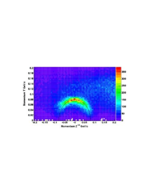
Figure 55: Transverse vs longitudinal momentum components of charged particles produced in $\vec{d}p$ collisions at $T_{d}=1811{\mbox{$\,$}}$MeV showing the momentum ellipse of events corresponding to the $\vec{d}p\to\,^{3}\textrm{He}\,\eta$ reaction.

As discussed in §7.4.1, close to threshold there are two independent $dp\to\,^{3}\textrm{He}\,\eta$ amplitudes $A$ and $B$, both corresponding the same $J^{p}=\mbox{${\textstyle\frac{1}{2}}$}^{-}$ $s$–wave in the final $\eta\,^{3}$He system. If the fsi interpretation is correct, one should see the same enhancement in both amplitudes. Unlike the pion case, the first measurement of $t_{20}$ showed that the near–threshold values of $A$ and $B$ were of similar magnitude, though the data were clearly insufficient to determine the energy dependence of the amplitudes separately [152]. This separation will be studied in detail with a polarised deuteron beam at ANKE [160] and should indicate whether the whole of the violent energy dependence is due to the final state interaction or whether the bare reaction mechanism contributes.

An even more refined test would come from the measurement of the spin correlation in the reaction since, by Eq. (7.16), this measures the interference between the two amplitudes and is sensitive to differences between the two fsi. $C_{yy}$ will, of course, be influenced by the different (though coupled) initial state interactions in the two cases, but this will be slowly varying over the few MeV over which the fsi is significant.

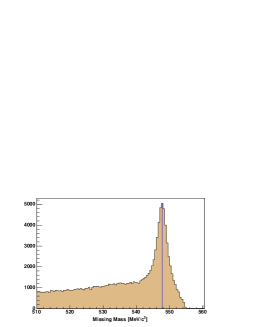
Figure 56: Missing mass spectrum for the events shown in Fig. 55. The $\eta$ peak is clearly seen sitting on a multipion background.

Data on the polarised $\vec{d}p\to\,^{3}\textrm{He}\,\eta$ reaction were taken in parallel with the deuteron charge–exchange experiment during the February 2005 beam time at an incident momentum of 3174 MeV/c ($T_{d}=1811{\mbox{$\,$}}$MeV), which is equivalent to an excess energy of $Q=8{\mbox{$\,$}}$MeV. In a preliminary analysis of these data the momentum ellipse corresponding to the reaction is seen clearly in Fig. 55. This is confirmed by the missing–mass distribution presented in Fig. 56, where a clean $\eta$ peak shows up above a physical background due to multipion production.

7.4.3 $\vec{p}\,\vec{d}\to\,^{3}\textrm{He}\,ABC$

The only measurement of the spin dependence of ABC production came as a by–product of the study of the deuteron tensor analysing power $t_{20}$ in single $\pi^{0}$ production near the forward and backward directions [28]. It should, however, be noted that the spectrometer was not optimised for such a study. The resulting data [161] show that $t_{20}$ is consistent with being constant with a value around $0.1$ for both $\theta=0^{\circ}$ and $180^{\circ}$.

In collinear kinematics, there are only two independent amplitudes

$$F=\bar{u}_{\tau}\left(A\mbox{\boldmath${\epsilon}$}_{\parallel}\mbox{\boldmath${\sigma}$}_{\parallel}+B\mbox{\boldmath${\epsilon}$}_{\perp}\cdot\mbox{\boldmath${\sigma}$}_{\perp}\right)u_{p}.$$ (7.17)

The differential cross section and the deuteron analysing power together fix the magnitudes of $A$ and $B$ and the smallness of $t_{20}$ shows that $|A|\approx|B|$. However, a measurement of the spin correlation would fix also the relative phase of $A$ and $B$ and it would be interesting to see if this is also independent of the beam energy.

8 Production of Strange Mesons and Baryons

It is well–known that the light mesons and baryons can be arranged according to the irreducible representations of the group $SU(3)$. The mass splittings within a multiplet can be well accounted for by the number of strange quarks in the baryon or meson. However, not much is known about the dynamics of systems that contain strangeness. Many phenomenological models for, e.g. hyperon–nucleon scattering [162, 163, 164, 165] use flavour $SU(3)$ to fix the meson–baryon couplings. The remaining unknowns, such as the cut–off parameters, are then fit to the data. As we discuss below, so far the existing data base for hyperon–nucleon scattering is insufficient to judge if this procedure is appropriate.

As was stressed in §7.1, effective field theories provide the bridge between the hadronic world and QCD. For systems with strangeness, there are still many open questions and up to now it is not clear if the kaon is more appropriately treated as heavy or light particle. In addition, in order to establish the counting rules it is important to know the value of the $SU(3)$ chiral condensate. For a review of this very active field of research, as well as a list of relevant references, we refer the reader to Ref. [166].

To improve further our understanding of the dynamics of systems containing strangeness, better data are needed. The insights to be gained are relevant, not only for few–body physics, but also for the formation of hypernuclei [167], and might even be of significance for the structure of neutron stars [168]). Naturally, the hyperon–nucleon scattering lengths are the quantities of interest in this context.

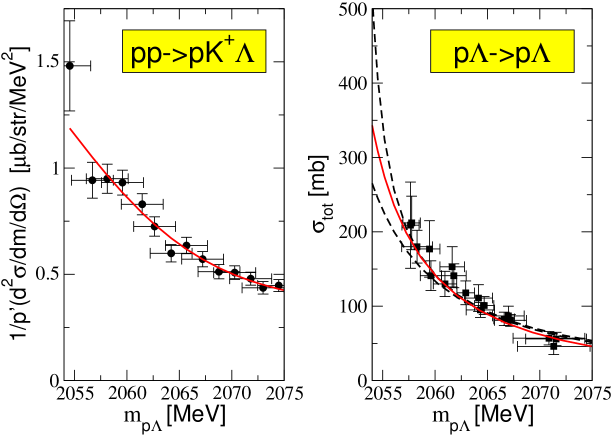
Figure 57: Comparison of the quality of available data for the reactions $pp\to K^{+}\Lambda p$ at $T_{Lab}$=2.3 GeV [169] and $\Lambda p$ elastic scattering [170, 171, 172]). In both panels the solid curve corresponds to a best fit to the data. In the right panel the dashed lines represent the spread in the energy behaviour allowed by the data, according to the analysis of Ref. [172]; analogous curves in the left panel would lie almost on top of the solid line and are therefore not shown explicitly.

In the right panel of Fig. 57 we show the World data set for elastic $\Lambda p$ scattering. In Ref. [172] a likelihood analysis, based on the elastic scattering data, was performed in order to extract the low energy $\Lambda p$ scattering parameters. The resulting contour levels, shown in Fig. 58, clearly demonstrate that the available elastic hyperon–nucleon scattering data do not significantly constrain the scattering lengths: the data allows for values of singlet and triplet scattering lengths of $(a_{s},a_{t})=(-1,2.3)$ fm as well as $(6,1)$ fm.

In subsequent work, potential models were used to extrapolate the data but even then the scattering lengths could not be pinned down accurately. For example, in Ref. [163], six different models were found that describe equally well the available data but with $S$–wave scattering lengths that range from 0.7 to 2.6 fm in the singlet channel and from 1.7 to 2.15 fm for the triplet.

There is evidence from hypernuclei that the binding energy of the spin–singlet state in ${}_{\Lambda}^{4}$He [173] is about 1 MeV stronger than for the triplet and a similar feature has been observed for ${}_{\Lambda}^{7}$Li [174]. Though the relation of this to the $\Lambda N$ interaction is not straightforward, it does suggest that the singlet force should be more attractive.

Production reactions offer a promising alternative approach. In the literature the reactions $K^{-}d\to\gamma\Lambda n$ [175], $\gamma d\to K^{+}\Lambda n$ (Ref. [176] and references therein) and $pp\to pK^{+}\Lambda$ [177] have all been suggested.

Figure 58: Values of the spin–singlet and spin–triplet scattering lengths allowed by the $\Lambda N$ elastic scattering data according to Ref. [172]. The dark shaded area denotes the 1$\sigma$ range for the parameters and the light shaded area the 2$\sigma$ range. The cross shows the best fit value ($a_{s}=1.8$ fm and $a_{t}=1.6$ fm).

ANKE can contribute to the study of the production of a variety of strange baryons in nucleon–nucleon collisions and it is likely that spin–selection will clarify some of the signals. However, we shall only discuss here two aspects of polarised $\Lambda$ production, where the Physics cases can be argued particularly clearly.

8.1 Determination of the spin–triplet $\Lambda-N$ scattering length

In Ref. [178] a method was developed that allows one to extract a scattering length directly from data from a production reaction, in terms of an integral over the invariant mass distribution, with proper kinematical factors included. A natural question that then arises is over the quality of data needed e.g. for the reaction $pp\to pK^{+}\Lambda$ in order to significantly improve our knowledge of the hyperon–nucleon scattering lengths. In Ref. [178] it was demonstrated that data of the quality of the Saclay experiment for $pp\to K^{+}X$ [169], shown in the left panel of Fig. 57 that had a mass resolution of 4 MeV, allow the extraction of a scattering length with an experimental uncertainty of only 0.2 fm. However, the actual value of the scattering length extracted from these data is not meaningful, since they represent the incoherent sum of the ${}^{3}\!S_{1}$ and the ${}^{1}\!S_{0}$ hyperon–nucleon final state with unknown relative weights.

It was shown in the previous section that the two $\Lambda N$ $S$–wave spin states can be separated in the near–threshold through by using double–polarisation measurements. However, it is not clear whether such low energy will allow one to explore the $\Lambda N$ system over a sufficiently wide range of excess energies to use the techniques of Ref. [178] to their full potential.

Now it is seen from Eq. (8.22) that the combination

$$\left(1-C_{NN}\right)\,\frac{\textrm{d}\sigma}{\textrm{d}\Omega}(pN\to K^{+}\Lambda N)$$ (8.18)

leads only to spin–triplet final states near threshold. It can be shown [114] that this is also true at higher energies provided that the $K^{+}$ is detected in the forward direction. These conditions, which are very suitable for ANKE, would allow one to investigate higher $\Lambda N$ excitation energies. As a test on the methodology, one should obtain in this way consistent results for the scattering lengths for the proton and neutron targets.

To isolate uniquely the production singlet final states through forward $K^{+}$ production far from threshold would require longitudinally polarised beam and target, neither of which is yet planned for ANKE. However, as we see below, there are further constraints in the near–threshold region.

8.2 The $NN\rightarrow NK\Lambda$ reaction near threshold

The reaction mechanism for kaon production in nucleon–nucleon collisions is still far from understood. The COSY11 [177, 179] and COSY–TOF [180, 181] collaborations have both made detailed measurements of $pp\to pK^{+}\Lambda$ and $pp\to pK^{+}\Sigma^{0}$ production near their respective thresholds, but these are insufficient to determine what the principal forces are driving the reactions. To make any progress in this respect, one needs high quality data on the spin and isospin dependence of the reactions, and ANKE is well equipped to provide these, especially in the $\Lambda$ case on which we now concentrate.

At threshold there is a total of only three amplitudes $W_{i,s/t}$ which describe the $I=1$ and $I=0$ $NN\rightarrow NK\Lambda$ reactions [182]:

$$\mathcal{M}_{1}=\left[W_{1,s}\,{\eta}_{f}^{\,\dagger}\,\mbox{\boldmath${\hat{p}}$}\cdot\mbox{\boldmath${\epsilon}$}_{i}+iW_{1,t}\,\mbox{\boldmath${\hat{p}}$}\cdot(\mbox{\boldmath${\epsilon}$}_{i}\times\mbox{\boldmath${\epsilon}$}_{f}^{\,\dagger})\right]\,\mbox{\boldmath${\chi}$}_{f}^{\,\,\dagger}\cdot\mbox{\boldmath${\chi}$}_{i}\>,$$

$$\mathcal{M}_{0}=W_{0,t}\,\mbox{\boldmath${\hat{p}}$}\cdot\mbox{\boldmath${\epsilon}$}_{f}^{\,\,\dagger}\,{\eta}_{i}\ \phi_{f}^{\,\dagger}\,\phi_{i}\>,$$ (8.19)

where ${p}$ is the incident cm beam momentum.

At least five observables are required in order to isolate these amplitudes fully (up to an overall phase). Two of these are provided by the unpolarised cross sections on proton and neutron targets, which are proportional to the intensities:

$$I(pp\!\to\!pK^{+}\Lambda)=\mbox{${\textstyle\frac{1}{4}}$}\left(\mid W_{1,s}\mid^{2}+2\mid W_{1,t}\mid^{2}\right),$$ (8.20)

$$I(pn\!\to\!nK^{+}\Lambda)=\mbox{${\textstyle\frac{1}{16}}$}\left(\mid W_{1,s}\mid^{2}+2\mid W_{1,t}\mid^{2}+\mid W_{0,t}\mid^{2}\right),$$ (8.21)

In the vicinity of the threshold, both the proton analysing power and the $\Lambda$ polarisation must vanish and only tensor combinations can be non–zero. Of these, the most easily accessible at ANKE are the transverse spin–correlation ($C_{NN}=A_{yy}$) and the spin–transfer parameters to the $\Lambda$ ($D_{NN}$), which are given by [182]

$$I(pp\!\to\!pK^{+}\Lambda)\,C_{NN}(\vec{p}\vec{p}\!\to\!pK^{+}\Lambda) = \mbox{${\textstyle\frac{1}{4}}$}\mid\!W_{1,s}\!\mid^{2}\>,$$

$$I(pn\!\to\!nK^{+}\Lambda)\,C_{NN}(\vec{p}\vec{n}\!\to\!nK^{+}\Lambda) = \mbox{${\textstyle\frac{1}{16}}$}\!\left(\mid\!W_{1,s}\!\mid^{2}\!-\!\mid\!W_{0,t}\!\mid^{2}\right)\!,$$

$$I(pp\!\to\!pK^{+}\Lambda)\,D_{NN}(\vec{p}p\!\to\!pK^{+}\vec{\Lambda}) = -\mbox{${\textstyle\frac{1}{2}}$}\textrm{Re}(W_{1,s}W_{1,t}^{*}),$$

$$I(pn\!\to\!nK^{+}\Lambda)\,D_{NN}(\vec{p}n\!\to\!nK^{+}\vec{\Lambda}) = -\mbox{${\textstyle\frac{1}{8}}$}\textrm{Re}\left\{(W_{1,s}+W_{0,t})W_{1,t}^{*}\right\},$$

$$I(pn\!\to\!nK^{+}\Lambda)\,D_{NN}(p\vec{n}\!\to\!nK^{+}\vec{\Lambda}) = -\mbox{${\textstyle\frac{1}{8}}$}\textrm{Re}\left\{(W_{1,s}-W_{0,t})W_{1,t}^{*}\right\}\>.$$ (8.22)

Measurements of the unpolarised cross section on the proton and neutron, plus the spin–correlation on the neutron, and the spin–transfer parameters in $\vec{p}p$ and $\vec{p}n$ collisions would allow one to extract the magnitudes of the three amplitudes and determine (up to two discrete ambiguities) the relative phases of $W_{1,s}$, $W_{1,t}$, and $W_{0,t}$ in a model–independent way.

The above amplitude analysis cannot, of itself, tell us whether the singlet amplitudes will be big enough to convey sufficient information to allow the study of final state interaction effects. To obtain some indication of whether this might be possible, we turn to a simple one–boson–exchange model. Neglecting distortions arising from the phase shifts in the initial $NN$ system, the amplitudes can be expressed in terms of the $\pi,\,\rho,\,\eta,\,\omega$ and the two kaon–exchange terms as [182]

$$W_{1,s} = 2\mathcal{B}_{\rho}+2\mathcal{B}_{\omega}-\mathcal{D}_{\pi}-\mathcal{D}_{\eta}+\mathcal{D}_{K}^{1}\>,$$

$$W_{1,t} = \mathcal{D}_{\pi}+\mathcal{D}_{\eta}+\mathcal{D}_{K}^{1}\>,$$

$$W_{0,t} = 6\mathcal{B}_{\rho}-2\mathcal{B}_{\omega}+3\mathcal{D}_{\pi}-\mathcal{D}_{\eta}+\mathcal{D}_{K}^{0}\,.$$ (8.23)

From this it is clear that one has no automatic right to assume that the population of $\Lambda N$ final spin states is governed purely by statistical factors.

Fäldt and Wilkin [182] speculated that $\rho$ and to a lesser extent $\pi$–exchange should provide the dominant terms. If this proves to be the case then it would mean that a large part of the $pp\to pK^{+}\Lambda$ cross section leads to spin–singlet $\Lambda p$ final states, allowing this system to be studied. However, the initial $NN$ phase shifts must be included in Eq. (8.23) before these are compared with the spin–transfer observables, which depend sensitively upon interference effects.

Such experiments cannot, of course, be carried out strictly at threshold but, from experience with $\eta$ production, the $S$–wave formulae are typically valid up to excess energies of say 20–30 MeV. Over this range in energies, the only strong variation in the $W$ amplitudes comes from the $\Lambda N$ final–state interactions, which are discussed in a more refined approach in §8.1. Though the energy limitation due to the $S$–wave selection reduces the available phase space, the different dependence of the extracted values of $\mid\!W_{1,s}\!\mid^{2}$ and $\mid\!W_{0,t}\!\mid^{2}$ on the $\Lambda N$ excitation energy will allow us to compare the effects of the spin–singlet and triplet $\Lambda-N$ scattering lengths.

It might be possible to check the spin dependence of the scattering lengths using the spin–transfer information. If, for simplicity of presentation, we neglect phases arising from the different $NN$ initial state interactions, and naïvely parameterise the $\Lambda N$ fsi purely in terms of a scattering length,

$$W_{s/t}=\frac{A_{s/t}}{(1+ika_{s/t})}$$ (8.24)

with real and slowly varying coefficients $A_{s/t}$, then

$$\frac{\left[\textrm{Re}\{W_{1,s}W_{0,t}^{*}\}\right]^{2}}{\mid\!W_{1,s}\!\mid^{2}\mid\!W_{0,t}\!\mid^{2}}=1+\frac{k^{2}(a_{s}-a_{t})^{2}}{(1+k^{2}a_{s}^{2})(1+k^{2}a_{t}^{2})}\>.$$ (8.25)

Here $k$ is the $\Lambda N$ relative momentum and the $k^{2}$ variation in Eq. (8.25) is directly a measure of the difference in the scattering lengths. When there is, in addition, a smoothly varying overall phase coming from the initial–state interactions, the above combination contains also a term linear in the scattering length difference. Though the above phenomenological description is undoubtedly crude, it does suggest strongly that there is a sensitivity to $a_{s}-a_{t}$.

8.3 Experimental considerations

The ANKE magnetic spectrometer provides a unique opportunity to investigate kaon production on a neutron target. The realisation of the ambitious programme described in the previous sections will rely on two of the advantages of the ANKE system, viz spectator particle detection, which allows one to access double polarised measurements on the neutron, and $K^{+}$ identification using time-of-flight techniques or the range–telescope structure. The $K^{+}$ production cross section is low, so that experiments will have to use the storage cell target. This then requires the full set of spectator detectors for the reconstruction of the interaction point and determination of the spectator proton momentum.

In order to be able to perform such a challenging experiment with the polarised storage cell target, the natural first step would be to undertake a sequence of the experiments with polarised beam and unpolarised deuteron target. Such a study would lead to measurements of the cross section and single polarised observables in the $pn\to nK^{+}\Lambda$ and $pp\to pK^{+}\Lambda$ channels.

Figure 59: Experimental data for the $pd\to p_{sp}K^{+}X$ reaction collected at 2.01 GeV.

In Fig. 59 are presented experimental data for the $pd\to p_{sp}K^{+}X$ reaction collected at 2.01 GeV during the August 2001 beam time. It shows that it is possible to observe coincidences between the spectator and side–detection system without imposing any limitation on the detected $K^{+}$ momentum. The spectator detector employed was a prototype, which had an acceptance only of the order of $10^{-3}$. The new spectator detection system, described in §3.3, will have much bigger acceptance and should not introduce any restrictions on the detected $K^{+}$ momentum and angle.

Figure 60: Expected count rate for the $pp\to pK^{+}\Lambda$ reaction as a function of excess energy $Q$. Stars represent conditions where only the $K^{+}$ is detected; circles correspond to the $K^{+}$ and the proton from $\Lambda$ decay being detected in coincidence.

The count rates to be expected for $K^{+}$ singles and $K^{+}p_{\Lambda}$ coincidences from the $pp\to pK^{+}\Lambda$ reaction are shown in Fig. 60. The estimations, which were made at proton beam momenta where the total cross section for the $\Lambda$ production is known [177, 180], have been made using the PLUTO event generator and AnkeRoot simulation packages [183].

The highest possible field was taken for the D2 magnet, with the point–like target being placed in the planned ABS position. A luminosity of $10^{30}$ cm^-2s^-1 was assumed in the count rate estimations. The time–of–flight start–stop combinations was excluded from the simulations because it has yet to be chosen for the new target position. However, the probability for the $K^{+}$ to decay in flight was included. Simulations which take into account the new spectator telescopes acceptance as well as the storage–cell target density distribution will be carried out in the near future.

It is important to emphasise that, even at the highest excess energy considered ($Q=85$ MeV), the momentum of the $\Lambda$ in the centre–of–mass system is at most 20% of that of the proton coming from the $\Lambda$ decay. It is therefore not necessary to measure the $\pi^{-}$ from the decay in coincidence in order to use the decay distribution to measure the $\Lambda$ polarisation in the $pn\to nK^{+}\Lambda$ reaction channel.

Up to the highest excess energy that we have considered, ANKE covers the full $K^{+}$ angular range in the CM system. The mass resolution in $n\Lambda$ system, which is also crucial for the fsi analysis described in §8.1 is expected to be better than 4–5 MeV ($\sigma$). It can be improved by operating the side chambers in the drift–chamber mode with new electronics and the installing a thinner window.

ANKE was built for the particle identification around $0^{o}$. If a longitudinally polarised beam and target would become available it is perfectly suited for the spin-singlet $\Lambda-N$ scattering length determination, since this measurement should preferably be done in the forward direction.

9 Test of Time–Reversal Invariance in Proton–Deuteron Scattering

9.1 Overview

At COSY–Jülich a novel ($P$–even, $T$–odd) null test of time–reversal invariance can be performed to an accuracy of $10^{-4}$ (Phase 1) or $10^{-6}$ (Phase 2). The parity–conserving, time–reversal–violating observable is the total cross section asymmetry $A_{y,xz}$. The measurement is planned as an internal target transmission experiment at the cooler synchrotron COSY. $A_{y,xz}$ is measured using a polarised beam and a tensor polarised deuteron target. In this experiment the COSY ring serves as an accelerator, ideal forward spectrometer, and detector.

9.2 Introduction

So far, the only link to a violation of time–reversal symmetry is given via the $CPT$–theorem and the observation of $CP$ violation in the neutral Kaon– and B–system. Although the $CP$ violation could be accommodated by a complex phase in the Kobayashi–Maskawa matrix [184] or the $\theta$ $T$–term [185] allowed by QCD, other explanations go beyond the standard model. These are, for instance, the extension of the Higgs sector [186], the superweak interaction [187], or the left–right symmetric models [188]. Such extensions lead to interactions that are not related to the observed $CP$– or $T$–violation. Since the origin of the $CP$– or $T$–violation is not clear, further experimental tests are necessary to probe the manifestation of the interaction responsible for the observed or possible new $CP$– or $T$–violating effects. In this context, more direct information is to be expected from tests involving elementary particles as compared to ones involving complex nuclei. In addition, we intend to probe time–reversal invariance with parity being conserved in contrast to experiments which test parity and time reversal invariance (TRI) simultaneously (cf. tests of the electric–dipole moments of elementary particles).

Usually $P$–even TRI tests compare two observables (cf. tests of detailed balance or $P$–$A$ tests) and this limits the experimental accuracy to about $10^{-3}-10^{-2}$ [189]. The accuracy would be increased by orders of magnitude if a true null experiment could be performed i.e. one where a non–vanishing value of a single observable proves that the symmetry involved is violated. An example of this kind is the measurement of the parity violating quantity $A_{z}$ in proton–proton scattering [190], which has been measured to some $10^{-8}$. In this context the term true stresses the concept that the intended test has to be completely independent from dynamical assumptions. Therefore, the interpretation of the result is neither restricted nor subject to final state interactions, special tensorial interactions or, Hamiltonians of a certain form. True null tests are based on the structure of the scattering matrix only, as determined by general conservation laws [191].

It has been proven [191] that there exists no true null test of TRI in a nuclear reaction with two particles in and two particles out, except for forward scattering, from which a total cross section can be measured. Based on this exception, Conzett [192] showed that a transmission experiment can be devised, which constitutes a true TRI null test. He suggested measuring the total cross–section asymmetry $A_{y,xz}$ of vector polarised spin–half particles interacting with tensor polarised spin–one particles.

We intend to study the time reversal violating (TRV) quantity $A_{y,xz}$ in a transmission experiment using an internal deuteron target in the cooler synchrotron COSY. The tensor polarised deuteron target is prepared using the polarised atomic beam target facility of the COSY experiment #5 (phase 1). Phase 2 is characterised by an improved control of systematic error contributions and the addition of a target cell to the polarised atomic beam target. The transmission losses of the circulating polarised proton beam change its lifetime. The lifetime as a function of the vector– and tensor–polarisation $P_{y}$ and $P_{xz}$ is measured by COSY’s high precision beam current transformers. Thus, for this experiment, the COSY facility is not only used as an accelerator but also as an ideal forward spectrometer and detector. The preparation of a time–reversed situation is depicted in Fig. 61.

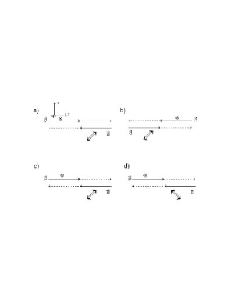
Figure 61: Pictorial demonstration that a time–reversed situation is prepared by either a proton or a deuteron spin–flip. a) The basic system is shown. b) The time–reversal operation is applied (momenta and spins are reversed and the particles are exchanged). In order to have a direct comparison between situation a) and b), two rotations $R_{y}(p)$ or $R_{x}(p)$ by $180^{\circ}$ about the $y$– or $x$–axes are applied, leading to the situations c) and d), respectively. This is allowed, since the scattering process is invariant under rotations. In the figures we have used notations whereby $\odot=$ proton spin up ($y$–direction), $\otimes=$ proton spin down, and $\Longleftrightarrow\ =$ deuteron tensor polarisation.

9.3 Experimental set–up

Since the TRV processes are of short–range nature, the long range contributions for these processes may be parameterised by the $\rho$ vector meson or $f_{1}$ axial–vector meson exchanges [192]. Using this, Beyer has shown that the most favorable momentum, where the experiment has its highest sensitivity to TRV effects, is at about 500 MeV/c [192]. Therefore, the COSY ring is presently prepared with: i) injection of polarised protons (polarisation $>0.8$) at 40 MeV, ii) stacking injection to increase the circulating proton beam, and iii) electron cooling, not only for the stacking injection, but also during the acceleration and flat–top. At the flat–top, the beam coasts for about 1 h, during which time the alignment of the target–polarisation is flipped. The beam is then decelerated and dumped and the next injection prepared, with the proton polarisation being reversed eventually from $+Y\to-Y$. Consistent results are expected for two out of the four possible combinations of the target/beam alignments/polarisations, respectively.

The resulting slopes of the decreasing circulating proton beam are measured with the high precision beam current transformers of the COSY ring. In the case that there is a TRV effect, the total cross section, and hence the slopes, would be different.

9.4 First results

A new front–end electronics and data acquisition system has been built and set up, so that the precision of the beam current transformers can be fully employed. Cooling of the beam turned out to be essential since, otherwise, the inherent emittance growth of the proton beam would cause the beam–halo to hit some aperture in the beam pipe after some minutes. This in turn would lead to a fast decrease of the beam intensity, which is not compatible with the usual exponential reduction of the current.

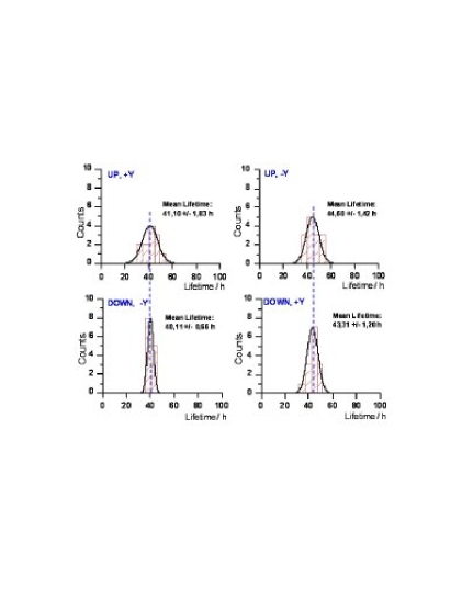
Figure 62: Results of the total asymmetry $A_{y,y}$ in $\vec{p}\,\vec{p}$ scattering at 1690 MeV/c. The agreement of the spectra for spins parallel (left) and antiparallel (right), as well as their mutual difference in lifetime, demonstrates that total cross section differences of polarised particles show up in life–time differences and that these can be measured in an internal experiment. The effect corresponds to about 3 mb [193]. UP/DOWN refers to the target polarisation, $+Y/-Y$ refers to the beam polarisation.

As a first test, the total cross–section asymmetry $A_{y,y}$ in $\vec{p}\,\vec{p}$ scattering has been measured at 1690 MeV/c (with stochastic cooling, polarisation of beam and target $>0.8$). In $\vec{p}\,\vec{d}$ scattering this quantity is the only one that through slight misalignments can fake a TRV effect. However, in contrast to the total cross–section asymmetry $A_{y,y}$ in $\vec{p}\,\vec{p}$ scattering, its value is not known. Fig. 62 shows that the novel method to measure total cross sections of polarised particles works in practice. The cross section difference in the literature [193] corresponds to a fractional lifetime difference of 6.7% compared to the COSY measurement of $8.6\pm 4.5\%$. The accuracy achieved so far is already sufficient to determine $A_{y,y}$ in $\vec{p}\,\vec{d}$ scattering, which can be accomplished by exchanging the gas supply for the target from hydrogen to deuterium.

10 Spin Rotation and Birefringence in Storage Rings

It is well known in nuclear and particle physics how to measure a total spin-dependent cross-section in, e.g. proton-proton ($pp$), proton-deuteron ($pd$), proton-nucleus ($pA$), and deuteron-nucleus ($dA$) interactions. However, measurements of the real part of the coherent elastic forward scattering amplitude $\Re[f(0)]$ poses some difficulties.

It has been shown in Refs [194, 195] (and references therein) that there is an unambiguous method which makes possible the direct measurement of the real part of the spin-dependent forward scattering amplitude by observation of proton (deuteron, or antiproton) beam spin rotation in a polarised nuclear target and by deuteron spin rotation and oscillation in an unpolarised target.

Spin rotation and oscillation experiments also allow one to carry out new experiments to study $P$– and $T$–odd interactions [194, 195].

Considering the evolution of the spin of a particle in a storage ring one should take into account several interactions. The equation for the particle spin wavefunction considering all these interactions can be written as

$$i\hbar\frac{\partial\Psi(t)}{\partial t}=\left(\hat{H}_{0}+\hat{V}_{EDM}+\hat{V}_{\vec{E}}+\hat{V}_{\vec{B}}+\hat{V}_{E}^{nucl}+\hat{V}_{{B}}^{nucl}\right)\Psi(t)$$ (10.26)

where $\Psi(t)$ is the particle spin wavefunction, $\hat{H}_{0}$ is the Hamiltonian describing the spin behavior caused by the interaction of the magnetic moment with the electromagnetic field, $\hat{V}_{EDM}=-d\left(\vec{\beta}\times\vec{B}+\vec{E}\right)\vec{S}$ describes the interaction of the particles electric dipole moment (EDM) with the electric field, $\hat{V}_{\vec{E}}=-\frac{1}{2}\hat{\alpha}_{ik}(E_{eff})_{i}(E_{eff})_{k}$ describes the interaction of the particle with the electric field due to the tensor electric polarisability, $\hat{\alpha}_{ik}$ denotes the electric tensor polarisability of the particle, $\vec{E}_{eff}=(\vec{E}+\vec{\beta}\times\vec{B})$ is the effective electric field. The latter expression can be rewritten as $\hat{V}_{\vec{E}}=\alpha_{S}E^{2}_{eff}-\alpha_{T}E^{2}_{eff}\left(\vec{S}\vec{n}_{E}\right)^{2}$, where $\vec{n}_{E}=\left.\left(\vec{E}+\vec{\beta}\times\vec{B}\right)\right/|\vec{E}+\vec{\beta}\times\vec{B}|$, and $\alpha_{S}$ and $\alpha_{T}$ are the electric scalar and tensor polarisabilities of the particle, respectively. A particle with spin $S\geq 1$ also possesses a magnetic polarisability, which is described by the magnetic polarisability tensor $\hat{\beta}_{ik}$, and the interaction of the particle with the magnetic field due to the tensor magnetic polarisability is $\hat{V}_{\vec{B}}=-\frac{1}{2}\hat{\beta}_{ik}(B_{eff})_{i}(B_{eff})_{k}$, where $(B_{eff})_{i}$ are the components of the effective magnetic field $\vec{B}_{eff}=(\vec{B}-\vec{\beta}\times\vec{E})$; $\hat{V}_{\vec{B}}$ can be expressed via $\hat{V}_{\vec{B}}=\beta_{S}B_{eff}^{2}-\beta_{T}B_{eff}^{2}\left(\vec{S}\cdot\vec{n}_{B}\right)^{2}$, where $\vec{n}_{B}=\left.\left(\vec{B}-\vec{\beta}\times\vec{E}\right)\right/\left(|\vec{B}-\vec{\beta}\times\vec{E}|\right)$, and $\beta_{S}$ and $\beta_{T}$ are the scalar and tensor magnetic polarisabilities of the particle, respectively. $\hat{V}_{{B}}^{nucl}$ describes the effective potential energy of the interaction with the nuclear pseudomagnetic field of the target [194, 195], and $\hat{V}_{E}^{nucl}$ denotes the effective potential energy of the interaction with the nuclear pseudoelectric field of the target [194, 195]. It should be emphasised that $\hat{V}_{{B}}^{nucl}$ and $\hat{V}_{E}^{nucl}$ include contributions from strong interactions as well as those caused by weak interactions, violating $P$ and $T$ invariance.

Let us consider particles moving in a storage ring with low residual gas pressure ($10^{-10}$ Torr) and without other targets inside the storage ring. In this case we can omit the effects caused by the interactions $\hat{V}_{{B}}^{nucl}$ and $\hat{V}_{E}^{nucl}$ altogether. Let us further consider a particle with $S=1$ (for example, deuteron) moving in such a ring. According to the above analysis, the spin of such a particle can not be described by the BMT–equation. The equations for the particle spin motion, including contributions from the tensor electric polarisability, were obtained in Refs. [194, 195]. Considering that the deuteron possesses also a tensor magnetic polarisability, after adding the terms caused by this interaction to the equations obtained in Refs. [194, 195], we finally obtain

$$\frac{d\vec{P}}{dt}=\frac{e}{mc}\left[\vec{P}\times\left\{\left(a+\frac{1}{\gamma}\right)\vec{B}-a\frac{\gamma}{\gamma+1}\left(\vec{\beta}\cdot\vec{B}\right)\vec{\beta}-\left(\frac{g}{2}-\frac{\gamma}{\gamma+1}\right)\vec{\beta}\times\vec{E}\right\}\right]$$

$$+\frac{d}{\hbar}\left[\vec{P}\times\left({\vec{E}}+\vec{\beta}\times\vec{B}\right)\right]-\frac{2}{3}\frac{\alpha_{T}E^{2}_{eff}}{\hbar}[\vec{n}_{E}\times\vec{n}_{E}^{\prime}]-\frac{2}{3}\frac{\beta_{T}B^{2}_{eff}}{\hbar}[\vec{n}_{B}\times\vec{n}_{B}^{\prime}],$$ (10.27)

$$\frac{dP_{ik}}{dt}=-\left(\varepsilon_{jkr}P_{ij}\Omega_{r}+\varepsilon_{jir}P_{kj}\Omega_{r}\right)-\frac{3}{2}\frac{\alpha_{T}E^{2}_{eff}}{\hbar}\left([\vec{n}_{E}\times\vec{P}]_{i}n_{E,\,k}+n_{E,\,i}[\vec{n}_{E}\times\vec{P}]_{k}\right)$$

$$-\frac{3}{2}\frac{\beta_{T}B^{2}_{eff}}{\hbar}\left([\vec{n}_{B}\times\vec{P}]_{i}n_{B,\,k}+n_{B,\,i}[\vec{n}_{B}\times\vec{P}]_{k}\right),$$ (10.28)

where $m$ is the particle mass, $e$ is the charge, $\vec{P}$ is the spin polarisation vector, $P_{xx}+P_{yy}+P_{zz}=0$, $\gamma$ is the Lorentz-factor, $\vec{\beta}=\vec{v}/c$, $\vec{v}$ is the particle velocity, $a=(g-2)/2$, $g$ is the gyromagnetic ratio, $\vec{E}$ and $\vec{B}$ are the electric and magnetic fields at the position of the particle, $\vec{E}_{eff}=(\vec{E}+\vec{\beta}\times\vec{B})$, $\vec{B}_{eff}=(\vec{B}-\vec{\beta}\times\vec{E})$, $\vec{n}=\vec{k}/k$, $\vec{n}_{E}=(\vec{E}+\vec{\beta}\times\vec{B})/|\vec{E}+\vec{\beta}\times\vec{B}|$, $\vec{n}_{B}=(\vec{B}-\vec{\beta}\times\vec{E})/|\vec{B}-\vec{\beta}\times\vec{E}|$, $n_{i}^{\prime}=P_{ik}n_{k}$, $n_{E,\,i}^{\prime}=P_{ik}n_{E,\,k}$, $n_{Bi}^{\prime}=P_{il}n_{Bl}=P_{i3}$. The components of the vector $\vec{\Omega}(d)$ are given by $\Omega_{r}(d)$ (the indices $r=1,2,3$ correspond to $x,y,z$, respectively),

$$\vec{\Omega}(d) = \frac{e}{mc}\left\{\left(a+\frac{1}{\gamma}\right)\vec{B}-a\frac{\gamma}{\gamma+1}\left(\vec{\beta}\cdot\vec{B}\right)\vec{\beta}-\left(\frac{g}{2}-\frac{\gamma}{\gamma+1}\right)\vec{\beta}\times\vec{E}\right\}$$ (10.29)

$$+\frac{d}{\hbar}\left({\vec{E}}+\vec{\beta}\times\vec{B}\right).$$

From Eq. (10.28) it follows that the magnetic polarisability leads to spin rotation with two frequencies $\omega_{1}$ and $\omega_{2}$ instead of $\Omega$ and, therefore, experiments beating with the frequency $\Delta\omega=\omega_{1}-\omega_{2}=2\sqrt{\Omega_{T}^{\mu}\Omega_{T}^{\prime\mu}}=\beta_{T}B_{eff}^{2}/\hbar$. According to the evaluation in Refs. [194, 195], the tensor magnetic polarisability $\beta_{T}\sim 2\times 10^{-40}$, therefore for the beating frequency one obtains $\Delta\omega\sim 10^{-5}$ in a field of $B\sim 10^{4}$ gauss. The measurement of the frequency of this beating makes possible the determination of the tensor magnetic polarisability of the deuteron (nuclei). Thus, due to the presence of the tensor magnetic polarisability, the horizontal component of the spin rotates around $\vec{B}$ with two frequencies $\omega_{1},~{}\omega_{2}$ instead of the expected rotation with the frequency $\Omega$. The resulting motion of the spin is beating: $P_{1}(t)\sim\cos\Omega t\sin\Delta\omega t$. This is the reason for the component $P_{3}$, caused by the EDM, to exhibit a similar beating.

Another class of experiments deals with the use of polarised targets. One should recall that the density of a polarised gas target is substantially lower than the one of an unpolarised target, the anticipated density of the polarised target of ANKE, described in §3.4, is about $d_{t}=10^{14}$ cm^-2. When a particle (proton, antiproton, deuteron …) propagates through a nuclear polarised target, precession of the particle spin occurs In a polarised target the particles can be characterised by two refraction indices, $N_{\uparrow\uparrow}$ for particles with spin parallel to the target polarisation vector, and $N_{\uparrow\downarrow}$ for particles with the opposite spin orientation $N_{\uparrow\uparrow}\neq N_{\uparrow\downarrow}$. According to [194, 195], in the target with polarised nuclei, there is a nuclear pseudomagnetic field and the interaction of an incident particle with this field leads to spin rotation. The experiments with slow neutrons proved the existence of this effect [194, 195].

The effective potential energy of a particle in a pseudomagnetic nuclear field $\vec{G}$ of matter can be written as:

$$\hat{V}_{B}^{nucl}=-\vec{\mu}\vec{G},$$ (10.30)

where $\vec{\mu}$ is the magnetic moment of the particle and $\vec{G}$ can be expressed as [194, 195] $\vec{G}=\vec{G}_{s}+\vec{G}_{w}$, where

$$\vec{G}_{s}=\frac{2\pi\hbar^{2}}{\mu m}\rho[A_{1}\langle\vec{J}\rangle+A_{2}\vec{n}(\vec{n}\cdot\langle\vec{J}\rangle)+...],$$ (10.31)

$$\vec{G}_{w}=\frac{2\pi\hbar^{2}}{\mu m}\rho[b\vec{n}+b_{1}[\langle\vec{J}\rangle\times\vec{n}]+b_{2}\vec{n}_{1}+b_{3}\vec{n}(\vec{n}\cdot\vec{n}_{1})+b_{5}[\vec{n}\times\vec{n}_{1}]+...].$$ (10.32)

Here $\vec{n}=\vec{v}/v$, $\vec{J}$ is the nuclear spin, $\langle\vec{J}\rangle=\textrm{Sp}\left\{\rho_{nucl}\vec{J}\right\}$ is the average value of the nuclear spin, $\vec{n}_{1}$ are the components $n_{1j}=\langle Q_{ij}\rangle n_{j}$, where $\langle Q_{ij}\rangle=\textrm{Sp}\left\{\rho_{nucl}Q_{ij}\right\}$ is the polarisation tensor.

It is easy to see that the interaction, described by Eq. 10.30) looks like the interaction of a magnetic moment with a magnetic field, thus the field $\vec{G}$ contributes to the change of the particle polarisation similar to the one of a magnetic field. It should be mentioned that $\hat{V}_{B}^{nucl}$ contains both a real part, which is responsible for spin rotation, and an imaginary part, which contributes to the spin dichroism (beam absorption depending on the relative spin orientation). A detailed analysis of the effects caused by the nuclear pseudoelectric field is described in Ref. [194].

The interaction with the field $\vec{G}=\vec{G}_{s}+\vec{G}_{w}$ contains two terms: $\vec{G}_{s}$ corresponds to the strong interaction, which is $T$, $P$–even, while $\vec{G}_{w}$ describes spin rotation by the weak interaction, which has contributions from both $T$, $P$–odd (the term containing the constant $b_{1}$) and $T$–odd, $P$–even (the term containing the constant $b_{5}$) interactions. If either the vector or the tensor polarisation of the target rotates, the effects provided by $\vec{G}_{s}$ and $\vec{G}_{w}$ vary periodically as a function of time, i.e. Eq. (10.26) can be written as

$$i\hbar\frac{\partial\Psi(t)}{\partial t}=\left(\hat{H}_{0}+\hat{V}_{EDM}+\hat{V}_{\vec{E}}+\hat{V}_{\vec{B}}+\hat{V}_{E}^{nucl}(t)+\hat{V}_{{B}}^{nucl}(t)\right)\Psi(t).$$ (10.33)

This equation coincides with the well-known equation for a paramagnetic resonance. Thus, in a strong magnetic field, orthogonal to the weak nuclear pseudomagnetic field $\vec{B}\perp\vec{G}$, $\vec{G}$ either rotates or oscillates with the frequency corresponding to the splitting caused by $\vec{B}$, a resonance occurs and this leads to the conversion of horizontal spin components to vertical ones with the frequency determined by the spin precession frequency in the field $\vec{G}$ [195]. Thus, one can measure all the constants contained in $\vec{G}_{s}$ and $\vec{G}_{w}$: $A_{i}$ yields the spin-dependent part of the elastic coherent forward scattering amplitude of proton (deuteron, or antiproton); the amplitudes $b_{i}$ provide a measurement of the constants of $T$– and $P$–odd interactions.

The $T$–odd nucleon-nucleon interaction of protons (or antiprotons) and deuterons with polarised nuclei is described by $V_{P,T}\sim\vec{S}\cdot\left(\vec{p}_{N}\times\vec{n}\right)$, where $\vec{P}_{N}(t)$ is the polarisation vector of target. The interaction $V_{P,T}$ leads to the spin rotation around an axis given by the unit vector $\vec{n}_{T}$, parallel to $\left[\vec{P}_{N}(t)\times\vec{n}\right]$. Spin dichroism also appears with respect to this vector $\vec{n}_{T}$, i.e. a proton (deuteron) beam with spin parallel to $\vec{n}_{T}$ exhibits different absorption cross-sections depending on the spin direction.

$P$–even, $T$–odd spin rotation, oscillation and dichroism of deuterons (nuclei with $S\geq 1$) caused by the interactions of $V_{T}\sim\vec{S}\cdot(\vec{P}_{N}(t)\times\vec{n})(\vec{S}\cdot\vec{n})$ could be observed [194]; $P$–even, $T$–odd spin rotation and dichroism for a proton, deuteron (or more generally for a nucleus with spin $S\geq 1/2$) $V^{\prime}_{T}\sim b_{5}[\vec{n}\times\vec{n}_{1}(t)]$ could be observed [194, 195] in paramagnetic resonance conditions as well.

The observation of spin rotation and birefringence of particles stored in a ring provides the opportunity to measure the real part of the coherent elastic zero-angle scattering amplitude, as well as tensor electric and magnetic polarisabilities. The same information could be obtained also from particles and nuclei in a storage ring by the paramagnetic resonance method, induced by time varying nuclear pseudoelectric and pseudomagnetic fields.

11 Preparatory Work for the FAIR Project

11.1 The PAX proposal at FAIR

The PAX Collaboration is proposing a programme of spin experiments with intense beams of polarised antiprotons at FAIR. A practical and viable scheme to reach polarisations of the stored antiprotons at HESR–FAIR of about 30% has been presented [196]. The above performance is expected based on the electron–to–proton spin transfer interpretation [7, 8] of the FILTEX experiment [6]; such an approach is routinely used at Jefferson Laboratory for the separation of electromagnetic form factors [197].

The PAX Technical Proposal was submitted in January 2004. The physics programme was reviewed by the QCD Programme Advisory Committee (QCD–PAC) in June 2004 [198]. Following the QCD–PAC report and the recommendation of the Chair of the Committee on Scientific and Technological Issues (STI) and the FAIR project coordinator [198], the PAX collaboration has optimised the technique to achieve a sizable antiproton polarisation. The studies are contained in the recently submitted Technical Proposal [198]. The goal of achieving the highest possible figure of merit requires that the antiprotons be polarised in a dedicated low–energy ring. The transfer of polarised low–energy antiprotons into the HESR ring would then require pre–acceleration to about 1.5 GeV/c in a dedicated booster ring (CSR). The incorporation of this booster ring into the HESR complex would, quite naturally, open up the possibility of building an asymmetric antiproton–proton collider.

The main features of the accelerator setup, shown in Fig. 63, are:

1. An Antiproton Polariser Ring (APR), built inside the HESR area, having the crucial goal of polarising antiprotons at kinetic energies around $50$ MeV ($p_{\bar{p}}\approx 300$ MeV/c). These would subsequently be accelerated and injected into the other rings.

2. A second Cooler Synchrotron Ring (CSR) in which protons or antiprotons with momenta up to 3.5 GeV/c could be stored. This ring, whose parameters would be rather similar to those of COSY, should have a straight section running parallel to the experimental straight section of HESR, where a PAX detector could be installed.

3. By deflecting the HESR beam into the straight section of the CSR, both collider and fixed–target modes become feasible.

It is worthwhile stressing that, through the employment of the CSR, a second interaction point is effectively formed that has a minimum interference with PANDA. The proposed solution opens the possibility of running simultaneously two different experiments.

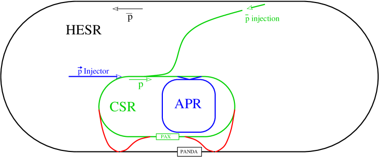
Figure 63: The proposed accelerator setup at the HESR (black), with the equipment to be used by the PAX collaboration in Phase–I: CSR (green), APR, beam transfer lines and polarised proton injector (all blue). In Phase–II, by adding two transfer lines (red), an asymmetric collider is set up. It should be noted that, in this phase, fixed target operation at PAX is also possible. (The figure is drawn to scale.)

11.2 Preparatory phase

The objectives arising from the PAX proposal for the immediate future (3–4 years) concern mainly the polarisation buildup process through which polarised antiprotons will be produced. The PAX collaboration suggests carrying out spin–filtering experiments in storage rings to achieve a better understanding of these processes in general. Furthermore, for antiprotons, the experimental basis for polarisation buildup in a stored beam is practically non–existent. Therefore, it is of highest priority for PAX to perform spin–filtering experiments using stored antiprotons, e.g. at the AD of CERN. Once the experimental data base is available, the final design of the APR can be targeted. The physics of the buildup of polarisation in a storage ring involves a number of features absent in conventional scattering experiments, especially the into–the–beam scattering of target particles, which have to be well understood before one embarks on polarising antiprotons. A few simple spin–filtering experiment carried out at COSY, would certainly enhance substantially our understanding of these processes. The PAX proposal calls eventually for an asymmetric antiproton–proton collider at the HESR. To this end, machine studies using state–of–the–art simulation tools (e.g. BETACOOL) and in depth analyses of the phase space cooling processes, intrabeam scattering effects and beam–beam interactions have to be carried out. The goal of these studies is to optimise the collider and fixed target scenarios of the PAX experiment with respect to luminosity. This naturally involves also machine studies for the dedicated Antiproton Polariser Ring (APR), which is at the core of the PAX proposal.

11.3 Spin Filtering Experiments with protons at COSY and with antiprotons at the CERN AD

Central to the PAX proposal is spin filtering of stored antiprotons by multiple passage through an internal polarised gas target. The feasibility of the technique has been convincingly demonstrated in the FILTEX experiment at TSR [6]: for 23 MeV stored protons, a transverse polarisation rate of $\textrm{d}P/\textrm{d}t=0.0124\pm 0.0006$ per hour has been reached with an internal polarised atomic hydrogen target of areal density $6\times 10^{13}$ atoms/cm². In view of the fundamental importance of spin filtering for the PAX experiment, experiments at COSY would provide the necessary data to test our present understanding of spin–filtering processes in storage rings. However, since for PAX the design of a dedicated APR is foreseen, it is crucial that such experiments be performed eventually with antiprotons at a suitable antiproton storage ring, e.g. at the CERN AD. For a proton impinging on a polarised hydrogen gas target, the spin–dependent interaction leading to the buildup of polarisation in the beam is well known; recent investigations [199] have, however, shown that an unambiguous quantitative understanding and interpretation of the FILTEX result [6] may not yet be available. In addition, there are no experimental data available on the spin correlations, or more generally, on any of the two–spin observables in antiproton–proton scattering. The final goal is to provide the experimental data base of antiproton–proton interactions that is necessary to define the optimum working parameters of the dedicated APR, suggested for FAIR. Ultimately, these measurements are needed in order to arrive at the final design parameters for the APR. The new data will, moreover, provide new insight into the $\bar{p}p$ physics more generally.

11.4 Design and construction of the Antiproton Polariser Ring

Tuning and commissioning of the APR will require a beam of polarised protons. Such a beam and a hall, including the necessary infrastructure, are available at COSY. This makes the Institut für Kernphysik of the Forschungszentrum Jülich the ideally suited site for the design, construction and testing of the APR. A floor plan of the polariser ring is shown in Fig. 64. For more details, see Ref. [198]

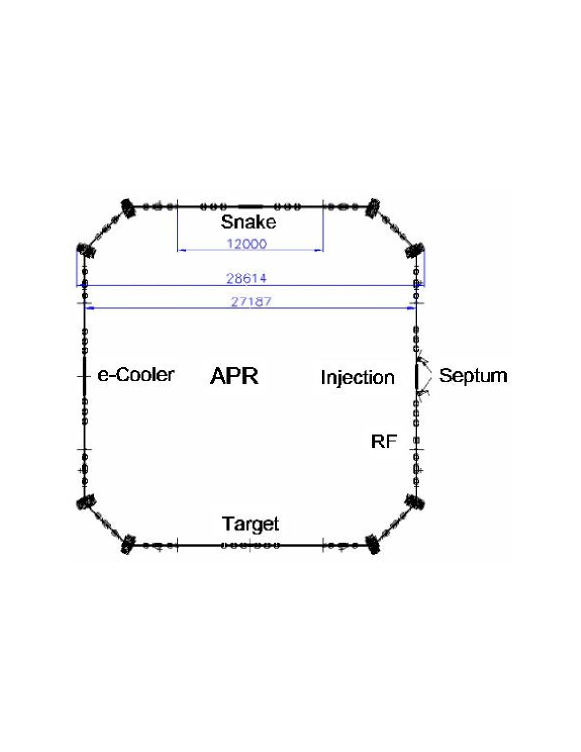
Figure 64: Floor plan of the APR lattice.

The technical feasibility of the polarisation transfer method was verified in the FILTEX experiment at TSR–Heidelberg in 1992 with a 23 MeV proton beam [6]. As mentioned above, a pre–APR test can be performed at COSY by verifying $\sigma_{EM_{\perp}}$ at 40, 70 and 100 MeV, using the polarised internal target at the ANKE interaction point. The measurement can be performed by injecting pure states $\left|1\right>$ or $\left|3\right>$ in a weak transverse target guide field (10 G). Under these conditions the electron target polarisation $Q_{e}$ is equal to the proton target polarisation $Q_{p}$. The latter can be measured through $pp$ elastic scattering with the help of the ANKE silicon telescope system described in §3.3 [200].

11.5 Development of polarised sources

The polarisation mechanism relies on an having an efficient, high–intensity, source of polarised hydrogen atoms. Most of the World–expertise on polarised sources is already present within the PAX collaboration and a programme for the development of a new generation of high–intensity atomic beam sources has to be started during the preparatory phase of the PAX experiment. The COSY experience in polarised sources and polarised beams will be crucial in this development.

11.6 Staging of the PAX experiment and the role of COSY

The final goal of the PAX collaboration is a polarised proton–antiproton asymmetric collider, in which 3.5 GeV/c polarised protons will collide head–on with polarised antiprotons with momenta up to 15 GeV/c. However, the collaboration proposes an approach composed of different stages, during which the major milestones of the project can be tested and optimised.

11.7 Phase–I: transfer of APR and CSR to FAIR

APR and CSR will be placed inside the HESR. The straight sections of CSR and HESR will be parallel, allowing an additional interaction point, independent of that of PANDA, to be formed.

A beam of unpolarised or polarised antiprotons, with momenta up to 3.5 GeV/c, will be available in the CSR ring. Collisions with a polarised hydrogen target in the PAX detector can then be studied. This first phase, which is independent of the HESR performance, will allow for the first time the measurement of the time–like proton form factors in single– and double–polarised reactions from close to threshold up to 3.5 GeV/c. It will be possible to determine several (single and double) spin asymmetries in the elastic $p\bar{p}\to p\bar{p}$ scattering. By detecting back–scattered antiprotons, one can also explore the hard scattering regions of large $t$. (Reaching the same region of $t$ in proton–proton scattering requires twice as high an energy.)

11.8 Phase–II: HESR modifications to the collider mode or to the polarised internal target

A chicane for CSR and HESR would have to be built to bring the proton beam of the CSR and the antiproton beam of the HESR to a collision point at the PAX detector. This phase will allow the first ever direct measurement of the quark transversity distribution $h_{1}$, by studying the double transverse spin asymmetry $A_{TT}$ in the Drell–Yan processes $p^{\uparrow}\bar{p}^{\uparrow}\rightarrow e^{+}e^{-}X$ as a function of Bjorken $x$ and $Q^{2}$ (= $M^{2}$). Two possible scenarios might be foreseen to perform this measurement.

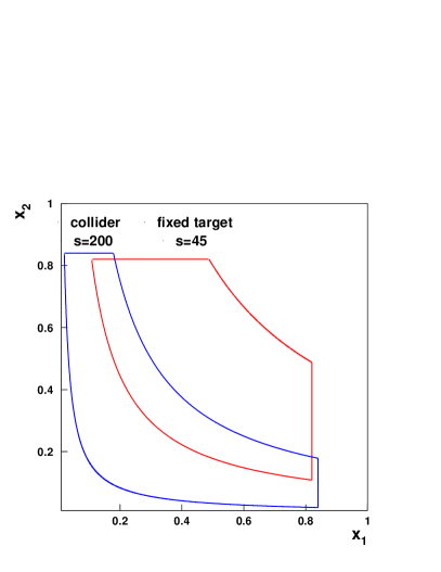
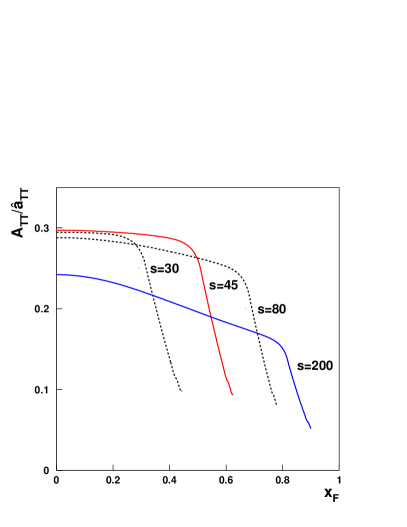
Figure 65: Left: The kinematic region covered by the $h_{1}$ measurement at PAX in phase II. In the asymmetric collider scenario (blue), antiprotons of 15 GeV/c impinge on protons of 3.5 GeV/c at cm energies of $\sqrt{s}\sim\sqrt{200}$ GeV and $Q^{2}>4$ GeV². The fixed target case (red) represents antiprotons of 22 GeV/c colliding with a fixed polarised target ($\sqrt{s}\sim\sqrt{45}$ GeV). Right: The expected asymmetry as a function of Feynman $x_{F}$ for different values of $s$ and $Q^{2}=16$ GeV².

• A beam of polarised antiprotons from 1.5 GeV/c up to 15 GeV/c, circulating in the HESR, collides with a beam of 3.5 GeV/c polarised protons circulating in the CSR. This scenario requires one to demonstrate that a suitable luminosity is reachable. Deflection of the HESR beam to the PAX detector in the CSR is necessary (see Fig. 63). By properly varying the energy of the two colliding beams, this setup would allow a measurement of the transversity distribution $h_{1}$ in the valence region of $0.1<x<0.8$ with the corresponding $Q^{2}$ in the range $4<Q^{2}<100$ GeV² (see Fig. 65). As shown in Fig. 65, the double transverse spin asymmetry ($A_{TT}$) in Drell–Yan processes with both transversely polarised beam and target is predicted to be greater than 0.2 in the full kinematic range [201, 202].

  $$A_{TT}\equiv\frac{d\sigma^{\uparrow\uparrow}-d\sigma^{\uparrow\downarrow}}{d\sigma^{\uparrow\uparrow}+d\sigma^{\uparrow\downarrow}}=\hat{a}_{TT}\>\frac{\sum_{q}e_{q}^{2}\,h_{1}^{q}(x_{1},M^{2})\,h_{1}^{\bar{q}}(x_{2},M^{2})}{\sum_{q}e_{q}^{2}\,q(x_{1},M^{2})\,\bar{q}(x_{2},M^{2})}\>,$$ (11.34)

  where $q=u,\bar{u},d,\bar{d},...$, $M$ is the invariant mass of the lepton pair, and $\hat{a}_{TT}$ is the double spin asymmetry of the QED elementary process, $q\bar{q}\to\ell^{+}\ell^{-}$,

  $$\hat{a}_{TT}=\frac{\sin^{2}\theta}{1+\cos^{2}\theta}\cos 2\phi\,,$$ (11.35)

  with $\theta$ the polar angle of the lepton in the $l^{+}l^{-}$ rest frame and $\phi$ the azimuthal angle with respect to the proton polarisation.

  Such an experiment for $h_{1}$ can be considered as the analogue of polarised deep inelastic scattering for the helicity distribution $\Delta q$. The kinematical coverage in $(x,Q^{2})$ will in fact be similar to that of the HERMES experiment [203].

• Should the desired luminosity for the collider not be reachable, a fixed target experiment can be performed. A beam of 22 GeV/c (or 15 GeV/c) polarised antiprotons circulating in the HESR, can be used to collide on a polarised internal hydrogen target. This scenario also requires the deflection of the HESR beam to the PAX detector in the CSR (see Fig. 63).

12 Time Schedules

12.1 General remarks

At present, we consider that the measurements within our spin programme should take place during the four years 2006 – 2009. We assume that during this period COSY is fully operational, providing beams from its polarised ion source, and that the ANKE polarised internal target, together with the ANKE spectrometer, are also in operation. However, the time schedule for the spin–physics programme ANKE@COSY will, of course, depend to some extent on the planning and progress for the realisation of the FAIR project.

There are currently eight PhD students (D. Chiladze, K. Grigoriev, D. Gussev, A. Mussgiller, V. Leontiev, T. Mersmann, T. Rausmann, and Yu. Valdau) working on spin–physics subjects within the framework of the ANKE collaboration. Their projects involve Monte–Carlo simulations for the different experiments as well as data analysis of experiments with polarised deuteron and proton beams. Recent data taken with the (unpolarised) storage cell target, which will provide a test for the upcoming double–polarised experiments, are also in the course of analysis. The strong involvement of members of the theory group in Jülich, as well as of external experts, provides an excellent theoretical support of the spin–physics programme at ANKE.

12.2 Submissions and requests

• April 2005 – elements of the spin document included in the submission to the POF evaluation committee were favourably received [204].

• October 2005 – presentation of the full document to the COSY PAC.

• Spring 2006 – beam–time request for $np$ double–polarised experiment.

12.3 Timelines

As described in this document, the spin–physics programme can be broadly grouped into four categories, addressing the following subjects:
1. Proton–neutron spin physics,
2. Non–strange meson production,
3. Production of strange mesons and baryons,
4. Preparatory work for the FAIR project.

The following time schedule is anticipated for the delivery of this programme:

6/2005	—	Installation of the PIT at the ANKE target position
until 6/2006	—	Commissioning of the PIT
7/2006	—	First double–polarised $np$ experiments
2007	—	Data taking with ANKE for item 1 ($\approx 3$ months)
2008	—	Data taking with ANKE for item 2 ($\approx 3$ months)
2009	—	Data taking with ANKE for item 3 ($\approx 3$ months)
2007–11	—	Data analysis & publication of results

A list of some of the possible experiments that will be carried out in parallel is presented in Table 5. The last item (4), preparations for FAIR, mainly addresses the design, building and commissioning of the Antiproton Polariser Ring, for which the time estimates are:

2006–2007	—	APR machine design
		Preparation of “ready–to–be–built” documents
		Development of a new generation of high–intensity ABS for the APR
2008–9	—	Construction of APR at IKP
2010–2011	—	Commissioning of APR
$>2012$	—	Transfer of APR and CSR to HESR

Table 5: Table of experiments that will be done simultaneously.

Phase I: Polarised deuteron beam & polarised hydrogen storage-cell target $(dp)$;
Energy range: $1.2<T_{d}<2.3$ GeV;
Instrumentation: ANKE, silicon telescopes, polarised storage-cell target.
Methodical advantage: High intensity polarised deuteron beam, high count rate, clean identification of many two-body reactions, polarimetry of target can be done without Lamb-shift polarimetry, polarimetry standards are already achieved including polarisation export technique, preparation of the polarised hydrogen target relatively easy.
Reactions:
$dp\rightarrow(2p)n$ small momentum transfer charge-exchange
$dp\rightarrow(2p)\Delta^{0}$ at minimum momentum transfer
$dp\rightarrow dp$ small angle scattering
$dp\rightarrow dp$ large angle scattering
$dp\rightarrow(2p)n$ large momentum transfer charge-exchange
$dp\rightarrow\,^{3}\textrm{He}\,\pi^{0}$
$dp\rightarrow\,^{3}\textrm{He}\,\eta$
$np\rightarrow d\pi^{0}$ quasi-free
$np\rightarrow dX(\pi\pi)$
$pp\rightarrow pp$ quasi-free
Phase II: Polarised proton beam & Polarised deuteron storage-cell target $(pd)$;
Energy range $T_{p}$ = 1.0 GeV up to 3.0 GeV;
Instrumentation: ANKE, silicon telescopes, polarised storage-cell target, Lamb-shift polarimeter.
Methodical aspects: need good adjustment of the trigger conditions.
Reactions:
$pd\rightarrow(2p)n$ small momentum transfer charge-exchange
$pd\rightarrow p_{sp}p(n)$ quasi-elastic scattering (pn)
$pd\rightarrow p_{sp}p(\Delta)(pn\rightarrow\Delta p)$
$pd\rightarrow pd$ small angle scattering
$pd\rightarrow pd$ large angle scattering
$pd\rightarrow(2p)n$ large momentum transfer charge-exchange
$pd\rightarrow p_{sp}pp\pi^{-}(pn\rightarrow pp\pi^{-})$
$pd\rightarrow n_{sp}pp\pi^{0}(pp\rightarrow pp\pi^{0})$
$pd\rightarrow p_{sp}K^{+}X(pn\rightarrow nK^{+}\Lambda)$
$pd\rightarrow n_{sp}K^{+}X(pp\rightarrow pK^{+}\Lambda)$
$pp\rightarrow pp\eta,\omega,\cdots$
$pn\rightarrow d\phi$
$pn\rightarrow dX$

References

-
[1]
D. Albers et al., Phys. Rev. Lett. 78 (1997)
1652;
M. Altmeier et al., Phys. Rev. Lett. 85 (2000) 1819;
F. Bauer et al., Phys. Rev. Lett. 90 (2003) 142301;
D. Albers et al., Eur. Phys. J. A 22 (2004) 125;
M. Altmeier et al., Eur. Phys. J. A 23 (2005) 354. -
[2]
Research Programme: Physics of Hadrons and
Nuclei: 2005–2009,
Spokespersons: W. Henning, H. Ströher, and A. Wagner. - [3] 213th WE–Heraeus Seminar: Intermediate Energy Spin Physics, ed. F. Rathmann, W.T.H. van Oers, and C. Wilkin, (Forschungszentrum Jülich, 1998).
-
[4]
WASA at COSY proposal, Ed. B. Höistad
and J. Ritman for the
WASA@COSY collaboration, arXiv:nucl-ex/0411038 - [5] Conceptual Design Report for An International Facility for Antiproton and Ion Research. Available from www.gsi.de/GSI-Future/cdr.
- [6] F. Rathmann et al., Phys. Rev. Lett. 71 (1993) 1379.
- [7] H.O. Meyer, Phys. Rev. E50 (1994) 1485.
- [8] C.J. Horowitz and H.O. Meyer, Phys. Rev. Lett. 72 (1994) 3981.
- [9] F. Rathmann et al., Phys. Rev. Lett. 94 (2005) 014801.
- [10] E. Steffens and W. Haeberli, Rep. Prog. Phys. 66 (2003) 1887.
- [11] Antiproton–Proton Scattering Experiments with Polarisation, Letter–of–Intent for the HESR at FAIR, Jülich (2004), Spokespersons: P. Lenisa and F. Rathmann. Available from www.fz-juelich.de/ikp/pax.
- [12] Report on the GSI PAC QCD meeting of 14–16 March 2005.
- [13] M. Abdel-Bary et al., Phys. Lett. B 595 (2004) 127.
- [14] R. Maier, Nucl. Instr. Meth. A390 (1997) 1.
- [15] S. Barsov et al., Nucl. Instr. Meth. A462 (2001) 364.
- [16] R. Schleichert et al., IEEE Trans. Nucl. Sci., 50 (2003) 301.
- [17] D. Protić, T. Krings, and R. Schleichert, Development of Double–Sided Microstructured Si(Li)–Detectors, Contribution to the RTSD Workshop, IEEE Conference 2001, San Diego, USA.
- [18] The Stopping and Range of Ions in Matter, http://www.srim.org.
- [19] The IDEAS/Norway homepage: http://www.ideas.no
- [20] E. Steffens and W. Haeberli, Rep. Prog. Phys. 66 (2003) 1887; F. Rathmann et al., AIP Conf. Proc. 675 (2002) 924.
- [21] R. Engels et al., Rev. Sci. Instr. 74 (2003) 4607.
- [22] M. Mikirtytchiants et al., Proc. Int. Workshop on Polarized Sources and Targets, Nashville, Indiana, USA, (2001); ISBN 981-02-4917-9, p. 47.
- [23] P.D. Eversheim et al., Proc. Int. Symp. High Energy Spin Physics (World Scientific, Singapore, 1997).
- [24] A. Lehrach et al., SPIN2002, AIP Conf. Proc. 675 (2003).
- [25] A. Kacharava at al., COSY proposal #125, www.fz-juelich.de/ikp/anke (March 2003).
- [26] M. Haji-Said et al., Phys. Rev. C 36 (1987) 2010.
- [27] J. Arvieux et al., Nucl. Instrum. Methods A 273 (1988) 48.
- [28] C. Kerboul et al., Phys. Lett. B 181 (1986) 28.
- [29] B. Lorentz et al., Proc. 9 EPAC Conf., Lucerne, Switzerland (2004).
- [30] R.E. Pollock et al., Phys. Rev. E 55 (1997) 7606.
- [31] S. Yaschenko et al., Phys. Rev. Lett. 91 (2005) 072304.
- [32] F. Irom et al., Phys. Rev. C 28 (1983) 2380.
- [33] see for example E. Winkelmann et al., Phys. Rev. D 21 (1980) 2535, and references therein.
- [34] D. Chiladze, Diploma thesis, Tbilisi State University, (July 2004).
- [35] K. Zapfe et al, Nucl. Instr. Meth. A 368 (1996) 293.
- [36] H.J. Stein et al., (in preparation).
-
[37]
R.A. Arndt, W.J. Briscoe, R.L. Workman, and
I.I. Strakovsky,
http://gwdac.phys.gwu.edu/analysis/nn_analysis.html - [38] M. Rentmeester, http://nn-online.org
- [39] K.O. Eyser, R. Machleidt and W. Scobel, Eur. Phys. J. A 22 (2004) 105.
- [40] J. Ball et al., Eur. Phys. J. 11 (1999) 51.
- [41] A. de Lesquen et al., Eur. Phys. J. 11 (1999) 69.
- [42] B.S. Aladashvili et al., J. Phys. G 3 (1977) 7.
- [43] R.A. Arndt, I.I. Strakovsky, R.L. Workman, and D.V. Bugg, Phys. Rev. C 48 (1993) 1926.
- [44] D.V. Bugg and C. Wilkin, Nucl. Phys. A 467 (1987) 575.
- [45] R. Machleidt and I. Slaus, J. Phys. G 27 (2001) R69, and references therein.
- [46] J. Haidenbauer, K. Holinde, and M.B. Johnson, Phys. Rev. C 48 (1993) 2190.
- [47] C. Ellegaard et al., Phys. Rev. Lett. 59 (1987) 974.
- [48] T. Sams et al., Phys. Rev. C 51 (1995) 1945.
- [49] C. Ellegaard et al., Phys. Lett. B 231 (1989) 365.
-
[50]
T. Sams, Ph.D. Thesis, Niels Bohr Institute,
Copenhagen (1990),
available at www.nbi.dk/ sams. - [51] A. Mussgiller, Ph.D. Thesis (in preparation).
- [52] J. Carbonell, M.B. Barbaro and C. Wilkin, Nucl. Phys. A 529 (1991) 653.
- [53] R.J. Glauber, in Lectures in Theoretical Physics, ed. W.E. Brittin (Interscience Publishers, N.Y. 1959).
- [54] M.B. Barbaro and C. Wilkin, J. Phys. G 15 (1989) L69.
- [55] G.C. Ohlsen, Rep. Prog. Phys. 35 (1972) 717.
- [56] B.S. Aladashvili et al., J. Phys. G 3 (1977) 1225.
- [57] S. Kox et al., Nucl. Phys. A556 (1993) 621.
- [58] S. Kox et al., Nucl. Instr. Meth. A 346 (1994) 527.
- [59] D. Abbott et al., 84 (2000) 5053.
- [60] R. Arndt (private communication).
- [61] S. Nemoto et al., Phys. Rev. C 58 (1998) 2599.
- [62] A. Deltuva, K. Chmielewski, and P.U. Sauer, Phys. Rev. C 67 (2003) 034001.
- [63] A.B. Wicklund et al., Phys. Rev. D 34 (1986) 19.
- [64] R.L. Shypit et al., Phys. Rev. Lett. 60 (1988) 901.
- [65] D.V. Bugg, Proc. 3rd Int. Symp. on and Physics, LNPI, Gatchina (1989) p. 57.
- [66] A.D. Hancock et al., Phys. Rev. C 27 (1983) 2742.
- [67] T.S. Bhatia et al., Phys. Rev. C 28 (1983) 2071.
- [68] C. Hollas et al., Phys. Rev. Lett. 55 (1985) 29.
- [69] P.J. Riley et al., Phys. Lett. B 197 (1987) 23.
- [70] F. Shimuzu et al., Nucl. Phys. A 389 (1982) 445; idem 386 (1982) 571.
- [71] V.V. Anisovich, A.V. Sarantsev, and D.V. Bugg, Nucl. Phys. A 537 (1992) 501.
- [72] T. Mizutani , C. Fayard, G.H. Lamot, B. Saghai, Phys. Rev. C 47 (1993) 56.
- [73] F. Sammarruca, Phys. Rev. C 50 (1994) 652.
- [74] G. Janssen, K. Holinde and J. Speth, Phys. Rev. C 49 (1994) 2763; idem. C 54 (1996) 2218.
- [75] Yu.N. Uzikov, J. Haidenbauer, F. Rathmann, and H. Seyfarth (in preparation).
- [76] V. Komarov et al., Phys. Lett. B 553 (2003) 179.
- [77] J. Arvieux et al., Phys. Rev. Lett. 50 (1983) 19.
- [78] N.S. Craigie and C. Wilkin, Nucl. Phys. B 14 (1969) 477.
- [79] V.M. Kolybasov and N.Ya. Smorodinskaya, Phys. Lett. B 37 (1971) 272.
- [80] M. Garçon and J.W. Van Orden, Adv. Nucl. Phys. 26 (2001) 293.
- [81] R. Gilman and F. Gross, J. Phys. G 28 (2002) R37.
- [82] B. Desplanques and A. Amghar, Z. Phys. A 344 (1992) 191.
- [83] A. Amghar and B. Desplanques, Nucl. Phys. A 585 (1995) 657; idem 714 (2003) 502.
- [84] O. Imambekov and Yu.N. Uzikov, Sov. J. Nucl. Phys. 47 (1990) 862; A.V. Smirnov and Yu.N. Uzikov, Phys. Atom. Nucl. 61 (1998) 361.
- [85] Yu.N. Uzikov, JETP Lett. 75 (2002) 5.
- [86] Yu.N. Uzikov, J. Phys. G 28 (2002) B13.
- [87] J. Haidenbauer and Yu.N. Uzikov, Phys. Lett. B 562 (2003) 227.
- [88] R. Machleidt, Phys. Rev. C 63 (2001) 024001.
- [89] M. Lacombe et al., Phys. Lett. B 101 (1981) 139.
- [90] J.R.V. Reid, Ann. Phys. (N.Y.) 50 (1968) 411.
- [91] Yu.N. Uzikov and H. Seyfarth, in Proc. X-th Adv. Res. Workshop on High Energy Spin Physics, Dubna, 2003 (Eds. A.V. Efremov and O.V. Teryaev), p.214.
- [92] L.S. Azhgirey et al., Phys. Lett. B 391 (1997) 22.
- [93] S. Weinberg, Physica, A 96 (1979) 327.
- [94] J. Gasser and H. Leutwyler, Ann. Phys., 158 (1984) 142.
- [95] G. Colangelo, J. Gasser and H. Leutwyler, Nucl. Phys. B 603 (2001) 125.
- [96] V. Bernard, N. Kaiser, and U.-G. Meißner, Int. J. Mod. Phys. E 4 (1995) 193.
- [97] E. Epelbaum, W. Gloeckle and U. G. Meißner, Nucl. Phys. A 637 (1998) 107.
- [98] S. Weinberg, Phys. Lett. B 295 (1992) 114.
- [99] T.D. Cohen, J.L. Friar, G.A. Miller, and U. van Kolck, Phys. Rev. Lett. 85 (1996) 2661.
- [100] C. Hanhart, U. van Kolck, and G. Miller, Phys. Rev. Lett. 85, (2000) 2905.
- [101] C. Hanhart and N. Kaiser, Phys. Rev. C 66 (2002) 054005.
- [102] V. Dmitrasinovic, K. Kubodera, F. Myhrer, and T. Sato, Phys. Lett. B 465 (1999) 43.
- [103] S. Ando, T. Park, and D.-P. Min, Phys. Lett. B 509 (2001) 253.
- [104] E. Epelbaum et al., Nucl. Phys. A671 (2000) 295.
- [105] D.R. Entem, and R. Machleidt, Phys. Rev. C 68 (2003) 041001.
- [106] E. Epelbaum et al., Nucl. Phys. A 747 (2005) 362.
- [107] E. Epelbaum et al., Phys. Rev. C 66 (2002) 064001.
- [108] A. K. Opper et al., Phys. Rev. Lett. 91 (2003) 212302
- [109] E. J. Stephenson et al., Phys. Rev. Lett. 91 (2003) 142302.
- [110] A. Gårdestig et al., Phys. Rev. C 69 (2004) 044606.
- [111] This is the PhD project of V. Lensky (Supervisors: U.-G. Meißner and C. Hanhart)
- [112] R.W. Flammang et al., Phys. Rev. C 58 (1998) 916.
- [113] D. Hüber et al., Los Alamos preprint LA-UR-99-4996, nucl-th/9910034.
- [114] C. Hanhart, Phys. Rep. 397 (2004) 155.
- [115] H. Hahn et al., Phys. Rev. Lett. 82 (1999) 2258.
- [116] F. Duncan et al., Phys. Rev. Lett. 80 (1998) 4390.
- [117] R. Bilger et al., Nucl. Phys. A 693 (2001) 633.
- [118] M. Daum et al., Eur. Phys. J. C 23 (2002) 43.
- [119] V. Kurbatov et al., (in preparation).
- [120] I. Lehmann et al., Nucl. Instr. Meth. A 530 (2004) 275.
- [121] S. S. Wilson et al., Nucl. Phys. B 33 (1971) 253.
- [122] For a recent review within a quark model description, see e.g. A. Valcarce, H. Garcilazo, F. Fernández, and P. González, Submitted to Rep. Prog. Phys., arXiv:hep-ph/0502173.
- [123] A. Abashian et al., Phys. Rev. 132 (1963) 2296.
- [124] J. Banaigs et al., Nucl. Phys. B105 (1976) 52.
- [125] R. Wurzinger et al., Phys. Lett. 445 (1999) 423.
- [126] A. Gårdestig, G. Fäldt, and C. Wilkin, Phys. Rev. C 59 (1999) 2608.
- [127] J. Banaigs et al., AIP Conf. Proc. 8 (1972) 369; L. Vu Hai, Ph.D. thesis, Orsay (1976).
- [128] F. Plouin et al., Nucl. Phys. A302 (1978) 413.
- [129] T. Risser and M.D. Shuster, Phys. Lett. B43 (1973) 68.
- [130] C. Mosbacher and F. Osterfeld, Proceedings of the Baryon98 Conference, ed. D.W. Menze and B.Ch. Metsch (World Scientific, Singapore, 1999) p. 609; idem arXiv:nucl-th/9903064.
- [131] C.L. Hollas et al., Phys. Rev. C 25 (1982) 2614.
- [132] L. Alvarez-Ruso, Phys. Lett. B 452 (1999) 207.
- [133] C. Wilkin, J. Phys. G 6 (1980) L5.
- [134] S. Barsov (private comunication).
- [135] F. Hibou et al., Phys. Rev. Lett. 83 (1999) 492.
- [136] S. Barsov et al., Eur. Phys. J. 21 (2004) 521.
- [137] Y. Maeda et al., Proc. STORI05 (in press).
- [138] H. Calén et al., Phys. Rev. Lett. 79 (1997) 2642.
- [139] F. Balestra et al., Phys. Rev. Lett. 81 (1998) 4572; Phys. Rev. C 63 (2001) 024004.
- [140] G. Zweig, CERN Report 8419/Th 412 (1964); S. Okubo, Phys. Lett. 5 (1965) 165; I. Iizuka, Prog. Theor. Phys. Suppl. 37-38 (1966) 21.
- [141] S. Abd El–Samad et al., Phys. Lett. B 522 (2001) 16.
- [142] P. Winter et al., Phys. Lett. B 544 (2002) 251; Erratum-ibid. B 553 (2003) 339.
- [143] G. Fäldt and C. Wilkin, Physica Scripta 64 (2001) 427.
- [144] K. Nakayama, J. Speth, and T.S.H. Lee, Phys. Rev. C 65 (2002) 045210.
-
[145]
C. Wilkin, ANKE Notes #1 (August 1995);
http://www.fz-juelich.de/ikp/anke/en/internal.shtml - [146] M.P. Rekalo, J. Arvieux, and E. Tomasi–Gustafsson, Z. Phys. A 357 (1997) 113.
- [147] J. Banaigs et al., Nucl. Phys. B67 (1973) 1.
- [148] M.A. Pickar et al., Phys. Rev. C 46 (1992) 397.
- [149] V.N. Nikulin et al., Phys. Rev. C 54 (1996) 1732.
- [150] J.-F. Germond and C. Wilkin, J. Phys. G 16 (1990) 381.
- [151] J.-F. Germond and C. Wilkin, J. Phys. G 14 (1988) 181.
- [152] J. Berger et al., Phys. Rev. Lett. 61 (1988) 919.
- [153] B. Mayer et al., Phys. Rev. C 53 (1996) 2068.
- [154] R. Bilger et al., Phys. Rev. C 65 (2002) 044608.
- [155] Q. Haider and L.C. Liu, Phys. Lett. B 172 (1986) 257.
- [156] C. Wilkin, Phys. Rev. C 47 (1993) R938.
- [157] A. Sibirtsev, J. Haidenbauer, C. Hanhart and J. A. Niskanen, Eur. Phys. J. A 22 (2004) 495
- [158] M. Pfeiffer et al., Phys. Rev. Lett. 92 (2004) 252001; 94 (2005) 049102.
- [159] C. Hanhart, Phys. Rev. Lett. 94 (2005) 049101.
- [160] A. Khoukaz, T. Mersmann et al., COSY proposal #137 (2004).
- [161] A. Boudard, (private communication, 1987).
- [162] P.M.M. Maessen, Th.A. Rijken, and J.J. de Swart, Phys. Rev. C 40 (1989) 2226.
- [163] Th.A. Rijken, V.G. Stoks, and Y. Yamamoto, Phys. Rev. C 59 (1999) 21.
- [164] A. Reuber, K. Holinde, and J. Speth, Nucl. Phys. A 570, (1994) 543.
- [165] J. Haidenbauer, W. Melnitchouk, and J. Speth, AIP Conf. Proc. 603 (2001) 421, nucl-th/0108062.
- [166] U.-G. Meißner, Physica Scripta T 99 (2002) 68.
- [167] A. Nogga, H. Kamada, and W. Glöckle, Phys. Rev. Lett. 88 (2002) 172501.
- [168] J.A. Pons et al., Astrophys. J. 513 (1999) 780.
- [169] R. Siebert et al., Nucl. Phys. A 567 (1994) 819.
- [170] G. Alexander et al., Phys. Lett. 19 (1966) 715; B. Sechi-Zorn et al., Phys. Rev. 175 (1968) 1735.
- [171] H.G. Dosch et al., Phys. Lett. 21 (1966) 236; R. Engelmann et al., Phys. Lett. 21 (1966) 587; F. Eisele et al., Phys. Lett. 37B (1971) 204.
- [172] G. Alexander et al., Phys. Rev. 173 (1968) 1452.
- [173] M. Bedjidian et al., Phys. Lett. 62B (1976) 467; idem 83B (1979) 252.
- [174] H. Tamura et al., Phys. Rev. Lett. 84 (2000) 5963.
- [175] W.R. Gibbs et al., Phys. Rev. C 61 (2000) 064003.
- [176] H. Yamamura et al., Phys. Rev. C 61 (1999) 014001.
- [177] J.T. Balewski et al., Phys. Lett. B 388 (1996) 859; J.T. Balewski et al., Phys. Lett. B 420 (1998) 211; S. Sewerin et al., Phys. Rev. Lett. 83 (1999) 682.
- [178] A. Gasparyan, J. Haidenbauer, C. Hanhart, and J. Speth, Phys. Rev. C 69 (2004) 034006.
- [179] P. Kowina et al., Eur. Phys. J. 22 (2004) 293.
-
[180]
R. Bilger et al., Phys. Lett. B 420 (1998) 217;
D. Hesselbarth, PhD thesis, Universität zu Bonn (1998). - [181] W. Schroeder, Eur. Phys. J. A 18 (2003) 347; W. Schroeder, PhD. Thesis, University of Erlangen (2003).
- [182] G. Fäldt and C. Wilkin, Eur. Phys. J. A 24 (2005) 431.
-
[183]
http://www-hades.gsi.de/computing/pluto/html/PlutoIndex.htm.
V.Hejny, ANKE note #11, http://www.fz-juelich.de/ikp/anke/en
/internal.shtml - [184] M. Kobayashi and T. Maskawa, Progr. Theor. Phys. 49 (1973) 652.
- [185] R.J. Crewther et al., Phys. Lett. 88B (1979) 123.
- [186] S.L. Glashow, Nucl. Phys. 22 (1961) 579.
- [187] L. Wolfenstein, Ann. Rev. Nucl. Part. Sci. 36 (1986) 137.
- [188] J.C. Pati and A. Salam, Phys. Rev. D 10 (1974) 275.
- [189] H.L. Harney et al., Nucl. Phys. A518 (1990) 35.
-
[190]
P.D. Eversheim et al., COSY Proposal #3;
P.D. Eversheim et al., Phys. Lett. B 256 (1991) 11;
S. Kistryn et al., Phys. Rev. Lett. 58 (1987) 1616. - [191] F. Arash, M.J. Moravcsik, and G.R. Goldstein, Phys. Rev. Lett. 54 (1985) 2649.
- [192] M. Beyer, Nucl. Phys. A 560 (1993) 895.
- [193] F. Perrot et al., Nucl. Phys. B 278 (1986) 881.
- [194] V. Baryshevsky, hep-ph/0504064.
- [195] V. Baryshevsky and A. Gurinovich, hep-ph/0506135 (and references therein).
- [196] F. Rathmann et al., Phys. Rev. Lett. 94 (2005) 014801.
-
[197]
R. Madey et al., Phys. Rev. Lett. 91 (2003) 122002;
S. Strauch et al., Phys. Rev. Lett. 91 (2003) 052301;
O. Gayou et al., Phys. Rev. Lett. 88 (2002) 092301. - [198] The PAX WEB site http://www.fz-juelich.de/ikp/pax contains the Letter–of–Intent and Technical Proposal as well as a list of PAX collaboration meetings, conference presentations, QCD–PAC and STI reports.
- [199] A.I. Milstein and V.M. Strakhovenko, e–Print Archive: physics/0504183 (2005).
- [200] R. Schleichert et al., IEEE Trans. Nucl. Sci. 50 (2003) 301.
- [201] M. Anselmino et al., Phys. Lett. B 594 (2004) 97.
- [202] A. Efremov, K. Goeke and P. Schweitzer, Eur. Phys. J. C 35 (2004) 207.
- [203] K. Rith, Prog. Part. Nucl. Phys. 49 (2002) 245.
- [204] P. Paul et al., Evaluation of COSY and FZJ contributions to FAIR, POF review document available from http://www.fz-juelich.de/ikp/documents.