Abstract

The minuteness of the nuclear binding energy requires that mass measurements be highly precise and accurate. Here we report on new measurements ^29-33Mg and ²⁶Na performed with the Mistral mass spectrometer at Cern’s Isolde facility. Since mass measurements are prone to systematic errors, considerable effort has been devoted to their evaluation and elimination in order to achieve accuracy and not only precision. We have therefore conducted a campaign of measurements for calibration and error evaluation. As a result, we now have a satisfactory description of the Mistral calibration laws and error budget. We have applied our new understanding to previous measurements of ²⁶Ne, ^26-30Na and ^29,32Mg for which re-evaluated values are reported.

Key words: mass measurement, on-line mass spectrometry, exotic nuclei
PACS: 21.10.Dr Binding energies and masses, 27.30.+t $20\leq A\leq 38$ nuclides and 29.30.Aj charged particle spectrometers: electric and magnetic
 

1 Introduction

The nuclear binding energy provides information of capital importance, not only for nuclear physics, but for related domains such as weak interaction studies and nucleosynthesis. Due to the small fraction of the binding energy compared to the overall mass, measurements of this quantity must necessarily be of high accuracy. Depending on the detail of the nuclear property that needs to be elaborated, the required relative precision ranges from $10^{-5}$ (for shell effect studies) to $10^{-8}$ (for weak interaction studies). Various techniques, conditioned by the exotic nuclide production scheme, are used for measuring masses. A recent review paper gives details for the above points [1]. The Mistral spectrometer at Isolde offers an excellent combination of high precision and sensitivity. It is particularly well adapted to the measurement of short-lived nuclides. The principle of Mistral is presented and the calibration procedure is fully developed in this paper.

With the goal to provide not only precise, but also accurate masses, we examine here very carefully the uncertainties introduced by the lack of stability and reproducibility of the measurements as well as the calibration procedures. We have chosen to consider these uncertainties one by one, especially as they act at different steps of the analysis. Comparison of our results with measured masses that were not used as calibrants will show that possible residual errors are negligible.

Several measurements, performed under several experimental conditions in which different ionization and/or mass separation schemes were used, are discussed in order to explain the new calibration procedure. We then report the new measurements of ^29-33Mg and ²⁶Na with the detailed analysis of the data and the resulting precise and accurate masses (”Rilis” experiment). Discussion of the experiment and associated physics at $N=20$ is the subject of another publication [2]. The results of previous Mistral measurements of Ne and Mg isotopes (”Plasma” experiment) [3, 4], and of Na isotopes (”Thermo” experiment) [5] are reanalyzed using the new calibration procedure and improved values are presented here, replacing the older ones.

2 Description of the Mistral spectrometer

The Mistral spectrometer has been described in detail by de Saint Simon et al., [6] and by Lunney et al., [4, 5, 7]. The mass is determined via the cyclotron frequency $f$ of an ion of charge $q$ and mass $m$, rotating in a homogeneous magnetic field $B$:

$$f=\frac{q\,B}{2\pi\,m}\;.$$ (1)

The layout of Mistral is shown in Fig. 1. The ion beam is injected through the fringe field of the magnet and focused onto the entrance slit by an electrostatic deflector. Then, the ions follow a two-turn helicoidal trajectory inside the magnetic field (Fig. 1, inset) before being extracted towards an electron multiplier for counting. The injection and extraction beam optics, composed of electric quadrupoles and deflectors, are symmetric. The nominal trajectory is defined by four 0.4 mm $\times$ 5 mm slits. At the one-half and three-half turns inside the magnetic field, a radiofrequency modulation of the longitudinal kinetic energy is performed. The beam is transmitted through the exit slit of the spectrometer only if the two modulations cancel, i.e. when the radiofrequency $f_{RF}$ is related to the cyclotron frequency $f$ by:

$$f_{RF}=(n+\frac{1}{2})\,f\;,$$ (2)

where the harmonic number $n$ is an integer. This harmonic number is obtained as

$$n=\frac{2\pi\,mf_{RF}}{qB}-\frac{1}{2}.$$ (3)

It is typically 1000-2000, therefore one needs to determine $m$ and $B$ with an accuracy of $10^{-4}$ to calculate it. The magnetic field $B$ is measured with this accuracy thanks to a NMR probe. Masses, measured or estimated, are always known or predicted to better than 1 MeV, which, above $A=10$, is always better than $10^{-4}$.

The ion signal recorded over a wide frequency scan exhibits transmission peaks that are evenly spaced at the cyclotron frequency. The frequency, $f_{RF}$, is obtained by determining the center of symmetry of these peaks using a triangular shape fit, as shown in Fig. 2, [3, 8].

3 Data taking and processing

As mentioned above, the mass of a nuclide is directly related to the cyclotron frequency and the magnetic field (Eq. (1)). However, the magnetic field value cannot be precisely measured. We thus make use of ions with a known mass (‘reference mass’, $m_{r}$) that must follow the same trajectory as the ion beam from Isolde, through the same magnetic field. To eliminate the error contributions due to long-term drifts of the magnetic field, these beams are transmitted alternately through the spectrometer. This requires switching rapidly (within seconds) all the voltages. By measuring the corresponding cyclotron frequencies, $f_{r}$ and $f_{x}$, the ‘measured’ mass, $m_{x}$, can be obtained as

$$\frac{m_{x}}{q_{x}}=\frac{m_{r}}{q_{r}}\frac{f_{r}}{f_{x}}\;.$$ (4)

The Isolde and reference cyclotron frequencies, $f_{x}$ and $f_{r}$, are determined from the frequency peak centroids according to Eq. (2). The reference beam is provided by an auxiliary ion source (Fig. 1). While the magnetic field is unchanged, the voltages of all the electrostatic elements of the spectrometer must be set in strict inverse proportion to the mass/charge ratio being measured:

$$\frac{m_{r}}{q_{r}}V_{r}=\frac{m_{x}}{q_{x}}V_{x}\;.$$ (5)

The auxiliary source can operate in surface ionization or plasma mode, depending of the ions needed as reference. In the surface ionization mode, alkali elements are ionized at the filament exit; this mode is chosen when we need ²³Na or ^39,41K as in references [3, 4, 5]. In plasma configuration, the atoms or molecules to be ionized are introduced in the source by means of an oven or a gas bottle. In an experiment to measure the mass of ⁷⁴Rb [9], ⁷⁴Ge and ⁷⁶Ge were used as reference. For the latest Mg measurements (in 2001) reported here for the first time, air was introduced in the source in order to get the nitrogen (¹⁴N¹⁴N) needed as reference. In the case of the 2002-2003 ¹¹Li acquisition, ¹⁰B and ¹¹B were used as references [10].

The radioactive beam is produced by Isolde at Cern in nuclear reactions induced by 1 or 1.4 GeV protons from the PS-booster. For all three experiment presented here, the target element was uranium. Then the radioactive atoms are ionized inside a chamber by surface ionization (Thermo), plasma-discharge (Plasma), or resonant laser ionization (Rilis). Once ionized, the beam is accelerated to 60 keV and mass separated. Detailed descriptions of the ISOL technique are provided in [1, 11].

Since the proton beam is pulsed, the time structure of the short-lived radioactive beams implies that the radiofrequency must be scanned one step per proton pulse. To avoid the influence of eventual drifts, the order of the frequencies is randomly selected. The transmission peak is then reconstructed at the end of a complete ‘cycle’. This mode gives also the time dependance of the beam intensity after the proton pulse. This feature is very useful, since the fall-time of this so-called release curve, reflects the half-life of the nuclide in question. It helps in identifying whether isobaric contamination might be present and allows a time gate to be set in order to reduce background. For the reference mass, fast sequential scans are performed, at least one per ‘cycle’. This procedure eliminates the long term fluctuations of the magnetic field.

Finally, a single ‘measurement’ is obtained by repeating identical ‘cycles’. Typically we accumulate 10-20 cycles for one measurement of a known nuclide. If the peak population in each cycle is not sufficient to allow a fit (this is the case for the most exotic nuclear species), the successive spectra are summed before being fitted , and the interspersed reference masses measured during the same time are averaged. The example of ³³Mg, shown in Fig. 2, is a sum of 145 cycles. If the statistics are sufficient to allow a fit, each cycle gives a mass value. These mass values are averaged and a normalized $\chi$-value for each measurement (Birge ratio) is derived. Figure 3-a shows the $\chi$-values for each of the 23 mass measurements performed during the Rilis experiment. As seen, the values obtained for successive cycles fluctuate more than statistics allow, leading to large values of $\chi$. This is due to the short term fluctuations of the magnetic field. These fluctuations are taken into account by adding a ‘static’ instrumental error, $\sigma_{st}$, to each cycle. The averaged $\overline{\chi}$ is then reduced from 1.5 to 1 as shown in Fig. 3-b (further discussions are given in Section  5.1). This error is of the order of a few $10^{-7}$.

When the same mass measurement is repeated after changing some settings, the measured values may eventually be more dispersed than expected, requiring the introduction of a ‘dynamic’ instrumental error, $\sigma_{dyn}$, determined so as to reduce $\chi$ to unity.

At each step of the analysis, the implied errors are quadratically combined.

From the measured ion mass $m_{x}$, we deduce the atomic mass $M_{x}^{meas}$, after taking into account the relativistic velocity correction. In order to make the results easier to compare, they are expressed not in mass values but rather in relative mass differences:

$$\Delta_{x}^{meas}=(M_{x}^{meas}-M_{x}^{table})/M_{x}^{table}\;.$$ (6)

The $M_{x}^{table}$ values are arbitrary test values used to define differences. In the final results they will be added back to our values so that they do not affect the result. They have as such no associated errors. For convenience we have adopted for this role the unrounded mass values from the 1995 files of Ame’95 [12]. The results of the three experiments are compared with the Ame’95 [13] and not the Ame’2003 [14] which includes already our results, some of which were preliminary.

Before presenting the results (sections 5,6, and 7), we discuss one more important source of error: calibration of the reference and measured masses.

4 Calibration

f the superposition of the two beams in the magnetic field is imperfect, at a given point their trajectories will deviate from each other by $\delta l$. If, at this point, the magnetic field is not homogeneous, the ions will then experience a different magnetic field, according to

$$\frac{\delta B}{B}=\frac{1}{B}\frac{dB}{dl}\delta l\;.$$ (7)

A mass shift, $\Delta_{x}^{meas}$, will consequently be observed, proportional to the integral of Eq. (7) along the trajectory between the two modulations. Since the gradients, $\frac{1}{B}\frac{dB}{dl}$, measured in the Mistral magnetic field were of the order of 20-50$\times 10^{-7}$/mm [15], a few millimeters displacement of the trajectory may be enough to produce shifts which may be of the order of 10^-5 when the reference and measured masses are very different.

The deviation of the trajectory can have various origins : ($i$) the high voltage power supplies for $V_{r}$ and $V_{x}$ in Eq. (5) are not perfectly calibrated, ($ii$) the delay time required for the voltage jump is not sufficient, or ($iii$) the reference ion beam is not emitted in the same way when $V_{r}$ is changed (the voltage of Isolde remains unchanged during the run). Furthermore a shift may also occur between beams from Isolde and the reference ion of the same mass. So the relation connecting $\delta l$ to $(V_{r},V_{x})$ or $(m_{r},m_{x})$ remains unknown. In our earlier work [5], we tested various scenarios, to characterize the jump amplitude, which gave very similar results. We therefore adopted there the simplest one

$$\Delta_{x}^{meas}=a(m_{r}-m_{x})+b\;,$$ (8)

where the constant term $b$ takes into account the offset which is observed between the Isolde and Mistral beams of the same mass (for example ¹⁴N¹⁴N and ²⁸Mg in the Rilis experiment). However taking into account all the results presented here and some more recent ones on Li and Be isotopes [10], it now appears that a calibration law of the form

$$\Delta_{x}^{meas}=a\frac{\Delta V}{\overline{V}}+b=a\frac{\Delta(m/q)}{\overline{(m/q)}}+b\;,$$ (9)

with $\Delta V=V_{x}-V_{r}$, $\overline{V}=(V_{x}+V_{r})/2$, $\Delta(m/q)=(m_{r}/q_{r})-(m_{x}/q_{x})$, and $\overline{(m/q)}=[(m_{r}/q_{r})+(m_{x}/q_{x})]/2$, fits better. It is also more satisfying since it only includes relative variations, and is compatible with assumptions ($i$) and ($iii$). Assumption ($ii$) leads to a more sophisticated dependance on $V_{x}$ and $V_{r}$. In any case, we imposed a sufficient delay to avoid that condition.

If the relative difference $\Delta V/\overline{V}$ is large, it would seem better to consider Eq. (9) as a differential equation and to integrate it:

$$\Delta_{x}^{meas}=a\ln(V_{x}/V_{r})+b\;.$$ (10)

Both formulae (9) and (10) have the same first- and second-order terms, so that they are equivalent as long as $\Delta V/\overline{V}$ is less than about 30 %. In most cases this condition was fulfilled, and even when it was not, the induced variations on the final results were completely negligible compared to the assigned errors.

As mentioned in [5] §IIIA, in cases where the same mass $m_{x}$ is compared to two reference masses $m_{r1}$ and $m_{r2}$ without any changes in the settings of the $m_{x}$ beam, the difference between the two measurements, $\Delta_{x,r1}^{meas}-\Delta_{x,r2}^{meas}$, may be used for calibration even if the value of $m_{x}$ is unknown, since it is equivalent to a direct comparison of the masses $m_{r1}$ and $m_{r2}$. From a mathematical point of view, Eq. (10) is coherent with this assertion, while it is not the case for Eq. (9) since we have:

$$\frac{V_{r2}-V_{r1}}{V_{r2}+V_{r1}}\neq\frac{V_{x}-V_{r1}}{V_{x}+V_{r1}}-\frac{V_{x}-V_{r2}}{V_{x}+V_{r2}}.$$ (11)

However this difference induces only very small changes ($<10^{-7}$) in the present experiments.

The calibration was performed using both relations (9) and (10), and we found as expected that the differences between the final results are negligible. So finally, we made the choice to present  here calibration laws given by Eq.(9) which is more intuitive.

An important point is that the calibration law implies that the same mass difference measured at different accelerating voltages will lead to the same slope $a$. The comparison of the masses of the molecules ¹⁴N¹⁴N and ¹⁵N¹⁴N was performed for accelerating voltages varying from 50 to 70 kV. Two measurements were also performed comparing ¹⁴N¹⁴N and ²³Na. Figure 4 shows the results obtained after adding quadratically a ‘dynamic’ error, $\sigma_{dyn}=3.5\times 10^{-7}$, to each measurement. This quantity leads to a good consistency ($\chi^{2}$ = 0.90) of all the measurements.

The parameters $a$ and $b$ are determined by a least-squares fit using ‘calibrant’ masses. The ‘calibrant’ masses are those known with an accuracy better than 10^-7, and determined by at least two different methods with agreeing results. The values of $\Delta^{meas}_{x}$ can then be corrected using the calibration law:

$$\Delta^{corr}_{x}=\Delta^{meas}_{x}-\left(a\frac{\Delta V}{\overline{V}}+b\right)\;.$$ (12)

This value must be, of course, compatible with zero when calculated for ‘calibrants’.

The value of the corrected relative mass difference is also extracted for the measured masses according to relation (12). The error of $\Delta^{corr}_{x}$ for measured masses is a quadratic combination of the statistical, the ‘static’, the ‘dynamic’ and the ‘calibration’ errors. The ‘calibration’ error is given by

$$\sigma^{2}_{cal}=\left(\frac{\Delta V}{\overline{V}}\right)^{2}\sigma_{a}^{2}+\sigma^{2}_{b}+2\left(\frac{\Delta V}{\overline{V}}\right)\sigma_{ab}\;,$$ (13)

where $\sigma_{a}$, $\sigma_{b}$ and $\sigma_{ab}$ are determined from the least-squares fit of the calibration law.

5 Analysis of the Rilis experiment

The resonant laser ionization (Rilis) mode was chosen in order to selectively ionize magnesium isotopes. Alkali elements (Na) are still present due to thermo-ionization, but they are much less produced than the Mg isobars.

5.1 Calibration of the Rilis experiment

It is desirable to choose the reference masses in such a way as to minimize the amplitude of the jumps. The reference mass was that of the molecule ¹⁴N¹⁴N at $A=28$. The quantities $a$ and $b$ (Eq. (9)) have been determined by measuring the precisely known ‘calibrant’ masses: ²³Na and ^24-26,28Mg. To decrease the contributions of the ‘calibration’ error, we interspersed measurements of calibration masses and of unknown masses.

The $\chi$-value of the average mass for each measurement (that is 21 measurements out of 23) was plotted in Fig. 3-a. The two measurements (number 7 and 12) not represented, correspond to ^32,33Mg which have been analyzed differently due to lower statistics (several cycles had to be summed). In order to restore the normalized $\chi$ for the average to unity, we added a ‘static’ error, $\sigma_{st}=4\times 10^{-7}$, to each cycle (see Fig. 3-b). However, measurements 15 and 21 still had high $\chi$-values. Examining the dispersion within each measurement, we also found out that for these two measurements the results were more dispersed ($11\times 10^{-7}$ instead of $\sim 6\times 10^{-7}$ on average). Therefore it was decided to remove measurements 15 and 21. As a consequence, the ‘static’ error required to restore the Birge ratio to unity is reduced from 4 to $3\times 10^{-7}$ (see Fig. 3-c).

To get an estimate of the ‘dynamic’ error, 6 measurements (²³Na, ^24-26,30-31Mg) were repeated 2 or 3 times. The observed dispersion is 3.8$\times 10^{-7}$ leading to $\sigma_{dyn}=4\times 10^{-7}$.

By fitting together the twelve calibration measurements listed in Table 1, we were able to determine the parameters, $a$ (slope) and $b$ (offset), of the calibration law (Eq. (9)): $a=-445(20)\times 10^{-7}$, $b=1.2(2.8)\times 10^{-7}$, and a correlation coefficient $\sigma^{2}_{ab}=-53\times 10^{-14}$. The $\chi^{2}$ value is 0.95, which shows that the data are in good agreement with the chosen calibration law, as shown in Fig. 5.

The complete set of measured relative mass differences of calibrants is shown in Table 1 column 2. The resulting relative mass differences are presented individually in the first part of Table 1, and their averaged values are given in the second part. All $\Delta_{x}^{corr}$ values are compatible with zero, as expected.

5.2 Results of the Rilis experiment

New precise measurements on ²⁶Na and ^29-33Mg have been achieved. An example of a recorded mass peak for ³³Mg was shown in Fig. 2. The final results of the present Mistral experiment, expressed in $\mu$u, are reported in column 5 of Table 2.

Figure 6 shows that the Ame’95 recommended values are in rather good agreement for ^30,31,32Mg while nearly a $2\sigma$ deviation is observed for ²⁹Mg and ³³Mg, and $3\sigma$ for ²⁶Na. The Mg discrepancies are discussed in [2]. One can notice that the precision is improved by a factor 2 to 7 as compared to Ame’95. The other interesting point is that ^32,33Mg ($N=20,21$) are found more bound by respectively 120 and 260 keV, reinforcing even further the collapse of the $N=20$ shell closure as discussed in [2].

6 Reanalysis of the Plasma experiment

Neutron-rich Mg and Ne isotopes were the subject of an earlier experiment (1999), for which very preliminary results appeared in the literature [4].

6.1 Calibration of the Plasma experiment

At Isolde, a plasma ion source was used, which provided many elements but also molecules and doubly-ionized ions. The advantage was to have many isobars for calibration, but avoiding contamination was a challenge since Mistral produces transmission peaks for every ion species and every harmonic number. Thus, even an isobar with a relatively large mass difference can interfere with the mass of interest. Two unfortunate features of this experiment must also be mentioned : many readjustments of the ion optics were necessary during the experiment, and the insulators of the injection device were permanently discharging.

Three reference masses from Mistral were used: ²³Na for measurements on masses 23-29, and ^39,41K for measurements on masses 30-41.

A first analysis was performed [3, 4] using the old calibration law , Eq. (8). There was no way to fit a unique calibration law for the two subsets of data relative to the ²³Na and ^39,41K references. For the data taken with Na as reference, the calibrants were ²³Ne, ^23,25Na, ^25-27,29Mg and ^27,29Al. A calibration law could be fitted with the addition of a time-dependant linear term for the offset ($a\Delta m+b+c\times t$). The ‘dynamic’ error was found $\sigma_{dyn}=12\times 10^{-7}$ . Mass values were deduced for ^25,26Ne, while ²⁹Mg which was used as a calibrant, was deviating slightly. However, for the data using ^39,41K as references, the situation was very confused: there was a lack of calibrants, and the data not only were at variance with the ²³Na reference ones but also seemed hardly consistent with each other. A mass value was finally given for ³²Mg with an adopted error taking into account these uncertainties.

A completely new analysis of these data has now been performed. To start with, special attention was devoted to identify the various recorded peaks so that the number of calibrants was increased, especially for the set using the ^39,41K reference: singly-charged ²⁹Si, ¹³C¹⁶O, ¹⁴N¹⁵N, ¹²C¹⁸O, ¹⁵N¹⁵N, ³²S ions, and doubly-charged ⁶⁰Ni, ^78,82Kr ions were identified. A contrario, ²⁹Mg was considered as an unknown mass to be determined, and some low-quality measurements were rejected. The individual results for the calibrants are given in Table 3.

As explained above, the first step of this analysis aims to determine the ‘static’ and ‘dynamic’ errors. The ‘static’ error is found to be $\sigma_{st}=5\times 10^{-7}$. Before determining the ‘dynamic’ error, a time-dependant linear term very similar to the one of the old analysis, had to be adjusted. The reproducibility of the results was examined for each nuclear species (39 values distributed between 11 series) as well as for each jump amplitude (44 values distributed between 9 series). Both studies lead to a time constant $c=0.5\times 10^{-9}$ /min and $\sigma_{dyn}=7\times 10^{-7}$, which is already larger than that observed in the Rilis experiment.

Once this time-dependant term is subtracted, the second step is to fit the calibration law. The offsets were found to depend on the reference (Na or K). The fitted calibration law is thus :

$$\Delta_{x}{}_{t}^{meas}=\Delta_{x}^{meas}-0.5\times 10^{-9}t_{min}=a\frac{\Delta V}{\overline{V}}+b_{Na}$$ (14)

for ²³Na reference (32 data), and

$$\Delta_{x}{}_{t}^{meas}=\Delta_{x}^{meas}-0.5\times 10^{-9}t_{min}=a\frac{\Delta V}{\overline{V}}+b_{K}$$ (15)

for ^39,41K references (13 data).

This linear calibration fit leads to $\chi^{2}/ndf=77/42$ which is unsatisfactory. Furthermore, if all measurements corresponding to the same jump amplitude are averaged before the fit, we obtain $\chi^{2}/ndf=41.4/7$, as shown in Fig. 7. This result reveals the presence of strong fluctuations depending on the applied voltages, which are thought to be mainly related to the insulator discharges. In order to incorporate these unexpected fluctuations, the weighted mean values calculated for each jump (10 data) have been used as input values for the linear calibration fit instead of the individual ones. A $\chi^{2}$ close to unity was obtained by adding a ‘fitting’ error $\sigma_{fit}=9\times 10^{-7}$ to each input value.

The fitted parameters and their uncertainties are $a=492(34)\times 10^{-7}$, $b_{Na}=6.4(5.8)\times 10^{-7}$, $b_{K}=-24.6(8.7)\times 10^{-7}$, and the correlation coefficients are $\sigma^{2}_{ab(Na)}=136\times 10^{-14}$ and $\sigma^{2}_{ab(K)}=-238\times 10^{-14}$. Table 4 gives the values of $\Delta_{x}^{meas}$ and $\Delta_{x}^{corr}$ for the averaged masses of the calibrants. The deviations, in column 4, from the calibration law, are compatible with zero within the error bars, as expected. Figure 8 illustrates the result of this fit. It is clearly seen that the different voltages generate fluctuations around the linear calibration law and not a systematic deviation from it.

A fit performed on the same data using $\Delta m$ instead of $\Delta V/\overline{V}$ gives $\chi^{2}=2.4$ instead of 1.0, which clearly demonstrates the superiority of the new calibration law.

6.2 Results of the Plasma experiment

Using the calibration law obtained in section 6.1, we obtain mass values for ²⁶Ne and ^29,32Mg. Concerning ²⁵Ne, which was mentioned in references [3, 4], it appeared that the peak was an unreliable double peak so this measurement is to be retracted. Concerning ²⁹Mg which had been used as a calibrant while its mass precision, from the Ame’95 [13], was rather low, it has now been considered as a measurement. The obtained values are given in Table LABEL:tab:mg99-res1. The preliminary values [3, 4] differed from the present ones by $-19(33)$ $\mu$u, $20(26)$ $\mu$u, and $-176(113)$ $\mu$u for ²⁶Ne, ²⁹Mg, ³²Mg, respectively.

As noticed in section 6.1, Fig. 8 exhibits strong fluctuations depending on the mass jump while Fig. 7 demonstrates a good coherence between data corresponding to the same jump amplitude. It thus appears that more reliable results can be derived when direct comparison between the measured values and the weighted average of the isobaric measurements is performed, as it is possible for ²⁶Ne and ²⁹Mg. In order to be free of the time dependance of the offset, only data taken during a small period of time have been considered. However, some settings may have changed, so that a ‘dynamic’ error is still to be considered, but appears to be slightly improved (from 7 to 6 $\times 10^{-7}$). The obtained values are given in Table LABEL:tab:mg99-res2. In the case of ²⁶Ne, only the two ²⁶Mg measurements performed at time 5430 and 5520 (see Table 3) obey this constraint. This procedure is confirmed by three measurements where we compared directly the masses of two calibrant isobars produced by Isolde :

$${}^{25}\textrm{Mg}-^{25}\textrm{Na} : \Delta^{meas}\times 10^{7}=-2.7(2.3)$$

$${}^{27}\textrm{Mg}-^{27}\textrm{Al} : \Delta^{meas}\times 10^{7}=1.4(3.2)$$

$${}^{27}\textrm{Mg}-^{27}\textrm{Al} : \Delta^{meas}\times 10^{7}=3.9(2.2)$$

The values of Table LABEL:tab:mg99-res2 are compatible with those obtained with the calibration law, but their uncertainties are much lower. We indeed adopt ²⁶Ne and ²⁹Mg from the isobaric set and ³²Mg from the average as given in Table LABEL:tab:mg99-res3. They agree with the results of the Rilis experiment. These results supersede those of the preliminary analysis  [3, 4].

7 Reanalysis of the Thermo experiment

Neutron-rich Na isotopes were the subject of an earlier experiment (1998), for which the results are reported in reference [5].

7.1 Calibration of the Thermo experiment

In the Na measurements, the calibration law was the one given in Eq. (8). Various laws, including the present one, had been tested at that time without any noticeable consequence in the results. However, for consistency, and since we now have a better knowledge of the calibration law, we have reanalyzed the sodium measurements, using the same procedure as used here for the Rilis experiment.

In reference [5], the concepts of ‘static’, ‘dynamic’ and ‘fitting’ errors were not introduced. Instead a ‘systematic’ error of $5\times 10^{-7}$ was found to achieve consistency of the data with the calibration law. The static error may be neglected. As the dynamic error cannot be estimated due to the lack of data available for this task, a $4\times 10^{-7}$ uncertainty is directly adjusted and sufficient to fit the new calibration law. The new calibration parameters are given in Table 8 which supersedes Table II published in [5]. (Note that $a$ no longer has the same units.)

The resulting relative mass differences are presented individually in the first part of Table 9, and their averaged values are given in the second part. This table supersedes Tables I+III+V (concerning the calibration results) published in [5]. As expected, these values are very close to the previously published ones.

The general agreement is quite good: the global values of $\chi$ for the calibrants is 0.6. Comparing the new values to the published ones, it appears that the main changes occur in set 1. This is quite understandable since the slope $a$ has a large value as compared to the slopes obtained in set 2. However, the changes do not exceed half a standard deviation, confirming that the particular choice of calibration procedure was not crucial in that experiment.

7.2 Results of the Thermo experiment

The updated final results are given individually in Table 10 and averaged in Table 11. These tables, respectively, supersede Tables I+III (concerning the measured masses) and VI published in [5]. The general agreement is quite good: the global values of $\chi$ for the measurements is 1.0.

The averaged value of $\Delta^{corr}_{x}\times 10^{7}$ obtained for ²⁷Na is 24.8(3.1). However, an isobaric measurement analog to that described in the plasma experiment could already be performed in [5]. This result being more precise, it is the one reported in Table 11.

8 Data evaluation

All the new reevaluated results are summarized in Table 12.

In the three experiments described here and all using the Mistral spectrometer, the mass determination was repeated for three nuclides: ²⁶Na in the Thermo and Rilis experiments; ²⁹Mg and ³²Mg in the Plasma and Rilis experiments. Table 12 shows for these three repeated mass determinations a very good agreement confirming that the errors evaluations and assignments have been correctly established.

The next step, in order to prove accuracy, is to establish that no residual errors appear when comparing to previously known masses. We therefore compare our results to those of other experiments where they exist and when they were not used as calibrants.

Such comparison and discussion for ^29-33Mg is done in [2]. It is shown there that there is no serious conflict with other measurements. A similar study for the results of the Thermo experiment is developed in [5] and its conclusions are still valid. We therefore shall limit here the discussion to the results of ²⁶Ne and ²⁶Na.

Previously, the mass of ²⁶Ne has been determined in two very different types of experiment: a charge-exchange reaction ²⁶Mg($\pi^{-}$,$\pi^{+}$)²⁶Ne [16] reported a $Q$-value of $-17\,676(72)$ keV corresponding to a ²⁶Ne mass excess of 472(77) $\mu$u; and a time-of-flight (TOF) experiment reported in 1991 [17] yielded a value 448(90) $\mu$u for ²⁶Ne. The agreement with our value, 518(20) $\mu$u, is excellent.

The mass of ²⁶Na has been determined in several ways. All our data from Table 12 have been inserted in the atomic mass evaluation and a new adjustment has been performed. Table 13 gives all data related to ²⁶Na for which the precision of the new adjusted value is better than 25 $\mu$u:

• A $\beta^{-}$-decay energy measurement [18] reported in 1973 a $Q_{\beta}$-value of 9 210(200) keV, which fully agrees with $Q_{\beta}=9\,354(4)$ keV deduced from our result.

• A (⁷Li,⁷Be) reaction on ²⁶Mg at Chalk-River in 1972 [19] yielded an energy of $Q=-10\,222(30)$ keV that was corrected in the Ame2003 to $-10\,182(40)$ keV to take into account the contribution of the unresolved 82.5 keV level. Effectively, the peak corresponding to the ²⁶Na ground-state appears wider (Fig. 2b in [19]). The corresponding value derived from our result for ²⁶Na is $-10\,216(4)$ keV, in good agreement (0.8 $\sigma$) with the corrected value, but also with the original one.

• In another charge-exchange reaction using a tritium projectile ²⁶Mg(³H,³He)²⁶Na performed at Los Alamos [20], an energy $Q=-9\,292(20)$ keV was obtained. Our result for ²⁶Na does not agree with [20] at a $2\sigma$ level, our value implying $Q=-9\,335(4)$ keV. The result of [20] has been obtained with a good population of the peaks and with enough resolving power to be able to detect for the first time the peak at $82.5$ keV from a state with half-life $\sim 9\mu$s. An explanation could be that the calibration of their measurement, against the ¹⁶O(³H,³He)¹⁶N reaction, provides energy knowledge in a region of the spectra far from where the ²⁶Na ground-state peak occurs (see Fig. 1 in [20]). It would be interesting to deduce the ground-state mass excess from the determination of the masses of the excited states at 1 996 and 2 048 keV. In any case, we consider the measurement of Los Alamos as the most important conflict to our result. It is hoped that a measurement of the mass of ²⁶Na with a Penning trap would give a clear answer to this problem.

• Finally, a series of mass-spectrometric measurements involving ²⁶Na was performed by our Orsay-group at Cern in the pioneering work of on-line mass-spectrometry, in the early 1970’s [21]. From the 16 measurements selected in Table 13, one can see that two results are at 1.8$\sigma$ from our present knowledge. Statistically these numbers are acceptable. We consider therefore that no serious conflict exists with [21].

The overall good consistency of our results with others where they exist, as discussed above and in [2], and [5], points out accuracy of Mistral measurements.

9 Conclusion

We have presented here a new very careful analysis of three long series of mass measurements performed by the Mistral spectrometer, with the aim to evaluate all sources of errors and to look for the best calibration law. For these three experiments, the values of the measured ‘calibrant’ masses are compatible with their precisely known values from AME’95 [13], as expected.

The previously measured masses of ²⁶Ne and ^29,32Mg (Plasma experiment) and of ^26-30Na (Thermo experiment) have been reevaluated with respect to the newly established calibration law. For the Thermo experiment, the changes do not exceed half a standard deviation, confirming that the particular choice of a calibration procedure was not crucial in that experiment. However, the Plasma experiment demonstrates clearly the superiority of this new calibration law.

The newly measured mass values obtained for the series of isotopes ^30-33Mg shows that the Mistral spectrometer can achieve high accuracy even for short lived nuclides. The results obtained in the Rilis experiment have a precision 5 to 7 times better than in the existing literature [13]. The detailed evaluation of these nuclides can be found in [2]. It is worthwhile to stress on the impact of this new precise and accurate mass of ³³Mg, since it is used as a calibrant in the SPEG experiment at GANIL [22], and it moved considerably (276 $\mu$u).

Due to the rejection of the preliminary result of the ²⁵Ne in the Plasma experiment (see section 6.2), the mass of ²⁵Ne should be taken from AME’95 and not from Ame2003 which includes this doubtful result. We draw the reader’s attention on the fact that Ame2003 also includes the preliminary values for ²⁶Ne and ^29-33Mg, and consequently, these values must be replaced by the present ones that are slightly more precise and much more accurate (Table 12).

The two Mistral mass measurements of ²⁶Na (Thermo and Rilis experiments) are in good agreement and in agreement also with three other measurements using different methods. However they are found to be in conflict with the result of Los Alamos [20]. It would therefore be interesting to remeasure this mass with a Penning trap.

Finally, the three repeated measurements (²⁶Na in the Thermo and Rilis experiments; ²⁹Mg and ³²Mg in the Plasma and Rilis experiments) being in very good agreement, show that Mistral results suffer no extra instrumental errors; and the overall good agrement of Mistral’s results with the existing ones, points out the accuracy of Mistral measurements.

10 Acknowledgements

We thank W. Mittig for fruitful discussions and H. Doubre for assistance during the experiments. We would like to acknowledge the expert technical assistance of G. Conreur, M. Jacotin, J.-F. Képinski and G. Le Scornet from the Csnsm. Mistral is supported by France’s IN2P3. The work at Isolde was partially supported by the EU RTD program ”Access to Research Infrastructures,” under contract number HPRI-CT-1998-00018 and the research network Nipnet (contract number HPRI-CT-2001-50034).

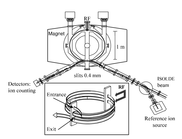
Figure 1: Layout of the Mistral spectrometer (overhead view). The ion beams (coming from the right) are injected either from the Isolde beamline (at 60 keV) or from a reference ion source (variable energy). Inset shows a view of the trajectory envelope with the 0.4 mm entrance slit followed by the first modulator after one-half turn, an opening to accommodate the modulated-ion trajectories after one-turn, the second modulator after three-half turns, and the exit slit.

Figure 2: Accumulated transmission peak for ³³Mg. Due to the weak production rate, a modest mass resolving power of only about 20 000 was used to favor transmission. For more abundant species a resolving power of 100 000 can be obtained.

Figure 3: The $\chi$ values for each of the 23 mass measurements performed during the Rilis experiment in chronological order (a) before adding any ‘static’ instrumental error ($\overline{\chi}=1.4$); (b) after adding a ‘static’ instrumental error of $4\times 10^{-7}$ ($\overline{\chi}=1.0$); (c) after removing measurements 15 and 21 and reducing the ‘static’ instrumental error to $3\times 10^{-7}$ ($\overline{\chi}=1.0$).

Figure 4: Calibration slopes $a=\frac{\Delta_{x}^{meas}}{\frac{\Delta V}{\overline{V}}}$ obtained for ¹⁴N¹⁴N $-^{15}$N¹⁴N (full circles) or ¹⁴N¹⁴N $-^{23}$Na (empty cirles) for various accelerating voltages $\overline{V}$.

Figure 5: Calibration function for the Rilis experiment for all calibrant masses. Top: plotted is the relative mass differences $\Delta^{meas}_{x}$, for the calibrant masses, versus the relative voltage difference $\Delta V/\overline{V}$. The continuous line represents the fit for the linear calibration law (Eq. (9)). Bottom: residual after subtraction of the calibration law.

Figure 6: Comparison of the Rilis measurements with the previously adopted mass values from Ame’95 [13]. The error is a quadratic combination of all sources of errors. The Ame’95 precision is represented by the two symmetric continuous lines. The Plasma results for ^29,32Mg and those of the Thermo experiment for the ²⁶Na are also reported here for comparison.

Figure 7: Dispersion of the measurements corresponding to the same jump amplitude, as compared to the fitted calibration law after addition of $\sigma_{dyn}=7\times 10^{-7}$. A time dependance of $0.5\times 10^{-9}$/min has been subtracted before averaging. The shadowed areas correspond to the 1$\sigma$ limit of the averaged values of each group.

Figure 8: Calibration function for the Plasma experiment for all calibrants taken together. Plotted are the weighted mean values of the relative mass differences $\Delta^{meas}_{x}$ corresponding to the same jump amplitude versus the relative voltage differences $\Delta V/\overline{V}$. The $A$ values are indicated for each input data (the references appear at $\frac{\Delta V}{\overline{V}}=0$). The continuous lines represent the fit for the linear calibration law (Eqs. (14) and (15)). Top: after subtraction of the offsets. Bottom: after subtraction of the full calibration law. The full circles are for the Na reference, and the triangles for the K reference.

Table 1: Calibration data from the Rilis experiment expressed as relative mass differences. The second part gives the averaged results. Column 2 gives the measured value $\Delta^{meas}_{x}$ and column 3, the value corrected for calibration, $\Delta^{corr}_{x}$. The errors between square brackets include only the statistical and the ‘static’ ($3\times 10^{-7}$) errors, while the ones between parentheses include also the ‘dynamic’ error ($4\times 10^{-7}$).

	Nuclide	$\Delta^{meas}_{x}\times 10^{7}$	$\Delta^{corr}_{x}\times 10^{7}$	Nuclide	$\Delta^{meas}_{x}\times 10^{7}$	$\Delta^{corr}_{x}\times 10^{7}$
Individual calibrant masses
	26Mg	$-28.2[1.2](4.2)$	$4.0(4.2)$	24Mg	$-71.3[0.7](4.1)$	$-3.6(4.1)$
	24Mg	$-70.3[1.0](4.1)$	$-2.6(4.1)$	23Na	$-80.3[0.9](4.1)$	$6.1(4.1)$
	25Mg	$-53.8[0.9](4.1)$	$-4.3(4.1)$	24Mg	$-66.9[0.7](4.1)$	$0.8(4.1)$
	23Na	$-86.0[0.6](4.0)$	$0.4(4.0)$	23Na	$-89.3[0.7](4.1)$	$-2.9(4.1)$
	26Mg	$-25.7[0.8](4.1)$	$6.5(4.1)$	26Mg	$-35.6[0.8](4.1)$	$-3.4(4.1)$
	25Mg	$-48.6[0.8](4.1)$	$0.9(4.1)$	28Mg	$-1.1[1.6](4.3)$	$-1.9(4.3)$
Averaged masses
	23Na		$1.2(2.4)$
	24Mg		$-1.8(2.4)$
	25Mg		$-1.7(2.9)$
	26Mg		$2.3(2.4)$
	28Mg		$-1.9(4.3)$

Table 2: Mistral measured masses for the Rilis experiment. In column 2, 3 and 4 are respectively the measured, corrected relative and absolute mass differences. Column 5 and 6 give the deduced mass excess (ME) in $\mu$u and in keV. Column 7 gives the mass excess from the Ame’95 mass table [13]. In the ‘individual measurements’ part, the errors, between square brackets, include only the statistical and the ‘static’ ($3\times 10^{-7}$) errors, while the ones between parentheses include also the ‘dynamic’ error ($4\times 10^{-7}$). In the ‘averaged masses’ part, the errors between parentheses include the ‘calibration’ error (Eq. (13)) added after averaging.

Nuclide	$\Delta^{meas}_{x}\times 10^{7}$	$\Delta^{corr}_{x}\times 10^{7}$	$\delta m_{x}$ ($\mu$u)	ME($\mu$u)	ME(keV)	AME’95(keV)
Individual measurements
30Mg	$26.3[0.7](4.1)$	$-5.4(4.1)$
31Mg	$48.4[1.1](4.2)$	$2.1(4.2)$
32Mg	$20.3[0.3](4.0)$	$-40.2(4.0)$
33Mg	$-9.3[0.9](4.1)$	$-83.5(4.1)$
26Na	$-15.8[0.6](4.0)$	$16.2(4.0)$
30Mg	$27.5[1.1](4.2)$	$-4.2(4.2)$
31Mg	$62.9[2.0](4.5)$	$16.5(4.5)$
30Mg	$30.7[1.4](4.3)$	$-1.0(4.3)$
29Mg	$36.2[1.3](4.2)$	$19.6(4.2)$
Averaged masses
26Na		$16.2(4.3)$	$42(11)$	$-7368(11)$	$-6863(11)$	$-6902(14)$
29Mg		$19.6(5.5)$	$57(16)$	$-11388(16)$	$-10608(15)$	$-10661(29)$
30Mg		$-3.6(4.8)$	$-11(14)$	$-9546(14)$	$-8892(13)$	$-8880(70)$
31Mg		$8.8(5.7)$	$27(18)$	$-3425(18)$	$-3190(16)$	$-3220(80)$
32Mg		$-40.2(6.8)$	$-129(22)$	$-983(22)$	$-915(20)$	$-800(100)$
33Mg		$-83.5(7.3)$	$-276(24)$	$5311(24)$	$4947(22)$	$5200(150)$

Table 3: Calibration data from the Plasma experiment in chronological order, expressed as relative mass differences. The errors, between square brackets, include only the statistical and the ‘static’ ($5\times 10^{-7}$) errors, while the ones between parentheses include also the ‘dynamic’ error ($7\times 10^{-7}$).

Nuclide-Ref.	time (min)	$\Delta^{meas}_{x}\times 10^{7}$	Nuclide-Ref.	time (min)	$\Delta^{meas}_{x}\times 10^{7}$
Individual calibrant masses
23Na-23Na	837	$15.7[0.5](7.0)$	26Mg-23Na	3941	$-42.3[0.9](7.1)$
23Ne-23Na	1166	$17.6[2.9](7.6)$	26Mg-23Na	4233	$-29.2[1.2](7.1)$
23Na-23Na	1216	$17.7[2.4](7.4)$	23Na-23Na	4430	$49.9[0.8](7.0)$
23Ne-23Na	1265	$4.5[1.5](7.2)$	14C15O-23Na	4896	$-95.9[4.2](8.1)$
23Na-23Na	1307	$18.3[1.9](7.3)$	14N15N-23Na	5045	$-91.5[4.3](8.2)$
25Mg-23Na	1382	$-21.8[1.1](7.1)$	29Si-23Na	5050	$-90.1[13.1](14.8)$
25Mg-23Na	1404	$-26.9[1.0](7.1)$	23Na-23Na	5180	$44.7[1.7](7.2)$
25Na-23Na	1614	$-35.2[2.7](7.5)$	23Na-23Na	5355	$53.4[0.9](7.1)$
25Mg-23Na	1644	$-31.1[2.2](7.3)$	26Mg-23Na	5430	$-36.5[2.0](7.3)$
25Mg-23Na	1890	$-28.9[1.4](7.1)$	26Mg-23Na	5520	$-44.7[1.9](7.3)$
27Mg-23Na	2350	$-57.7[1.6](7.2)$	12C18O-41K	5776	$159.0[6.0](9.2)$
27Mg-23Na	2384	$-46.6[2.5](7.4)$	12C18O-41K	5797	$170.3[5.8](9.1)$
27Al-23Na	2499	$-54.8[1.5](7.2)$	15N15N-41K	5810	$169.1[4.0](8.0)$
27Al-23Na	2548	$-42.7[1.3](7.1)$	30Ni-41K	5978	$153.6[1.8](7.2)$
27Al-23Na	2632	$-39.6[2.0](7.3)$	30Ni-39K	5999	$140.3[2.3](7.4)$
27Mg-23Na	2666	$-46.1[2.3](7.4)$	30Ni-39K	6058	$132.4[4.6](8.4)$
23Na-23Na	2918	$20.4[0.6](7.0)$	39Kr-39K	6387	$12.1[4.9](8.6)$
23Na-23Na	3011	$29.4[1.7](7.2)$	41Kr-41K	6452	$24.5[3.8](8.0)$
27Al-23Na	3039	$-49.9[1.3](7.1)$	39K -41K	6990	$22.0[6.5](11.8)$
27Mg-23Na	3052	$-47.3[2.1](7.3)$	30Ni-41K	7170	$157.8[1.5](7.2)$
27Mg-23Na	3400	$-52.7[1.4](7.1)$	30Ni-39K	7247	$135.8[2.0](7.3)$
23Na-23Na	3826	$40.8[2.7](7.5)$	32S -39K	7280	$91.5[2.3](7.4)$
			39K -41K	7620	$20.0[12.1](15.6)$

Table 4: Calibration results (for averaged masses) from the Plasma experiment expressed as relative mass differences. In column 3, are the measured value $\Delta_{x}{}_{t}^{meas}$ after taking into account the time dependance. The errors, between parentheses, include the statistical, the ‘static’ ($5\times 10^{-7}$), and the ‘dynamic’ ($7\times 10^{-7}$) errors. Column 4 gives the value corrected for calibration, $\Delta^{corr}_{x}$. Its error includes also the ’fitting’ error ($9\times 10^{-7}$).

Isolde mass	Mistral mass	$\Delta_{x}{}_{t}^{meas}\times 10^{7}$	$\Delta^{corr}_{x}\times 10^{7}$
23	23	$14.5(2.2)$	$8.1(9.3)$
25	23	$-36.5(3.2)$	$-2.0(9.6)$
26	23	$-61.9(3.6)$	$-8.2(9.7)$
27	23	$-62.3(2.4)$	$9.9(9.3)$
29	23	$-118.1(5.4)$	$-11.1(10.5)$
30	39	$104.1(4.4)$	$0.4(10.0)$
30	41	$130.2(3.6)$	$2.4(9.7)$
39∗	41	$21.4(7.9)$	$-3.2(12.0)$
$[41]^{**}$	$[41]^{**}$	$-13.4(5.8)$	$11.3(10.7)$
32	39	$55.1(7.4)$	$-17.3(11.6)$
* mass from Mistral
** mean value of 41K+-82Kr++ and 39K+-78Kr++ measurements

Table 5: Mistral measured masses for the Plasma experiment using the new calibration law. In column 2 is the measured mass difference, in column 3 the averaged mass difference after taking into account the time dependance (Eqs. (14) and (15)), in column 4 the corrected relative mass difference (Eq. (12)) and in column 5 the absolute mass difference. In the ‘individual measurements’ part, the error in column 2 includes only the statistical and the ‘static’ errors ($5\times 10^{-7}$), in column 3 the ‘dynamic’ error ($7\times 10^{-7}$) is added, and in column 4 the ‘fitting’ error ($9\times 10^{-7}$) is added. In the ‘averaged masses’ part, the error in columns 4 and 5 includes also the ‘calibration’ error.

Nuclide-Ref.	time(min)	$\Delta^{meas}_{x}\times 10^{7}$	$\Delta_{x}{}_{t}^{meas}\times 10^{7}$	$\Delta^{corr}_{x}\times 10^{7}$	$\delta m_{x}$ ($\mu$u)
Individual measurements
29Mg-23Na	4901	$-73.2(3.2)$	} $-94(5)$	$13(10)$
29Mg-23Na	4943	$-65.4(1.6)$
26Ne-23Na	5530	$-18.9(1.6)$	$-47(7)$	$7(12)$
32Mg-39K	7540	$78.0(10.3)$	$40(12)$	$-32(15)$
32Mg-41K	7700	$98.0(7.8)$	$60(10)$	$-37(14)$
Averaged masses
26Ne			$7(13)$	$18(34)$
29Mg			$13(13)$	$38(38)$
32Mg			$-35(12)$	$-112(38)$

Table 6: Mistral measured masses for the Plasma experiment using the isobaric data. In columns 2 and 3 are the averaged measured relative mass differences for, respectively, the nuclide of interest and the average isobaric reference. Column 4 is the difference between the two preceding columns and is equivalent to $\Delta^{corr}_{x}$. Column 5 is the absolute mass difference. All the errors include the statistical, the ‘static’ ($5\times 10^{-7}$), and the ‘dynamic’ ($6\times 10^{-7}$) errors.

Nuclide-Ref.	$\Delta^{meas}_{x}\times 10^{7}$	$\Delta^{meas}_{r}\times 10^{7}$	$\Delta_{x-r}\times 10^{7}$	$\delta m_{x}$ ($\mu$u)
26Ne-26	$-18.9(6.2)$	$-40.6(4.5)$	$22(8)$	$56(20)$
29Mg-29	$-69.0(4.6)$	$-93.3(4.9)$	$24(7)$	$70(19)$

Table 7: Mistral measured masses for the Plasma experiment. In column 2 is the absolute mass difference. Columns 3 and 4 give the deduced mass excess (ME) in $\mu$u and in keV. The errors take into account all sources of errors. Column 5 gives the mass excess from the Ame’95 mass table [13].

Nuclide-Ref.	$\delta m_{x}$ ($\mu$u)	ME($\mu$u)	ME(keV)	AME’95(keV)
26Ne	$56(20)$	$518(20)$	$482(18)$	$430(50)$
29Mg	$70(19)$	$-11375(19)$	$-10596(18)$	$-10661(29)$
32Mg	$-112(38)$	$-966(38)$	$-900(36)$	$-800(100)$

Table 8: Calibration parameters from the Thermo experiment determined for each of the measurement periods, after addition of the ‘fitting’ error of 4$\times 10^{-7}$. In column 4, the correlation coefficients ($\sigma^{2}_{ab}$) between the fitted parameters $a$ and $b$ are given. The $\chi$ values of the calibration fits are given in column 5. This table supersedes Table II of ref. [5].

Set	Slope			Offset			$\sigma^{2}_{ab}$	$\chi$
	($a\times 10^{7}$)			($b\times 10^{7}$)
#1a	$210.$	$\,($	16.)
#1b	$232.$	$\,($	10.)	$1.7$	$\,($	4.0)	$-33.5$	0.5
#2a	$26.5$	$\,($	9.5)	$-4.6$	$\,($	2.9)	$-14.3$	0.4
#2b	$83.1$	$\,($	5.8)	$-4.5$	$\,($	1.9)	$-6.6$	1.1
#2c	$-17.1$	$\,($	4.6)	$-2.8$	$\,($	1.7)	$-5.1$	0.8
#2d	$-35.0$	$\,($	38.)	$-3.0$	$\,($	3.9)	$107.$	0.2

Table 9: Calibration results from the Thermo experiment expressed as relative mass differences. The second part gives the averaged results. In column 2, the measured value $\Delta^{meas}_{x}$ is shown. The error, between parentheses, is the statistical error. Column 3 gives the value corrected for calibration, $\Delta^{corr}_{x}$. Its error includes the ‘fitting’ error ($4\times 10^{-7}$). This table supersedes Tables I+III+V of ref. [5].

Nuclide-Ref.	$\Delta^{meas}_{x}\times 10^{7}$	$\Delta^{corr}_{x}\times 10^{7}$	Nuclide-Ref.	$\Delta^{meas}_{x}\times 10^{7}$	$\Delta^{corr}_{x}\times 10^{7}$
Individual calibrant masses
set#1a			set#2c
$\quad{}^{27}$Al-39K	$78.0(0.5)$	$0.(4.0)$	$\quad{}^{23}$Na-23Na	$-1.5(1.3)$	$1.3(4.2)$
set#1b			$\quad{}^{23}$Na-39K	$-7.1(1.4)$	$4.5(4.2)$
$\quad{}^{25}$Na-39K	$103.5(0.6)$	$0.4(4.0)$	$\quad{}^{25}$Na-23Na	$-2.8(1.5)$	$-1.4(4.3)$
$\quad{}^{24}$Na-39K	$113.7(0.6)$	$1.6(4.0)$	$\quad{}^{25}$Na-39K	$-8.3(1.9)$	$2.0(4.4)$
$\quad{}^{23}$Na-23Na	$1.5(0.5)$	$-0.2(4.0)$	$\quad{}^{23}$Na-23Na	$-2.6(1.5)$	$0.2(4.3)$
$\quad{}^{23}$Na-39K	$119.5(0.7)$	$-1.8(4.1)$	$\quad{}^{23}$Na-39K	$-8.0(1.4)$	$3.6(4.2)$
set#2a			$\quad{}^{24}$Na-23Na	$-4.1(1.3)$	$-2.0(4.2)$
$\quad{}^{23}$Na-23Na	$-3.9(2.4)$	$0.7(4.7)$	$\quad{}^{24}$Na-39K	$-15.2(1.4)$	$-4.3(4.2)$
$\quad{}^{25}$Na-23Na	$-7.1(1.3)$	$-0.3(4.2)$	$\quad{}^{27}$Al-23Na	$2.1(1.0)$	$2.2(4.1)$
$\quad{}^{25}$Na-39K	$4.9(3.0)$	$-2.1(5.0)$	$\quad{}^{27}$Al-39K	$-10.9(1.1)$	$-1.9(4.2)$
set#2b			set#2d
$\quad{}^{23}$Na-23Na	$-5.6(1.4)$	$-1.1(4.2)$	$\quad{}^{23}$Na-23Na	$-3.2(0.6)$	$-0.1(4.0)$
$\quad{}^{23}$Na-39K	$38.1(2.1)$	$-0.3(4.5)$	$\quad{}^{26}$Na-23Na	$18.9(0.8)$	$17.7(4.4)$
$\quad{}^{25}$Na-23Na	$-13.3(1.9)$	$-1.9(4.4)$	$\quad{}^{28}$Na-23Na	$20.4(6.0)$	$16.7(8.2)$
$\quad{}^{25}$Na-39K	$36.8(1.0)$	$4.9(4.1)$
$\quad{}^{27}$Al-23Na	$-14.5(1.8)$	$3.3(4.4)$
$\quad{}^{27}$Al-39K	$17.8(1.1)$	$-7.9(4.2)$
$\quad{}^{23}$Na-23Na	$-3.6(1.6)$	$0.9(4.3)$
Averaged masses
$\quad{}^{23}$Na		$0.7(1.3)$
$\quad{}^{24}$Na		$-1.5(2.4)$
$\quad{}^{25}$Na		$0.4(1.6)$
$\quad{}^{27}$Al		$-1.1(2.1)$

Table 10: Mistral results from the Thermo experiment expressed as relative mass differences. In columns 2 and 3 are, respectively, the measured and corrected relative mass difference. The second part, ‘** Averaged masses for set#2c’, gives the averaged results only for measurements which have been repeated inside a set. The errors, in column 2, are the statistical errors. In column 3, the errors, between square brackets, include also the ‘fitting’ error ($4\times 10^{-7}$), while for the ones between parentheses the ‘calibration’ error is added. This table supersedes Tables I+III of ref. [5].

Nuclide-Ref.	$\Delta^{meas}_{x}\times 10^{7}$	$\Delta^{corr}_{x}\times 10^{7}$	Nuclide-Ref.	$\Delta^{meas}_{x}\times 10^{7}$	$\Delta^{corr}_{x}\times 10^{7}$
Individual masses
set#1a			set#2c
$\quad{}^{27}$Na-39K	$103.0(1.2)$	$25.0[4.2](7.1)$	$\quad{}^{28}$Na-23Na	$25.2(6.0)$	$24.6[7.2](7.5)$
$\quad{}^{28}$Na-39K	$91.2(4.5)$	$20.6[6.0](8.0)$	$\quad{}^{28}$Na-39K	$1.9(8.1)$	$10.3[9.0](9.2)$
set#1b			$\quad{}^{29}$Na-23Na	$26.1(6.2)$	$25.0[7.4](7.7)$
$\quad{}^{29}$Na-39K	$95.5(7.0)$	$25.6[8.1](8.9)$	$\quad{}^{29}$Na-39K	$-0.1(6.3)$	$7.7[7.5](7.7)$
$\quad{}^{26}$Na-39K	$100.0(0.5)$	$5.6[4.0](5.8)$	$\quad{}^{26}$Na-23Na	$20.1(1.0)$	$20.8[4.1]**$
$\quad{}^{30}$Na-39K	$-13.2(9.7)$	$-75.4[10.5](11.1)$	$\quad{}^{26}$Na-39K	$12.1(1.0)$	$21.7[4.1]**$
set#2a			$\quad{}^{26}$Na-23Na	$21.3(1.5)$	$22.0[4.3]**$
$\quad{}^{26}$Na-23Na	$11.8(1.3)$	$19.6[4.2](5.4)$	$\quad{}^{26}$Na-39K	$10.3(1.5)$	$19.9[4.3]**$
$\quad{}^{26}$Na-39K	$28.0(2.0)$	$22.0[4.5](6.1)$	$\quad{}^{27}$Na-23Na	$23.1(2.2)$	$23.2[4.6](5.0)$
set#2b			$\quad{}^{27}$Na-39K	$17.2(1.4)$	$26.2[4.2](4.7)$
$\quad{}^{26}$Na-23Na	$-7.7(1.9)$	$6.9[4.4](5.0)$	set#2d
$\quad{}^{26}$Na-39K	$43.7(2.6)$	$15.0[4.8](5.4)$	$\quad{}^{30}$Na-23Na	$-77.6(9.0)$	$-83.7[9.9](13.7)$
$\quad{}^{28}$Na-39K	$33.0(9.1)$	$10.2[9.9](10.2)$
** Averaged masses for set#2c
$\quad{}^{26}$Na-23Na		$21.4[3.0](3.5)$
$\quad{}^{26}$Na-39K		$20.9[3.0](3.6)$

Table 11: Mistral measured masses for the Thermo experiment. In column 2 and 3 are respectively the corrected relative and absolute mass differences. Columns 4 and 5 give the deduced mass excess (ME) in $\mu$u and in keV. Column 6 gives the mass excess from the Ame’95 mass table [13]. The errors in columns 2-5 take into account all sources of errors. This table supersedes Tables VI of ref. [5].

Nuclide	$\Delta^{corr}_{x}\times 10^{7}$	$\delta m_{x}$ ($\mu$u)	ME($\mu$u)	ME(keV)	AME’95(keV)
26Na	$17.3(1.6)$	$45(4)$	$-7365(4)$	$-6860(4)$	$-6902(14)$
27Na	$25.2(1.5)$	$68(4)$	$-5922(4)$	$-5516(4)$	$-5580(40)$
28Na	$17.6(3.8)$	$49(11)$	$-1061(11)$	$-988(10)$	$-1030(80)$
29Na	$18.9(4.6)$	$55(13)$	$2866(13)$	$2669(12)$	$2620(90)$
30Na	$-78.5(8.4)$	$-236(25)$	$8990(25)$	$8375(23)$	$8590(90)$

Table 12: Summary of the new reevaluated Mistral results.

Nuclide	ME($\mu$u)	ME(keV)	Experiment
26Na	$-7368(11)$	$-6863(11)$	Rilis
29Mg	$-11388(16)$	$-10608(15)$
30Mg	$-9546(14)$	$-8892(13)$
31Mg	$-3425(18)$	$-3190(16)$
32Mg	$-983(22)$	$-915(20)$
33Mg	$5311(24)$	$4947(22)$
26Ne	$518(20)$	$482(18)$	Plasma
29Mg	$-11375(19)$	$-10596(18)$
32Mg	$-966(38)$	$-900(36)$
26Na	$-7365(4)$	$-6860(4)$	Thermo
27Na	$-5922(4)$	$-5516(4)$
28Na	$-1061(11)$	$-988(10)$
29Na	$2866(13)$	$2669(12)$
30Na	$8990(25)$	$8375(23)$

Table 13: New adjustment of the data related to ²⁶Na taking into account our data from Table 12. Column 2 is the measured value in $\mu$u for mass-spectrometry and in keV for reactions and decays. Column 3 is the output of a least-squares fit of all available experimental data as in Ame’2003 (Ref. [14], p. 184). Column 4 gives the difference between the measured and adjusted values relative to the uncertainty of the measured value.

Measurement	Measured value	Adjusted value	$v_{i}$	Reference
26Na	$-7365(4)$	$-7365(4)$	$-0.1$	Thermo
26Na	$-7368(11)$	$-7365(4)$	$0.2$	Rilis
26Na($\beta^{-}$)26Mg	$9210(200)$	$9354(4)$	$0.7$	[18]
26Mg(7Li,7Be)26Na*	$-10182(40)$	$-10216(4)$	$-0.8$	[19]
26Mg($t$,3He)26Na	$-9292(20)$	$-9335(4)$	$-2.2$	[20]
25Na$-.721\times^{26}$Na$-.284\times^{22}$Na	$-2881(33)$	$-2940(4)$	$-1.8$	[21]
25Na$-.721\times^{26}$Na$-.284\times^{22}$Na	$-2921(22)$	$-2940(4)$	$-0.8$	[21]
26Na$-.770\times^{27}$Na$-.236\times^{22}$Na	$-1437(86)$	$-1389(5)$	$0.6$	[21]
26Na$-.481\times^{27}$Na$-.520\times^{25}$Na	$676(66)$	$658(6)$	$-0.2$	[21]
26Na$-.481\times^{27}$Na$-.520\times^{25}$Na	$734(86)$	$658(6)$	$-0.6$	[21]
26Na$-.619\times^{28}$Na$-.394\times^{22}$Na	$-4229(613)$	$-4208(7)$	$0.0$	[21]
26Na$-.619\times^{28}$Na$-.394\times^{22}$Na	$-4205(128)$	$-4208(7)$	$0.0$	[21]
26Na$-.619\times^{28}$Na$-.394\times^{22}$Na	$-4203(87)$	$-4208(7)$	$-0.1$	[21]
26Na$-.512\times^{29}$Na$-.506\times^{22}$Na	$-5763(91)$	$-5606(7)$	$1.2$	[21]
26Na$-.512\times^{29}$Na$-.506\times^{22}$Na	$-6379(293)$	$-5606(7)$	$1.8$	[21]
26Na$-.512\times^{29}$Na$-.506\times^{22}$Na	$-5252(277)$	$-5606(7)$	$-0.5$	[21]
26Na$-.512\times^{29}$Na$-.506\times^{22}$Na	$-5576(66)$	$-5606(7)$	$-0.5$	[21]
26Na$-.433\times^{30}$Na$-.591\times^{22}$Na	$-7454(287)$	$-7425(24)$	$0.1$	[21]
26Na$-.433\times^{30}$Na$-.591\times^{22}$Na	$-8060(641)$	$-7425(24)$	$0.7$	[21]
26Na$-.433\times^{30}$Na$-.591\times^{22}$Na	$-7045(225)$	$-7425(24)$	$-0.7$	[21]
26Na$-.433\times^{30}$Na$-.591\times^{22}$Na	$-7515(117)$	$-7425(24)$	$0.8$	[21]
* The original result, Q$=-10222(30)$ keV, has been corrected (see text).

References

- [1] D. Lunney, J.M. Pearson and C. Thibault, Rev. Mod. Phys. 75 (2003) 1021.
- [2] D. Lunney, C. Gaulard, G. Audi, M. de Saint Simon, C. Thibault and N. Vieira, Eur. Phys. J. A (2004) submitted, http://hal.ccsd.cnrs.fr/ccsd-00003131.
- [3] C. Monsanglant, Doctoral Thesis #6283, Université Paris-Sud, Orsay, 2000; http://www.nndc.gov/amdc/experimental/th-monsangl.pdf
- [4] D. Lunney, G. Audi, H. Doubre, S. Henry, C. Monsanglant, M. de Saint Simon, C. Thibault, C. Toader, C. Borcea, G. Bollen and the Isolde Collaboration, Hyperfine Interact. 132 (2001) 299.
- [5] D. Lunney, G. Audi, H. Doubre, S. Henry, C. Monsanglant, M. de Saint Simon, C. Thibault, C. Toader, C. Borcea, G. Bollen and the Isolde Collaboration, Phys. Rev. C 64 (2001) 054311.
- [6] M. de Saint Simon, C. Thibault, G. Audi, A. Coc, H. Doubre, M. Jacotin, J.F. Képinski, R. Le Gac, G. Le Scornet, D. Lunney and F. Touchard, Phys. Scripta T59 (1995) 406.
- [7] M.D. Lunney, G. Audi, C. Borcea, M. Dedieu, H. Doubre, M. Duma, M. Jacotin, J.F. Képinski, G. Le Scornet, M. de Saint Simon and C. Thibault, Hyperfine Int. 99 (1996) 105.
- [8] A. Coc, R. Le Gac, M. de Saint Simon, C. Thibault and F. Touchard, Nucl. Instrum. Methods A 271 (1988) 512.
- [9] N. Vieira, Doctoral Thesis, Université Paris VI, Paris, 2002; http://www.nndc.gov/amdc/experimental/th-vieira.pdf
- [10] C. Bachelet, Doctoral Thesis, Université Paris XI, Orsay, 2004; http://www.nndc.gov/amdc/experimental/th-bachelet.pdf
- [11] E. Kugler, Hyperfine Interact. 129 (2000) 23.
- [12] http://www.nndc.gov/amdc/experimental/masstables/Ame1995/mass_rmd.mas95
- [13] G. Audi and A.H. Wapstra, Nucl. Phys. A 595 (1995) 409.
- [14] G. Audi, A.H. Wapstra and C. Thibault, Nucl. Phys. A729 (2003) 337; A.H. Wapstra, G. Audi and C. Thibault, Nucl. Phys. A729 (2003) 129.
- [15] A. Coc, R. Fergeau, R. Grabit, M. Jacotin, J.F. Képinski, R. Le Gac, G. Le Scornet, G. Petrucci, M. de Saint Simon, G. Stefanini, C. Thibault and F. Touchard, Nucl. Instrum. Methods A 305 (1991) 143.
- [16] H. Nann, K.K. Seth, S.G. Iversen, M.O. Kaletka, D.B. Barlow and D. Smith, Phys. Lett. B 96 (1980) 261.
- [17] N.A. Orr et al, Phys. Lett. B 258 (1991) 29.
- [18] D.E. Alburger, D.R. Goosman, C.N. Davids, Phys. Rev. C 8 (1973) 1011.
- [19] G.C. Ball, W.G. Davies, J.S. Forster, J.C. Hardy, Phys. Rev. Lett. 28 (1972) 1069.
- [20] E.R. Flynn, J.D. Garrett, Phys. Rev. C 9 (1974) 210.
- [21] C. Thibault, R. Klapisch, C. Rigaud,. A.M. Poskanzer, R. Prieels, L. Lessard, W. Reisdorf, Phys. Rev. C 12 (1975) 644.
- [22] F. Sarazin et al, Phys. Rev. Lett. 84 (2000) 5062.