Jet Study in Ultra-Relativistic Heavy-Ion Collisions with the ALICE Detectors at the LHC

In ultra-relativistic heavy-ion collisions at $\sqrt{s_{NN}}$ = 5.5 TeV at the ALICE experiment at the LHC, interactions between the high-$p_{T}$ partons and the hot, dense medium produced in the collisions, are expected to lead to jet energy loss (jet-quenching) resulting in changes in the jet fragmentation functions as compared to the unquenched case. In order to reconstruct jet fragmentation functions, accurate information on the jet energy, direction and momentum distribution of the jet particles is needed. This thesis presents first results on jet reconstruction in simulated Pb+Pb collisions using the ALICE detectors and a UA1-based cone jet finding algorithm which has been modified and optimised to reconstruct high-$p_{T}$ jets on an event-by-event basis. Optimisation of the algorithm parameters and methods used to suppress the large background energy contribution while maximising the algorithm efficiency, are discussed and the resulting jet energy and direction resolutions are presented. Accurate jet reconstruction will allow measurement of the jet fragmentation functions and consequently the degree of quenching and therefore provide insight on the properties of the hot and dense medium (for example the initial gluon density) created in the collisions.

Publications and presentations on this work include:

1. S-L Blyth, Jet study in ultra-relativistic heavy-ion collisions with the ALICE detector at the LHC. Talk presented at Quark Matter 2004 Conference, Oakland, California, USA, January 2004

2. S-L Blyth, Jet study in ultra-relativistic heavy-ion collisions with the ALICE detector at the LHC. Paper to be published in Journal of Physics G: Nuclear and Particle Physics, QM2004 proceedings

3. S-L Blyth and M. J. Horner, Jet Study in Ultra-relativistic Heavy-ion Collisions at the LHC. Poster presented at the Gordon Conference on Nuclear Chemistry, New Hampshire, USA, June 2004

Acknowledgements

There are many people I’d like to thank that helped me in one way or another (or in many ways!) in producing this thesis:

Thank you Prof. Cleymans and Grazyna for allowing me to spend time at Lawrence Berkeley National Laboratory and work on this very interesting topic. It has been a very exciting time and a great opportunity.

Thank you Grazyna, Jenn, Spencer and Mark for all your patience, input and help. I greatly appreciate it. I’d also like to thank Heather, Marco, Andreas, Tom, Alexei and the rest of the ALICE and ALICE-USA collaborations for your help.

Thank you Mark for teaching me ROOT, for all your encouragement and for generally putting up with me!

Thank you Mom and Dad for making me believe I could do it.

ContentstocList of FigureslofList of Tableslot

Chapter 1 Introduction

1.1 Heavy-ion Collisions and the QGP

The ultimate goal of ultra-relativistic heavy-ion collision experiments is to create and study the quark-gluon plasma (QGP), a phase of matter in which quarks and gluons move freely in thermal and chemical equilibrium [2]. The QGP is predicted by the theory of quantum chromodynamics (QCD) [3]; the theory of the strong colour force which is responsible for binding the constituent quarks and gluons (collectively called partons) inside nucleons i.e. protons and neutrons [4].

In nature, quarks are never found alone. Instead, they are always found bound together in threes, inside baryons, or twos, as quark-antiquark pairs inside mesons. This feature of QCD, that the effective coupling constant $\alpha_{s}(Q^{2})$ between quarks increases at low temperature and momentum transfer $Q$, or large distances, is called confinement. However in QCD, at high temperature and momentum transfer $Q$, or short distances ($\sim$1 fm), $\alpha_{s}(Q^{2})$ decreases logarithmically and the quarks become asymptotically free or deconfined [5, 6].

1.1.1 The QCD Phase Diagram

According to the standard model, the evolution of the early universe included a QGP phase at a very early stage (a few microseconds after the Big Bang) before it cooled down and the quarks and gluons hadronised into ordinary nuclear matter.

A sketch of the QCD phase diagram [7] of temperature versus baryon chemical potential ($T$ vs. $\mu_{B}$) is shown in Fig. 1.1. As temperature increases, the coupling between quarks becomes weak leading to deconfinement of the quarks and chiral symmetry restoration (the quarks appear as nearly massless particles compared to having masses of the order of more than 100 MeV when they are confined inside hadrons). This state of freely moving quarks and gluons, close to or at equilibrium, QGP, is predicted by QCD and indicated in Fig. 1.1 above the curved line.

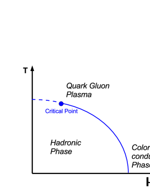
Fig. 1.1: Sketch of QCD phase diagram indicating the critical point for the case of two light quarks and 1 heavy quark. The solid line indicates a first order phase transition and the dashed line indicates a crossover transition. Based on [7].

In QCD, analytical calculations can be performed using perturbative methods (pQCD) above a scale set by $\lambda_{QCD}\approx$ 2 GeV. Below this limit, due to divergences, the equations cannot be solved analytically. Another approach to solving the equations of QCD, is to use non-perturbative lattice gauge theory techniques. This method attempts to discretise, on a lattice, the continuous integral describing the QCD partition function and is complicated due to the increase in calculation complexity as a function of decreasing the step-size of the lattice and requires large computing resources.

Lattice gauge theory calculations predict that at zero chemical potential ($\mu_{B}=0$) the critical temperature at which the phase transition from a hadron gas to a QGP occurs is $T_{c}=160-170$ MeV (e.g. $T_{c}=172\pm 3.5$ MeV in [8]) which relates to an energy density of 1-2 GeV/$\rm{fm^{3}}$ . The order of the phase transition (i.e. first order, second order or a crossover) at $\mu_{B}=0$ is model dependent. For a first order phase transition, the Gibbs energies of the two phases are equal at the transition temperature but the first derivatives with respect to pressure and temperature are discontinuous at the point of transition. A second order phase transition is one where the entropy of the two phases on each side of the phase boundary is the same. A cross-over means that there is no discontinuity in between the phases of the matter involved in the transition, i.e the thermodynamic quantities change smoothly. For cases with 2 light quarks and 1 heavy quark such that $m_{s}\gg m_{u,d}\neq 0$, a smooth crossover is predicted[8, 10], see Fig. 1.1. At large $\mu_{B}$, models predict that the phase transition is of the first order. Thus the first order phase transition line may end at some critical point ($\mu_{E},T_{E}$) in the phase diagram where for $\mu<\mu_{E}$ the transition is a crossover. The position of this critical point is not yet established although some attempts have been made to calculate its position using lattice calculations[8].

At low temperature and very high baryon density (indicated in Fig. 1.1 by high baryon chemical potential, $\mu_{B}$), chiral symmetry is also predicted to be restored. A state of deconfined quarks and gluons may exist within neutron stars in the form of a color superconducting state [10] where quarks may form Cooper pairs bound together by gluons.

1.1.2 Heavy-ion Collisions

QCD predicts that the energy density $\epsilon$ at mid-rapidity grows logarithmically with the centre-of-mass energy of a collision and with $A^{2/3}$, where $A$ is the nuclear mass of the particles involved in the collision [11]. Thus heavy-ion collisions at relativistic energies are an ideal tool to create, in the laboratory, the high energy densities to test the predictions of QCD and the expected formation of the hypothetical state of deconfined matter, the QGP [12].

In the centre-of-mass frame of a relativistic heavy-ion collision, the colliding nuclei appear as two Lorentz-contracted discs as they fly towards each other. When the nuclei collide, they deposit a large amount of energy (dependent on the amount of energy carried by each nucleus) into a very small volume. If the energy density created in the collision is high enough to create a fireball of deconfined quarks and gluons and the system lives long enough that the quarks and gluons have time to interact and thermalise, then a QGP will be created. As the fireball continues expanding rapidly, it cools down and hadronisation occurs. The hadronisation mechanisms involved at different momentum ranges are described phenomenologically.

As the system continues expanding, inelastic and elastic scatterings occur between the particles. Chemical freeze-out occurs when the inelastic scatterings between the hadrons stop. Thermal freeze-out occurs once the elastic scatterings between particles stop i.e. the system has expanded to the point where the particles can no longer interact with each other. Experiments measure the properties of the hadrons after thermal freeze-out.

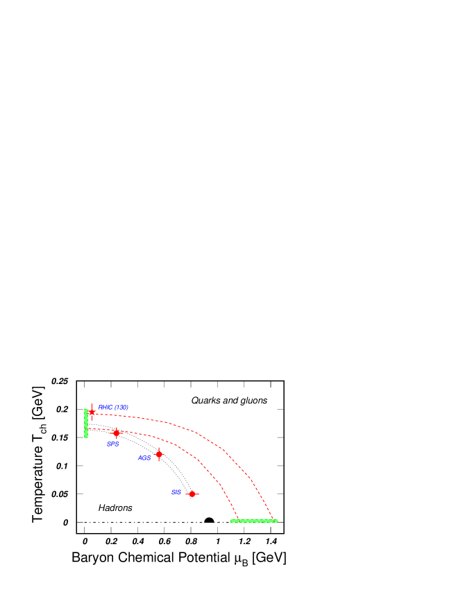
Fig. 1.2: QCD phase plot from [13]. The dashed lines indicate the boundary between interactions involving hadronic and partonic degrees of freedom. The black half circle represents the ground state of nuclei.

Heavy-ion experiments have covered a broad range of energies and masses of colliding nuclei, providing a large amount of data to constrain theoretical calculations. Using a small number of particle ratios, (enough to constrain the model parameters), the temperature $T$, and the baryon density $\mu_{B}$ at thermal freeze-out have been calculated using statistical thermal models at various energies, see Fig. 1.2 from [13]. The values of $T$ and $\mu_{B}$ obtained from the thermal model fits are found to describe well the majority of other particle ratios observed experimentally [13, 14, 15]. In Fig. 1.2, the $T$ and $\mu_{B}$ of the created systems from different heavy-ion experiments, calculated using the thermal model, are plotted along the dotted lines. The collision energy of the experiments increases towards the $T$-axis. Thus the experiments at RHIC measure systems which have calculated values of $T$ and $\mu_{B}$ which are at the boundary of the phase transition at very low baryon density. The Large Hadron Collider (LHC) experiments, scheduled to go online in 2007, will measure systems produced with a collision energy $\sim 30$ times that of RHIC and which are expected to have energy densities about 20 times greater and thus initial temperatures of $T_{LHC}\approx 2.1T_{RHIC}$ [16].

1.2 Probes of the Hot, Dense, Partonic Medium/QGP

Since a hypothetical QGP, if created in a heavy-ion collision, will have an extremely short life-time ($\sim 5-10$ fm/$c$) before hadronisation occurs [11], its presence and characteristics can only be determined using indirect observables. A variety of signatures has been proposed although experimental measurements are complicated due to the time/space evolution of the system and final state hadronic interactions.

The proposed experimental signatures may provide information on different characteristics of the system produced in the collision. For example, proposed signatures of deconfinement include suppression of quarkonium production [17] and enhancement of multi-strange particle production [18]. Chiral symmetry restoration is expected to be observed through measuring modifications of vector meson masses [19]. Hard probes [20] such as high-$p_{T}$ jets, dileptons or direct photons [21], heavy quarkonia or $W^{\pm}$ or $Z^{0}$ may also be used to study the thermalisation of the partons and early stage evolution of the QGP. Hard probes are created in high-$Q^{2}$ interactions and at early times where $\tau_{hard}\sim 1/Q\leq 0.01$ fm/$c$. The bulk of the secondary matter is formed later at around $\tau\sim 1/T_{0}\sim 0.2$ fm/$c$. Thus the hard probe becomes embedded in the secondary matter and as it traverses the hot, dense medium it undergoes softer secondary interactions. Properties of the hard probe may therefore be modified due to medium effects and provide information on properties of the medium, most notably, the initial gluon density. Properties of the system such as energy density $\epsilon$, temperature $T$, and pressure $P$, may be measured using the resulting hadron rapidity and transverse energy distributions as well as the flow distributions [11].

1.2.1 High-$p_{T}$ Jets and Energy Loss in the Medium

This thesis will focus on a specific hard-probe, namely high-$p_{T}$ jets. Jets, which result from hard parton-parton scatterings, have been observed in $e^{+}$+$e^{-}$, p+p and p+$\overline{\rm{p}}$ experiments. A working definition of a jet is a localised (in space) group of hadrons which originate from the fragmentation of an initial hard scattered parton, see Fig. 1.3 [22]. The jet particles are contained within a cone of radius $R=\sqrt{(\Delta\eta)^{2}+(\Delta\phi)^{2}}=1$. The total energy and direction of the jet is expected to be closely related to that of the parent parton.

It has been predicted that a high-$p_{T}$ parton traversing hot nuclear matter, for example a QGP, will experience collisional energy loss (via scattering) and radiative energy loss (via induced gluon bremsstrahlung) [20, 23, 24]. Radiative energy loss is expected to dominate over collisional energy loss. The amount of energy loss, $\Delta E$, is predicted to be proportional to the gluon/energy density of the medium and a function of the path length of the parton through the medium. Thus jets, which have lost energy while traversing the medium, can be used as tools to probe the medium and provide information on its properties and structure at an early stage [20].

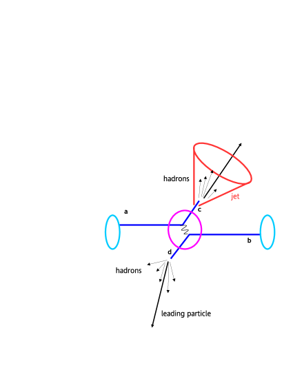
Fig. 1.3: The formation of a di-jet event from the hard scattering of partons (a and b) from nucleons within the incoming nuclei. The hard partons (c and d) traverse the medium formed in the collision (purple circle) before fragmenting into jets of hadrons. From [22].

The pQCD-based calculations in [25] predict that the angular energy distribution for jets which have undergone energy-loss in a dense QCD medium is very similar to the energy distribution of jets which fragment in vacuum, see Fig. 1.4 from [25].

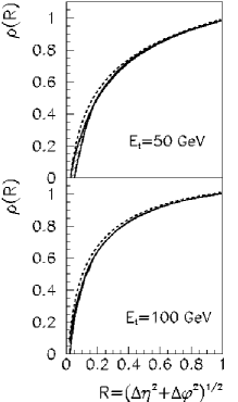
Fig. 1.4: Fraction of total jet $E_{T}$, $\rho(R)$, for quark-led jets fragmenting in vacuum (dashed line) and fragmenting in a dense QCD medium (solid line) based on pQCD calculations from [25] . The upper panel represents the case for a 50GeV jet and the lower panel the case for a 100GeV jet. From [25].

The gluons are radiated at angles close to the jet axis [25] and therefore remain iside the jet cone, see Fig. 1.5. Therefore, measuring the total energy within a cone of radius $R$ (where $R=\sqrt{{(\Delta\eta)}^{2}+{(\Delta\phi)}^{2}}$ ) around the jet axis will not provide information on jet energy loss since the total energy inside the cone will include both the final jet energy plus the radiated energy.

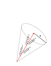
Fig. 1.5: During radiative energy loss, gluons (coiled lines) are radiated at angles close to the jet-axis (arrow) resulting in the total energy inside the cone remaining unchanged [25]. Picture from [22].

However, the momentum distribution of the particles within the jet cone is expected be modified for jets which have lost energy due to medium effects [24]. This in turn causes a modification of the jet fragmentation functions which are defined following [26] as

$$D(z)=\frac{1}{N_{jets}}\frac{dN_{ch}}{dz}$$ (1.1)

where,

$$z=p_{L}/E_{T_{jet}},$$ (1.2)

$p_{L}$ is the momentum component of a particle in the jet in the direction parallel to the jet axis and $E_{T_{jet}}$ is the transverse energy of the jet ($E_{T}=E\sin\theta$). The jet energy loss can be quantified by measuring the jet fragmentation functions and comparing to fragmentation functions measured in p+p collisions or peripheral heavy-ion collisions [24], see Fig. 1.6.

Fig. 1.6 from [24] shows the calculated ratio of the inclusive jet fragmentation functions of jets with energy loss versus jets with no energy loss as a function of the fractional momenta $z$ (where, in this case $z=p_{T}/E_{T_{jet}}$, differing from the definition in equation 1.2) of the jet hadrons. Jet energy loss is manifested by a shift of the fragmentation function towards low $z$, as shown by the increase above unity of low momentum (i.e. low-$z$) particles and the decrease in the number of high-$z$ particles compared to the case with no energy loss i.e there is a shift of particles from high-$p_{T}$ to low-$p_{T}$. Lower energy jets are more affected than higher energy jets as shown in Fig. 1.6.

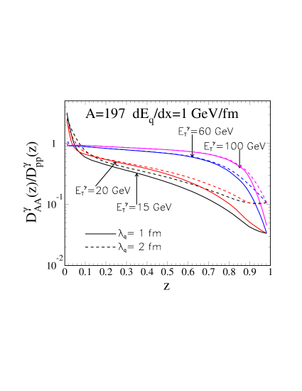
Fig. 1.6: Ratio of the inclusive jet fragmentation functions for $\gamma$-tagged jets with energy loss to the fragmentation function of jets without energy loss in central Au+Au collisions. The solid lines indicate the calculation for the case of inelastic scattering mean free path $\lambda_{q}=$ 1 fm and the dashed line is the case for $\lambda_{q}$ = 2 fm. From [24].

As yet, there is no Monte Carlo event generator which can be used to simulate jet energy loss in a medium in heavy-ion collisions. However, a ‘toy’ model of jet energy loss has been constructed [27]. A jet in a heavy-ion collision is modeled by the superposition of a p+p jet event from PYTHIA [28] on a high-multiplicity A+A event simulated using HIJING [29]. In PYTHIA, jets were modified according to the ‘toy’ model prescription and, for example 20$\%$ energy loss from a 100 GeV jet, was mocked up by superimposing a 20 GeV PYTHIA jet on an 80 GeV PYTHIA jet on top of a HIJING background event. Fig. 1.7 shows the resulting modified fragmentation function from a sample of 100 GeV jets with energy loss modeled in this way compared to the fragmentation function from 100 GeV jets with no energy loss. The fragmentation function for the energy-loss case is shifted to lower $p_{T}$ as expected. The magnitude of the shift may provide information on the medium properties. Thus, in experiment, in order to measure precisely the resulting jet fragmentation functions according to equations (1.1) and (1.2), accurate measurement of the jet energy, jet axis and momentum distribution of the constituent jet hadrons is needed.

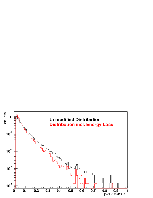
Fig. 1.7: Fragmentation functions of simulated 100 GeV jets for two different cases: the black histogram shows the fragmentation function for a sample of unmodified 100 GeV PYTHIA jets. The red histogram shows the fragmentation function of a sample of jets which have undergone energy-loss due to the medium as modeled by the superposition of a 20 GeV PYTHIA jet on a 80 GeV PYTHIA jet after [27] from [30].

1.2.2 Jets at RHIC

There are four heavy-ion experiments at RHIC which have studied Au+Au collisions at three center-of-mass energies, $\sqrt{s_{NN}}=130$ GeV, $\sqrt{s_{NN}}=200$ GeV and $\sqrt{s_{NN}}=62.4$ GeV. The experiments, in increasing order of collaboration size, are: BRAHMS (Broad Range Hadron Magnetic Spectrometers Experiment at RHIC), PHOBOS, PHENIX (Pioneering High Energy Nuclear Interaction Experiment) and STAR (Solenoidal Tracker at RHIC). Details of all RHIC experiments can be found in [31].

Evidence for jet energy loss has been reported by all four of the RHIC experiments. Three main pieces of evidence exist to support this, namely, the increasing suppression of the number of high-$p_{T}$ hadrons with increasing centrality in Au+Au events when compared to p+p events, [32, 33, 34], see Fig 1.8, the disappearance of away-side correlations in central Au+Au collisions compared to p+p collisions [35], and the d+Au results [36, 37] which allow discrimination between initial and final state effects.

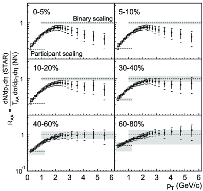
Fig. 1.8: $R_{AA}(p_{T})$ as a function of centrality. The dashed lines show scaling with $\langle N_{bin}\rangle$ and $\langle N_{part}\rangle$ and the gray bands show the systematic uncertainties. From [32].

Fig. 1.8 from the STAR experiment shows the nuclear modification factor, $R_{AA}$, defined as the ratio of the inclusive momentum spectrum of charged hadrons from Au+Au events to a p+p reference spectrum scaled to account for the nuclear geometry. The different panels show the evolution of $R_{AA}$ as a function of collision centrality. It is expected that the number of hard processes in an event scales with the average number of binary collisions $\langle N_{bin}\rangle$, in the absence of nuclear effects, which should result in $R_{AA}=1$ over a threshold defined by $p_{Thard}\approx 2$ GeV/$c$. Fig. 1.8 shows that there is a suppression from the expected value of unity which increases as a function of centrality. This result is consistent with jet energy loss in a dense medium although from these results alone, it cannot be determined whether the suppression is due to initial or final state interactions. Similar results were obtained by the PHENIX experiment [34].

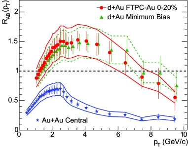
Fig. 1.9: $R_{AB}(p_{T})$ for central and minimum bias d+Au collisions and central Au+Au collisions at STAR. For clarity the d+Au minimum bias data are displaced to the right. From [36].

Fig. 1.9 shows the nuclear modification factor for central Au+Au events ($R_{AA}$) and d+Au events ($R_{AB}$) at $\sqrt{s_{NN}}=200$ GeV as measured by the STAR experiment [36]. It can be seen that the inclusive hadron yield in d+Au events is enhanced relative to p+p events which is the opposite behaviour to Au+Au collisions. Due to the small size of the system created in a d+Au collision (cannot be geometrically bigger than the size of the deuteron) it is not expected that a dense medium is formed in these collisions. Therefore, d+Au collisions can be used as a control experiment to probe initial state effects. From the lack of suppression of high-$p_{T}$ particles in d+Au collisions, it can be concluded that the suppression is due to final state effects in Au+Au collisions. Consistent results were reported by the PHENIX experiment in [37].

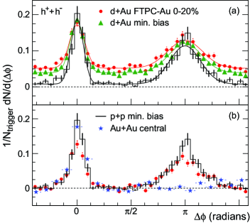
Fig. 1.10: Top panel: Two-particle azimuthal distributions for central (circles) and minimum bias (triangles) d+Au collisions compared to p+p collisions (solid line histogram). Bottom panel: Two-particle azimuthal distributions for central Au+Au collisions (stars) compared to central d+Au collisions (circles) and p+p collisions (solid line histogram). From [36].

The two-particle azimuthal distribution for central and minimum bias d+Au collisions as measured by the STAR experiment is shown in the top panel of Fig. 1.10 taken from [36]. The distribution is obtained by measuring charged hadrons around a high-$p_{T}$ trigger particle ($\Delta\phi\sim 0$) and at $180^{\rm{o}}$ from the trigger particle ($\Delta\phi\sim\pi$). In Fig. 1.10, the histogram indicates the case for p+p minimum bias collisions. The d+Au data show a near-side peak at $\Delta\phi\sim 0$ from the leading particle and an away-side peak at $\Delta\phi\sim\pi$ from the leading particle which is very similar to that of p+p collisions and consistent with di-jet production. This is different to the azimuthal distributions for central Au+Au collisions as shown in the lower panel of Fig. 1.10 where there is a clear peak in the Au+Au distribution on the near-side and a large suppression on the away-side resulting in a flat distribution.

Therefore the difference in the $R_{AB}$ and azimuthal distributions between d+Au collisions and central Au+Au collisions rules out that the suppression of high-$p_{T}$ hadrons be attributed to initial state effects: the suppression is due to final state effects produced in central Au+Au collisions.

Jet-like correlations in central Au+Au collisions have been reconstructed on a statistical basis by the STAR collaboration [38]. This is done by correlating charged hadrons in a certain energy range with a high-$p_{T}$ trigger particle. The momentum distributions for the charged hadrons on the near-side ($\Delta\phi\sim$ 0), with respect to the trigger particle, are reported to be similar to those from p+p collisions while the away-side ($\Delta\phi\sim$ $\pi$) distributions (opposite in azimuth to the trigger particle) are shifted to lower $p_{T}$ compared to the p+p case, another indication of jet energy loss. However, due to the small signal-to-background ratio and large fluctuations in the high-multiplicity Au+Au collisions, jets in heavy-ion collisions cannot be reconstructed on an event-by-event basis at RHIC, only statistically. Thus it is not yet possible at RHIC to measure jet energies and directions in heavy-ion collisions on an event-by-event basis.

1.2.3 Jets at LHC

The Large Hadron Collider (LHC) at CERN will be able to collide Pb ions at centre-of-mass energies of $\sqrt{s_{NN}}=5.5$ TeV. The dedicated heavy-ion experiment, ALICE (A Large Ion Collider Experiment) at the LHC, has been designed to measure observables both in the soft and hard physics regimes. The predicted cross-sections for hard processes at the LHC are much higher than at RHIC energies as shown in Fig. 1.11 from [39].

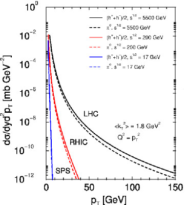
Fig. 1.11: Cross-sections for charged hadron and neutral pion production calculated using pQCD for different collision energies. From [39].

The predicted particle multiplicities for LHC follow a slow growth trend [40] from SPS and RHIC and amount to a factor of $\sim$4 greater than at RHIC, leading to an expected multiplicity of $dN_{ch}/dy=$ 2 500 as shown in Fig. 1.12. This is not the case for hard probes, for example, the cross-section for 30 GeV jets is $\sim$7 000 times higher at LHC than at RHIC [39]). Therefore, hard observables will be able to be measured above the soft-background more easily at the LHC than at RHIC.

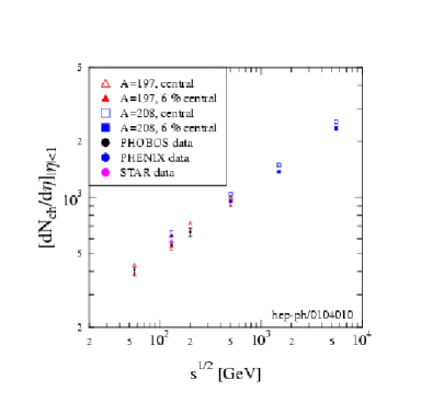
Fig. 1.12: Charged particle multiplicity averaged over an interval of $-1<\eta<1$ as a function of collision energy. Experimental data from RHIC experiments are also plotted. From [40].

1.2.4 Jet Studies at ALICE

With the predicted large cross-sections for jet production at LHC, ALICE will be able to study jets over a very broad energy range (from $\sim$5 GeV to 250 GeV). Monte Carlo simulations have shown that Pb+Pb events at top LHC energies contain a very large number of low energy ($E_{T}<20$ GeV) jets which can be studied using particle correlation techniques [41]. The number of produced jets decreases with $p_{T}$ and fewer high energy jets are expected ($\sim$100 000 jets with $E_{T}>$ 100 GeV within the experimental acceptance per year of ALICE Pb+Pb running). The high-$p_{T}$ jets will be reconstructed on an event-by-event basis.

Information from both the high-resolution tracking detectors (Inner Tracking System (ITS) and Time-Projection Chamber (TPC)) and the Electromagnetic Calorimeter (EMCal) will be used to reconstruct jets. The EMCal will function as a fast jet trigger and will increase the yield of reconstructed jet events by a factor of $\sim$200 [42]. (The TPC cannot be used as a jet trigger due to its drift time of $\sim$90 $\mu$s [43].)

The energy and direction of the jets will be measured using a combination of information from the ALICE tracking detectors (TPC, ITS) and the EMCal. Thus both the charged and neutral energy components of the jets will be recorded. The jet energy resolution, obtained using the combined detector information, is expected to be significantly improved compared to that obtained from using information from only one detector.

The motivation behind jet studies at ALICE is to investigate properties of the medium produced in Pb+Pb collisions at $\sqrt{s_{NN}}=5.5$ TeV. This will be achieved through measuring medium-induced modifications to the Pb+Pb jet fragmentation functions compared to the p+p case.

Precise measurement of the jet fragmentation functions at ALICE will involve several steps. Accurate measurement of the jet energy, jet axis and momentum distribution of the jet hadrons on an event-by-event basis will be required. The raw jet energy spectrum will then be compiled from the measured jet energies. However, this raw energy spectrum will be smeared in energy due to detector effects and resolution effects caused by the fluctuating background in Pb+Pb collisions. It will then be necessary to deconvolute these effects (for example using the method in [44]) in order to extract the true jet energy spectrum and enable comparison with p+p results, before analysing the fragmentation functions.

1.2.5 Thesis Scope

The focus of this thesis is the development of a jet-finding algorithm for heavy-ion collisions, based on the UA1 approach [45], used in p+p collisions, in order to reconstruct jet energies and directions accurately and efficiently on an event-by-event basis. Modifications are included to take into account, and correct for, the fact that in heavy-ion collisions at LHC energies, the background particle multiplicities and energy fluctuations from the ‘underlying event’ are much greater than in p+p collisions. This is the first attempt at event-by-event full jet reconstruction in heavy-ion collisions.

Deconvolution of the jet energy spectrum and measurement of jet fragmentation functions are beyond the scope of this thesis.

1.3 ALICE Experiment Overview

The ALICE detector is currently under construction within a cavern 40 m underground at Intersection Point 2 of the LHC at CERN [43]. It has been designed to detect hadrons, leptons and photons over a broad momentum range (100 MeV/$c$$<$$p_{T}$$<$100 GeV/$c$) in an environment with charged particle multiplicities of up to 8000 per unit of rapidity at central rapidities. The layout of the ALICE apparatus with its various detectors, is shown in Fig. 1.13 from [46].

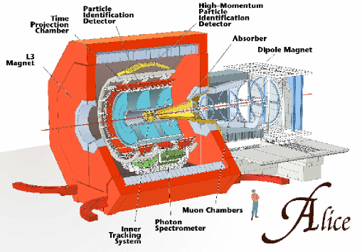
Fig. 1.13: Diagram showing ALICE detector and the positions of the various detectors. The electromagnetic calorimeter is not shown in this picture. From [46].

Most of the ALICE detectors in Fig. 1.13, with the exception of the muon spectrometer, are positioned at midrapidity (-0.9$\leq\eta\leq$0.9) within the large L3 magnet which is designed to provide a magnetic field of 0.5 T to enable measurement of particle momenta and identities by the various detectors. The magnet is 12 m long and has a radius of 5 m. Starting at the interaction vertex and proceeding outwards, the ALICE central detector system includes the:

• Inner Tracking System (ITS) consisting of six layers of high-resolution silicon tracking detectors,

• Time-Projection Chamber (TPC) which is the primary tracking detector in ALICE,

• Transition Radiation Detector (TRD) for the identification of electrons,

• Time Of Flight Detector (TOF) for particle identification,

• High-Momentum Particle Identification Detector (HMPID) which is an array of ring-imaging Cherenkov detectors for high-momentum particle identification,

• Photon Spectrometer (PHOS) which consists of a small area lead-glass crystal electromagnetic calorimeter (-0.12$<\eta<$0.12, $\Delta\phi=100^{\rm{o}}$) (for detection of photons and neutral mesons through their decay into photons) and a charged particle detector (CPV) which acts as a veto detector for charged particles which deposit energy in the calorimeter [47],

• Proposed Electromagnetic Calorimeter (EMCal) (not shown here) which is a large area (-0.7$<\eta<$0.7, $\Delta\phi=120^{\rm{o}}$) lead-scintillator sampling calorimeter.

The Muon Spectrometer covers forward rapidity. It consists of a dipole magnet, tracking stations, a muon filter, trigger stations and an absorber close to the vertex which acts as a shield for the spectrometer. Other detectors which are not shown in Fig. 1.13 include a Photon Multiplicity Detector (PMD) which counts photons and a Forward Multiplicity Detector (FMD). Two Zero Degree Calorimeters (ZDC), positioned at $0^{\rm{o}}$ about 90 m from the interaction vertex, will be used to measure event centrality.

The main ALICE tracking detector, the TPC, covers an area between -0.9$<\eta<$0.9 and has full azimuthal coverage. The tracking efficiency of the TPC has been tested using simulations of Pb+Pb collisions with charged particle multiplicities of $dN_{ch}/d\eta=$ 8 000 resulting in efficiencies of greater than $90\%$ [43]. The momentum resolution of the TPC for tracks with 100 MeV/$c$$<p_{T}<$1 GeV/$c$ is $\sim$1-2$\%$ [43]. For tracks with $p_{T}>1$GeV/$c$, the TPC can be used in combination with the other tracking detectors for optimal resolution as shown in Fig. 1.14 from [48]. For example for 30 GeV tracks, the addition of further tracking information from the ITS and TRD, in addition to the TPC, improves the momentum resolution from $\sim$21$\%$ (TPC only) to $\sim$5$\%$.

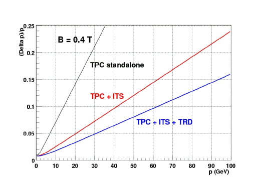
Fig. 1.14: Momentum resolution of the the ALICE tracking detectors. The black line shows the resolution using the TPC only, the red line shows resolution using TPC + ITS detectors and the blue line shows the improvement when using TPC, ITS and TRD detectors. From [48].

The electromagnetic calorimeter (EMCal) will measure the neutral component of jet energy as discussed in Section 1.2.4. It will also be used to trigger on jets. The EMCal is a Pb-scintillator sampling calorimeter which covers an area of -0.7$<\eta<$0.7 and $60^{\rm{o}}<\phi<180^{\rm{o}}$, see Fig. 1.15 [46]. It consists of 12 super-modules which altogether make up a total of $114(\eta)$ x $168(\phi)=19152$ towers with projective geometry. From simulations, the EMCal energy resolution is $\sim$15$\%/\sqrt{E}$ [42].

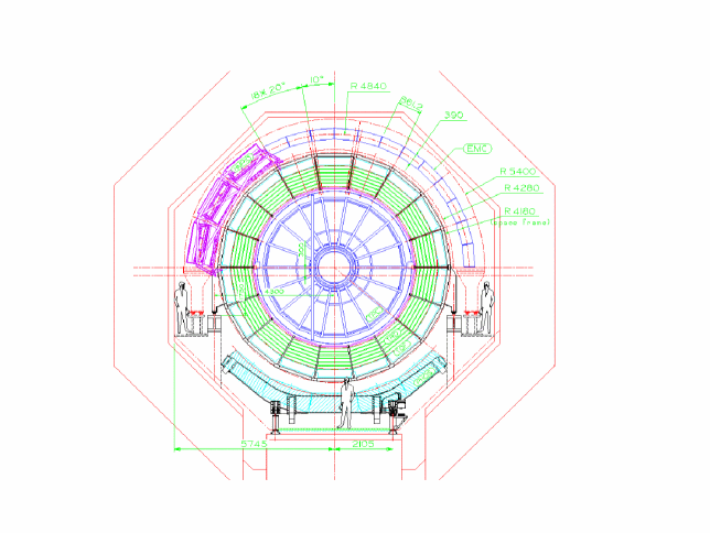
Fig. 1.15: Technical drawing of cross-section through ALICE. The electromagnetic calorimeter is shown in the outermost layer lying just below the octagonal magnet and spanning from $0^{\rm{o}}-120^{\rm{o}}$ (where the diagram is looking towards positive $z$ here). From [46].

Chapter 2 Reconstructing Jets at LHC Energies

2.1 Current Jet Finding Methods

Jets have been studied for many years in the field of high energy physics at hadron-hadron colliders and $e^{+}e^{-}$ colliders and various algorithms have been developed to identify them and measure their properties. With the high energies used to collide heavy ions at the Relativistic Heavy Ion Collider (RHIC), it has recently become possible to study jets experimentally in heavy-ion collisions as well.

2.1.1 Methods Used in High-Energy Physics

The algorithms used to find and reconstruct jets were first developed in the field of high-energy physics. Jet production cross-sections can be predicted using pQCD calculations. Experimental measurements of the jet cross sections can test the predictions. Jet cross-sections have been measured at both $e^{+}e^{-}$ and hadron-hadron colliders. However, due to the different event structures in the two cases, different jet definitions and algorithms to reconstruct them, have been developed [49]. The aim of both however, is to provide a mapping between the observed high-energy hadrons and the initial state energetic partons which were involved in the hard scattering.

In $e^{+}$+$e^{-}$ collisions, at the lowest order the initial state is purely electromagnetic and therefore all the final state hadrons are due to the annihilation process giving rise to a virtual photon which splits into a $q\overline{q}$ pair. In hadron-hadron collisions there are a large number of initial state partons but generally only one parton from each of the incident hadrons is involved in a hard scattering. Therefore, out of all the final state hadrons produced in the collision, a fraction can be associated with the hard scattering process and the rest are considered part of the ‘underlying event’. The final state hadrons forming the ‘underlying event’ contribution are due to soft interactions and rescattering between the remaining partons in the incident hadrons. Another difference in the event structures is that in hadron-hadron collisions, the partons involved in the hard scattering process produce radiation in the form of initial state bremsstrahlung and this radiation combined with the underlying event, produces the ‘beam jets’ observed at hadron colliders.

The Cone Jet Algorithm

A cone jet definition, originally defined in [50] has been used to reconstruct jets in hadron-hadron collisions [51, 52]. A cone jet is defined as a group of particles whose 3-momenta all lie within a cone of a certain angular size. ‘Beam jets’ are suppressed by this definition because only a fraction of the low-$p_{T}$ ‘beam jet’ hadrons will fall inside the cone of a high-$p_{T}$ jet. Analytically, a cone algorithm groups together all particles, $i$, whose trajectories lie within a cone, $C$, of a certain radius, $R$, in ($\eta$,$\phi$)-space where

$$\sqrt{(\eta^{i}-\eta^{C})^{2}+(\phi^{i}-\phi^{C})^{2}}\leq R.$$ (2.1)

Experimentally, since the data is usually in the form of output from electromagnetic or hadronic calorimeters, or a combination of both, the cone is projected to two dimensions in the form of a circle of radius $R$, in ($\eta$, $\phi$)-space where the calorimeter tower positions can be used to represent the particle trajectories. Cone algorithm iterations begin with a trial cone centre around a seed tower, usually with energy above some threshold (so-called ‘seed’ energy). The energy of particles inside the cone is used to calculate the $E_{T}$-weighted centroid of the cone which then becomes the new cone centre. The same process is repeated until a ‘stable’ cone centre (when the change in position of the centroid between successive iterations is small or below a chosen parameter) is found. The particles falling inside the stable cone are then classified as part of the jet. A recombination scheme, for example the original Snowmass scheme [53], is defined to reconstruct the transverse energy and direction of the cone jet as follows:

$$E^{J}_{T} = \sum_{i\subset J=C}E^{i}_{T}=E^{C}_{T}$$ (2.2)

$$\eta^{J} = \frac{1}{E^{J}_{T}}\sum_{i\subset J=C}E^{i}_{T}\eta^{i}$$ (2.3)

$$\phi^{J} = \frac{1}{E^{J}_{T}}\sum_{i\subset J=C}E^{i}_{T}\phi^{i}$$ (2.4)

A number of corrections are applied to the reconstructed jet energy to take into account the non-uniform response of different types of calorimeters and edges and gaps in the calorimeters. Attention is also given to the non-linear response of the calorimeter to low momentum particles. Further corrections involve a subtraction of the estimated energy from the ‘underlying event’ and an addition to take into account the jet energy that lies outside the chosen cone radius [54, 55].

Fig. 2.1 shows the flow chart representation of the cone algorithm used at the CDF experiment [51]. This cone algorithm does not take into account that jets may overlap and thus one calorimeter tower may be included in more than one final jet. In order to take care of this problem, further ‘splitting’ and ‘merging’ algorithms have been developed [51]. The choice of cone radius differs from experiment to experiment, for example, $R=1.0$ was originally used at UA1 [52] but smaller cone sizes of $R=0.4,0.7$ have been used at CDF and DØ, [51, 56, 57]. A discussion of the choice and optimisation of algorithm parameters is in section 3.2.

[rowsep=0.5cm,colsep=0.8cm]

Fig. 2.1: Cone jet finding algorithm used at the Tevatron at Fermilab, from [51].

The $k_{T}$ Algorithm

For the $e^{+}$+$e^{-}$ case, the commonly used algorithm is called the $k_{T}$ algorithm. This method successively groups sets of particles with ‘nearby’ momenta into larger sets of particles which are then classified as jets [49]. The jets defined this way typically do not have regular shapes compared to the cone jets defined in the cone jet algorithm but with this definition there is no problem of overlapping jets because each particle (or calorimeter tower) is uniquely associated with one jet. The $k_{T}$ algorithm has also been adapted for hadron-hadron collisions [51, 49]. In the $k_{T}$ algorithm used at the Tevatron, [51], ‘preclusters’ of grouped particles or calorimeter towers are formed (similar to finding towers with energy above some ‘seed’ energy in the cone algorithm). Iterating over all preclusters until there are none left resulted in each precluster having a four-momentum vector assigned to it where

$$(E,\textbf{p})=E(1,\cos\phi\sin\theta,\sin\phi\sin\theta,\cos\theta)$$ (2.5)

and $E$ is the energy of the precluster, $\theta$ is the polar angle with respect to the beam axis, and $\phi$ is the azimuthal angle. Thus the square of the precluster’s momentum and its rapidity can be calculated:

$$p_{T}^{2} = p_{x}^{2}+p_{y}^{2}$$ (2.6)

$$y = \frac{1}{2}\ln\frac{E+p_{z}}{E-p_{z}}.$$ (2.7)

Next, for each precluster:

$$d_{i}=p_{T,i}^{2}$$ (2.8)

and for each pair of preclusters where $i\neq j$

$$d_{ij}=\min(p_{T,i}^{2},p_{T,j}^{2})\frac{(y_{i}-y_{j})^{2}+(\phi_{i}-\phi_{j})^{2}}{D^{2}}$$ (2.9)

is defined. $D\approx 1$ and is one of the algorithm parameters. The minimum of all the $d_{i}$ and $d_{i,j}$ is then found and labeled $d_{min}$. If $d_{min}$ was originally a $d_{ij}$ then preclusters $i$ and $j$ are merged to form a new precluster with

$$E_{ij} = E_{i}+E_{j}$$ (2.10)

$$p_{ij} = p_{i}+p_{j}.$$ (2.11)

Otherwise, if $d_{min}$ is a $d_{i}$, then the precluster is classified as ‘not mergeable’ and is added to the list of jets. A flowchart representation of the algorithm is shown in Fig. 2.2 taken from [51].

[rowsep=0.5cm,colsep=0.8cm] &

Fig. 2.2: $k_{T}$ jet finding algorithm used at the Tevatron at Fermilab from [51].

Energy Summation Methods

The jets resulting from the fragmentation of hard scattered partons are composed of charged and neutral hadrons and their hadronic, leptonic and photonic decay products i.e.

$$E_{Jet}=\sum{E_{Charged}}+\sum{E_{\gamma,Leptons}}+\sum{E_{Neutral}}.$$ (2.12)

For optimal jet energy resolution, the various components of the jets need to be taken into account in the jet finding algorithms. Therefore, in order to measure full jet energies experimentally, detectors are needed which can measure the energies of the different types of particles. Usually, calorimetry (both electromagnetic and hadronic) information has been used as input to jet finding algorithms [51, 52]. However, some particle physics experiments, including ALEPH at LEP [58] and CDF at the Tevatron [54], have also included tracking information, resulting in much improved jet energy resolution. In the case of CDF, each track is associated with a calorimeter tower and thus the combination of calorimetric and tracking information is used in jet finding. A process has been devised to take care of double counting the energy from particles that leave tracks and also deposit energy in the calorimeters. The improvements in jet energy resolution at CDF due to the inclusion of tracking information in addition to shower maximum and calorimetry information is shown in Fig. 2.3 from [59].

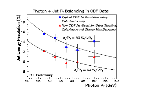
Fig. 2.3: Jet energy resolution as a function of the photon energy in the sample of $\gamma$-jet events measured [59].

It is also possible to measure certain components of jets, for example charged particle jets have been measured at CDF [56]. Charged particle jets are defined in [56] as clusters of charged particles within circular regions of ($\eta$,$\phi$)-space of radius $R=\sqrt{(\Delta\eta)^{2}+(\Delta\phi)^{2}}=0.7$. In contrast to using calorimeter data, in this case a cone jet algorithm was used on tracking data from the Central Tracking Chamber (CTC).

2.1.2 Methods Used in Heavy-Ion Physics

In the field of heavy-ion physics, jets are a relatively new observable. At the lower energies of previous heavy-ion experiments, the cross-sections for hard processes and jet production were low and it was also difficult to identify low-energy jets above the background in the events [35, 60]. However, at RHIC, with the increase in collision energy, the jet cross-section has increased relative to previous heavy-ion experiments and jet-like signals have been observed at the STAR and PHENIX experiments by using a statistical two-particle angular correlation method. Angular correlation methods were also used in the past for p+$\overline{\rm{p}}$ collisions, prior to the development of jet finding algorithms, to confirm the existence of parton hard scattering and fragmentation into hadrons [61]. When a hard parton fragments, the resulting high-$p_{T}$ hadrons are correlated at small $\Delta\eta,\Delta\phi$ [61].

At the STAR experiment at RHIC, for example, jet-like correlations have been measured by constructing the azimuthal correlations of high-$p_{T}$ charged particles detected in the STAR TPC [60]. Events containing a trigger particle with transverse momentum in a chosen range $trig_{min}<p_{T}(trig)<trig_{max}$ and within a chosen region of pseudorapidity $|\eta|<x$ are selected. For these events, the relative azimuthal distribution of other charged tracks with $track_{min}<p_{T}<trig_{min}$ and in the same $|\eta|$-range, normalised by the number of high-$p_{T}$ trigger particles, is constructed. The correlation function is given by

$$\frac{1}{N_{trigger}}\frac{dN}{d(\Delta\phi)}\equiv\frac{1}{N_{trigger}}\frac{1}{\epsilon}\int{d\Delta\eta N(\Delta\phi,\Delta\eta)}$$ (2.13)

where $N_{trigger}$ is the number of tracks fulfilling the trigger requirement, $\epsilon$ is the single track efficiency, and $N(\Delta\eta,\Delta\phi)$ is the number of observed pairs of hadrons as a function of relative pseudorapidity, $\Delta\eta$, and relative azimuth, $\Delta\phi$.

Thus, so far at heavy-ion collision experiments, jets are found on a statistical basis and the jet properties such as jet energy and direction have not been able to be measured on an event-by-event basis in heavy-ion collisions.

2.2 Specifications for a Jet Finding Algorithm for Use at ALICE

At ALICE, the purpose (as discussed in Section 1.2.4) of finding and measuring jets is to be able to measure the jet fragmentation functions and thus be able to infer properties of the medium produced in the heavy-ion collision. The fragmentation function $D(z)$ was defined in equation (1.1) where $z=p_{L}/E_{Tjet}$. Replacing $z$ with the quantity $p_{P}/E_{Tjet}$, where $p_{P}$ is the momentum component of a jet particle in the direction perpendicular to the jet axis, is also of interest when looking for modifications of jet fragmentation functions due to jet-quenching. Therefore, to measure accurately the jet fragmentation functions, the jet direction, which approximates the original parton direction, and the jet transverse energy, which approximates the scattered parton transverse energy, need to be measured. In order to be able to make a meaningful measurement of the fragmentation functions, a large, unbiased sample of jets is needed.

The two-particle correlation methods used currently at heavy-ion experiments are not appropriate in this case since they are used to find the existence of jets but do not measure jet energies or directions accurately. Also, by choosing only events that satisfy a high-$p_{T}$ charged particle trigger, events where jets are led by neutral particles can be excluded. In addition, the trigger requirement biases the jet selection to jets which fragment primarily to a single high-$p_{T}$ leading particle, biasing the measured fragmentation function.

2.3 Proposed Jet Finding Algorithm for Use at ALICE

At the ALICE experiment, the concept of using a combination of data from multiple detectors to find jets will be applied, similarly to what has been done in particle physics experiments[54, 58]. The ALICE TPC will provide highly efficient particle tracking capabilities (Section 1.3). The EMCal will act as a fast jet trigger as well as providing calorimetric data. Since the cross-section for jet production at the LHC is expected to be much higher than at RHIC (see Section 1.2) and the ratio of jet signal to background to be much better, the use of algorithms similar to those used in particle physics becomes more viable. However, some modifications need to be implemented to take care of the large background signal and the underlying event-by-event fluctuations.

The algorithm proposed here is based on a version of the UA1 cone jet algorithm [45]. Further modifications have been made to take into account the background characteristics expected at the LHC. In its final version, it is very similar to the cone algorithm presented in Section 2.1.1. The cone algorithm was chosen as a starting point for jet finding in heavy-ion collisions because it has been successfully used in hadron-hadron collisions. With the very high multiplicity backgrounds and the signal to background ratios expected in heavy-ion collisions at the LHC, adapting a $k_{T}$ algorithm would be more difficult.

The ALICE Cone Jet Algorithm

The ALICE cone jet algorithm follows the same main steps as the particle physics cone jet algorithm already discussed and a detailed flow chart representation of the algorithm is shown in Fig. 2.4.

[rowsep=0.5cm,colsep=0.8cm]

Fig. 2.4: Modified cone algorithm for the heavy-ion case at ALICE at the LHC.

The main difference between the two algorithms is the addition of an iteration (Box 2 in Fig. 2.4) to ensure more accurate calculation of the background or ‘underlying event’ on an event-by-event basis. The data input to the algorithm are a combination of calorimeter data from the EMCal and tracking data with transverse energies $E_{T}$ ($\approx p_{T}$) projected onto a grid in ($\eta,\phi$)-space with cells of the same granularity as the EMCal towers.

Towers are then sorted in decreasing order of $E_{T}$ and the average background energy per tower, $E_{BG_{Ave}}$ is calculated. Iterating over all towers, if the tower energy after background subtraction is greater than a set seed energy, $JetESeed$, and if the tower is not already part of a jet, then iterations begin to calculate the centroid of the jet cone. Centroid iterations continue until the distance between the current centroid and the centroid from the previous iteration is less than $0.05R$ and the distance between the initiator tower and the calculated centroid is smaller than $0.15R$. (These parameters are tunable and here the choice of parameters in [45] is followed.) Once the centroid is found, the jet energy $E_{T}^{J}$, is calculated by summing the energy of each tower, after background subtraction, that is within the cone radius, $R=\sqrt{(\eta^{i}-\eta^{C})^{2}+(\phi^{i}-\phi^{C})^{2}}$. If the calculated jet energy is greater than a minimum value, $MinJetEt$, then the jet is classified as valid and added to the list of jets. The scheme used to calculate the jet cone centroid position in ($\eta,\phi$)-space and the jet transverse energy is the same as the original Snowmass scheme [53] used in particle physics as given by equations 2.2-2.4. There are three parameters, namely the cone radius $R$, the jet seed energy, $JetESeed$, and the minimum allowed jet energy, $MinJetEt$, that need to be optimised to produce the optimal jet energy resolution and jet finding efficiency. The algorithm can also be made into a seedless algorithm by setting the $JetESeed=0$. The optimisation analysis is presented in Chapter 3 and results using the optimised parameters are discussed in Chapter 4.

2.4 Simulation of jets in the ALICE framework

Two Monte Carlo event generators were used to simulate the data for high-$p_{T}$ jets in heavy-ion collisions at $\sqrt{s_{NN}}=5.5$ TeV at ALICE [62]. Within the ALICE software framework, namely AliRoot [63], PYTHIA 6.2 [28] was used to simulate the high-$p_{T}$ jets and HIJING 1.36 [29] was used to simulate the high multiplicity background or ‘underlying event’. In order to simulate a jet event in a heavy-ion collision, a PYTHIA p+p jet event was superimposed on a HIJING Pb+Pb event. The passage of particles through the materials of the ALICE detectors was simulated using GEANT3 [64]. The EMCal response was simulated using GEANT3 and a parameterised detector response was used for charged tracks in the ALICE tracking system.

Simulations Note

Immediately prior to the submission of this thesis, it was found that Birks’ formula [65], describing the deviation from a linear response of the light emitted due to the energy deposited by a particle in the scintillator, had not been applied in the simulations [62]. The deviations for heavier, higher ionising particles are larger than for lighter particles. The light response of the scintillator is dependent on the type of particle depositing energy, the amount of energy deposited and the ionisation of the particle. Preliminary simulations [67] have shown that this is a small effect ($<10\%$) and is not expected to have a large impact on the analysis and results presented in this thesis.

2.4.1 PYTHIA Events

PYTHIA is a Monte Carlo event generator which generates high energy physics events [28]. The model has been tuned to reproduce the same detail and results as obtained from experimental measurements. PYTHIA includes QCD and QED as well as other theories beyond the standard model. In this case PYTHIA was used to generate jets from hard scatterings in p+p collisions at $\sqrt{s_{NN}}=5.5$ TeV. Certain nominal jet energies were chosen at which to simulate jets so that the results produced by the algorithm could be reconciled with the input jet energies. Jets were generated within narrow windows of $\pm 2$ GeV around the nominal energies of 30 GeV, 50 GeV, 75 GeV, and 100 GeV. Since the statistical error $\sigma\sim$1$/\sqrt{n}$ where $n$ is the number of events, 10 000 events were generated at each energy to keep the statistical error to the $1\%$ level. A condition applied to the events ensured that at least one jet was pointing towards the fiducial volume of the EMCal. Initial and final state radiation were included because the simulated interaction was at a high energy where the emission of hard gluons plays a large role, relative to fragmentation, in determining the structure of events [66]. Initial state radiation is the radiation of gluons from a parton before it interacts in a hard scattering and final state radiation describes the radiation of gluons from the hard scattered parton before it fragments into a jet. More specifically, the parameters for the generation of the PYTHIA events with jets of nominal energy $x$ GeV were as follows:

• Initial state and final state gluon radiation ON

• $\sqrt{s_{NN}}=5.5\ \rm{TeV}$

• $x-2\ \rm{GeV}$ $<E_{T_{Jet}}<x+2\ \rm{GeV}$

• $\eta_{Jet}<|0.3|$

• $75^{\rm{o}}<\phi_{Jet}<165^{\rm{o}}$

• Structure function is GRVLO98

• $x\ \rm{GeV}$ $<p_{T_{HardScattering}}<x+0.1\ \rm{GeV}$

• All decay types ON

2.4.2 HIJING Events

HIJING (Heavy Ion Jet Interaction Generator) is a Monte Carlo event generator for A+A collisions [29]. It uses a perturbative QCD approach, based on PYTHIA, to model multiple jet production in the collisions. HIJING also includes the production of multiple mini-jets which dominate events with high multiplicities [29] and which can lead to correlations in transverse momentum observables and fluctuation enhancements. HIJING therefore attempts to model the observed event-by-event fluctuations in the ‘underlying event’ in heavy-ion collisions.

Two types of HIJING events were simulated, namely central HIJING events and parameterised HIJING events. Parameterised HIJING events are a parameterised version of real HIJING events containing only pions and kaons sampled from the $p_{T}$ and $\eta$ distributions of particles in real HIJING. The multiplicity of the events can be set to any $dN/dy$ and for the purpose of this thesis, a multiplicity of $dN/dy=$ 4 000 was used and the event type will be referred to as parameterised HIJING 4000 from now on. As shown in Fig. 1.12, the predicted charged particle multiplicity for central Pb+Pb collisions at $\sqrt{s_{NN}}=5.5$ TeV is $\sim$2 500. Therefore, in order to be conservative in the simulations, a multiplicity of 4 000 was simulated in the events. An advantage of using parameterised HIJING events is that they do not require detailed calculations to be performed since they sample different distributions and the computing time required is relatively short. However, since these events are a parameterisation, they do not accurately simulate the event-by-event background fluctuations as seen in full HIJING simulations and real data. Fig. 2.5 shows the energy distributions in a grid in ($\eta,\phi$)-space with cells of the same granularity as the EMCal from full central HIJING events (shown in red) and parameterised HIJING 4000 events (shown in green). The distributions consist of a combination of energy from charged particles leaving tracks in the TPC and which were pointing in the direction of the EMCal, and from particles which deposited energy in the EMCal. The parameterised HIJING 4000 events show a much narrower distribution than the full central HIJING events with fluctuations of the order of $6\%$ compared to the full central HIJING fluctuations which are of the order of $19\%$.

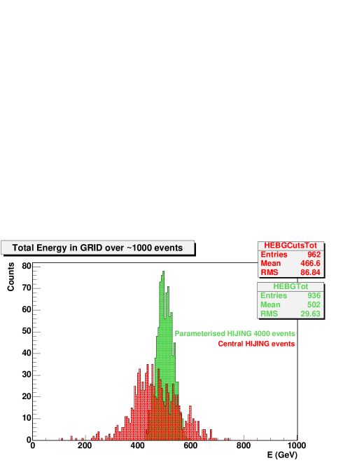
Fig. 2.5: Total GRID energy for Parameterised HIJING 4000 events (shown in green) and for Central HIJING events (shown in red).

Almost all simulations of jet events with background shown here consist of PYTHIA events mixed with full HIJING events. The cases where parameterised HIJING 4000 events are used, are clearly noted.

The full HIJING events that were simulated will be denoted ‘central HIJING’ events from now on. Multiplicity in heavy-ion collisions is proportional to the event centrality and thus the highest multiplicity events were generated in order to test the algorithm in a very conservative situation. Since full HIJING event simulations take many hours to run and have a size of the order of 400 megabytes per event, 1 000 events of this type were simulated. When performing analysis, the events were mixed randomly with the PYTHIA events. The central HIJING event generation parameters were as follows:

• $\sqrt{s_{NN}}=5.5\ \rm{TeV}$

• Jet-quenching for new LHC parameters with log(e) dependence ON
  (Special parameters from ALICE workshop 2003)

• Gluon shadowing ON

• Impact parameter $b\leq 5$ fm

• Initial state and final state radiation ON

• Decays of $\pi^{0}$, $K^{0}_{s}$, $D^{\pm}$, $\Lambda$, $\Sigma^{\pm}$ OFF

Chapter 3 Analysis

The jet data analysed in this section were simulated using PYTHIA 6.2 and HIJING 1.36 Monte Carlo event generators. The process used to reconstruct jets and a description of the optimisation of the jet finding algorithm will be described in the following sections.

3.1 Input Data and Preparation for Jet Finding

3.1.1 Jet Finding Data Preparation

Since information from both the tracking detectors and the EMCal needed to be combined for jet finding, an energy grid was created with the same fiducial range as the EMCal ($|\eta|<0.7$, $\pi/3\leq\phi\leq\pi$) and with the same number of cells as the EMCal towers ($13824=96(\eta)\times 144(\phi)$). After some data preparation (detail to follow), the grid was then filled with energy from calorimeter hits and from charged tracks from primary particles measured in the TPC that were originally pointing towards the EMCal fiducial area, see Fig. 3.1 and Fig. 3.2.

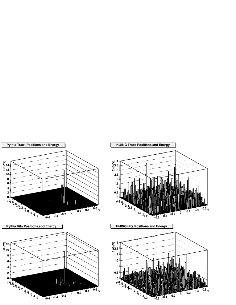
Fig. 3.1: Left hand top(bottom) plot shows the energy from PYTHIA charged tracks(hits) in the grid for a 100 GeV PYTHIA event before data preparation is performed. Right hand top(bottom) plot shows the energy from Central HIJING charged tracks(hits) in the grid before any data preparation.

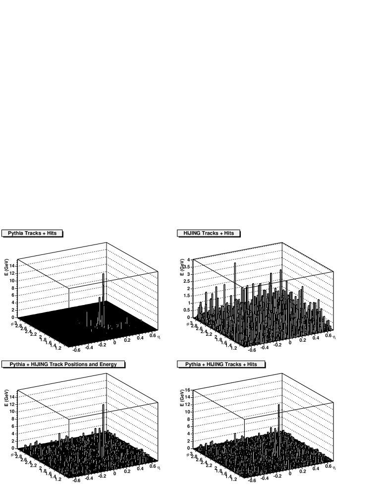
Fig. 3.2: Top left hand plot shows the energy from tracks plus hits for a 100 GeV Pythia event, top right hand plot shows the same for a Central HIJING event. Bottom left shows sum of track energies from a 100 GeV Pythia event and a Central HIJING event, while bottom right hand plot shows the sum of all track and hit energies from the 100 GeV Pythia and HIJING events.

Time cut

The first step in preparing the data for jet finding was to apply a time cut on the hits measured in the EMCal, i.e. all hits measured after 30 ns were not added to the grid. The time cut suppressed the amount of background energy measured due to backscattering in the detector. There will also be a hardware time cut implemented to do this on real data. Fig. 3.3 shows the energy deposited in the EMCal as a function of time after a collision. In all panels, the dashed vertical line indicates the time cut at 30 ns. The top left hand plot shows the source of the energy in the EMCal as a function of time where the blue histogram represents the fraction of energy deposited in the EMCal by primary particles that were originally pointing into the EMCal fiducial volume and the red histogram shows the fraction due to particles that were orginally pointing outside the EMCal fiducial volume. It can be seen that most of the energy from primary particles initially pointing in the correct direction, is deposited early while the major energy contribution after $\sim$30 ns is due to primary particles that were not pointing in the direction of the EMCal initially. The top right hand plot in Fig. 3.3 shows the ratio of the energy due to primary particles initially inside the EMCal acceptance to the energy due to primary particles outside the EMCal acceptance (i.e. the ratio of the blue histogram to the red histogram in the left hand figure). The energy due to particles orginally outside the EMCal acceptance overtakes the energy due to particles inside the acceptance range after $\sim$30 ns as can be seen by the ratio dropping below 1 around $30$ ns. The bottom plot in Fig. 3.3 shows the absolute energy deposit from the different primary particles in units of GeV as a function of time. The effect of the time cut on the energy deposited by primary particles pointing into the EMCal acceptance was to exclude $\sim$10.4$\%$ of the energy.

The time cut was found to reduce the energy measured in the grid by a factor of $\sim$1/3 and to increase the ratio of energy due to primary particles inside the EMCal acceptance to energy due to primary particles outside the EMCal acceptance to $\sim$1, see Fig. 3.3.

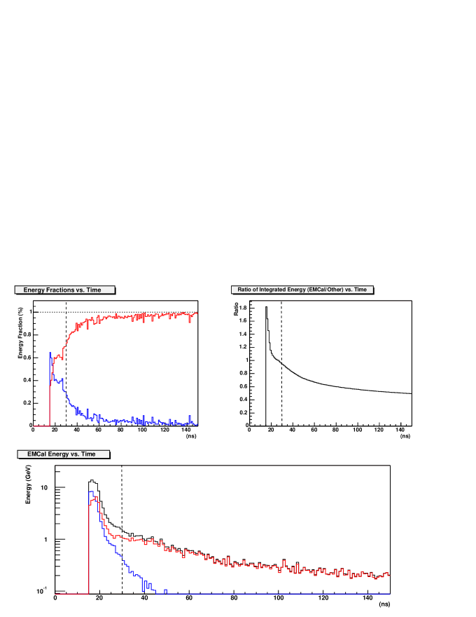
Fig. 3.3: Top left plot shows the source of the energy in the EMCal as a function of time after a collision. The blue histogram represents the energy deposited due to particles initially pointing into the EMCal fiducial volume. The red histogram shows the energy fraction due to particles that were orginally pointing outside the EMCal fiducial volume. The top right hand plot shows the ratio of the energy due to primary particles initially inside the EMCal acceptance to the energy due to primaries outside the EMCal acceptance. The bottom plot shows the energy deposited in the EMCal from the two sources as a function of time. The vertical dashed line in all plots indicates the time cut of 30 ns. From [30].

Hadron Correction

The next correction to be made was to eliminate the double counting of energy from charged hadrons measured in both the TPC and the EMCal. All charged hadrons leave tracks in the TPC and will deposit energy in the EMCal if they are within its fiducial volume. Therefore, when adding track energy and hit energy, some double counting of energy occurs. To correct for this, an average amount of energy, $\langle E_{HC}(\eta,p_{T})\rangle$, was subtracted from all the grid cells whose coordinates in ($\eta,\phi$)-space matched the direction in which a primary track was initially pointing. In order to calculate $\langle E_{HC}(\eta,p_{T})\rangle$ for each primary track, 10 000 events each were simulated for seven different particle momenta and six different $\eta$-directions, where a single charged pion was detected in both the TPC and the EMCal [30].

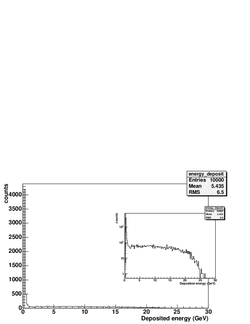
Fig. 3.4: Main plot shows the distribution of deposited energy in the EMCal from 10 000 $\pi^{+}$ each with an energy of 25 GeV and $\eta$-direction = 0.0. In this case $\langle E_{dep}\rangle=5.4$ GeV. The inset shows the same plot with a log scale. From [30].

Fig. 3.4 shows that the mean energy deposited by a 25 Gev $\pi^{+}$ in the calorimeter is 5.4 GeV. For each case of particle momentum and direction, the average energy deposited $\langle E_{dep}\rangle$ was calculated. A parameterisation of the energy deposition as a function of particle $p_{T}$ and $\eta$-direction was obtained from fitting the $\langle E_{dep}\rangle$ as a function of $\eta$ and $p_{T}$ [30]. For each charged track in the EMCal fiducial volume, $\langle E_{HC}(\eta,p_{T})\rangle$ was calculated using the parameterisation and then subtracted from the relevant grid cell.

Track $p_{T}$-cut

A further method used to reduce the background energy in the grid from the underlying event, was to perform a $p_{T}$-cut on all tracks in the grid. The average $p_{T}$ distributions for charged tracks for a jet event and background event (averaged over many events) can be seen in Fig. 3.5. The average jet track $p_{T}=2.5$ GeV/$c$ whereas the average background track $p_{T}=0.63$ GeV/$c$. Thus, a $p_{T}$-cut of $2.0$ GeV/$c$ excluded $98\%$ of background tracks and $62\%$ of jet tracks, see Fig. 3.5.

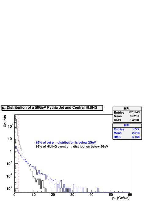
Fig. 3.5: $p_{T}$ Distributions averaged over $\sim 1000$ events for 50 GeV PYTHIA events (in blue) and Central HIJING events (in black) respectively. The dotted line indicates the $p_{T}$-cut at 2.0 GeV/$c$.

3.1.2 Study of the Characteristics of the ‘Underlying Event’

Event-by-Event Background Energy Fluctuations

The main cause of complexity in jet finding in heavy-ion collisions, is the size of the event-by-event fluctuations of energy deposited in the detectors by particles from the ‘underlying event’. Therefore a more detailed study was performed to quantify the amount, and spread, of the background energy event-by-event. The impact that a $p_{T}$-cut on the track momenta and a $30$ ns time cut on hits in the EMCal would have on the background energy distribution in the grid was also studied.

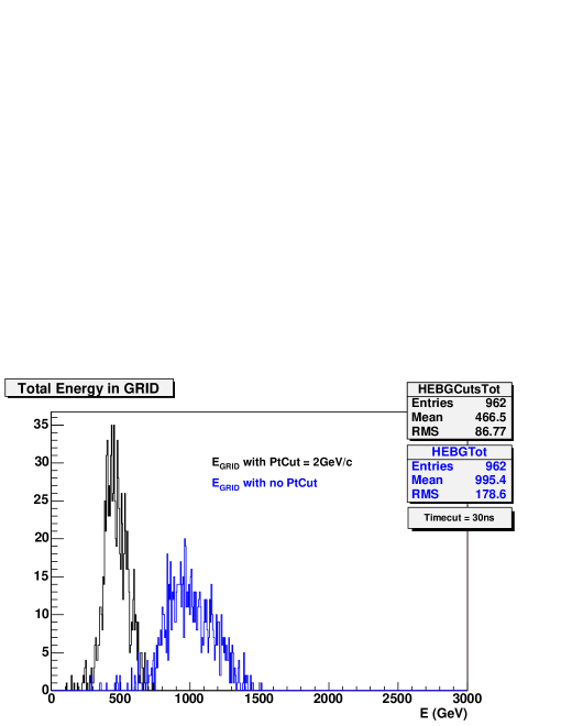
Fig. 3.6: Energy in the grid from 1 000 Central HIJING background events. Blue indicates the distribution without a $p_{T}$-cut and black indicates the resulting distribution with $p_{T}$-cut = 2 GeV.

Fig. 3.6 shows the distribution of total energy deposited in the grid for 1000 Central HIJING events with and without a $p_{T}$-cut. For both cases, a time cut of $30$ ns was applied. The mean energy deposited in the grid with a $p_{T}$-cut imposed, was 467 GeV with large event-by-event fluctuations of the order of $20\%$. The fluctuations without a $p_{T}$-cut were also of the order of $20\%$ but the mean deposited energy was 995 GeV. Thus the addition of the 2 GeV $p_{T}$-cut, while excluding $98\%$ of background tracks, reduced the background grid energy by a factor of $2$.

The effect of a $p_{T}$-cut and a time cut on the background energy as a function of cone radius $R$ was also studied. For 1 000 Central HIJING events, the amount of energy was summed within different sized cones which were randomly positioned on the grid. The results can be seen in Fig 3.7. The addition of the $p_{T}$-cut and time cut was found to reduce the absolute size of the fluctuations and the mean energy in the cone by $\sim$70$\%$ with the time cut having a larger effect ($\sim$40$\%$) than the $p_{T}$-cut ($\sim$30$\%$).

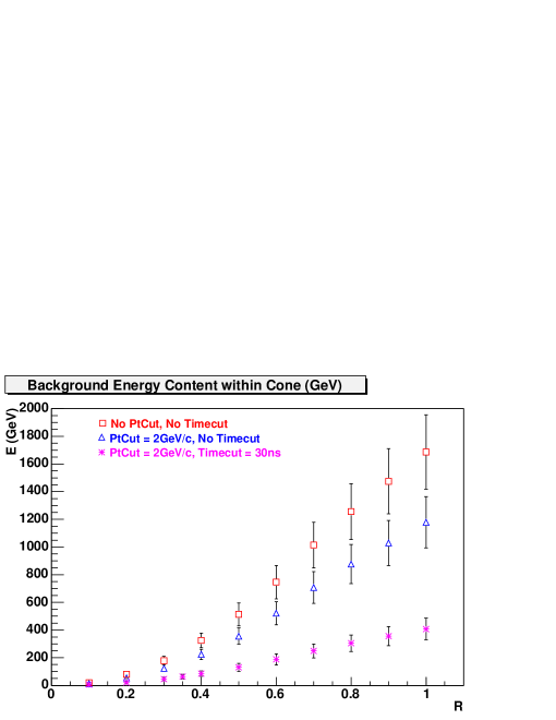
Fig. 3.7: Background energy contained within a cone as a function of cone radius, $R$. The symbols represent the mean of the distributions for set $R$ and the error bars represent the RMS for each distribution. Squares represent no $p_{T}$-cut or time cut, triangles represent $p_{T}$-cut only and stars represent $p_{T}$-cut and a time cut on the data.

The next step in the background study was to determine how the background energy contained within various cone radii, $R$, compared to the amount of jet energy contained within the same $R$. For 10 000 PYTHIA events of different energies (30 GeV, 50 GeV, 75 GeV, 100 GeV), the energy from the tracks and hits was summed within cones of varying $R$, see Fig. 3.8. The symbols in the plot represent the means and the error bars represent the RMS of the distributions. The amount of energy inside the jet cone can be seen to saturate for $R\geq 0.6$.

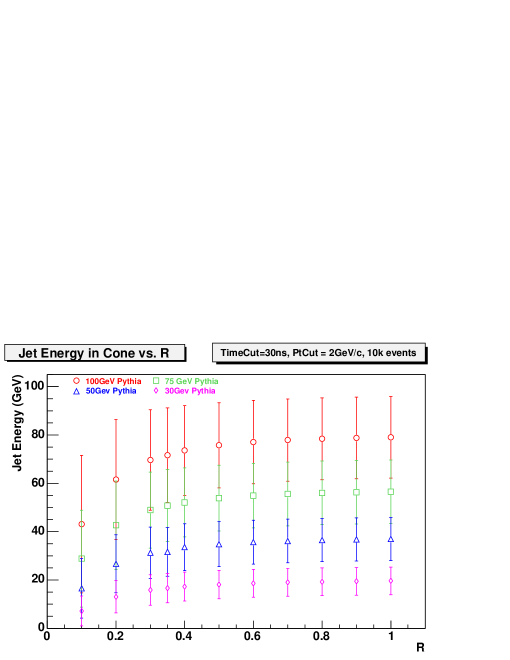
Fig. 3.8: Sum of $E_{T}$ for all tracks plus hits for pure PYTHIA jets of energies 100 GeV, 75 GeV, 50 GeV, 30 GeV respectively, within varying cone radii $R$.

Figs. 3.9-3.12 compare the amount of background energy and jet energy contained in the cone for varying $R$ (Note the different y-axis scales for the jet energy (left) and the background energy (right)). The symbols in the plots indicate the means and the error bars indicate the RMS of the distributions. For all jet energies presented, the mean background energy is greater than the jet energy in the cone for $R\geq 0.4$.

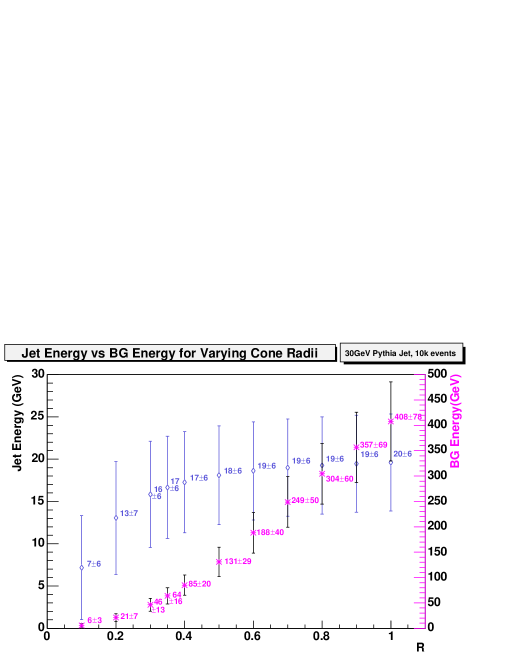
Fig. 3.9: Energy within varying cone radii, $R$, for 30 GeV jets compared to background energy. Symbols represent the mean of the distribution and error bars represent the RMS. The axis on the left is the jet energy scale and on the right is the background energy scale.

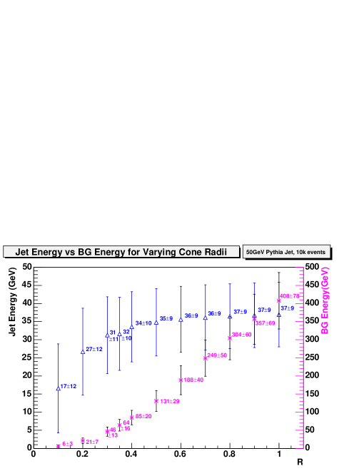
Fig. 3.10: As for Fig. 3.9 but jet energy = 50 GeV.

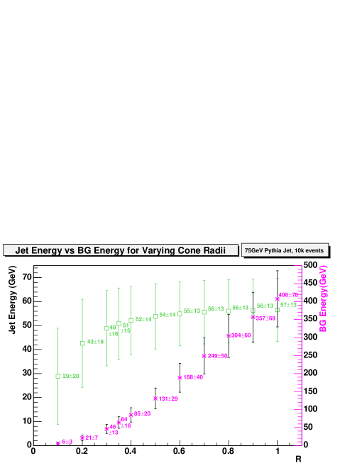
Fig. 3.11: As for Fig. 3.9 but jet energy = 75 GeV.

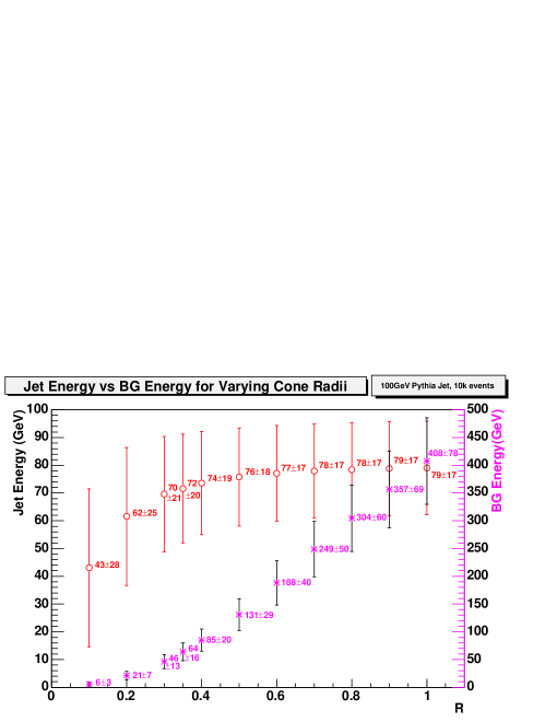
Fig. 3.12: As for Fig. 3.9 but jet energy = 100 GeV.

However, it is the size of the event-by-event fluctuations that provide the challenge to reconstructing the jet energies. In Fig. 3.13 the background fluctuation energies are plotted versus the jet energy in the cone for 50 GeV and 100 GeV jets. For 50 GeV jets for $R>0.5$, the event-by-event background energy fluctuations are larger than the jet energy in the cone making jet energy reconstruction impossible using $R>0.5$. This indicates that in order to find jets of lower energies ($E_{TJet}\sim$50 GeV), a relatively small cone size is required.

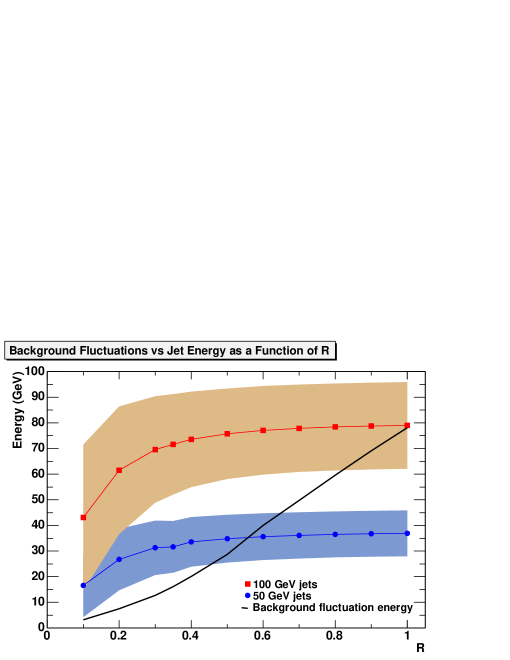
Fig. 3.13: Fluctuations in background energy within cone (solid line) compared to jet energy within cone for 50 GeV jets (circles) and 100 GeV jets (squares). The shaded area represents the RMS of the jet energy distributions.

Background Energy Fluctuations with Respect to Position on Grid

A further background energy study was performed to check that there was no significant bias in the grid energy deposit in terms of position on the grid. The detector setup in ALICE is not symmetrical and material in front of the EMCal could cause different particle absorption or scattering in certain directions. A ‘sliding patch’ method was used to calculate the size of the fluctuations by summing all the energy in the patch and plotting it divided by total grid energy as a function of patch position. The ‘patch’ was then slid to a new position such that the new patch position overlapped the old by half of the patch area. This process was repeated over the area of the grid. Fig. 3.14 shows that for a patch size equivalent to a cone radius of $R=0.1$, the fluctuations from place to place on the grid were of the order of $1\%$ and were due to statistical fluctuations.

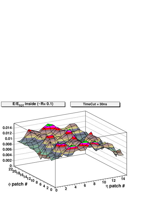
Fig. 3.14: Plots show energy contained in the patch, with equivalent area to $R=0.1$, divided by the total energy in the grid as a function of patch position.

3.2 Algorithm Optimisation

3.2.1 Parameter Optimisation

In order to optimise the reconstructed jet resolution and the jet finding efficiency, and to minimise the number of ‘fake’ jets reconstructed, the main algorithm parameters needed to be fine-tuned. These parameters are cone radius ($R$), minimum accepted jet seed tower energy ($JetESeed$) and the minimum accepted jet energy ($MinJetEt$). The parameters were optimised for the case of 50 GeV jets so that the majority of jets above this threshold would also be found and reconstructed. In order to reconstruct jets with $E_{T}<50$ GeV, alternative methods can be implemented, such as particle correlation methods which are currently used at experiments at RHIC [60] as discussed in Chapter 2.1.2.

Cone Radius ($R$)

From the study of background fluctuations in heavy-ion collisions, in Section 3.1.2, it was seen that for large cone radii, the absolute value of the background fluctuations is of the order of the jet energy contained in the cone. This implies that the use of smaller cone radii is preferable. On the other hand, very small cone radii ($R\leq 0.2$) contain around half of the total jet energy and this could lead to inaccuracies in reconstructing full jet energies. Thus various quantities, such as the amount of jet energy contained within different radii, and the resulting resolution of the reconstructed jet energy for different radii needed to be studied in order to find the optimal $R$ to be used in the cone algorithm for heavy-ion collisions.

Fig. 3.15 shows the percentage of jet energy contained within the cone as a function of cone radius $R$. The amount of jet energy contained inside the cone is found to saturate for $R\geq 0.6$. Note that even for $R=1.0$ the mean values are not expected to reach $100\%$ since energy due to neutrons is not measured and the $p_{T}$-cut also excludes some of the jet energy. It can also be seen that the $p_{T}$-cut has a larger effect on the lower energy jets since a larger fraction of particle energies from these jets are below the cut than is the case for the higher energy jets.

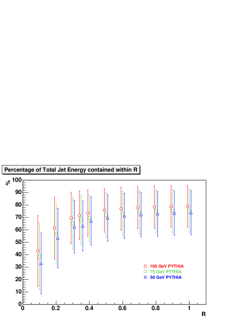
Fig. 3.15: Percentage of jet energy contained within different cone radii for 100 GeV (red circles), 75 GeV (green squares) and 50 GeV (blue triangles) jets. The symbols represent the mean and the error bars represent the RMS of the distributions. Symbols for 50 GeV and 100 GeV jets have been offset for clarity.

Another point to note, as can be seen in Fig. 3.16, is that the absolute value of the width of the jet energy distribution decreases as a function of $R$ (represented by the coloured triangles) which is the opposite behaviour to the background fluctuations (represented by the black circles). Therefore, in order to optimise the resolution of the reconstructed jets, the trade-off between the $R$-dependence of the background fluctuations and the jet energy widths needed to be analysed. The coloured stars in Fig. 3.16 represent the addition in quadrature of the RMS of the jet energy distributions and the background fluctuations.

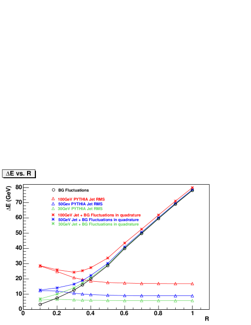
Fig. 3.16: $\Delta E$ as a function of cone radius $R$. The black circles represent the background fluctuations, the red/blue/green triangles represent the RMS of the 100GeV/50GeV/30GeV PYTHIA jet distributions and the coloured stars represent the sum in quadrature of the background fluctuations and the relevant jet energy widths.

Fig. 3.17 shows the resulting resolution, $\Delta E/E$, when the $\Delta E$ in Fig. 3.16 are divided by the pure PYTHIA jet energy contained in $R$. The stars represent what was classified as the ‘worst case’ scenario because the total value of the background fluctuations was added in quadrature to the jet energy widths when performing this calculation. When reconstructing the jet energy, the background energy was typically calculated and subtracted from the total energy in the jet cone and therefore using the total value of the background fluctuations is an overestimate of the contribution to the resolution from the background. However, it was important to find the upper limit on the jet energy resolution that was possible when using tracking plus calorimetry data. Fig. 3.17 also shows the ‘best case’ scenario for resolution (shown by the coloured triangles) which represents the $\Delta E/E$ of the pure PYTHIA distributions as a function of $R$. In this case, the energy from all detectable particles inside the cone of radius $R$ was summed around the known jet centre to find $\Delta E$ and $E$ (not jet finding results). This is therefore the limiting case on the best possible resolution using the cone method for the various detectors and the goal for which to aim when reconstructing jet energies.

As can also be seen from Fig. 3.17, the resolution for 30 GeV jets is very poor for almost all values of $R$ ($(\Delta E/E)_{30\rm{GeV}}>1$ for $R>0.3$) and thus optimisation was performed for the case of 50 GeV jets. For all values of $R$, the respective resolution for the case of 100 GeV jets is always better than that of 50 GeV jets. For 50 GeV jets the lowest value of $\Delta E/E=0.528$ when $R=0.3$. At $R=0.3$ the values of $\Delta E/E$ for the other jets are also close to their minimum values and therefore a cone radius of $R=0.3$ was chosen for jet reconstruction.

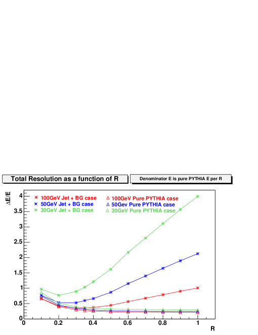
Fig. 3.17: $\Delta E/E$ as a function of $R$ where the $\Delta E$ are shown in Fig. 3.16 and where $E$ is the amount of pure PYTHIA energy contained in the respective $R$. The red/blue/green stars represent the 100 GeV/50 GeV/30 GeV PTYHIA plus background cases and the red/blue/green triangles represent the 100 GeV/50 GeV/30 GeV pure PYTHIA cases.

Jet Seed Energy ($JetESeed$) and Minimum Acceptable Jet Energy ($MinJetEt$)

In order to maximise the jet finding efficiency (fraction of input jets that are found and reconstructed) of the algorithm and minimise the number of ‘fake’ jets (jets found by the algorithm but that are not part of the input distribution) reconstructed, two further parameters needed to be tuned. The jet seed tower energy, $JetESeed$, and the minimum accepted jet energy, $MinJetEt$, were optimised by finding the best combination of the two parameters that give the optimal efficiency and minimal ‘fake’ jet rate. The $JetESeed$ and $MinJetEt$ act as two filters and are dependent on each other. If the $JetESeed$ is set low, in order not to exclude real jet seeds, this could allow a large number of ‘fake’ towers to be classified as jet seeds consequently requiring the $MinJetEt$ to be set with a high threshold to eliminate ‘fake’ jets while in turn preserving the real jets. It is also not optimal to set the $JetESeed$ too high because it was found to introduce a bias on the type of fragmentation process involved in forming the jet. i.e. this preselects processes which give rise to high-$p_{T}$ leading particles, biasing the resulting fragmentation function.

Note that ‘fake’ jets as classified above, are not always due to anomalous energy deposition (from fluctuations in the background which are then treated as jets by the algorithm), but can also be due to the presence of jets in the Central HIJING event. Although these are real jets, for the purpose of this analysis, all jets that were found that were not part of the input PYTHIA distribution were classified as ‘fakes’. For more detail on ‘fake’ jet classification in this thesis, refer to Chapter 4.3. Further study will need to be performed in order to separate and reconstruct multiple jets of different energies in the same event, but this is beyond the scope of this thesis.

Figs. 3.18 and 3.19 are graphical representations of the method used to find the optimal values for $JetESeed$ and $MinJetEt$. Fig. 3.18 shows the distribution of highest energy grid towers per event after background subtraction was performed for Central HIJING events alone (shown in blue) and for 50 GeV PYTHIA events combined with Central HIJING events (shown in green). The two distributions were found to overlap up to $\sim 20$ GeV although there was a 3 GeV difference in the means of the distributions with the PYTHIA events having a greater highest tower energy value than the pure HIJING events. The percentage of real jet seed exclusion and ‘fake’ jet seed inclusion for the first filter ($JetESeed$) could then be calculated for different values of $JetESeed$ by integrating the number of events that were above or below a chosen seed energy (an example of a 5 GeV seed energy is shown as the red line in Fig. 3.18).

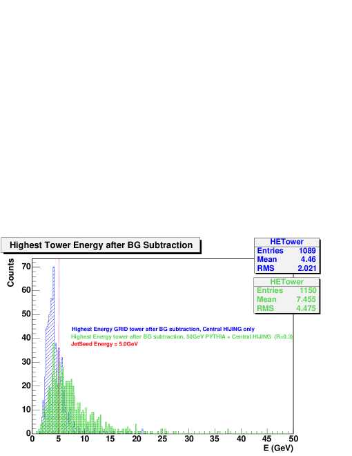
Fig. 3.18: Distribution of the energy of the highest energy tower per event after background subtraction, for Central HIJING events (in blue) and 50 GeV PYTHIA events combined with Central HIJING events (in green). The red line illustrates how a filter on seed tower energy would affect the inclusion/exclusion of background/jet events.

Since the two parameters depend on each other, the optimal value for $MinJetEt$ cannot be chosen from the first piece of analysis alone. Further analysis involved choosing a range of values of $JetESeed$ and, for each one, plotting the value of the energy, after background subtraction, inside a cone of radius $R=0.3$ for the case of Central HIJING events alone and for 50 GeV PYTHIA events combined with Central HIJING events. The situation for events passing a $JetESeed\geq 5$ GeV is shown in Fig. 3.19 where the pure Central HIJING events are shown in blue and the mixed events are shown in green. The real jet exclusion and ‘fake’ jet inclusion rates could then be calculated further for the case of different choices of $MinJetEt$ (per set value of $JetESeed$) by integrating the events above the relevant threshold (an example of $MinJetEt=10$ GeV is shown by the red line in the figure). Finally, the resulting inclusion and exclusion rates were tabulated as a function of the values of $JetESeed$ and $MinJetEt$. The optimal combination of parameters was chosen so as to produce the lowest inclusion rate of Central HIJING events while the inclusion rate of Parameterised HIJING 4000 events was less than $5\%$ and the exclusion of 50 GeV jets was less than $30\%$. The combination of parameters satisfying all these criteria can be found from Tables 3.1 - 3.4 and are $JetESeed=4.6$ GeV and $MinJetEt=14.0$ GeV.

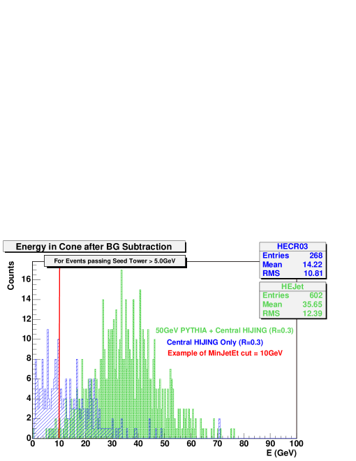
Fig. 3.19: Distribution of the energy inside a cone with $R=0.3$ after background subtraction for events that pass a filter of $JetESeed=5.0$ GeV. The case for Central HIJING events is shown in blue and the 50GeV PYTHIA combined with Central HIJING events is shown in green. The red line illustrates how a filter on minimum allowed jet $E_{T}$ would affect the inclusion/exclusion of background/jet events.

Parameter Values		50 GeV PYTHIA on Central HIJING
$JetESeed$ (GeV)	$MinJetEt$ (GeV)	Fraction passing $JetESeed$ ($\%$)	Fraction passing $MinJetEt$ ($\%$)	Fraction passing both filters ($\%$)	Fraction excluded ($\%$)
4.5	10.0	74.6	98.2	73.2	26.8
	10.5		97.8	72.9	27.1
	11.0		97.6	72.8	27.2
	12.0		97.3	72.6	27.4
	13.0		96.4	71.9	28.1
	14.0		95.1	70.9	29.1
4.6	10.0	73.2	98.5	72.1	27.9
	10.5		98.0	71.8	28.2
	11.0		97.7	71.6	28.4
	12.0		97.0	71.0	29.0
	13.0		96.5	70.7	29.3
	14.0		95.9	70.2	29.8
4.7	10.0	71.2	98.5	70.1	29.9
	10.5		98.5	70.1	29.9
	11.0		97.7	69.6	30.4
	12.0		97.2	69.2	30.8
	13.0		96.9	69.0	31.0
	14.0		95.7	68.1	31.9
4.8	10.0	70.3	98.1	69.0	31.0
	10.5		98.1	69.0	31.0
	11.0		97.8	68.8	31.2
	12.0		97.3	68.5	31.5
	13.0		96.9	68.1	31.9
	14.0		96.6	67.9	32.1
4.9	10.0	69.0	98.6	68.0	32.0
	10.5		98.2	67.8	32.2
	11.0		97.4	67.2	32.8
	12.0		96.6	66.7	33.3
	13.0		96.3	66.4	33.6
	14.0		95.7	66.0	34.0
5.0	10.0	67.3	98.5	66.3	33.7
	10.5		98.4	66.2	33.8
	11.0		98.2	66.1	33.9
	12.0		97.1	65.4	34.6
	13.0		96.8	65.1	34.9
	14.0		95.8	64.5	35.5
5.1	10.0	66.1	98.1	64.9	35.1
	10.5		98.0	64.8	35.2
	11.0		97.5	64.4	35.6
	12.0		96.6	63.9	36.1
	13.0		96.3	63.7	36.3
	14.0		95.4	63.1	36.9

Table 3.1: Exclusion rates for 50 GeV jets using various combinations of $JetESeed$ and $MinJetEt$.(Ratio background subtraction method was used.)

Parameter Values		100 GeV PYTHIA on Central HIJING
$JetESeed$ (GeV)	$MinJetEt$ (GeV)	Fraction passing $JetESeed$ ($\%$)	Fraction passing $MinJetEt$ ($\%$)	Fraction passing both filters ($\%$)	Fraction excluded ($\%$)
4.5	10.0	97.3	99.8	97.1	2.9
	10.5		99.8	97.1	2.9
	11.0		99.8	97.1	2.9
	12.0		99.8	97.1	2.9
	13.0		99.7	97.0	3.0
	14.0		99.5	96.8	3.2
4.6	10.0	96.8	99.9	96.7	3.3
	10.5		99.9	96.7	3.3
	11.0		99.9	96.7	3.3
	12.0		99.9	96.7	3.3
	13.0		99.8	96.6	3.4
	14.0		99.7	96.5	3.5
4.7	10.0	96.5	100.0	96.5	3.5
	10.5		99.9	96.4	3.6
	11.0		99.8	96.3	3.7
	12.0		99.7	96.2	3.8
	13.0		99.6	96.1	3.9
	14.0		99.6	96.1	3.9
4.8	10.0	96.4	99.9	96.3	3.7
	10.5		99.9	96.3	3.7
	11.0		99.9	96.3	3.7
	12.0		99.8	96.2	3.8
	13.0		99.8	96.2	3.8
	14.0		99.8	96.2	3.8
4.9	10.0	96.0	99.8	95.8	4.2
	10.5		99.8	95.8	4.2
	11.0		99.7	95.7	4.3
	12.0		99.7	95.7	4.3
	13.0		99.7	95.7	4.3
	14.0		99.7	95.7	4.3
5.0	10.0	95.8	99.8	95.6	4.4
	10.5		99.8	95.6	4.4
	11.0		99.8	95.6	4.4
	12.0		99.8	95.6	4.4
	13.0		99.8	95.6	4.4
	14.0		99.6	95.4	4.6
5.1	10.0	95.3	100.0	95.3	4.7
	10.5		100.0	95.3	4.7
	11.0		100.0	95.3	4.7
	12.0		100.0	95.3	4.7
	13.0		99.9	95.2	4.8
	14.0		99.9	95.2	4.8

Table 3.2: Exclusion rates for 100 GeV jets using various combinations of $JetESeed$ and $MinJetEt$.

Parameter Values		Pure Central HIJING
$JetESeed$ (GeV)	$MinJetEt$ (GeV)	Fraction passing $JetESeed$ ($\%$)	Fraction passing $MinJetEt$ ($\%$)	Fraction passing both filters ($\%$)
4.5	10.0	36.9	49.3	18.2
	10.5		48.2	17.8
	11.0		46.8	17.3
	12.0		43.9	16.2
	13.0		40.6	15.0
	14.0		38.0	14.0
4.6	10.0	34.1	49.7	16.9
	10.5		48.5	16.5
	11.0		47.0	16.0
	12.0		44.8	15.3
	13.0		41.2	14.0
	14.0		38.7	13.2
4.7	10.0	32.6	49.7	16.2
	10.5		48.4	15.8
	11.0		46.8	15.3
	12.0		44.6	14.6
	13.0		40.8	13.3
	14.0		38.5	12.6
4.8	10.0	30.0	50.2	15.1
	10.5		48.8	14.7
	11.0		47.1	14.1
	12.0		44.6	13.4
	13.0		41.5	12.5
	14.0		39.4	11.9
4.9	10.0	28.7	49.8	14.3
	10.5		48.3	13.8
	11.0		47.1	13.5
	12.0		44.8	12.8
	13.0		41.7	12.0
	14.0		39.8	11.4
5.0	10.0	27.9	49.6	13.8
	10.5		48.1	13.4
	11.0		46.3	12.9
	12.0		44.0	12.3
	13.0		40.7	11.3
	14.0		38.4	10.7
5.1	10.0	25.2	49.2	12.4
	10.5		47.9	12.1
	11.0		46.3	11.6
	12.0		43.8	11.0
	13.0		40.1	10.1
	14.0		37.6	9.5

Table 3.3: Inclusion rates for pure Central HIJING events using various combinations of $JetESeed$ and $MinJetEt$.

Parameter Values		Parameterised HIJING 4000
$JetESeed$ (GeV)	$MinJetEt$ (GeV)	Fraction passing $JetESeed$ ($\%$)	Fraction passing $MinJetEt$ ($\%$)	Fraction passing both filters ($\%$)
4.5	10.0	18.5	31.2	5.8
	10.5		27.7	5.1
	11.0		26.6	4.9
	12.0		24.9	4.6
	13.0		19.7	3.6
	14.0		15.6	2.9
4.6	10.0	16.6	30.3	5.0
	10.5		27.1	4.5
	11.0		25.8	4.3
	12.0		23.9	4.0
	13.0		19.4	3.2
	14.0		15.5	2.6
4.7	10.0	14.0	32.1	4.5
	10.5		28.2	4.0
	11.0		27.5	3.8
	12.0		25.2	3.5
	13.0		19.8	2.8
	14.0		16.0	2.2
4.8	10.0	12.4	32.8	4.1
	10.5		28.4	3.5
	11.0		27.6	3.4
	12.0		25.9	3.2
	13.0		19.8	2.5
	14.0		15.5	1.9
4.9	10.0	11.3	33.0	3.7
	10.5		29.2	3.3
	11.0		28.3	3.2
	12.0		26.4	3.0
	13.0		19.8	2.2
	14.0		15.1	1.7
5.0	10.0	10.4	34.0	3.5
	10.5		29.9	3.1
	11.0		28.9	3.0
	12.0		26.8	2.8
	13.0		20.6	2.1
	14.0		15.5	1.6
5.1	10.0	9.7	35.2	3.4
	10.5		30.8	3.0
	11.0		29.7	2.9
	12.0		27.5	2.7
	13.0		22.0	2.1
	14.0		16.5	1.6

Table 3.4: Inclusion rates for parameterised HIJING 4000 events using various combinations of $JetESeed$ and $MinJetEt$.

The case for a seedless algorithm ($JetESeed=0$ GeV) was studied in the same way and the resulting inclusion and exclusion rates can be seen in Table 3.5. In order to compare jet finding results for the two cases of a seedless algorithm and seeded algorithm, a value of $MinJetEt$ was chosen such that the inclusion rate of Central HIJING events was approximately the same ($\sim$13$\%$) as for the case of the seeded algorithm where $JetESeed=4.6$ GeV and $MinJetEt=14.0$ GeV. The value for the seedless case which fulfilled this criterion was $MinJetEt=20.0$ GeV.

Parameter Value	50 GeV PYTHIA on Central HIJING	100 GeV PYTHIA on Central HIJING	Central HIJING	Param. HIJING 4000
$MinJetEt$ (GeV)	Exclusion rate ($\%$)	Exclusion rate ($\%$)	Inclusion rate ($\%$)	Inclusion rate ($\%$)
10.0	6.2	0.9	37.7	21.8
10.5	6.7	1.0	36.0	19.3
11.0	7.1	1.2	34.1	18.1
11.5	7.7	1.3	32.2	16.9
12.0	8.1	1.3	30.0	15.4
12.5	8.7	1.4	28.9	14.5
13.0	9.1	1.5	27.1	13.2
13.5	9.2	1.5	25.6	12.1
14.0	9.9	1.6	23.9	11.1
14.5	10.6	1.6	23.3	10.3
15.0	11.6	1.6	22.2	9.3
15.5	12.3	1.7	20.8	8.7
16.0	12.9	1.7	19.6	8.1
16.5	13.6	1.7	18.5	7.5
17.0	13.9	1.7	17.8	6.7
17.5	14.5	1.8	17.3	5.9
18.0	15.5	2.0	16.7	4.9
18.5	16.2	2.0	16.1	4.5
19.0	17.1	2.0	15.0	4.0
19.5	18.2	2.1	13.8	3.7
20.0	19.1	2.2	13.1	3.0
20.5	20.1	2.3	12.4	2.9
21.0	20.9	2.3	11.4	2.5
21.5	22.0	2.4	10.4	2.1
22.0	22.8	2.7	10.1	1.8
22.5	23.6	2.7	9.6	1.7
23.0	25.0	3.0	9.0	1.3
23.5	26.8	3.2	8.0	1.3
24.0	28.1	3.4	7.6	1.3
24.5	29.0	3.5	7.2	1.1
25.0	30.5	3.6	6.4	0.9

Table 3.5: Exclusion and inclusion rates for the case of a seedless algorithm ($JetESeed=0$ GeV).

3.2.2 Methods Optimisation

Calculation of the Background Energy in the Jet Cone

Accurate calculation of the background energy contribution inside the jet cone was necessary to enable accurate reconstruction of the energies of the jets found by the jet finding algorithm. A number of approaches, including statistical, event-by-event and a combination of both were attempted in order to calculate most accurately the background energy inside the jet cone.

• Statistical Method
  The Statistical Method calculates the background energy contribution inside the jet cone on an average basis by summing the energy in the grid from 1 000 Central HIJING events and finding the mean energy per event. This energy can then be scaled to the size of the cone radius used in jet finding and subtracted for each event on which jet finding is performed. However, when this calculated background energy is compared to the actual summed background energy event-by-event, it is found that the width of the distribution of the difference in the two quantities is large. This is due to the effect of event-by-event energy fluctuations. The average difference in the quantities is close to zero as shown in Fig. 3.21 (black symbols) but the RMS is larger (represented by the error bars) than is the case for event-by-event calculation methods.

The event-by-event methods were developed to take into account the fact that the event-by-event background fluctuations are large. The methods are based on the assumption that the distribution of the background energy in the grid is uniform, as was shown in Section 3.1.2.

• Cone Method
  The Cone Method calculates the background contribution to the energy inside the jet cone as follows: once the jet cone is found by the jet finding algorithm, all the energy in the grid outside the jet cone is summed and then scaled for the size of the cone radius. This amount is then subtracted from the energy inside the jet cone to calculate the actual jet energy. This calculation is performed on an event-by-event basis (in fact, sometimes more than once per event depending on the number of iterations performed by the algorithm). The accuracy of the Cone Method background calculation also depends on the size of the cone radius used since the bigger the cone radius, the less area there is outside the cone on which to base the background calculation, see Fig. 3.21.

In addition to event-by-event background energy fluctuations, there are also statistical fluctuations in the background energy deposited in the grid from tower to tower. Further fluctuations on a tower level, caused by implementing the track $p_{T}$-cut, are also present.

• Ratio Method
  A second event-by-event method, Ratio Method, was developed to further reduce the effect of the fluctuations. The method is based on the Cone Method calculation but with some differences: firstly, two grids are used to store the energy information. The first grid is the same as the grid used in the Cone Method and is composed of the energy from the hits in the EMCal plus the energy from all the tracks which pass the $p_{T}$-cut. The second grid however, is composed of the energy from hits and all the track energy without a $p_{T}$-cut implemented. Jet finding is performed on the first grid but once the jet cone is found by the algorithm, the energy outside the cone in the second grid is summed and scaled for the cone radius, $E_{Cone_{NoCuts}}$. Next, the actual background energy contribution, $E_{Cone_{Cuts}}$, to be subtracted from the jet cone energy in the first grid is calculated by multiplying $E_{Cone_{NoCuts}}$ by the ratio $F=E_{BG_{Cuts}}/E_{BG_{NoCuts}}$. The ratio, $F$, was found by calculating the average, over 1000 Central HIJING events, of the energy in the grid with a $p_{T}$-cut divided by the energy in the grid without a $p_{T}$-cut as shown in Fig. 3.20.

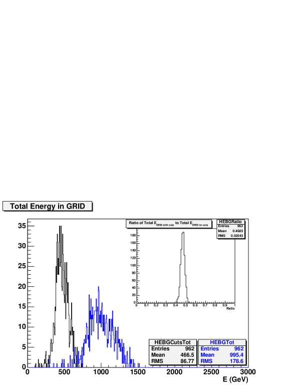
Fig. 3.20: Distribution of total energy contained in the grid from Central HIJING events. The blue histogram shows the energy in the grid from events without a $p_{T}$-cut and the black histogram shows the case with a $p_{T}$-cut $=2$ GeV. The inset shows the ratio $E_{cuts}/E_{NoCuts}=0.4685$ of the two histograms.

A comparison of the 3 background energy calculation methods can be seen in Fig. 3.21. This shows the difference between the calculated values and the actual amount of background energy that was summed in the cone as a function of cone radius $R$. All three methods resulted in means that lay close to the true value of the background energy for all $R$ but the error (shown by error bars) was smallest for the Ratio Method. Therefore the Ratio Method was chosen as the preferred background calculation method to be used in the jet finding algorithm.

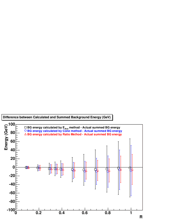
Fig. 3.21: Difference between background energy calculated using Statistical($E_{Ave}$) /$Cone$/$Ratio$ methods and the actual summed background energy inside varying cone radii shown by black/blue/red symbols. The error bars represent the RMS of the respective distributions. Symbols for Statistical$(E_{Ave})$ and $Ratio$ methods have been offset for clarity.

Chapter 4 Results with the Optimised ALICE Algorithm

This chapter is divided into four main sections, Reconstruction Accuracy, Jet Energy Correction, Reconstruction Efficiency, and Energy Resolution. The section discussing energy resolution is placed last in order to be able to compare the resolutions for different cases discussed in the previous sections.

4.1 Reconstruction Accuracy

The jet reconstruction results using the ALICE jet finding algorithm in both its seeded and seedless versions are presented. The values of the parameters used in both cases are shown in Table 4.1. The TPC efficiency quoted in the table is not a parameter but is a conservative estimate of the TPC tracking efficiency which was set in the analysis. For the case of the seeded algorithm, for comparison, jet finding is performed on a combination of tracking and calorimeter data and additionally, on tracking data alone. For the seedless algorithm case, jet finding is performed on a combination of tracking and calorimetry data.

Algorithm	$R$	$JetESeed$ (GeV)	$MinJetEt$ (GeV)	BG Method	TPC efficiency
Seeded	0.3	4.6	14.0	Ratio	$90\%$
Seedless	0.3	0.0	20.0	Ratio	$90\%$

Table 4.1: Optimised parameters for the seeded and seedless versions of the algorithm.

4.1.1 Seeded Algorithm Results

Results for tracking plus calorimetry data

The reconstructed energy distributions for 50 GeV, 75 GeV and 100 GeV PYTHIA jets on Central HIJING background (i.e. combined events) are shown in Figs. 4.1-4.3. As expected, the reconstructed jet energies, in all cases, are lower than the input jet energies. This is due to the cone radius of $R=0.3$ putting a constraint on the amount of jet energy contained within the cone, the energy from neutral hadrons being excluded as it was not measured and the $p_{T}$-cut on track energies. The sharp cut-off in the jet energy distributions at 14 GeV is due to the $MinJetEt$ parameter setting.

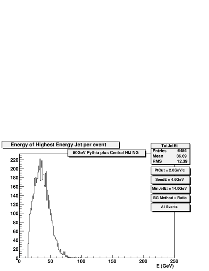
Fig. 4.1: Reconstructed jet energy distribution for input 50 GeV PYTHIA jets on Central HIJING background.

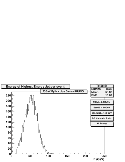
Fig. 4.2: Reconstructed jet energy distribution for input 75 GeV PYTHIA jets on Central HIJING background.

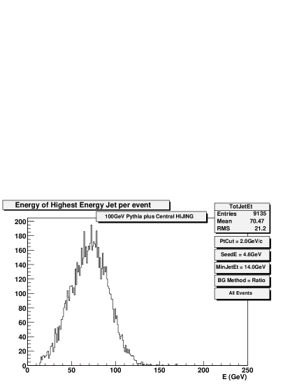
Fig. 4.3: Reconstructed jet energy distribution for input 100 GeV PYTHIA jets on Central HIJING background.

For comparison, the algorithm was also applied to pure PYTHIA events with no added background with identical parameters (except for background subtraction which used the Cone Method). Table 4.2 shows, for both the combined and pure PYTHIA events, the resulting mean jet energies as a percentage of the input nominal jet energies. Thus the algorithm produces results for the combined events which are within $10\%$ of the results for pure PYTHIA events.

Corrections to the reconstructed jet energy can be made to account for the losses due to the $p_{T}$-cut and small cone radius by using a cross-section weighted multiplicative factor as discussed in section 4.2. When the experiment goes live, $\gamma$-jet events will be used to calibrate the reconstructed jet energies, see section 4.2. A detailed description of jet energy calibration will not be discussed in detail in this thesis.

Event Type	$\langle E_{Reco}\rangle/E_{Input}$ for 50 GeV input jet	$\langle E_{Reco}\rangle/E_{Input}$ for 75 GeV input jet	$\langle E_{Reco}\rangle/E_{Input}$ for 100 GeV input jet
Combined	0.73	0.71	0.70
Pure PYTHIA	0.64	0.65	0.66

Table 4.2: $\langle E_{Reco}\rangle/E_{Input}$ for combined events and pure PYTHIA events for the cases of 50 GeV, 75 GeV and 100 GeV input jets.

In order to measure the accuracy of the reconstructed jet directions as calculated by the algorithm, the difference between the reconstructed jet direction, in ($\eta,\phi$)-space, and the original parton direction, from the PYTHIA event, was calculated for each combined event on which jet finding was performed. Histograms showing $\Delta\eta=\eta^{Reco}_{Jet}-\eta^{Input}_{Jet}$ and $\Delta\phi=\phi^{Reco}_{Jet}-\phi^{Input}_{Jet}$ for the range of input jet energies are shown in Figs. 4.4-4.6. The maxima of the histograms are peaked at zero, for all cases, showing that on average the correct jet direction is found. The accuracy of the direction reconstruction increases with increasing input jet energy as can be seen by comparing the RMS values which are plotted in Fig. 4.7. Also shown in Fig. 4.7 are the RMS results for the algorithm applied to pure PYTHIA events. The RMS values for the combined events are larger than for the pure PYTHIA events, but approach the same value as the input jet energy increases.

Fig. 4.4: Difference between reconstructed jet directions and the input jet direction for 50 GeV PYTHIA events on Central HIJING background.

Fig. 4.5: Difference between reconstructed jet directions and the input jet direction for 75 GeV PYTHIA events on Central HIJING background.

Fig. 4.6: Difference between reconstructed jet directions and the input jet direction for 100 GeV PYTHIA events on Central HIJING background.

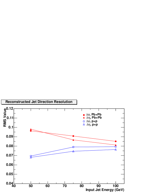
Fig. 4.7: RMS of reconstructed jet $\Delta\eta$ and $\Delta\phi$ distributions for the combined events (Pb+Pb) (closed symbols) case compared to the pure PYTHIA (p+p) case (open symbols).

Results for tracking data alone

In order to understand the accuracy and efficiency of the jet finding algorithm in the case that only tracking information is available, jet finding was performed on charged tracking data only, for PYTHIA events combined with Central HIJING events. The reconstructed energy distributions can be seen in Figs. 4.8-4.10.

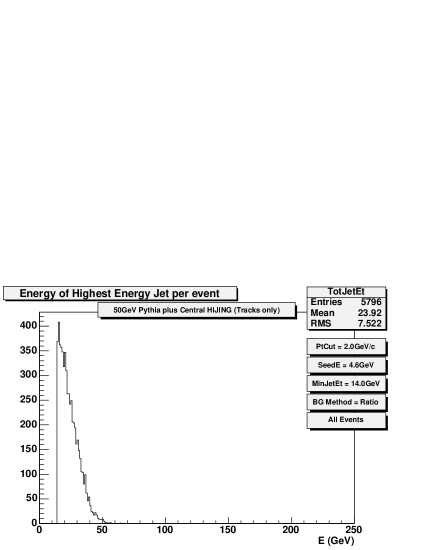
Fig. 4.8: Reconstructed jet energy distribution for input 50 GeV PYTHIA jets on Central HIJING background using tracking data alone.

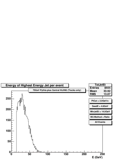
Fig. 4.9: Reconstructed jet energy distribution for input 75 GeV PYTHIA jets on Central HIJING background using tracking data alone.

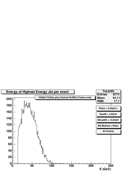
Fig. 4.10: Reconstructed jet energy distribution for input 100 GeV PYTHIA jets on Central HIJING background using tracking data alone.

Compared to the reconstructed jet energy distributions from the tracking plus calorimetry data, the distributions for tracking data alone have a larger shift towards lower reconstructed jet energies. Table 4.3 shows the percentage of total nominal jet energy reconstructed using tracking data alone compared to tracking plus calorimetry data. There is $\sim$25$\%$ less jet energy reconstructed when using tracking data alone compared to when using a combination of tracking plus calorimetry data. However, it is still possible to reconstruct jets using the jet finding algorithm with the seeded parameters on tracking data alone although the resulting energy resolutions are worse than when a combination of tracking and calorimetry data is used, see Section 4.4.

Data Type	$\langle E_{Reco}\rangle/E_{Input}$ for 50 GeV input jet	$\langle E_{Reco}\rangle/E_{Input}$ for 75 GeV input jet	$\langle E_{Reco}\rangle/E_{Input}$ for 100 GeV input jet
Tracking plus calorimetry	0.73	0.71	0.70
Tracking alone	0.48	0.45	0.44

Table 4.3: $\langle E_{Reco}\rangle/E_{Input}$ for the seeded algorithm case using tracking plus calorimetry data vs. tracking data alone. Both sets of events used were combined events.

The accuracy with which the algorithm can reconstruct jet directions using only tracking data can be seen in Figs. 4.11-4.13. The maxima of the histograms are peaked at zero as was the case for the tracking plus calorimetry results but the widths of the $\Delta\eta$ distributions are $\sim$12$\%$ greater than in the tracks plus calorimetry case. The $\Delta\phi$ distributions are up to $9\%$ greater as shown in Table 4.4. Therefore, direction reconstruction accuracy decreases when only tracking information is used to reconstruct jets. A comparison between the results using tracking plus calorimetry information and tracking information only, is shown in Fig. 4.14.

Fig. 4.11: Difference between reconstructed jet directions and the input jet direction for 50 GeV PYTHIA events on Central HIJING background using tracking data alone.

Fig. 4.12: Difference between reconstructed jet directions and the input jet direction for 75 GeV PYTHIA events on Central HIJING background using tracking data alone.

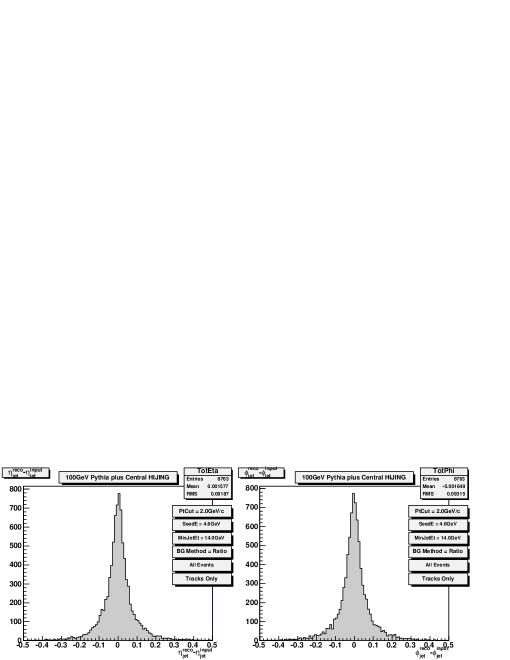
Fig. 4.13: Difference between reconstructed jet directions and the input jet direction for 100 GeV PYTHIA events on Central HIJING background using tracking data alone.

Data Type	RMS Value for 50GeV distribution		RMS Value for 75GeV distribution		RMS Value for 100GeV distribution
	$\Delta\eta$ RMS	$\Delta\phi$ RMS	$\Delta\eta$ RMS	$\Delta\phi$ RMS	$\Delta\eta$ RMS	$\Delta\phi$ RMS
Tracking plus calorimetry	0.098	0.096	0.087	0.091	0.081	0.085
Tracking alone	0.110	0.104	0.096	0.093	0.092	0.093

Table 4.4: Comparison of the RMS values for the $\Delta\eta$ and $\Delta\phi$ distributions for jet finding results from tracking plus calorimetry data and tracking data alone.

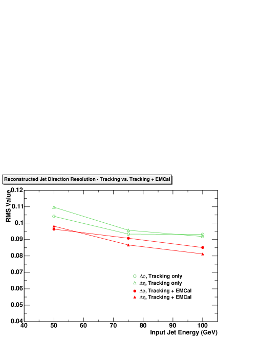
Fig. 4.14: RMS of the reconstructed jet $\Delta\eta$ and $\Delta\phi$ distributions for combined events with tracking and calorimetry information (solid symbols) compared to events using only tracking information (open symbols).

4.1.2 Seedless Algorithm Results

Results for tracking plus calorimetry data

Figs. 4.15-4.17 show the reconstructed jet energy distributions for the case of zero seed energy. The reconstructed mean energies are slightly lower than those for the seeded algorithm case, see Table 4.5. However, the shape of the seedless distributions is skewed to lower energies compared to the seeded case. This is due to a higher number of ‘fake’ jets being included by the algorithm as real jets in the distribution, (discussed in Section 4.3), when the seed energy is set to zero. The sharp cut-off in the jet energy distributions at 20 GeV is due to the MinJetEt parameter setting.

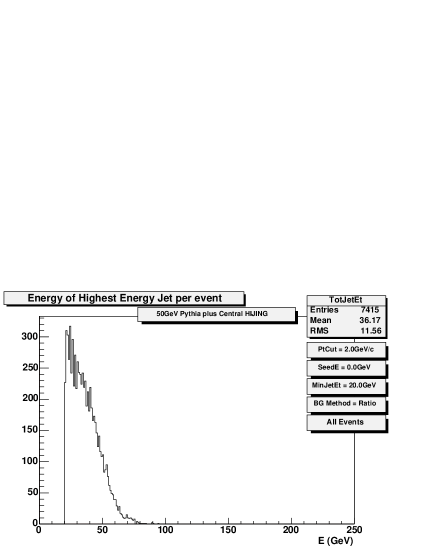
Fig. 4.15: Reconstructed jet energy distribution for input 50 GeV PYTHIA jets on Central HIJING background using the seedless algorithm.

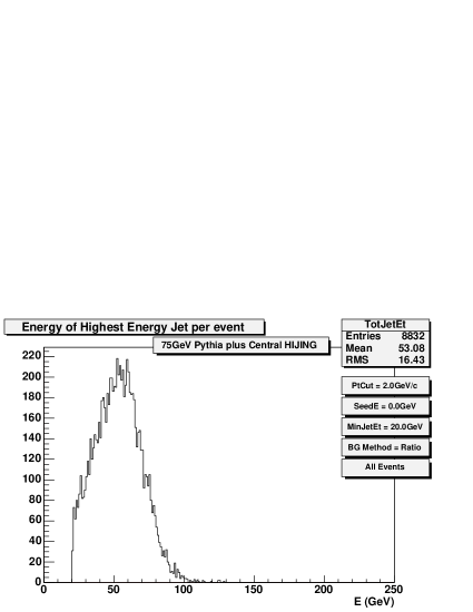
Fig. 4.16: Reconstructed jet energy distribution for input 75 GeV PYTHIA jets on Central HIJING background using the seedless algorithm.

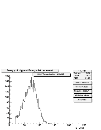
Fig. 4.17: Reconstructed jet energy distribution for input 100 GeV PYTHIA jets on Central HIJING background using the seedless algorithm.

Algorithm Type	$\langle E_{Reco}\rangle$ for 50GeV input jet (GeV)	$\langle E_{Reco}\rangle$ for 75GeV input jet (GeV)	$\langle E_{Reco}\rangle$ for 100GeV input jet (GeV)
Seeded	36.69	53.06	70.47
Seedless	36.17	53.08	70.32

Table 4.5: Reconstructed mean jet energies for various input jet energies for the case of the seeded algorithm vs. the seedless algorithm.

The difference between the reconstructed jet directions and the input directions are shown in Figs. 4.18-4.20. The widths of the $\Delta\eta$ and $\Delta\phi$ distributions are $\sim$30$\%$ greater in the seedless case compared to the seeded case for 50 GeV input jets. However, the difference between the two cases decreases with increasing input jet energy and for 100 GeV input jets, the spread is $\sim$3$\%$ greater for the seedless case than the seeded case. Table 4.6 shows the widths of the reconstructed jet directions for the seedless case compared to the seeded case. The top line of the table is taken from Table 4.4. Therefore, from Table 4.6, it can be seen that the seeded algorithm reconstructs jet directions more accurately than the seedless algorithm.

Algorithm Type	RMS Value for 50GeV distribution		RMS Value for 75GeV distribution		RMS Value for 100GeV distribution
	$\Delta\eta$ RMS	$\Delta\phi$ RMS	$\Delta\eta$ RMS	$\Delta\phi$ RMS	$\Delta\eta$ RMS	$\Delta\phi$ RMS
Seeded	0.098	0.096	0.087	0.091	0.081	0.085
Seedless	0.129	0.122	0.095	0.097	0.085	0.087

Table 4.6: Comparison of the RMS values for the $\Delta\eta$ and $\Delta\phi$ distributions for jet finding results from the seeded algorithm vs. the seedless algorithm for tracking plus calorimetry data.

Fig. 4.18: Difference between reconstructed jet directions and the input jet direction for 50 GeV PYTHIA events on Central HIJING background using the seedless algorithm.

Fig. 4.19: Difference between reconstructed jet directions and the input jet direction for 75 GeV PYTHIA events on Central HIJING background using the seedless algorithm.

Fig. 4.20: Difference between reconstructed jet directions and the input jet direction for 100 GeV PYTHIA events on Central HIJING background using the seedless algorithm.

4.2 Jet Energy Correction

When the first ALICE data is available, jet energies will be calibrated experimentally by measuring the $\gamma$-jet process. The energy of the observed photon will be the same as the energy of the jet, due to energy conservation, and therefore its energy can be used to calibrate the measured jet energy.

Presented here is a simple correction which may be applied to jet results in the absence of the calibration to real data. This correction takes all detector and algorithm effects on the jet energy into account simultaneously and involves the multiplication of the reconstructed jet energy by a constant factor $C$.

The jet energies reconstructed by the optimised algorithms are shifted to lower energies as shown by the reconstructed jet energy distribution plots in section 4.1. There are four main contributions to the energy shift. Using a small cone radius ($R=0.3$) in the jet finding algorithm leads to the exclusion of energy from jet particles which are outside the cone but which are really part of the jet. Performing a $p_{T}$-cut of 2 GeV/$c$ on all charged tracks further excludes some jet energy. Energy is also excluded from jet particles which are not measurable in the detectors (e.g. $K_{L}$). The final contribution is due to the event-by-event energy fluctuations in the underlying event which cause a small shift to higher energy from inaccuracies in the background energy calculation, see Table 4.7. However this shift is smaller than the combined shift of the other three contributions in the opposite direction. This is shown by comparing the fraction of jet energy contained within a cone of radius $R=0.3$ for pure PYTHIA events and combined events. The fraction is lower for pure PYTHIA events with no background than for combined events (see Table 4.7). The fractions are obtained by fitting the reconstructed jet energy distributions to a gaussian distribution and taking the mean from the fit divided by the input jet energy.

	50 GeV Input	75 GeV Input	100 GeV Input
$\langle E_{Reco}\rangle$ / $E_{Input}$ (pure PYTHIA)	64.08 $\%$	64.89 $\%$	65.90 $\%$
$\langle E_{Reco}\rangle$ / $E_{Input}$ (combined events)	67.08 $\%$	68.83 $\%$	69.33 $\%$

Table 4.7: Percentage jet energy contained within $R=0.3$ for pure PYTHIA events and combined events using the seeded algorithm.

As shown in Table. 4.7, the percentage of total jet energy contained inside $R=0.3$ increases as a function of jet energy for pure PYTHIA events and combined events. However, when jets are reconstructed in experiment, it is not known a priori what the real jet energy was. Therefore the factor $C$, by which jet energies are to be multiplied, needs to be independent of jet energy.

In this case, $C$ was calculated for the case of combined events (Pb+Pb case), by weighting the fraction of jet energy contained inside $R=0.3$ by the appropriate cross-section for 50 GeV, 75 GeV and 100 GeV jet production. The resulting value is: $C=1/0.6731$.

The resulting jet energy distributions for 50 GeV, 75 GeV and 100 GeV jets before and after performing the energy correction, are shown in Figs. 4.21-4.23. (In this case, a different sample of data was used compared to other analysis in this chapter for technical programming reasons. However the two sets of data are consistent.) The means and $\sigma$ of the fitted shifted distributions are shown in Table. 4.8. The corrected means are within $4\%$ of the input jet energies for the three samples. Therefore it is possible to use one multiplicative factor, $C$, to perform a successful jet energy correction over a range of jet energies.

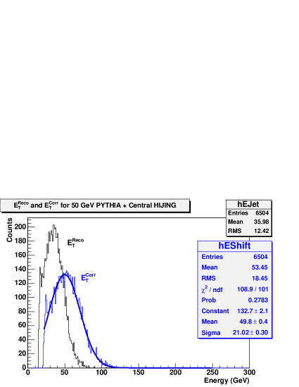
Fig. 4.21: Reconstructed ($E_{T}^{Reco}$) and corrected ($E_{T}^{Corr}$) jet energy distributions for 50 GeV jets using the method described in the text.

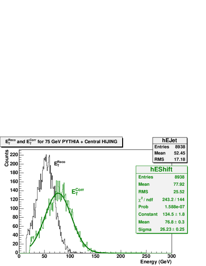
Fig. 4.22: Reconstructed ($E_{T}^{Reco}$) and corrected ($E_{T}^{Corr}$) jet energy distributions for 75 GeV jets using the method described in the text.

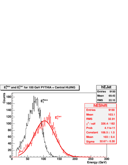
Fig. 4.23: Reconstructed ($E_{T}^{Reco}$) and corrected ($E_{T}^{Corr}$) jet energy distributions for 100 GeV jets using the method described in the text.

	50 GeV Input	75 GeV Input	100 GeV Input
$\langle E_{Corr}\rangle$ (combined events) (GeV)	49.8	76.8	103.0
$\sigma$ (combined events) (GeV)	21.0	26.2	32.7

Table 4.8: Corrected mean energies and $\sigma$ after fitting shifted energy distributions with a gaussian distribution.

4.3 Reconstruction Efficiency

4.3.1 Efficiency and ‘Fake’ Rates

The jet reconstruction efficiency, $\epsilon$, of the algorithm can be defined as the number of reconstructed jets divided by the number of known input jets:

$$\epsilon=\frac{N^{Reco}_{Jets}}{N^{Input}_{Jets}}$$ (4.1)

for a given sample of events. If $\epsilon=1$, it implies that all the input jets were found and reconstructed. It is therefore the aim when optimising the algorithm to ensure that $\epsilon$ is as close to 1 as possible. If $\epsilon>1$ then the jet finding algorithm found more jets than were input.

The case of $\epsilon>1$ could happen for a number of reasons:

• ‘Underlying Event’ Fluctuations
  In the high multiplicity background environment of Central HIJING events, with large event-by-event fluctuations and mini-jets present, it is possible that the algorithm could mistake a large random fluctuation or mini-jet for a jet. PYTHIA events contain an ‘underlying event’ which may lead to fluctuations in the measured energy deposition in the detectors that the algorithm could mistake for a real jet. These reconstructed jets will be classified as ‘fake’ jets.

• Unknown ‘Real’ Jets
  There is a significant cross-section for jet production in Central HIJING events at LHC energies, and therefore, there is the possibility that some of these jets fall within the EMCal fiducial volume and are reconstructed by the algorithm. There is also the possibility that the PYTHIA jet event contains more than two jets in it since the simulation condition was that at least one jet must point in the direction of the EMCal (trigger jet) while no constraint was put on the maximum number of jets in the event. These extra jets could fall within the EMCal fiducial volume and be reconstructed by the algorithm. In this case, although the reconstructed jets are real, since there is no prior information about them as they are not purposely triggered on, they are treated as ‘fake’ jets in this thesis to differentiate them from the known PYTHIA input jets. Fig. 4.24 shows an event that is likely to be of this type.

  

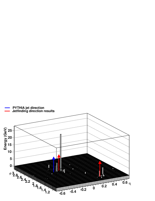
  Fig. 4.24: Grid energy including tracking and calorimetry information for a PYTHIA event with a 100 GeV jet where the algorithm reconstructed two jets. The blue arrow indicates the direction of the trigger jet as calculated by PYTHIA and the red arrows indicate the directions of the two jets reconstructed by the algorithm.

  The figure shows the energy grid containing track and calorimetry information for a PYTHIA event, containing a 100 GeV jet, in which the seeded algorithm reconstructed two jets. The direction of the trigger jet as calculated by PYTHIA is indicated by the blue arrow ($\eta$=-0.29, $\phi$=2.22) and the directions of the two jets reconstructed by the algorithm are shown by the red arrows ($\eta_{1}$=-0.20, $\phi_{1}$=2.22) and ($\eta_{2}$=0.24, $\phi_{2}$=1.32). The jets reconstructed by the algorithm have cone centres with an angular distance of $D=\sqrt{{(\Delta\eta)}^{2}+{(\Delta\phi)}^{2}}=1.00$ away from each other. Therefore they are out of range of each other’s centres to be included within a cone radius of up to $R=1.0$, the typical cone jet definition. The angular distance of the trigger jet cone centre, as calculated by PYTHIA, from the centre of mass of the other energy deposit ($\eta_{2}$, $\phi_{2}$) is $R=1.04$. Therefore, the energy deposits reconstructed as two jets by the algorithm, are most likely real separate jets although the lower energy jet would be counted as a ‘fake’ jet in this thesis. The proportion of PYTHIA events which contained two or more reconstructed jets and which satisfied the following condition:

  1. (2R) $D>1.0$, where $D$ is the angular distance between the two reconstructed jets,

  are shown in Table.4.9.

  	50 GeV Sample	75 GeV Sample	100 GeV Sample
  Percentage of events with $>1$ recon. jet and satisfying condition 1(2R)	0.02$\%$	0.08$\%$	0.17$\%$

  Table 4.9: Contribution to ‘fake’ rate from events containing at least 2 real PYTHIA jets within the EMCal fiducial range.

  It is impossible to assess the magnitude of this effect in central HIJING events since the relevant information is not readily available from the simulations.

• Effect of Small Cone Radius A small cone radius can possibly lead to ‘fake’ jets being reconstructed. If a jet fragments such that its energy deposition is distributed in a way that two energy groupings can be reconstructed with centres with an angular distance apart of more than the small cone radius used but less than $R=1.0$, then two jets will be reconstructed although they may be really part of the same jet. An example of this situation can be seen in Fig. 4.25.

  

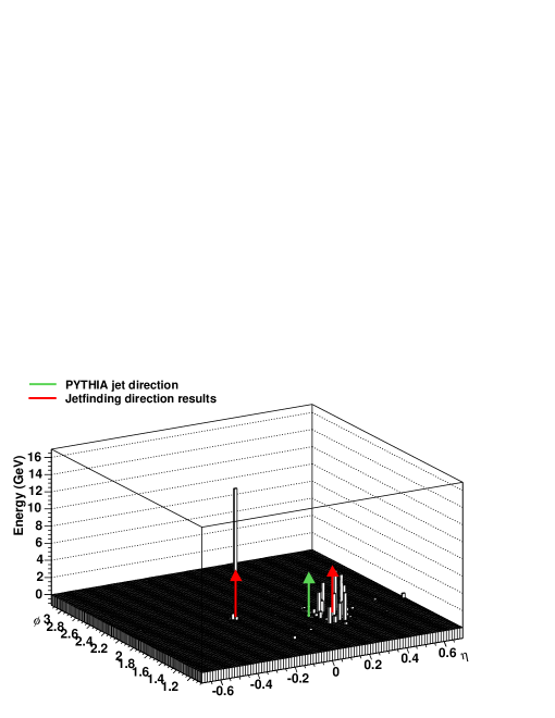
  Fig. 4.25: Grid energy including tracking and calorimetry information for a 100 GeV PYTHIA event where the algorithm reconstructed two jets (different event from that shown in Fig. 4.24). The green arrow indicates the direction of the trigger jet as calculated by PYTHIA and the red arrows indicate the directions of the two jets reconstructed by the algorithm.

  The figure shows the energy grid containing tracking and calorimetry information for a PYTHIA event containing a 100 GeV jet. The green arrow indicates the direction of the trigger jet as calculated by PYTHIA ($\eta$=0.17, $\phi$=1.80) and the red arrows show the directions of the two jets reconstructed by the seeded algorithm ($\eta_{1}$=-0.15, $\phi_{1}$=2.00) and ($\eta_{2}$=0.27, $\phi_{2}$=1.73). In this case, the reconstructed jet cone centres were an angular distance of $R=\sqrt{{(\Delta\eta)}^{2}+{(\Delta\phi)}^{2}}=0.50$ away from each other. If the energy weighted centroid of the two jets reconstructed by the algorithm is calculated, a direction coinciding with the jet direction calculated by PYTHIA is obtained. Therefore, the small cone radius of $R=0.3$ can lead to two jets being reconstructed where in fact there was only one. The proportion of events which contained two or more reconstructed jets and which satisfied the following conditions:

  1. (SC) $0.3<D<1.0$, where $D$ is the angular distance between the two reconstructed jets

  2. (SC) $\sqrt{(\eta_{PYTHIA}-\eta_{Weight})^{2}+(\phi_{PYTHIA}-\phi_{Weight})^{2}}<0.01$

  are shown in Table.4.10.

  	50 GeV Sample	75 GeV Sample	100 GeV Sample
  Percentage of events with $>1$ recon. jet and satisfying conditions 1(SC) $\&$ 2(SC)	0.02$\%$	0.11$\%$	0.35$\%$

  Table 4.10: Contribution to ‘fake’ rate from events containing 1 real PYTHIA jet which the jet-finding algorithm reconstructs as 2 jets due to the small cone size used ($R=0.3$).

• Algorithm and Physics Related Effects
  A combination of the physics involved and the nature of the jet finding algorithm may lead to the reconstruction of ‘fake’ jets. It has been found that cone jet finding algorithms, in which jet seeds are processed in decreasing order of $E_{T}$ and where a seed is removed from the list if it is included in a jet with a seed that is before it in the list, are sometimes sensitive to collinearity problems [51]. For example, Fig. 4.26 from [51] shows a situation at the parton level where the hardest parton in the jet (left-hand picture) splits into two almost collinear partons (right-hand picture). In both cases the same jet should be reconstructed, but if the $E_{T}$ ordered seed algorithm is used, different jets are reconstructed as shown by the different cone positions in the figure. In the case of the left-hand picture, the central parton will be treated as a seed by the algorithm first as it has the highest energy and all three partons will be grouped together in the jet and the others removed from the seed list. However, for the case in the right-hand picture, if the central parton splits such that one of the other two original partons have a higher energy than each of the split partons, then the algorithm could find a jet that excludes the third original parton as it could fall outside the chosen cone radius, $R$.

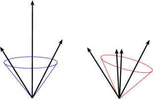
Fig. 4.26: Collinear partons (right-hand picure) resulting from the splitting of the central highest energy parton (left-hand picture) result in different jets being reconstructed by a jet finding algorithm with $E_{T}$ ordered seeds. The length of the parton arrows represent their relative $E_{T}$. From [51].

Event Type		$\epsilon$	Events with 0 reco. jets ($\%$)	Events with 1 reco. jet ($\%$)	Events with 2 reco. jets($\%$)	Events with $>$ 2 reco. jets($\%$)
Seeded algorithm,	50 GeV	0.862	25.5	63.9	9.69	0.958
combined events	75 GeV	1.11	6.70	76.7	15.2	1.39
	100 GeV	1.21	2.82	75.4	19.8	1.99
Seeded algorithm,	50 GeV	0.703	30.1	69.6	0.345	0.000
PYTHIA events	75 GeV	0.956	8.16	88.1	3.76	0.000
alone	100 GeV	1.05	3.45	87.9	8.54	0.0745
Seeded algorithm,	50 GeV	0.735	33.4	60.2	6.01	0.414
combined events,	75 GeV	0.996	12.0	77.3	9.68	0.958
tracking data only	100 GeV	1.09	6.66	79.0	13.3	1.10
Seedless algorithm,	50 GeV	2.40	0.603	19.5	37.4	42.5
combined events	75 GeV	2.46	0.0905	18.7	35.9	45.3
	100 GeV	2.50	0.135	17.5	36.0	46.4
Seedless algorithm,	50 GeV	0.835	16.5	83.4	0.0481	0.000
PYTHIA events	75 GeV	1.01	2.50	94.1	3.42	0.0113
alone	100 GeV	1.09	0.713	89.7	9.49	0.0566
Seeded algorithm, Central HIJING events alone		-	84.0	14.7	1.08	0.215
Seedless algorithm, Central HIJING events alone		-	15.5	31.4	29.0	24.1

Table 4.11: Efficiency results for the jet finding algorithm in its seeded and seedless versions for different input event types. Also shown is the fraction of events with no jets reconstructed, 1 jet only, 2 jets only, and greater than 2 jets reconstructed for the different input event types.

Table 4.11 shows the efficiency of the algorithm in its seeded and seedless versions for different event types. From Table 4.11, a general trend that can be seen is that the value of $\epsilon$ increases with increasing input jet energy for all event types. The definition of $\epsilon$ for Central HIJING events has no physical meaning in this case because the number of known input jets is zero. Another general trend is that all the $\epsilon$ values for 100 GeV jet cases are greater than 1, implying that the algorithm reconstructs more jets than are input for these cases. The values of $\epsilon$ for the seeded algorithm for pure PYTHIA events with no background, are within $5\%$ of the ideal value of 1 for 75 GeV and 100 GeV jets, however the efficiency is smaller, $\epsilon=0.7$, for the 50 GeV jets.

The seeded algorithm applied to combined events, with tracking plus calorimetry data, produces values of $\epsilon$ close to unity ($\pm 21\%$) although $\epsilon<1$ for the 50 GeV input jets implies that some real jets were excluded by the algorithm. These efficiency values are larger than those obtained from the seeded algorithm applied to the combined events with only tracking data.

The seedless algorithm, when applied to PYTHIA events with no background, produced values of $\epsilon$ ranging from $19\%$ greater (for the 50 GeV case) to $4\%$ greater (for the 100 GeV case) than the seeded algorithm values for pure PYTHIA events. Furthermore, the seedless algorithm found on average more than double the number of jets than were input for all input jet energies for combined events.

The third column of Table 4.11 shows the number of events for each case where no jets were reconstructed i.e. the algorithm failed to reconstruct a jet since the jet did not satisfy the algorithm cuts. Note that the values of $\epsilon$ in column two are calculated on an overall per input jets basis and the values in column three on a per event basis. Therefore the values in columns two and three are not expected to sum to unity. The percentage of events in which no jet was found decreases as a function of increasing jet energy since the algorithm parameters were optimised for 50 GeV jets. Therefore the higher energy jets which result in higher tower energies above the background, are easier to reconstruct. The jet exclusion rates are within $5\%$, but slightly lower than was predicted in Tables 3.1 and 3.2. The resulting exclusion rate obtained with the seeded algorithm on combined events is smaller than the rate obtained for pure PYTHIA events. This indicates that some ‘fake’ jets are reconstructed for the combined events since the jet signal is the same for the two cases and the only difference is the addition of background for the combined event. The seeded algorithm applied to combined events with only tracking data excludes a larger fraction of real jets than the other two cases. Since the calorimetry data is absent in this analysis while the parameters are optimised for the use of both tracking and calorimetry data, it is expected that the energy cuts on JetESeed and MinJetEt in the algorithm will exclude more jets.

In comparison, the seedless algorithm applied to pure PYTHIA events reconstructs more jets than the seeded algorithm. When it is applied to combined events, an $\epsilon$ is obtained which is double that obtained when it is applied to pure PYTHIA events. This is due to reconstruction of ‘fake’ jets because of the zero cut on JetESeed. This is also clear from the low percentage ($<$20$\%$) of these events where only one jet was reconstructed (column 4) compared to the case for the seeded algorithm on combined events ($>$60$\%$).

For the case of Central HIJING events alone which serve here as an estimate of the background, the seeded algorithm excludes a much larger percentage of events (84$\%$) than the seedless algorithm (16$\%$). Since, in this thesis, all reconstructed jets which are not from the PYTHIA signal, are classified as ‘fakes’, this indicates that the seeded algorithm is preferable to use since it excludes more background events.

The seeded algorithm, for all cases except background events, reconstructs a single jet per event for more than $60\%$ of events. On the other hand, less than $20\%$ of combined events are reconstructed as single jet events by the seedless algorithm which is more than three times lower than the case for the seeded algorithm.

The ‘fake’ rate for the algorithm in its seeded and seedless versions for the various input jet event types can be found from the percentage of input events where two or more jets are reconstructed i.e. by summing columns 5 and 6 in Table 4.11. The ‘fake’ rate for the seedless algorithm on combined events is greater than $80\%$ while the seeded algorithm on combined events (tracks plus calorimetry and tracks alone) produces a ‘fake’ rate of less than $22\%$. For the case of PYTHIA events alone, both the seeded and seedless algorithms produce a ‘fake’ rate of less than $10\%$ over all the input jet energies. For the case of Central HIJING events alone, the ‘fake’ rate of the algorithm can be found from the percentage of events where at least 1 jet is reconstructed because any jet reconstructed in a Central HIJING event is classified as a ‘fake’ jet here. Therefore, by summing columns 4, 5 and 6 in Table 4.11 for the cases of Central HIJING events alone, the ‘fake’ rate amounts to $85\%$ for the seedless algorithm and $16\%$ for the seeded algorithm ($2.8\%$ higher than predicted in Table 3.3). In conclusion, this investigation shows that the seeded algorithm is better to use than the seedless version since it reconstructs far fewer ‘fake’ jets resulting in a purer sample of real reconstructed jets.

4.3.2 ‘Fake’ Jet Reconstruction

In order to understand better the primary source of the ‘fake’ jets that were reconstructed, jet energy histograms were plotted for the second highest energy jet in events where two or more jets were reconstructed. Figs. 4.27 and 4.28 show a comparison of ‘fake’ and real jets for the seeded algorithm applied to 50 GeV combined events and 100 GeV combined events respectively. In Figs. 4.27 and 4.28 the blue histogram represents the second highest energy jet for events where two or more jets were reconstructed. The green histogram represents the energy of the highest energy jet per event for the same case. The red histogram represents the highest energy jet for all events where only one jet was reconstructed and the black histogram is the sum of the red and green histograms i.e. the energy distribution of the highest energy jet found in all events (the same as shown in Figs. 4.1 and 4.3 respectively). The same cases are plotted for the seedless algorithm applied to 50 GeV combined events and 100 GeV combined events and are shown in Figs. 4.29 and 4.30 respectively. The proportion of events where a second jet (‘fake’) was reconstructed is much larger when the seedless algorithm is used as shown in Figs. 4.29 and 4.30 compared to Figs. 4.27 and 4.28.

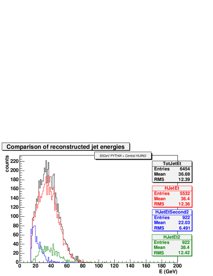
Fig. 4.27: Comparison of reconstructed jet energies for different cases for 50 GeV combined events and the seeded algorithm. The blue histogram shows the second highest energy jet and the green shows the highest energy jet for events where two or more jets were reconstructed. The red histogram shows the highest energy jet for events where only one jet was reconstructed. The black histogram shows the distribution for the highest energy jet for events where at least one jet was reconstructed (the sum of the red and green histograms).

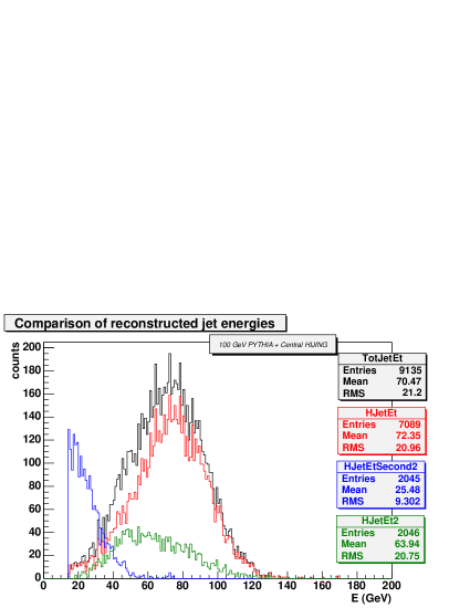
Fig. 4.28: Comparison of reconstructed jet energies for different cases for 100 GeV combined events and the seeded algorithm. The colours represent the same quantities described in Fig. 4.27.

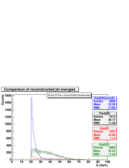
Fig. 4.29: Comparison of reconstructed jet energies for different cases for 50 GeV combined events and the seedless algorithm.The colours represent the same quantities described in Fig. 4.27.

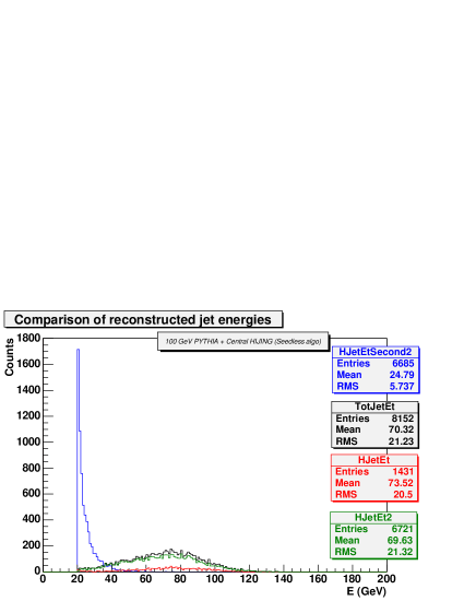
Fig. 4.30: Comparison of reconstructed jet energies for different cases for 100 GeV combined events and the seedless algorithm.The colours represent the same quantities described in Fig. 4.27.

For comparison the energy distributions of jets reconstructed using the seeded algorithm (red) and the seedless algorithm (blue) in Central HIJING events, are shown in Fig. 4.31. Again more ‘fakes’ are reconstructed by the seedless algorithm compared to the seeded algorithm.

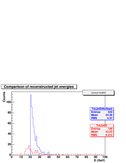
Fig. 4.31: Reconstructed jet energy distributions for Central HIJING events using the seeded algorithm (red) and the seedless algorithm (blue).

The top section of Table 4.12 shows the mean energies of the second highest energy jets reconstructed in events with at least two reconstructed jets for the cases of the seeded and seedless versions of the algorithm and the different input event types. The bottom section of the table shows the mean energy of the highest energy jets reconstructed using the seeded and seedless versions of the algorithm on Central HIJING events alone.

Data Type	$\langle E^{2nd}_{Reco}\rangle$ for 50GeV input (GeV)	$\langle E^{2nd}_{Reco}\rangle$ for 75GeV input (GeV)	$\langle E^{2nd}_{Reco}\rangle$ for 100GeV input (GeV)
Seeded algorithm, combined events	22.03	23.18	25.48
Seeded algorithm, PYTHIA events alone	16.60	21.22	25.22
Seedless algorithm, combined events	23.36	24.21	24.77
Seedless algorithm, PYTHIA events alone	20.82	23.69	26.95
Data Type	$\langle E^{1st}_{Reco}\rangle$ for all input events (GeV)
Seeded algorithm, Central HIJING events alone	23.23
Seedless algorithm, Central HIJING events alone	24.36

Table 4.12: The top section of the table shows the mean reconstructed energy for the second highest $E_{T}$ jets in events where at least two jets were reconstructed for the case of the seeded and seedless algorithm applied to different input event types. The lower section of the table shows the mean reconstructed energy for the highest $E_{T}$ jets for Central HIJING events alone, see Fig. 4.31.

It can be argued that the primary source of ‘fake’ jets is the background with its large event-by-event fluctuations. The evidence to suggest this is as follows: For both algorithms, in the case of combined events, the mean reconstructed jet energies for the second highest energy jets (per event) are closer to the value of the highest energy jets reconstructed in Central HIJING events, than is the case for PYTHIA events alone. For the seeded algorithm case, the reconstructed jet energies, $\langle E^{2nd}_{Reco}\rangle$, for the combined events are within $10\%$ of the $\langle E^{1st}_{Reco}\rangle$ for Central HIJING events while the reconstructed energies for PYTHIA alone differ by up to $30\%$. A similar trend is observed for the seedless algorithm case where for the combined events, $\langle E^{2nd}_{Reco}\rangle$ are within $4\%$ of the $\langle E^{1st}_{Reco}\rangle$ for Central HIJING while for PYTHIA events alone, the difference is up to $14\%$.

The ‘fake’ rates for PYTHIA events alone using both the seeded and seedless versions of the algorithm are very similar for respective input jet energies (see Table 4.11) but the addition of background to these events increases the ‘fake’ rates. The addition of background more than doubles the ‘fake’ rate for the case of the seeded algorithm on combined events. For the seedless algorithm, the ‘fake’ rate is more than ten times higher for combined events than for PYTHIA events alone. Therefore the primary source of ‘fake’ jets is due to contribution from the background or ‘underlying event’.

4.4 Energy Resolution

Fig. 4.32 compares the resulting jet energy resolutions obtained when using the seeded version of the algorithm on combined events with tracking data alone (represented by the open symbols) compared to tracking plus calorimetry data (represented by the solid symbols). The optimised algorithm parameters shown in Table  4.1 are used. The resolution, $\sigma/\langle E_{Fit}\rangle$, is calculated by dividing the $\sigma$ by the mean of the gaussian fitted reconstructed jet energy distribution. By using a combination of tracking and calorimetry information to reconstruct jets, an improvement of up to $54\%$ for the energy resolution of 50 GeV jets is obtained compared to using tracking information only. This brings the resolution of 50 GeV jets down from $93\%$ (tracking only) to $39\%$ (tracking plus calorimetry) and of 100 GeV jets from $54\%$ (tracking only) down to $30\%$ (tracking plus calorimetry).

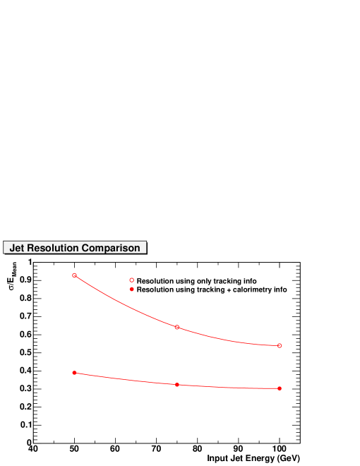
Fig. 4.32: Jet energy resolution ($\sigma/\langle E_{Reco}\rangle$) for combined events using the optimised seeded algorithm for events where only tracking information was used (open symbols) compared to when tracking plus calorimetry information was used (closed symbols).

The resolutions obtained using the seeded version of the algorithm compared to the seedless version are plotted in Fig. 4.33. The red lines indicate combined events (Pb+Pb) and the blue lines indicate pure PYTHIA events (p+p). In both the combined event and pure PYTHIA event cases, the seeded algorithm (solid symbols) produces lower resolutions than the seedless algorithm (open symbols). For the seeded algorithm (solid symbols), the resolutions obtained for combined events approach the values obtained for the pure PYTHIA case as a function of increasing jet energy.

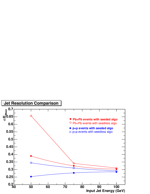
Fig. 4.33: Jet energy resolution ($\sigma/\langle E_{Reco}\rangle$) for combined events (red) compared to PYTHIA events alone (blue) using the seeded algorithm (solid symbols) compared to the seedless algorithm (open symbols).

Chapter 5 Conclusions

This thesis demonstrates the first successful attempt to reconstruct high-$p_{T}$ jets ($E_{Tjet}>50$ GeV) in high-multiplicity ($dN_{ch}/dy=4000$) heavy-ion collisions at $\sqrt{s_{NN}}=5.5$ TeV using a UA1-based cone algorithm modified for this purpose and detectors from the ALICE experiment at the LHC. The algorithm parameters were optimised for the heavy-ion environment and a method of calculating and subtracting the large background energy contribution on an event-by-event basis was developed in order to reconstruct the jet energy.

It has been shown that due to the large event-by-event background fluctuations, a small cone size of $R=0.3$ is required to optimise the measurement of the jet energy. The combination of information from the tracking detectors and the electromagnetic calorimeter produces much improved jet energy resolution results and more accurate jet direction reconstruction when compared to using tracking information alone. The shift towards lower energy of the reconstructed jet energies due to the small cone radius and other algorithm effects is understood and can be corrected for using a cross-section weighted multiplicative factor which is independent of jet energy (in the range 50 GeV/$c$$<E_{T}<$100 GeV/$c$).

The seeded algorithm is the preferred algorithm to use since it resulted in much lower ‘fake’ jet rates and better jet energy resolution than the seedless version. Artefacts of the algorithm such as the use of a small cone radius and jet-seed $E_{T}$ ordering contribute negligibly to the resulting ‘fake’ jet rates.

The jet finding algorithm detailed in this thesis is now ready for data analysis in the field of heavy-ion physics.

Appendix A Glossary of Terms

1. Jet
   A jet is a localised (in $\eta,\phi$-space) group of hadrons orginating from the fragmentation of a hard scattered parton.

2. Combined event
   An event consisting of a PYTHIA jet event superimposed on a HIJING background event.

3. PYTHIA
   A Monte Carlo event generator for the simulation of high energy physics events.

4. HIJING
   HIJING (Heavy Ion Jet Interaction Generator) is a Monte Carlo event generator based on PYTHIA for simulating A+A collisions.

5. Jet-finding algorithm parameters:
   

   1. Cone radius ($R$)
      The cone radius ($R=\sqrt{(\Delta\eta)^{2}+(\Delta\phi)^{2}}$) defines the angle from the jet axis within which energy will be measured when reconstructing jets according to the cone algorithm prescription.

   2. Track $p_{T}$-cut
      A threshold momentum which determines which tracks are included or excluded in the analysis.

   3. JetESeed
      The minimum energy a grid cell must have in order to be classified as a jet seed by the algorithm.

   4. MinJetEt
      The minimum energy contained within a cone to be classified as a jet by the algorithm.

6. Seeded algorithm
   The modified algorithm as presented here where the parameter $JetESeed>0$ GeV.

7. Seedless algorithm
   The modified algorithm as presented here where the parameter $JetESeed=0$ GeV.

8. ‘Real’ jet
   A ‘real’ jet is classified here as the PYTHIA jet in a combined event. This is the jet we aim to reconstruct in the analysis.

9. ‘Fake’ jet
   A ‘fake’ jet is defined here as any jet that is reconstructed by the algorithm but that is not the input PYTHIA jet.

Appendix B Reconstructed Jet Energy Fit Results

Data Type		$\langle E_{Reco}\rangle$ (GeV)	$\sigma$ (GeV)	$\chi^{2}/ndf$
Seeded algorithm,	50 GeV	33.54	14.17	86.61/68
combined events	75 GeV	51.62	17.53	207.6/100
	100 GeV	69.33	22.03	295.8/124
Seeded algorithm,	50 GeV	13.56	12.59	37.82/40
combined events,	75 GeV	27.01	17.35	87.96/70
tracking data only	100 GeV	39.25	21.18	73.52/94
Seeded algorithm,	50 GeV	32.04	8.10	192.2/48
PYTHIA events	75 GeV	48.67	13.51	252.9/82
alone	100 GeV	65.90	18.71	268.9/112
Seedless algorithm,	50 GeV	26.10	17.15	98.27/64
combined events	75 GeV	51.58	17.57	140.7/92
	100 GeV	69.71	21.59	220.6/116
Seedless algorithm,	50 GeV	28.15	9.70	95.07/42
PYTHIA events	75 GeV	46.82	14.50	311.3/75
alone	100 GeV	65.29	19.04	300.8/107

Table B.1: Reconstructed jet energy fit parameters for various event and algorithm types.

Bibliography

- [1]
- [2] J. C. Collins and M. J. Perry, Phys. Rev. Lett. 34, 1353 (1975)
- [3] F. Karsch, Nucl. Phys. A 698, 199c (2002)
- [4] D. H. Perkins, Introduction to High Energy Physics, Cambridge University Press (2000)
- [5] D. Gross and F. Wilczek, Phys. Rev. Lett. 30, 1343 (1973)
- [6] H. D. Politzer, Phys. Rev. Lett. 30, 1346 (1973)
- [7] J. Phys. G: Nucl. Part. Phys. 30, Proceedings of Quark Matter 2004 Conference, Oakland, USA (2004) and references therein
- [8] Z. Fodor, Nucl. Phys A 715, 319c (2003)
- [9] C. Wong, Introduction to High-Energy Heavy-Ion Collisions, World Scientific (1994)
- [10] K. Rajagopal and F. Wilczek, hep-phy/0011333
- [11] J. W. Harris and B. Muller, Annu. Rev. Nucl. Part. Sci. 46:71-107 (1996)
- [12] G. F. Chapline et al, Phys. Rev. D 8, 4302 (1973)
- [13] N. Xu and M. Kaneta, Nucl.Phys. A 698, 306, (2002)
- [14] J. Cleymans and K. Redlich, Phys. Rev. C60, 054908, (1999)
- [15] P. Braun-Munzinger et al. Phys. Lett. B 518 41 (2001)
- [16] K.J. Eskola and K. Kajantie, Z. Phys. C75, 515 (1997)
- [17] T. Matsui and H Satz, Phys Lett B 178, 416 (1986)
- [18] J. Rafelski, Phys. Rep. 88, 331 (1982)
- [19] R. D. Pisarski Phys. Lett. B 110, 155 (1982)
- [20] X-N. Wang, Phys. Rep. 280, 287 (1997)
- [21] M. Strickland, Phys. Lett. B 331, 245 (1994)
- [22] J.L. Klay, Private Communication
- [23] X-N. Wang and M. Gyulassy, Phys. Rev. Lett. 68, 1480 (1992)
- [24] X-N. Wang, Z. Huang and I. Sarcevic, Phys. Rev. Lett. 77, 231 (1996)
- [25] C. A. Salgado and U. A. Wiedemann, hep-ph/0310079
- [26] G. Arnison, et al, Phys. Lett. B 132, 223 (1983)
- [27] U.A. Wiedemann and A. Morsch, Private communication
- [28] T. Sjostrand et al, Computer Physics Commun. 135, 238 (2001)
- [29] X.N.Wang and M.Gyulassy, Phys. Rev. D 44, 3501 (1991)
- [30] M. J. Horner, Private communication
- [31] W. Barletta et al., Nucl. Instr. and Meth. Special Issue A499, (2003)
- [32] C. Adler et al, Phys. Rev. Lett. 89 202301 (2002)
- [33] J. Adams et al, Phys. Rev. Lett 91 172302 (2003)
- [34] S.S. Adler et al, nucl-ex/0308006
- [35] C. Adler et al, Phys. Rev. Lett. 90, 082302 (2003)
- [36] J. Adams et al,Phys. Rev. Lett. 91, 072304 (2003)
- [37] S.S. Adler et al, Phys. Rev. Lett. 91, 072303 (2003)
- [38] F. Wang, Measurement of jet fragmentation at RHIC, Talk at Quark Matter Conference (2004)
- [39] M. Gyulassy and I. Vitev, Quark Matter Conference (2002)
- [40] K.J. Eskola et al, Nucl. Phys. A 696, 715 (2001)
- [41] A. Accardi et al, Preprint hep-ph/0310274
- [42] ALICE-USA collaboration, Proposal for Electromagnetic Calorimeter for ALICE at the LHC (2003)
- [43] ALICE Collaboration: F Carminati et al, J. Phys. G: Nucl. Part. Phys. 30, 1517 (2004)
- [44] A. Akopian, CDF PhD Thesis, The Rockefeller University, (1999), unpublished
- [45] W.Christie and K Shestermanov, STAR Note 196 (1995), unpublished
- [46] ALICE website, http://alice.web.cern.ch
- [47] ALICE Collaboration: F Carminati et al, ALICE PPR Volume II, (2003), unpublished
- [48] P. Glassel, The ALICE TPC - an innovative device for heavy ion collisions at LHC, Talk at Quark Matter Conference (2004)
- [49] S.D. Ellis, D.E. Soper, Phys. Rev. D 48, 3160 (1993)
- [50] G. Sterman and S. Weinberg, Phys. Rev. Lett. 39, 1436 (1977)
- [51] Gerald C. Blazey et al, hep-ex/0005012 v2
- [52] G. Arnison, et al, Phys. Lett. B 132, 214 (1983)
- [53] S.D. Ellis, et al, Research Directions for the Decade, Proceedings of the Summer Study, Snowmass, Colorado, 1990, edited by E.L. Berger (World Scientific, Singapore, 1992), p134
- [54] A. Bocci, CDF PhD Thesis, University of Pisa (1998), unpublished
- [55] J. Dittmann, CDF PhD Thesis, (1998), unpublished
- [56] T. Affolder et al., Phys. Rev. D 65, 092002 (2002)
- [57] G. Latino, CDF PhD Thesis, Casino (2001), unpublished
- [58] D. Buskulic et al, Nucl. Instr. and Meth. in Physc. Res. A 360 (1995)
- [59] S.Lami et al FERMILAB-CONF-00/342-E, Published Proceedings 9th Conference on Calorimetry in High Energy Physics (CALOR 2000), Annecy, France, October 9-14, 2000
- [60] C. Adler et al, Phys. Rev. Lett. 90, 032301 (2003)
- [61] G. Arnison, et al, Phys. Lett. B 118, 173 (1982)
- [62] ALICE-USA Collaboration, LBL Workshop, January (2003)
- [63] http://aliweb.cern.ch/offline/
- [64] Application Software Group, CERN Program Library Long Writeup W5013
- [65] W. R. Leo, Techniques for Nuclear and Particle Physics Experiments, Springer-Verlag (1987)
- [66] T. Sjostrand et al, hep-ph/0108264 (2002)
- [67] H. Gray, Private communication