Near threshold $\eta$ meson production in the ${dd}\,\to\,^{4}\mathrm{He}\,\eta$ reaction

Abstract

The ${dd}\,\to\,^{4}\mathrm{He}\,\eta$ reaction has been investigated near threshold using the ANKE facility at COSY–Jülich. Both total and differential cross sections have been measured at two excess energies, $Q=2.6$ MeV and 7.7 MeV, with a subthreshold measurement being undertaken at $Q=-2.6$ MeV to study the physical background. While consistent with isotropy at the lower energy, the angular distribution reveals a pronounced anisotropy at the higher one, indicating the presence of higher partial waves. Options for the decomposition into partial amplitudes and their consequences for determination of the $s$-wave $\eta$-$\alpha$ scattering length are discussed.

1 Introduction

Interest in the physics of the $\eta$ meson underwent a revival in the 1980s when it was discovered that the $\eta$–nucleus interaction is so strong and attractive that the existence of $\eta$–nucleus quasi–bound states was hypothesised Liu86 ; Haider86 ; Chiang91 . The original predictions of such states concerned heavier nuclei ($A>11$) but direct searches for them in the cases of lithium, carbon, oxygen and aluminium proved inconclusive Chrien88 ; Lieb00 . More recent theoretical approaches, using more attractive $\eta$–nucleus interactions, gave positive predictions for much lighter nuclei, e.g. the helium isotopes Wilkin93 ; Wycech95 ; Fix02 ; Rakityansky95 ; Rakityansky96 . Data on the ${pd}\,\to\,^{3}\mathrm{He}\,\eta$ and ${dd}\,\to\,^{4}\mathrm{He}\,\eta$ reactions obtained at the SATURNE accelerator Berger88 ; Mayer96 ; Frascaria94 ; Willis97 and other laboratories Betigeri00 ; Bilger02 ; Adam05 have been interpreted by some authors as suggesting that the $\eta$–⁴He, and perhaps even $\eta$–³He, systems could support bound states Willis97 ; Tryasuchev97 . Attempts have also been made to photoproduce the latter Pfeiffer , though the analysis is not completely unambiguous Hanhart:2004qs .

It is important to stress that $\eta$–nucleus bound states should first occur in the $s$-wave. Thus, any calculation exploiting information extracted just from total cross sections relies on the implicit assumption of purely $s$-wave production in the proximity of the reaction threshold. Verification of this assumption requires the measurement of angular distributions and polarisation observables as well as total cross sections. Differential cross sections do exist for ${pd}\,\to\,^{3}\mathrm{He}\,\eta$ close to threshold Mayer96 ; Betigeri00 ; Bilger02 ; Adam05 , and these indicate the onset of higher partial waves at $Q\approx 15$ MeV. For the ${dd}\,\to\,^{4}\mathrm{He}\,\eta$ process, data on the total cross section are restricted to small excess energies ($Q<9$ MeV) and no data whatsoever are available on differential cross sections.

2 Experiment

The experiment Wronska05 , aiming at the determination of total cross sections and angular distributions for ${dd}\,\to\,^{4}\mathrm{He}\,\eta$ close to threshold, was performed in the Institut für Kernphysik of the Forschungszentrum Jülich. The measurement was carried out at the ANKE facility Barsov01 , located at an internal target position of the COSY synchrotron, for three beam momenta, 2.328 GeV/c, 2.343 GeV/c and 2.358 GeV/c. The first of these lies below the reaction threshold and was undertaken to study the shape of the physics background. The other two correspond to excess energies of 2.6 MeV and 7.7 MeV, respectively. With around $5\times 10^{10}$ deuterons circulating in the COSY ring and a D₂ cluster jet target target , a luminosity of about $4\times 10^{30}$ s^-1cm^-2 was achieved.

The measurement assumed detection of ${}^{4}\mathrm{He}$ particles and reconstruction of their momenta, followed by a missing–mass analysis of the remaining reaction products. The detection system was based on three magnets D1-D3 forming a chicane in the COSY ring (full setup is presented e.g. in fig.2 of Barsov01 ), with the target position located between D1 and the spectrometer magnet D2. In the layout used in the experiment (see fig. 1), only the forward detection system located between the D2 and D3 magnets was exploited. This comprised two multiwire drift chambers (MWDC) for track reconstruction and three layers of the scintillation hodoscope allowing time–of–flight and energy–loss determinations.

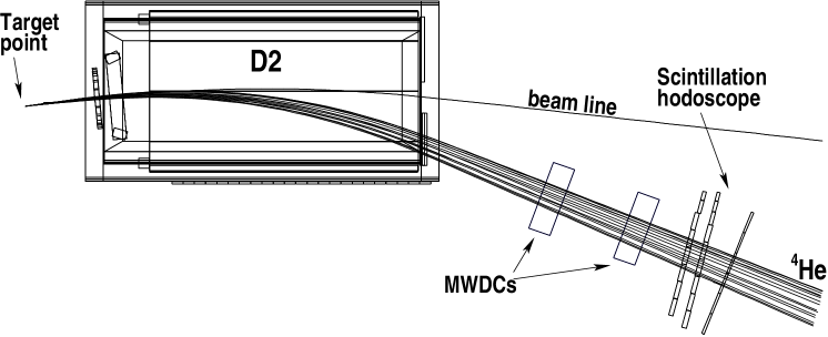
Figure 1: Layout of the forward detection system of ANKE used in the experiment. Several trajectories of $\alpha$-particles originating from the ${dd}\,\to\,^{4}\mathrm{He}\,\eta$ reaction are depicted.

Simulations showed that the ANKE acceptance is nearly 100% up to $Q\approx 6.6$ MeV and full coverage in polar angle is assured up to $Q\approx 90$ MeV. The angular resolution (in cms) for the $\alpha$-particles stemming from ${dd}\,\to\,^{4}\mathrm{He}\,\eta$ was determined to be not worse than 19^∘ for the lower energy ($Q_{1}$) and 11^∘ for the higher ($Q_{2}$). Moreover, the resolution in the transverse momentum component was about four times better than that of the longitudinal component. Thus, investigation of the transverse momentum spectrum provides direct information on the excess energy.

The application of a dedicated energy–loss–based trigger was necessary in order to obtain satisfactory background suppression for the data acquisition system. Since all scintillation counters were read out from both sides, this required special integrating modules, allowing summation and integration of two analogue signals. The discrimination threshold was set below the $\Delta E$–$p$ band of the ${}^{3}\mathrm{He}$. Additionally, a sample of data was collected with a minimum bias trigger.

There was strong contamination in the raw data from protons resulting from deuteron break-up since these have rigidities very close to those of the ${}^{4}\mathrm{He}$ particles of interest. In order to ensure a clean selection of ${}^{4}\mathrm{He}$ events, it was necessary to apply cuts on all $\Delta E_{i}$–$p$ spectra ($i=1,2,3$) and $T_{j1}$–$p$ ($j=2,3)$ with the reference time being given by the signal from the first hodoscope layer. The cut shapes were determined by dividing the three-dimensional spectra into slices and fitting the contents with Gaussians. The cut widths were taken to be at least three standard deviations and, in case of ambiguities (in the region of the break-up background), the width was interpolated between neighbouring regions with lower background content. Typical shapes of the cuts applied are shown in fig. 2.

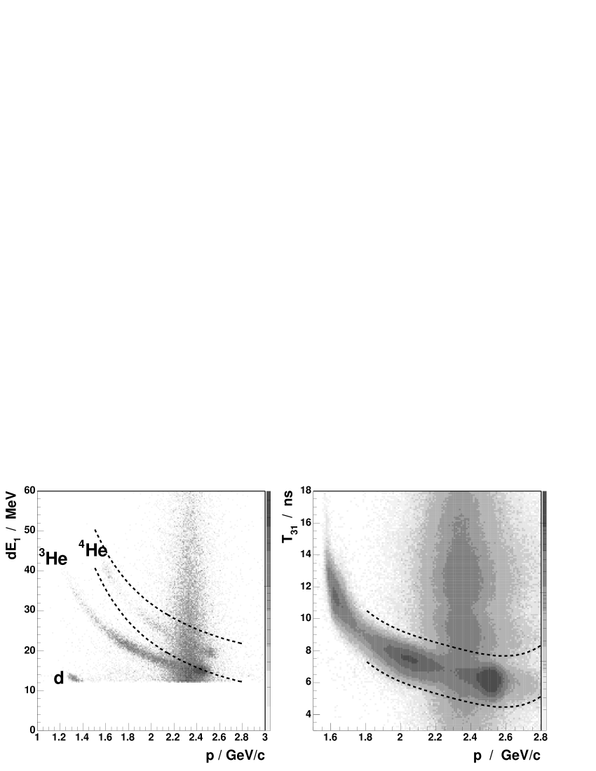
Figure 2: Typical shapes of the $\Delta E_{i}$–$p$ (left) and $T_{j1}$–$p$ (right) cuts applied in the selection of the ${}^{4}\mathrm{He}$ particles.

The overall suppression factor from minimum bias trigger to software ${}^{4}\mathrm{He}$ selection amounted to about $10^{5}$. The final momentum spectrum depicted in fig. 3 exhibits a three–peak structure, similar to those reported in ref. Banaigs76 . This is a reflection of the well–known ABC effect ABC , which leads to kinematic enhancements of the two–pion mass spectrum at both small masses (the outer peaks) and at maximum mass (the central peak) GFW .

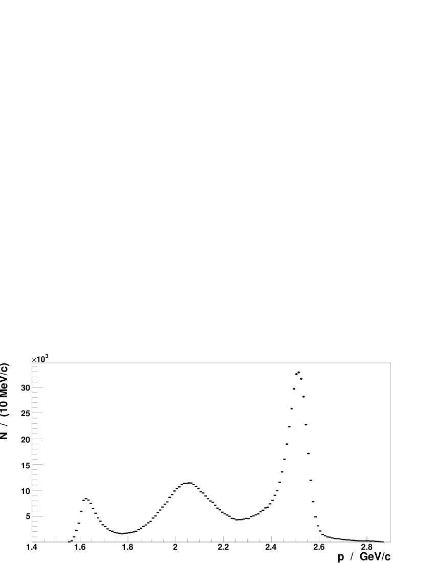
Figure 3: Inclusive momentum distribution of ${}^{4}\mathrm{He}$ particles measured at excess energy $Q_{1}$.

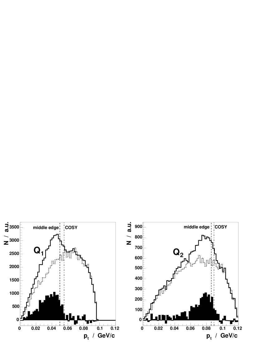
Figure 4: Distributions of transverse momenta of identified $\alpha$–particles obtained for nominal beam momenta of 2.345 GeV/c (left, solid line) and 2.360 GeV/c (right, solid line) for events with $m_{X}>0.54$ GeV/c². On top of them the phase-space-scaled subthreshold data are drawn with dotted lines. The difference, corresponding to events just with $\eta$ production, is represented by filled histograms. Vertical lines indicate $p_{\mathrm{cm}}$ calculated from the nominal beam momenta and that deduced from the presented spectra.

The solid lines in fig. 4 represent data obtained above threshold at $Q_{1}$ and $Q_{2}$ while the dotted lines indicate background. For both of the energies studied the background measured at $Q_{0}$ was scaled according to the available phase space and luminosity ratio Hibou99 , the latter being determined from the ratio of the histogram sums outside of the $\eta$ peak region. The filled histograms result from subtraction of the background spectra and should thus represent pure $\eta$ signals.

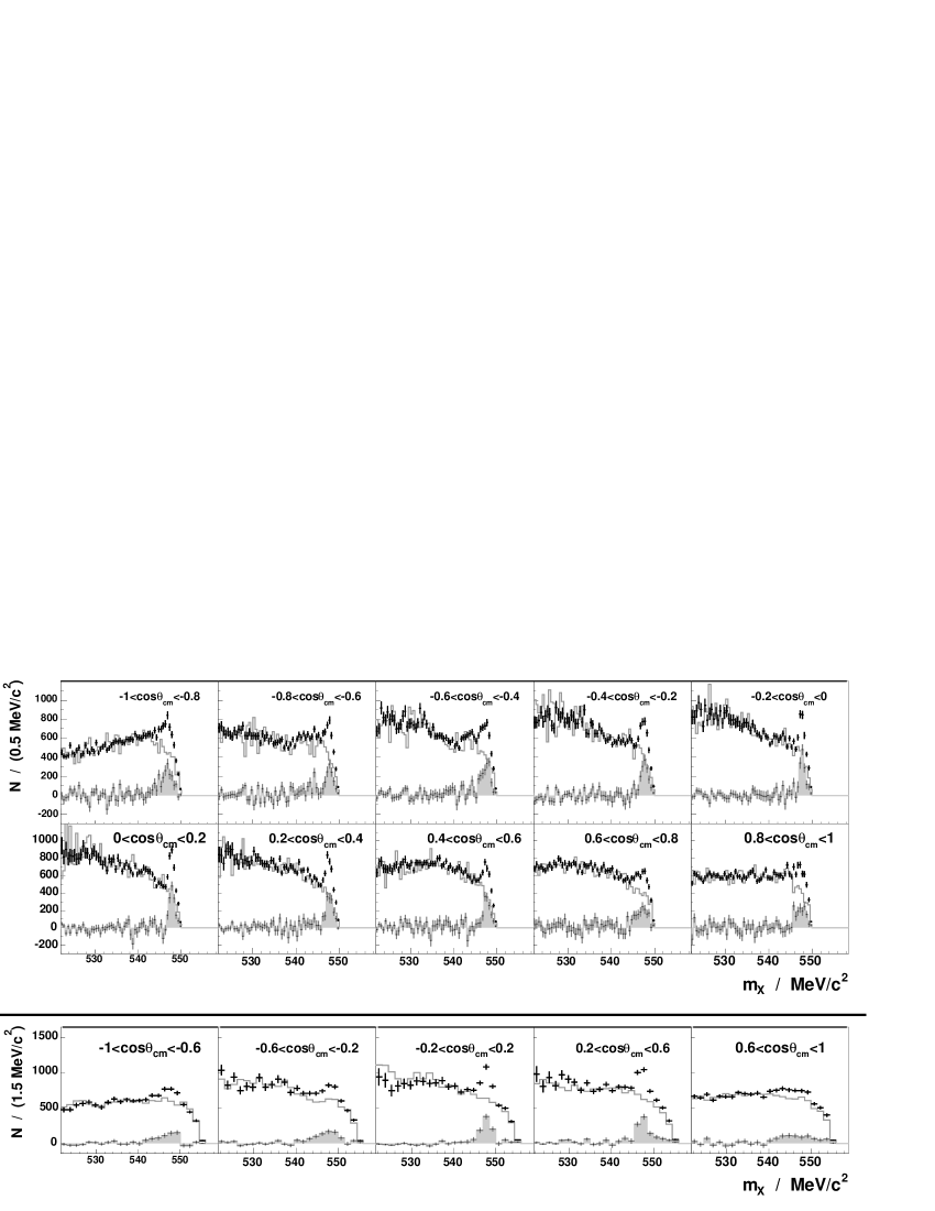
Figure 5: Missing-mass distributions for the ${dd}\,\to\,^{4}\mathrm{He}\,{X}$ reaction in bins of cms angle at excess energies $Q_{1}$ (upper panels) and $Q_{2}$ (lower panels). The scaled background, shown by the grey lines, is subtracted from the data to leave the desired $\eta$ peaks.

Analysis of the transverse momentum spectra shown in fig. 4 provides information on the cms momentum of the outgoing particles, and thus the excess energy which does not rely on knowing the mass of the $\eta$–meson precisely. The simulations show that the final cms momentum can be determined from the middle of the steeper edge of the transverse momentum distributions. In the left panel of fig. 4, the middle of the edge occurs at 50 MeV/c rather than 55 MeV/c, as calculated from the nominal beam momentum using the GEM value of $m_{\eta}$ gem05 . This difference, which depends upon the assumed value of $m_{\eta}$, indicates that the real beam momentum in the $Q_{1}$ case was about 2 MeV/c lower than the nominal value, which is within the precision of the absolute COSY settings. The relative beam momenta are, however, known with an order of magnitude better precision so that the shift found at $Q_{1}$ was assumed to be valid also at the other two energies. The spectra on the right of fig. 4 do not contradict this hypothesis.

The deduced values of the cms momenta and the corresponding excess energies are:

$$Q_{0}=(-2.6\pm 0.6)\textrm{ MeV ,}$$

$$p_{\mathrm{cm,1}} =(50\pm 5)\textrm{ MeV/c,~{}~{}~{}} Q_{1}=\phantom{-}(2.6\pm 0.6)\textrm{ MeV,}$$

$$p_{\mathrm{cm,2}} =(86\pm 4)\textrm{ MeV/c,~{}~{}~{}} Q_{2}=\phantom{-}(7.7\pm 0.8)\textrm{ MeV.}$$

Acceptance and resolution corrections were determined through GEANT simulations geant3 , taking into account the influence of physics processes (small angle scattering, energy loss, etc.) as well as the setup features (geometry, extended target, finite position resolution of the MWDCs, etc.). The acceptance $A(m_{X},\cos\theta_{\mathrm{cm}})$ was expressed in terms of the missing mass and the cosine of the cms polar angle. As starting values, we used data on inclusive ${}^{4}\mathrm{He}$ production in $dd$ collisions Banaigs76 but, to ensure good statistics also in the cells that were poorly populated in the event generator, this was supplemented with a sample of uniformly distributed events. For the total event distribution this introduces only a small change, but it helps significantly in the reduction of the final statistical uncertainty. For the above-threshold energies, separate samples of isotropically produced $\eta$ events were generated, but these were only used to correct the angular distributions.

To find the angular distributions of the ${}^{4}\mathrm{He}$ from the ${dd}\,\to\,^{4}\mathrm{He}\,\eta$ reaction, events were divided into angular bins and missing mass spectra were considered separately for each bin, the scaled background events being treated in the same way. For the lower energy above threshold, the statistics allowed a division into ten angular bins of equal width in $\cos\theta_{\mathrm{cm}}$. For the higher energy, where the statistics and missing mass resolution were several times worse, the data were divided into five intervals. In the results, shown in fig. 5, the background is corrected using the ${dd}\,\to\,^{4}\mathrm{He}\,{X}$ simulation. The resulting subtracted spectra should represent pure $\eta$ signals (filled histograms in fig. 5) though influenced by acceptance and resolution. The effects of these were unfolded using information from the simulation of ${dd}\,\to\,^{4}\mathrm{He}\,\eta$ events.

The total luminosities were estimated by comparing data with the inclusive differential ${dd}\,\to\,^{4}\mathrm{He}\,{X}$ results of ref. Banaigs76 , which have an absolute uncertainty of about 15%. The central bump in the three–peak structure of the ${}^{4}\mathrm{He}$ momentum distribution was parametrised by a Gaussian with parameters depending on the polar angle and beam momentum. The integrated luminosities for the three excess energies were:

$$L_{0} = \phantom{1}(316\pm 3_{\mathrm{\,stat}})\,\textrm{nb}^{-1}\>,$$

$$L_{1} = (1566\pm 21_{\mathrm{\,stat}})\,\textrm{nb}^{-1}\>,$$

$$L_{2} = \phantom{1}(299\pm 5_{\mathrm{\,stat}})\,\textrm{nb}^{-1}\>.$$

As checks on the luminosity, values were also determined from yields of the ${dd}\,\to\,^{3}\mathrm{He}\,{n}$ reaction compared with the published data of ref. Bizard80 , the event selection and acceptance correction being performed in a way similar to that described for ${}^{4}\mathrm{He}$. The numbers obtained from this analysis (317 nb^-1, 1425 nb^-1 and 255 nb^-1 at the three energies) are consistent with those determined from the ${dd}\,\to\,^{4}\mathrm{He}\,{X}$ data within the overall uncertainties. However, the latter reaction is preferable for our purposes since it involves the detection of ${}^{4}\mathrm{He}$ particle with momenta similar to those arising from ${dd}\,\to\,^{4}\mathrm{He}\,\eta$. By normalising to the ${dd}\,\to\,^{4}\mathrm{He}\,{X}$ process, uncertainties originating from the detection setup efficiency cancel completely and those in the acceptance at least partially.

3 Results

The analysis of the experimental data presented in the previous section yielded the following total cross sections

$$\sigma_{1} = \left(13.1\pm 0.7_{\mathrm{\,stat}}\pm 1.8_{\mathrm{\,syst}}\right)\>\textrm{nb}\>,$$

$$\sigma_{2} = \left(16.4\pm 1.0_{\mathrm{\,stat}}\pm 2.1_{\mathrm{\,syst}}\right)\,\textrm{nb}\>.$$ (3.1)

The systematic errors quoted here have been estimated by varying the conditions of the analysis within their uncertainties and do not include the 15% uncertainty in the luminosity, which does not affect the relative size of the cross section at the two energies.

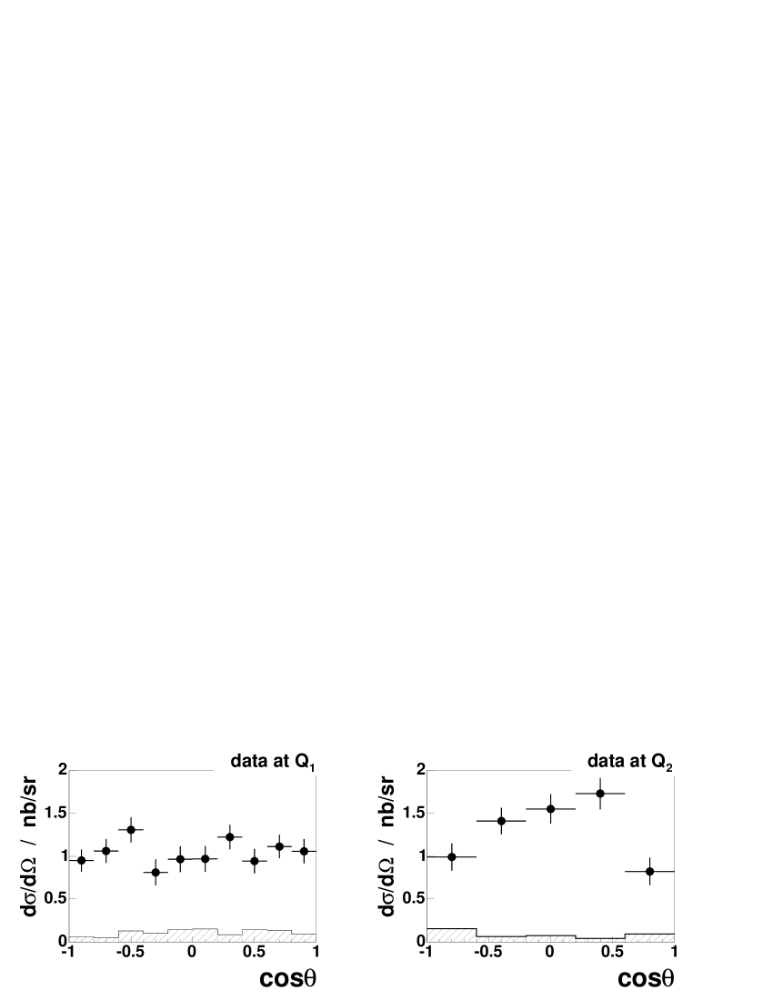
Figure 6: Experimental angular distributions of the ${dd}\,\to\,^{4}\mathrm{He}\,\eta$ reaction at the two excess energies. The error bars attached to the points are statistical, while the systematic ones are drawn as histograms.

Of the corresponding angular distributions depicted in fig. 6, the one obtained at excess energy $Q_{1}$ appears isotropic, whereas that at $Q_{2}$ reveals a strong angular dependence. Due to the identical nature of the deuterons in the initial state, the cross section must be symmetric in $\cos\theta$ and our results are consistent with this within the error bars.

In order to quantify the results, both angular distributions were each fitted with two functions: a constant $\textit{Pol0}(\cos\theta)=C_{0}$ and a symmetric second order polynomial $\textit{Pol2}(\cos\theta)=C_{0}\,\left(1+C_{2}\cos^{2}\theta\right)$. For fitting purposes, statistical and angular-dependent systematic errors were added in quadrature. The resulting fitted curves are superimposed on the experimental data in fig. 7 while the values of the parameters are collected in table 1. From this procedure it is clear that at the higher energy there is a significant negative value for $C_{2}$.

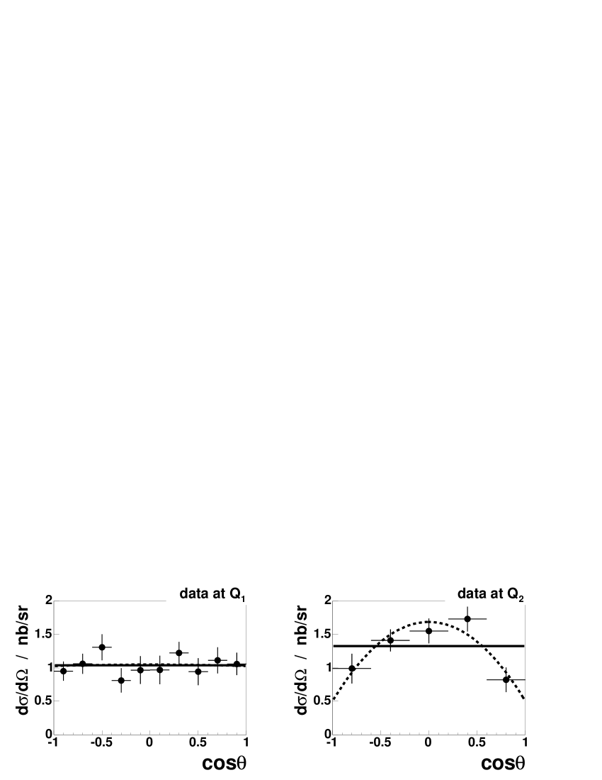
Figure 7: Fits of a constant and a second order polynomial to the experimental ${dd}\,\to\,^{4}\mathrm{He}\,\eta$ angular distributions where the angular-dependent systematic errors have been added in quadrature. At $Q_{1}$ there is no evidence for any non-isotropy whereas at $Q_{2}$ the $\textit{Pol2}(\cos\theta)$ fit describes the data much better.

Table 1: Results of constant and quadratic fits to the experimental angular distributions.

	fit of $\textit{Pol0}(\cos\theta)$
	$C_{0}$	$\chi^{2}/ndf$
$Q_{1}$	$1.04\pm 0.06$	$\phantom{1}5.6/9=0.63$
$Q_{2}$	$1.33\pm 0.09$	$16.1/4=4.03$

	fit of $\textit{Pol2}(\cos\theta)$
	$C_{0}$	$C_{2}$	$\chi^{2}/ndf$
$Q_{1}$	$1.05\pm 0.10$	$-0.02\pm 0.18$	$5.6/8=0.70$
$Q_{2}$	$1.69\pm 0.13$	$-0.70\pm 0.16$	$2.7/3=0.91$

4 Comparison to World data

The results of this work should be compared with the existing World data on the ${dd}\,\to\,^{4}\mathrm{He}\,\eta$ total cross sections. However, whereas the near-threshold data of ref. Frascaria94 were taken with an unpolarised beam, the values quoted in ref. Willis97 were obtained with a polarised deuteron beam of helicity $m=\pm 1$. At threshold, where the $\eta\,\mbox{${}^{4}\mathrm{He}$}$ system is in the $s$-wave, this gives the only non-vanishing cross section. The group indeed observed no signal of ${dd}\,\to\,^{4}\mathrm{He}\,\eta$ for a beam polarisation $m=0$ at $p_{\eta}=48$ MeV/c, a region where we also find an isotropic differential cross section. Unfortunately there is no record in the publication of such an absence at higher energies Willis97 . The evaluation of the unpolarised total cross section from the polarised data depends on the partial waves composition assumed and cannot be performed in a completely model-independent way, as long as no additional polarised data is available.

4.1 Comparison of total cross section

In the analysis of the SPESIII experiment Willis97 , it was assumed that only $s$-waves were significant. In this case the unpolarised total cross section was taken to be $\frac{2}{3}$ of the $m=\pm 1$ cross section that was actually measured in the experiment. However, the angular distribution shown in fig. 6 is clear evidence of the influence of higher partial waves at the excess energy $Q_{2}$. Now it is shown in the appendix that, to order $p_{\eta}^{2}$, there are only three partial wave amplitudes that contribute to unpolarised cross section and the alignment. These correspond to final $\eta$ $s$–waves ($A_{0}$), $p$–waves ($C$), and $d$– waves ($A_{2}$). The anisotropy could be due to $s$–$d$ interference or be a pure $p$–wave effect and these two possibilities give rise to a different relation between the $m=\pm 1$ and the unpolarised cross section. This can be seen from the expressions in eq. (4.1), derived in the appendix, where we have chosen a convenient normalisation for which

$$\left(\frac{\mbox{\rm d}\sigma}{\mbox{\rm d}\Omega}\right)_{\!\!m=\pm 1} = \frac{p_{\eta}}{p}\left[|A_{0}|^{2}+2\mathrm{Re}(A_{0}^{*}A_{2})\,p_{\eta}^{2}\,P_{2}(\cos\theta)\right.$$

$$\hskip 65.44142pt+\left.\mbox{${\textstyle\frac{1}{2}}$}|C|^{2}p_{\eta}^{2}\sin^{2}\theta+{\cal O}(p_{\eta}^{3})\right],$$

$$\left(\frac{\mbox{\rm d}\sigma}{\mbox{\rm d}\Omega}\right)_{\!\!m=0\>\>\>} = \frac{p_{\eta}}{p}\left[|C|^{2}p_{\eta}^{2}\sin^{2}\theta+{\cal O}(p_{\eta}^{3})\right]\>.$$ (4.1)

We have fit our data, to the order we keep, first by assuming the $s+p$ scenario ($A_{2}=0$) and determining the $|C|^{2}$ factor. This factor was then applied to calculate $\sigma(m=0)$ at the momenta of two last SPESIII points Willis97 . These unmeasured contributions were then added to the two SPESIII points to calculate the full unpolarised cross section. For the $s+d$ hypothesis ($C=0$) there is no such contribution and $\sigma(\textrm{unpolarised})=\mbox{${\textstyle\frac{2}{3}}$}\sigma(m=\pm 1)$, as calculated in the original paper. Fig. 8 presents the World data set and the difference between the two approaches to the SATURNE data represents the systematic uncertainty due to the unmeasured $m=0$ cross section.

Figure 8: World data on the unpolarised ${dd}\,\to\,^{4}\mathrm{He}\,\eta$ total cross section. Our results (squares) are compared to the measurements of refs. Frascaria94 and Willis97 , the latter being corrected for the unmeasured $m=0$ cross section, as described in the text. In the upper panel, uncertainties in the correction procedure leads to larger error bars being assigned to the data of ref. Willis97 .

It is seen from the figure that our results are, within errors, consistent with the SATURNE data independent of the assumption that we make regarding the partial wave composition.

4.2 Consequences for partial amplitudes

The rapid variation of the average production amplitude with momentum close to threshold is the signal for a strong $\eta\,\alpha$ final state interaction. It is common in such a case to parameterise the $s$–wave amplitude in terms of the complex scattering length $a_{\eta\alpha}$ Goldberger64 ;

$$f_{s}=\frac{f_{B}}{1-ip_{\eta}a_{\eta\alpha}}\>,$$ (4.2)

where $f_{B}$ is assumed to change little with momentum.

To use the scattering length ansatz one has first to project out the contribution from the final $s$–wave ($|A_{0}|^{2}$ in eq. (4.1)). Now the angular distribution alone does not provide sufficient information to do this. One can, as discussed in sect.4.1 and shown in fig. 8, consider special cases where one of the terms vanish to see what effect it would have on the $s$–wave cross section and hence on the extraction of the scattering length from the data. The results of this investigation of the $s+p$–wave and $s+d$–wave hypotheses are displayed in fig. 9.

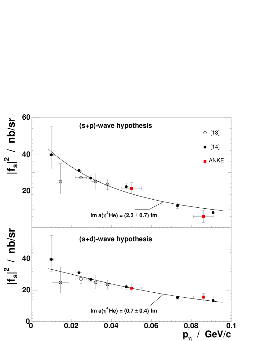
Figure 9: The square of the magnitude of the ${dd}\,\to\,^{4}\mathrm{He}\,\eta$ $s$–wave amplitude calculated with different assumptions concerning the partial wave decomposition, as discussed in the text. Upper panel: only $s$– and $p$–wave contributions. Lower panel: $s$– and $d$–wave contributions. The curves represent fits using the $s$–wave scattering length formula of eq. (4.2).

It is not possible from a single distribution such as that in fig. 9 to determine two real parameters; the error bars become strongly correlated. The authors of ref. Willis97 did a combined optical model fit to all the near–threshold ${pd}\,\to\,^{3}\mathrm{He}\,\eta$ and ${dd}\,\to\,^{4}\mathrm{He}\,\eta$ data, assuming that only $s$–wave production occurs, and this resulted in a value $a_{\eta\alpha}=(-2.2+1.1i)\>$fm. In this analysis the real part of $a_{\eta\alpha}$ was fixed mainly by the $\eta\,^{3}\mathrm{He}$ data and so the scattering length fits of fig. 9 have been carried out by varying just $\textrm{Im}(a_{\eta\alpha})$. This resulted in $a_{\eta\alpha}=(-2.2+2.3i)\>$fm and $(-2.2+0.7i)\>$fm respectively for the $s+p$ and $s+d$ assumptions. One can only attempt to separate these solutions by having measurements with a polarised beam, where eq. (A.8) allows $|C|^{2}$ to be extracted directly, e.g., from $t_{22}$.

5 Conclusions

By measuring the angular distribution of the ${dd}\,\to\,^{4}\mathrm{He}\,\eta$ reaction at two different energies, we have shown that higher partial waves affect the differential cross section at lower values of excess energy than for the corresponding ${pd}\,\to\,^{3}\mathrm{He}\,\eta$ reaction. The total cross sections link well with the results of previous measurements, though there is some ambiguity at the higher energies where the earlier data were taken with a polarised deuteron beam of helicity $m=\pm 1$. The uncertainty in the origin of the higher partial waves is reflected in the estimation of the $\eta\,\alpha$ scattering length from the data. Fixing the position of the pole in the $\eta\,\alpha$ scattering amplitude, which determines whether or not there is a quasi-bound state, requires an even more extensive data set, including especially more measurements with a polarised deuteron beam mariola , as well as data from below the $\eta\alpha$ threshold analogous to the studies for the $\eta^{3}$He system described in ref. Pfeiffer .

The only theoretical model designed to describe the ${dd}\,\to\,^{4}\mathrm{He}\,\eta$ reaction in a two–step approach has only been evaluated in the $s$-wave limit Faldt96 . It would be helpful to extend such calculations to higher waves to provide an indication as to which of these first becomes significant.

Appendix A ppendix: The ${dd\to\alpha\eta}$ amplitudes

In order to be able to isolate the $s$–wave amplitude from data on the production of pseudoscalar mesons in reactions such as $dd\to\alpha\eta$ or $dd\to\alpha\pi^{0}$, one has to make measurements of deuteron analysing powers as well as the differential cross section. The resulting analysis requires an understanding of the relationship between the amplitude structure and the observables, which is summarised in this appendix.

Due to the identical nature of the incident deuterons, only three independent scalar amplitudes are necessary to describe the spin dependence of the reaction. If we let the incident deuteron cms momentum be ${p}$ and that of the $\eta$ be ${p_{\eta}}$, then one choice for the structure of the transition matrix $\mathcal{M}$ is:

$$M = A({\mbox{\boldmath${\epsilon}$}}_{1}\times{\mbox{\boldmath${\epsilon}$}}_{2})\cdot\hat{\mbox{\boldmath${p}$}}+B({\mbox{\boldmath${\epsilon}$}}_{1}\times{\mbox{\boldmath${\epsilon}$}}_{2})\cdot\left[\hat{\mbox{\boldmath${p}$}}\times({\mbox{\boldmath${p}$}_{\eta}}\times\hat{\mbox{\boldmath${p}$}})\right]({\mbox{\boldmath${p_{\eta}}$}}\cdot{\hat{\mbox{\boldmath${p}$}}})$$ (A.1)

$$+C\left[({\mbox{\boldmath${\epsilon}$}}_{1}\cdot{\hat{\mbox{\boldmath${p}$}}}){\mbox{\boldmath${\epsilon}$}}_{2}\!\cdot\!({\mbox{\boldmath${p}$}_{\eta}}\times\hat{\mbox{\boldmath${p}$}})+({\mbox{\boldmath${\epsilon}$}}_{2}\cdot{\hat{\mbox{\boldmath${p}$}}}){\mbox{\boldmath${\epsilon}$}}_{1}\!\cdot\!({\mbox{\boldmath${p}$}_{\eta}}\times\hat{\mbox{\boldmath${p}$}})\right],$$

where the ${\mbox{\boldmath${\epsilon}$}}_{i}$ are the polarisation vectors of the two deuterons. Note that $\mathcal{M}$, which is a pseudoscalar due to the $\eta$ parity, is invariant under the transformation ${\mbox{\boldmath${\epsilon}$}}_{1}\rightleftharpoons{\mbox{\boldmath${\epsilon}$}}_{2}$, ${\mbox{\boldmath${p}$}}\to-{\mbox{\boldmath${p}$}}$, as required by Bose symmetry. The scalar amplitudes $A$, $B$, and $C$ are functions of ${\mbox{\boldmath${p}$}_{\eta}}^{2}$, ${\mbox{\boldmath${p}$}}^{2}$, and $({\mbox{\boldmath${p}$}_{\eta}}\cdot{\mbox{\boldmath${p}$}})^{2}=p_{\eta}^{2}p^{2}\cos^{2}\theta$, where $\theta$ is production angle of the $\eta$ meson.

Following the usual convention of letting ${p}$ lie along the $z$–direction and ${\mbox{\boldmath${p}$}_{\eta}}$ to be in the $x$–$z$ plane, the transition matrix reduces to:

$$\mathcal{M} = A\left[\epsilon_{1x}\epsilon_{2y}-\epsilon_{1y}\epsilon_{2x}\right]+Bp_{\eta}^{2}\sin\theta\cos\theta\left[\epsilon_{1y}\epsilon_{2z}-\epsilon_{1z}\epsilon_{2y}\right]$$ (A.2)

$$-Cp_{\eta}\sin\theta\left[\epsilon_{1z}\epsilon_{2y}+\epsilon_{1y}\epsilon_{2z}\right].$$

If we assume that deuteron–2 is unpolarised, the remaining polarisation information is contained within the density matrix:

$$\mathcal{Z}=\sum_{m_{2}}\mathcal{M}^{\dagger}\mathcal{M}\,.$$ (A.3)

Using the explicit form of eq. (A.2), and working in the spherical basis, the unpolarised intensity ($I$) and the vector ($t_{1i}$) and tensor ($t_{2i}$) analysing powers are obtained by taking the trace of $\mathcal{Z}$ with the unit matrix, and the vector and tensor projection operators $\Omega_{1i}$ and $\Omega_{2i}$ Hamilton . This leads to the expressions:

$$I = \mbox{${\textstyle\frac{2}{3}}$}\left(|A|^{2}+|B|^{2}p_{\eta}^{4}\sin^{2}\theta\cos^{2}\theta+|C|^{2}p_{\eta}^{2}\sin^{2}\theta\right),$$

$$I\,t_{20} = \mbox{${\textstyle\frac{1}{3\sqrt{2}}}$}\left(2|A|^{2}-|B|^{2}p_{\eta}^{4}\sin^{2}\theta\cos^{2}\theta\right.$$

$$\left.-|C|^{2}p_{\eta}^{2}\sin^{2}\theta-6\,\textrm{Re}\{B^{*}C\}p_{\eta}^{3}\sin^{2}\theta\cos\theta\right),$$

$$I\,t_{21} = -\mbox{${\textstyle\frac{1}{\sqrt{3}}}$}\,\textrm{Re}\left\{A^{*}(Bp_{\eta}\cos\theta+C)\right\}p_{\eta}\sin\theta,$$

$$I\,t_{22} = \mbox{${\textstyle\frac{1}{2\sqrt{3}}}$}\,|Bp_{\eta}\cos\theta-C|^{2}p_{\eta}^{2}\sin^{2}\theta,$$

$$I\,it_{11} = \mbox{${\textstyle\frac{1}{\sqrt{3}}}$}\,\textrm{Im}\left\{A^{*}(Bp_{\eta}\cos\theta+C)\right\}p_{\eta}\sin\theta,$$

$$I\,t_{10} = 0\,.$$ (A.4)

The term proportional to $C$ is the only one that changes sign under $\vec{p_{\eta}}\to-\vec{p_{\eta}}$ and thus represents odd $\eta\,\alpha$ partial waves; the other amplitudes correspond to even waves. Of these, the sole term that survives at threshold, and which therefore contains the $\eta\,\alpha$ $s$–wave, is proportional to $A$ so that the tensor analysing power $t_{20}=+1/\sqrt{2}$ at threshold and inspection of eq. (A.4) shows this to be true more generally at $\theta=0$.

For simplicity of presentation, we have adopted a notation in eq. (4.1) whereby the unpolarised differential cross section is related to the amplitudes by

$$\frac{\mbox{\rm d}\sigma}{\mbox{\rm d}\Omega}=\frac{p_{\eta}}{p}\,I\>.$$ (A.5)

The azimuthally symmetric differential cross sections for defined initial polarisation used in eq. (4.1) depend only then on $t_{20}$ and the unpolarised cross section through

$$\left(\frac{\mbox{\rm d}\sigma}{\mbox{\rm d}\Omega}\right)_{\!\!m=\pm 1} = \left(1+t_{20}/\sqrt{2}\right)\,\left(\frac{\mbox{\rm d}\sigma}{\mbox{\rm d}\Omega}\right),$$

$$\left(\frac{\mbox{\rm d}\sigma}{\mbox{\rm d}\Omega}\right)_{\!\!m=\pm 0} = \left(1-\sqrt{2}\,t_{20}\right)\,\left(\frac{\mbox{\rm d}\sigma}{\mbox{\rm d}\Omega}\right).$$ (A.6)

Since for our experimental data we are interested in describing the first deviations from an $s$-wave behaviour, we shall only keep terms that contribute to the observables up to order $p_{\eta}^{2}$. Though to this order $B$ and $C$ can be taken as constant at their threshold values, there can be an angular dependence in the $A$ amplitude which, to this order, may be written as the truncated Legendre expansion:

$$A=A_{0}+A_{2}\,p_{\eta}^{2}\,P_{2}(\cos\theta)\>.$$ (A.7)

To order $p_{\eta}^{2}$ therefore,

$$I = \mbox{${\textstyle\frac{2}{3}}$}\left(|A_{0}|^{2}+2\,p_{\eta}^{2}\textrm{Re}\{A_{0}^{*}A_{2}\}\,P_{2}(\cos\theta)\right.$$

$$\hskip 113.81102pt\left.+|C|^{2}p_{\eta}^{2}\sin^{2}\theta\right),$$

$$I\,t_{20} = \mbox{${\textstyle\frac{1}{3\sqrt{2}}}$}\left(2|A_{0}|^{2}+4\,p_{\eta}^{2}\textrm{Re}\{A_{0}^{*}A_{2}\}\,P_{2}(\cos\theta)\right.$$

$$\hskip 113.81102pt\left.-|C|^{2}p_{\eta}^{2}\sin^{2}\theta\right),$$

$$I\,t_{21} = -\mbox{${\textstyle\frac{1}{\sqrt{3}}}$}\,p_{\eta}\sin\theta\,\left[\textrm{Re}\{A_{0}^{*}B\}p_{\eta}\cos\theta+\textrm{Re}\{A_{0}^{*}C\}\right],$$

$$I\,t_{22} = \mbox{${\textstyle\frac{1}{2\sqrt{3}}}$}\,|C|^{2}p_{\eta}^{2}\sin^{2}\theta,$$

$$I\,it_{11} = \mbox{${\textstyle\frac{1}{\sqrt{3}}}$}\,p_{\eta}\sin\theta\,\left[\textrm{Im}\{A_{0}^{*}B\}p_{\eta}\cos\theta+\textrm{Im}\{A_{0}^{*}C\}\right],$$

$$I\,t_{10} = 0\,,$$ (A.8)

where the $s$–wave amplitude $A_{0}$ will have an additional $p_{\eta}$ dependence arising from the $\eta$-$\alpha$ final state interaction.

Thus measurements of the angular distributions of the unpolarised cross section, $t_{20}$, and $it_{11}$, would allow one to extract the values of $|A_{0}|^{2}$, Re$(A_{0}^{*}A_{2})$, $|C|^{2}$, Im$(A_{0}^{*}B)$, and Im$(A_{0}^{*}C)$. This would then lead to two two–fold ambiguities that could only be resolved by the measurement of $t_{21}$. To this order in the momentum expansion, the $t_{22}$ information is not independent, though it would provide some check on the systematics arising for example from the background subtraction and/or on the convergence of the momentum expansion.

References

- (1) L.C. Liu and Q. Haider, Phys. Rev. C 34 (1986) 1845.
- (2) Q. Haider and L.C. Liu, Phys. Lett. B 172 (1986) 257.
- (3) H.C. Chiang, E. Oset and L.C. Liu, Phys. Rev. C 44 (1991) 738.
- (4) R. Chrien et al., Phys. Rev. Lett. 60 (1988) 2595.
-
(5)
B.J. Lieb et al., COSY proposal 50 (2000):
www.fz-juelich.de/ikp/gem/Proposals/eta2000.ps - (6) C. Wilkin, Phys. Rev. C 47 (1993) 938.
- (7) S. Wycech, A.M. Green and J.A. Niskanen, Phys. Rev. C 52 (1995) 544.
- (8) A. Fix and H. Arenhövel, Phys. Rev. C 66 (2002) 024002.
- (9) S.A. Rakityansky et al., Few Body Syst. Suppl. 9 (1995) 227.
- (10) S.A. Rakityansky et al., Phys. Rev. C 53 (1996) 2043.
- (11) J. Berger et al., Phys. Rev. Lett. 61 (1988) 919.
- (12) B. Mayer et al., Phys. Rev. C 53 (1996) 2068.
- (13) R. Frascaria et al., Phys. Rev. C 50 (1994) 537.
- (14) N. Willis et al., Phys. Lett. B 406 (1997) 14.
- (15) M. Betigeri et al., Phys. Lett. B 472 (2000) 267.
- (16) R. Bilger et al., Phys. Rev. C 65 (2002) 044608.
- (17) H.H. Adam et al., Int. J. Mod. Phys. A 20 (2005) 643.
- (18) V.A. Tryasuchev, Phys. Atom. Nucl. 60 (1997) 186.
- (19) M. Pfeiffer et al., Phys. Rev. Lett. 92 (2004) 252001; 94 (2005) 049102.
- (20) C. Hanhart, Phys. Rev. Lett. 94 (2005) 049101.
- (21) A. Wrońska, PhD thesis, Jagiellonian University, Cracow (2005).
- (22) S. Barsov et al., Nucl. Inst. Meth. A 462 (2001) 364.
- (23) M. Abdel-Bary et al., Phys. Lett. B 619 (2005) 281.
- (24) H. Dombrowski et al., Nucl. Inst. Meth. A 386 (1997) 228.
- (25) J. Banaigs et al., Nucl. Phys. B 105 (1976) 52.
- (26) A. Abashian, N.E. Booth, and K.M. Crowe, Phys. Rev. Lett. 5 (1960) 258.
- (27) A. Gårdestig, G. Fäldt, and C. Wilkin, Phys. Rev. C 59 (1999) 2608.
- (28) F. Hibou et al., Phys. Rev. Lett. 83 (1999) 492.
-
(29)
GEANT3, CERN Program Library W5013 (1993):
www.cern.ch/wwwasdoc/geant html3/geantall.html - (30) G. Bizard et al., Phys. Rev. C 22 (1980) 1632.
- (31) M. Goldberger and K. Watson, Collision Theory (J. Wiley, New York, 1964).
-
(32)
H. Machner et al., COSY proposal 124 (2003):
www.fz-juelich.de/ikp/gem/Proposals/dd2alphaeta.pdf - (33) G. Fäldt and C. Wilkin, Nucl. Phys. A596 (1996) 488.
- (34) C. Hanhart, Phys. Rept. 397 (2004) 155.
- (35) J. Hamilton, The Theory of Elementary Particles, (OUP, Oxford, 1959).
- (36) The ANKE collaboration: www.fz-juelich.de/ikp/anke