The role of elliptic flow correlations in the discovery of the sQGP at RHIC

Abstract

Flow measurements are reviewed with particular emphasis on the hydrodynamic character of elliptic flow at RHIC. Hydrodynamic scaling compatible with the production of highly thermalized matter having a high degree of collective interactions and extremely low viscosity, is observed for a broad selection of the data. These properties suggest the production of a new state of strongly interacting nuclear matter at extremely high density and temperature where the relevant degrees of freedom are the valence quarks, ie. the sQGP.

1 Prologue

For more than twenty five years the heavy ion community has sought to create and study the quark gluon plasma (QGP) – a new phase of hot and dense nuclear matter where quarks and gluons are no longer confined to the interior of single hadrons. Such a state is predicted to exist at high energy densities by quantum chromodynamics (QCD) and is now very strongly indicated by lattice QCD calculations [1, 2]. The fundamental value of this search is rooted in the fact that the QGP; (i) is the ultimate primordial form of QCD matter at high temperature or baryon number density, (ii) was present during the first few microseconds of the Big Bang, (iii) provides an example of phase transitions which may occur at a variety of higher temperature scales in the early universe, and (iv) can provide important insights on the origin of mass for matter, and how quarks are confined into hadrons [3].

The use of flow correlations as a probe for the nuclear equation of state (EOS) and a possible phase transition, was recognized quite early [4, 5, 6, 7]. The connection is made transparent in the framework of perfect fluid dynamics where the conceptual link between the conservation laws (baryon number, and energy and momentum currents) and the fundamental properties of a fluid (its equation of state and transport coefficients) is straightforward. It is therefore not surprising that hydrodynamic considerations have played, and continue to play an important role in flow studies [8]. Fig. 2 shows the result of an early fluid-dynamical calculation which illustrates the development of flow correlations in Ne+U collisions. Fig. 2 shows a schematic diagram of a more recent conjecture that jet interaction with a high energy density medium could lead to the generation of a Mach cone and hence conical flow [9].

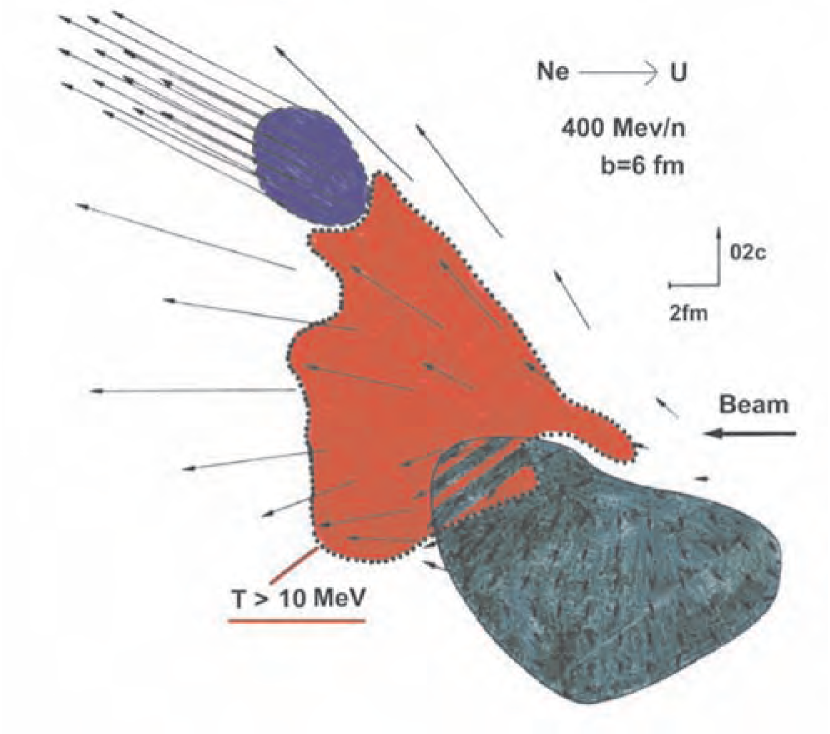
Figure 1: Density and temperature contours in the scattering plane of a mid-central Ne+U collision. The arrows indicate velocity fields. Results are from a fluid-dynamical calculation [7].

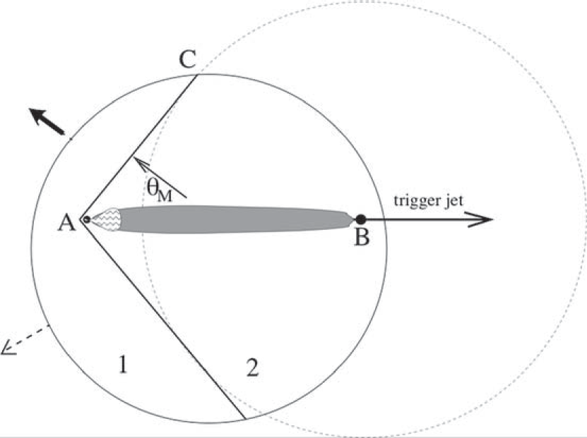
Figure 2: Schematic diagram of the development of a Mach cone resulting from the strong interaction between a jet and a high energy density medium [9]. The arrows which point to the left indicate the direction of flow normal to the shock cone.

1.1 Azimuthal distributions and flow correlations

Azimuthal angle distributions and correlation functions play a pivotal role in the study of flow correlations. Experimentally, one measures the magnitude of flow correlations by evaluating the Fourier coefficients $\lambda_{n}$, of the anisotropy of the distribution in azimuthal angle difference ($\Delta\phi=\phi_{1}-\phi_{2}$) between pairs of charged hadrons [10, 11, 12]

$$\frac{dN}{d\Delta\phi}\propto\sum\limits_{n=-\infty}^{\infty}{\lambda_{n}}e^{in\Delta\phi},\ \hskip 14.22636pt\lambda_{n}=\langle e^{in\Delta\phi}\rangle.$$ (1)

Here $\phi_{1,2}$ are the azimuthal angles of a pair of particles measured in the laboratory coordinate system, and the brackets denote an average over pairs of particles emitted in an event followed by further averaging over events. Alternatively, the Fourier coefficients $v_{n}$ can be obtained as [13, 14, 15, 16]:

$$v_{n}\equiv\langle e^{in(\phi-\Phi_{R})}\rangle=\langle\cos n(\phi-\Phi_{R})\rangle,$$ (2)

where $\phi$ is the azimuthal angle of an emitted particle (also measured in the laboratory coordinate system) and $\Phi_{R}$ is an estimate of the azimuth of the reaction plane. A requisite correction which takes account of the dispersion of the reaction plane is easy to evaluate [13, 14, 15, 16].

For detectors having a limited $\phi$ acceptance, the correlation function $C_{2}(\Delta\phi)$, is often exploited to measure $\lambda_{n}$ [10, 11, 12]:

$$C_{2}\left({\Delta\phi}\right)=\frac{{N_{cor}\left({\Delta\phi}\right)}}{{N_{mix}\left({\Delta\phi}\right)}}=\sum\limits_{-\infty}^{+\infty}{\lambda_{n}e^{in\Delta\phi}},$$ (3)

where the correlated distribution $N_{cor}\left({\Delta\phi}\right)$, is obtained from pair members belonging to the same event. The mixed distribution $N_{mix}\left({\Delta\phi}\right)$, is made of pair members belonging to different events having characteristics (multiplicity, vertex, etc.) similar to those for $N_{cor}\left({\Delta\phi}\right)$. The correlation between each particle and the reaction plane induces correlations among all particles. Thus, it is straightforward to show that $\lambda_{n}=v_{n}^{2}$ when both particles are selected from the same $p_{T}$ and rapidity $y$, range (ie. fixed-$p_{T}$ correlations) and $\lambda_{n}=v_{n}(1)v_{n}(2)$ when particle (1) and (2) are selected from a different $p_{T}$ and/or y range (ie. assorted correlations). When $v_{n}$ is measured for specific particle species or as a function of transverse momentum, centrality and/or rapidity, they are referred to as “differential” flow measurements. When the measurements are averaged over a sizable phase space they are termed “integral” measurements. The first two coefficients, $v_{1}$ and $v_{2}$, are usually referred to as directed flow and elliptic flow, respectively.

In addition to the consideration of detector acceptance, reliable flow measurements often require the suppression of so called non-flow correlations. These include small-angle correlations due to final state interactions and quantum statistical effects [17], correlations due to resonance decays [18] and mini-jet production [19]. The methods of Lee Yang zeros [20] and cumulants [21] have been developed to suppress such non-flow correlations. The cumulant method is based on a cumulant expansion of multi-particle correlations [21]. The method of Lee Yang zeros follows the spirit of the Lee Yang theory of phase transitions [22], and extracts flow directly from the genuine correlations involving a large number of particles [20].

Azimuthal distributions are not only important for flow measurements. They are of great current interest in connection with the study of jet modification [23], the formation of disoriented chiral condensates [24, 25], and the study of parity and/or time-reversal violation[26]. The combined use of flow correlations and two-particle interferometry measurements is also used extensively to gain detailed insight on the three-dimensional structure of emitting sources [27, 28, 29].

1.2 A snapshot of over twenty years of elliptic flow measurements

Systematic flow measurements now exist for a beam energy range which spans nearly six orders of magnitude. They include measurements done at MSU, GANIL, BEVALAC, GSI, Dubna, AGS, SPS and RHIC. Results for elliptic and directed flow in Au+Au collisions, from several of these measurements are summarized in Figs. 4 and 4 respectively.

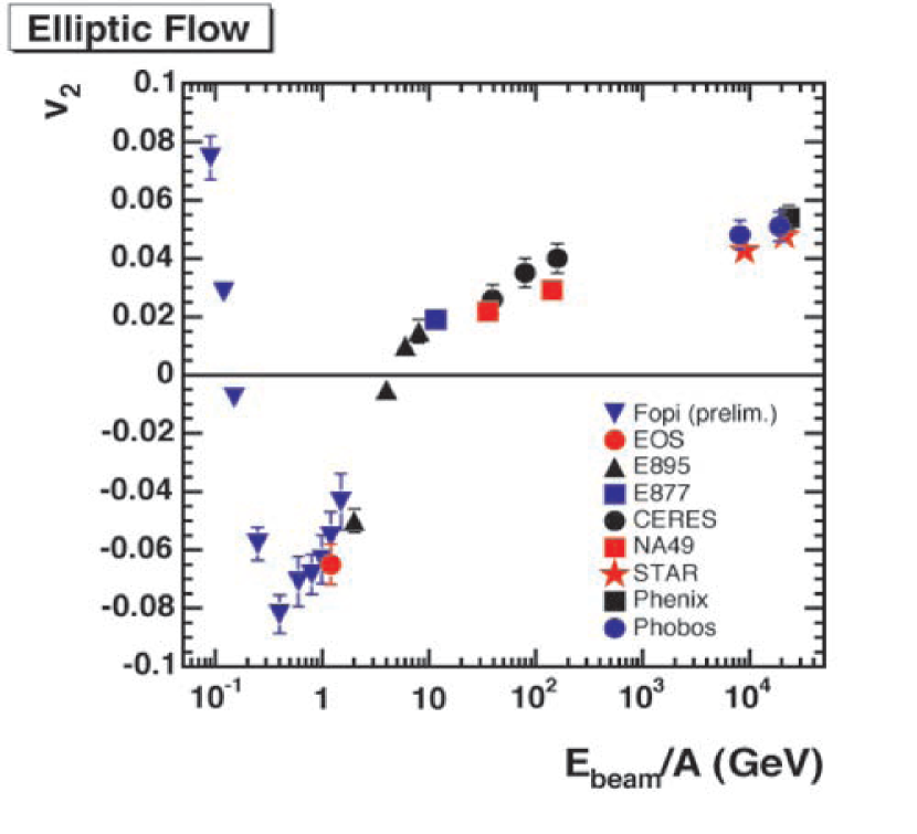
Figure 3: Elliptic flow ($v_{2}$) vs beam energy for mid-central collisions Au+Au colllisions [34].

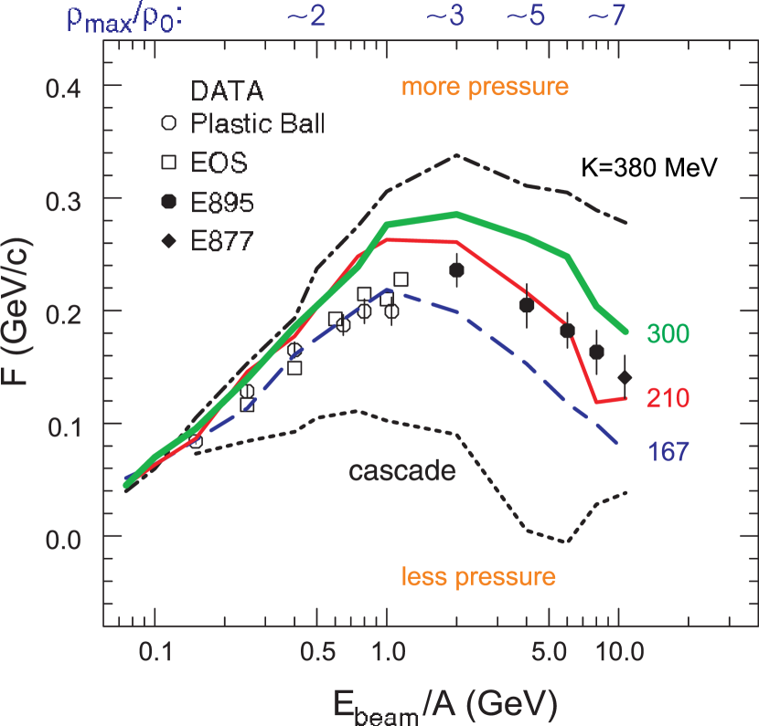
Figure 4: Directed flow vs. beam energy for mid-central Au+Au collisions. The lines show transport theory predictions for different EOS’s [35].

For a broad range of beam energies ($E_{beam}/A\geq$ 400 MeV), the elliptic flow results can be understood in terms of a delicate balance between (i) the ability of pressure developed early in the reaction zone, to effect a rapid transverse expansion of nuclear matter, and (ii) the passage time for removal of the shadowing of participant hadrons by the projectile and target spectators[32, 33, 35]. The characteristic time for the development of expansion perpendicular to the reaction plane is $\sim R/c_{s}$, where the speed of sound $c_{s}=\sqrt{\partial P/\partial\varepsilon}$, $R$ is the nuclear radius, $P$ is the pressure and $\varepsilon$ is the energy density. The passage time is $\sim 2R/\left({\gamma_{0}v_{0}}\right)$, where $v_{0}$ is the c.m. spectator velocity.

If the passage time is long compared to the expansion time, spectator nucleons serve to block the path of participant hadrons emitted toward the reaction plane, and nuclear matter is squeezed-out perpendicular to this plane giving rise to negative elliptic flow. The squeeze-out contribution should then reflect the ratio $c_{s}/\left({\gamma_{0}v_{0}}\right)$. This is put into evidence in Fig. 6 where the differential elliptic flow values $v_{2}(p_{T})$, shown for beam energies of 0.4 - 2 AGeV in Fig. 6, are scaled by the passing time. The rather good scaling observed suggest that $c_{s}$ does not change significantly over this beam energy range.

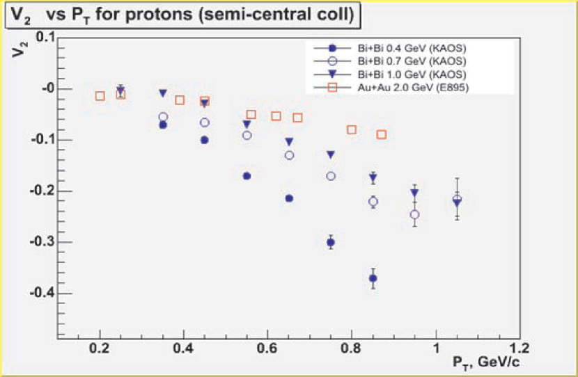
Figure 5: Differential flow $v_{2}(p_{T})$ vs $p_{T}$ for several beam energies. The data are from Refs. [36, 37]

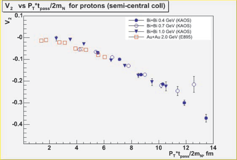
Figure 6: The same data shown in Fig. 6 scaled by the passing time.

For very short passage times (such as those at top AGS energies and beyond), the inertial confinement of participant matter is significantly reduced and preferential in-plane emission or positive elliptic flow is favored. This is so because the geometry of the participant region exposes a larger surface area in the direction of the reaction plane and pressure gradients in this direction are also larger. Thus, the observed trends ( ie. negative for beam energies $<4$ AGeV and positive for beam energies $>4$ AGeV) for the beam energy dependence of elliptic flow are well understood [32, 33, 37]. For RHIC energies, strong Lorentz contraction and very short passage times lead to significant reduction of shadowing effects, and positive elliptic flow is driven primarily by the anisotropies in the transverse pressure gradients [38, 39, 40].

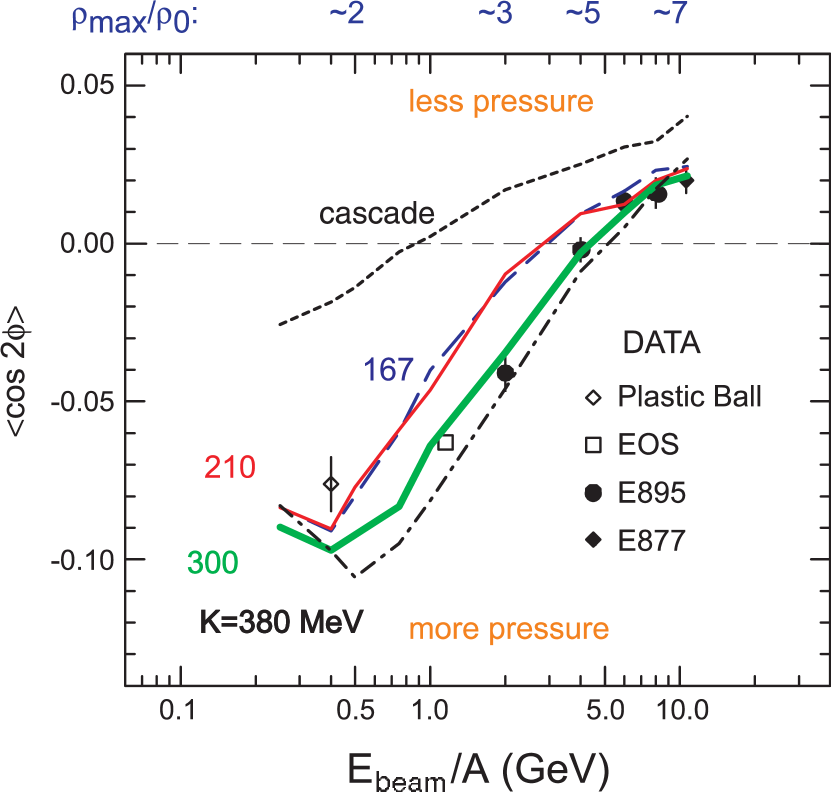
Figure 7: Differential flow $v_{2}$ vs $E_{beam}$ for the energy range 0.4 $<E_{beam}<$ 12.0 AGeV. Results are shown for protons for mid-central collisions [35].

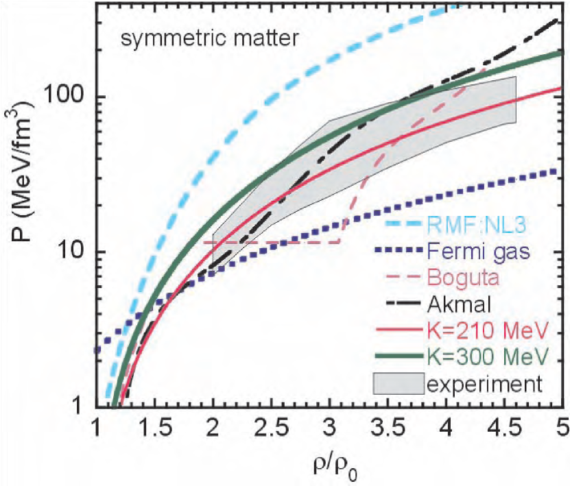
Figure 8: Zero temperature EOS. The shaded region is the region of pressures consistent with the experimental flow data. The curves show predictions for different EOS’s [35].

1.3 Pre-RHIC constraints for the EOS

The elliptic and directed flow observables are sensitive to the mean field and to the equation of state. Consequently, comparisons of these two observables to model calculations can provide important constraints for the EOS. Such comparisons have been carried out for the beam energy range 0.4 $<E_{beam}<$ 12.0 AGeV [35].

Figs. 4 and 8 show comparisons for several incompressibility constants ($K$). At incident energies of 2-6 GeV/A, for example, the transverse flow data lie near or somewhat below (to the low pressure side of) the $K=210$ MeV calculations, while the elliptic flow data lie closer to the $K=300$ MeV calculations. The calculations without a mean field (cascade) or with a weakly repulsive mean field ($K=167$ MeV) provide too little pressure to reproduce either flow observable at higher incident energies (and correspondingly higher densities). The calculations with $K=167$ MeV and K=380 MeV provide lower and upper bounds on the pressure in the density range $2.0<\rho/\rho_{0}<5.0$.

If one factors in the uncertainties due to the momentum dependencies of the mean fields and the collision integral, a range of pressure-density relationships can be established from the comparisons made in Figs. 4 and 8. These bounds on the equation of state are shown for zero temperature matter by the shaded region in Fig. 8. They constitute the most current set of constraints on the EOS for high energy density nuclear matter created at high baryon densities, and can provide a rudimentary base-line for comparisons involving the essentially baryon-free matter created at RHIC.

2 Elliptic flow at RHIC

2.1 The nature of the “soft” matter formed at RHIC

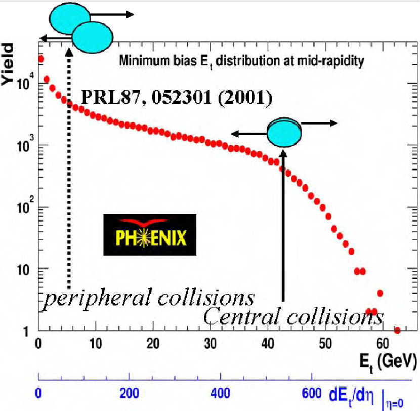
Figure 9: Yield vs transverse energy $E_{t}$. The data are obtained from Ref. [44].

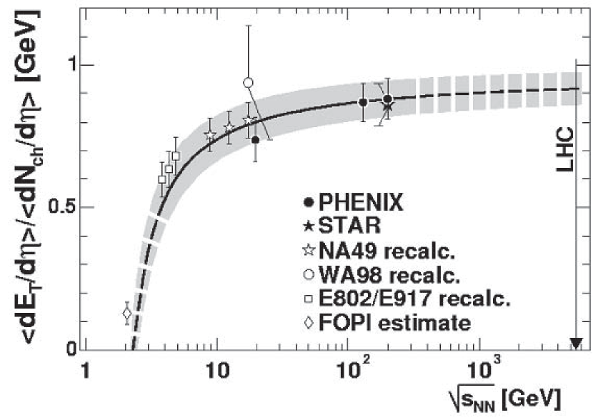
Figure 10: $\left\langle E_{T}\right\rangle/\left\langle N_{ch}\right\rangle$ vs. $\sqrt{s_{NN}}$ for Au+Au collisions. The data are taken from Ref. [45].

It is a well known fact that rather high energy densities are achieved in central and semi-central heavy ion collisions at RHIC [44, 46]. Fig. 10 shows a recent measurement of the transverse energy $E_{T}$, distribution for central Au+Au collisions at $\sqrt{s_{NN}}=130$ GeV. Following the commonly exploited Bjorken ansatz

$$\varepsilon_{Bj}=\frac{1}{{\pi\,R^{2}}}\;\frac{1}{{\tau_{0}}}\;\frac{{dE_{T}}}{{dy}},$$

if we assume a thermalization time $\tau_{0}\sim 0.2-1$ fm/c, one obtains the energy density $\varepsilon_{Bj}=5~{}-~{}15$ GeV/fm³, which is 35 - 100 times the energy density $\varepsilon_{0}$, for normal nuclear matter. This energy density far exceeds the lattice QCD estimate ($\sim 1$ GeV/fm³) for creating a de-confined phase of quarks and gluons (QGP)[1, 2]. Fig. 10 shows the $\sqrt{s_{NN}}$ dependence of the ratio $\left\langle E_{T}\right\rangle/\left\langle N_{ch}\right\rangle$, obtained for Au+Au collisions spanning the collision energy range SIS - RHIC. It shows that the $\left\langle E_{T}\right\rangle$ rises faster than the mean multiplicity for charge particle production $\left\langle N_{ch}\right\rangle$, from SIS to SPS energies. However, there is little change in the ratio $\left\langle E_{T}\right\rangle/\left\langle N_{ch}\right\rangle$ from SPS to RHIC, suggesting that the $\sqrt{s_{NN}}$ increase results primarily in an increase in particle production.

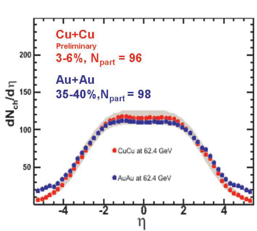
Figure 11: Comparison of the multiplicity distributions for Cu+Cu and Au+Au collisions obtained for the same number of participants at $\sqrt{s_{NN}}=62.4$ GeV. The data are obtained from Ref. [46].

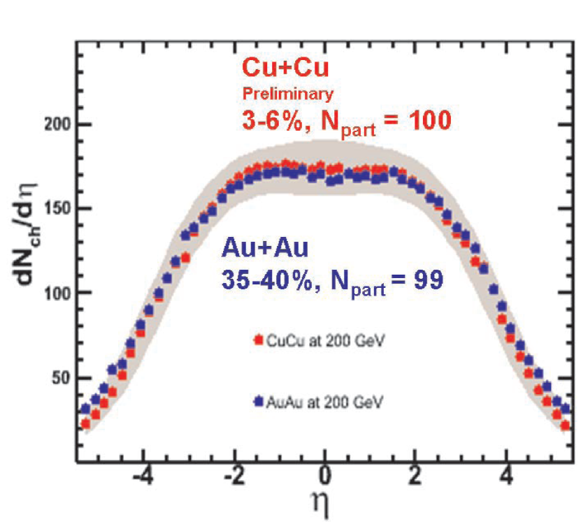
Figure 12: Comparison of the multiplicity distributions for Cu+Cu and Au+Au collisions obtained for the same number of participants at $\sqrt{s_{NN}}=200.0$ GeV. The data are obtained from Ref. [46].

There are strong hints that this particle production follows rapid thermalization. First, the multiplicity distribution for the same number of participants is independent of colliding system size, as would be expected from a system which “forgets” how it is formed. A beautiful demonstration of this is shown in Figs. 12 and 12 with PHOBOS data for Au+Au and Cu+Cu collisions at two separate collision energies.

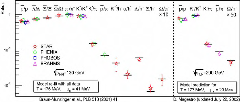
Figure 13: Comparison of measured particle ratios for Au+Au collisions, with the predictions of a statistical model (solid lines).

Second, a comparison of the measured anti-particle to particle ratios with the predictions of a statistical model

$$\frac{{\bar{p}}}{p}=\frac{{e^{-(E+\mu)/T}}}{{e^{-(E-\mu)/T}}}=e^{-2\mu/T},$$

gives excellent agreement as shown for Au+Au collisions in Fig. 13. It is noteworthy that the the temperature $T\sim 176$ MeV, required for this excellent agreement compares well with the critical temperature $T_{cr}\sim 170$ MeV, required for the QGP phase transition. The baryochemical potential $\mu$, extracted for this temperature, increases from $\sim 29$ MeV at $\sqrt{s_{NN}}=200.0$ GeV to $\sim 40$ MeV at $\sqrt{s_{NN}}=130.0$ GeV.

Given the large energy densities produced in RHIC collisions, if thermalization does indeed occur, then one expects the development of large pressures;

$${{P}=\rho\cdot\left.{\left({{\raise 3.01385pt\hbox{${\partial\varepsilon}$}\!\mathord{\left/{\vphantom{{\partial\varepsilon}{\partial\rho}}}\right.\kern-1.2pt}\!\lower 3.01385pt\hbox{${\partial\rho}$}}}\right)}\right|_{{{s/}}\rho}}.$$

More importantly, if thermalization is rapid in non-central collisions, then large pressure gradients resulting from the initial spatial anisotropy or eccentricity

$$\epsilon=\left({\left\langle{y^{2}}\right\rangle-\left\langle{x^{2}}\right\rangle}\right)/\left({\left\langle{y^{2}}\right\rangle+\left\langle{x^{2}}\right\rangle}\right),$$

of the collision zone would lead to strong elliptic flow. That is, the observation of large elliptic flow for a variety of particle species would be compatible with the expectation for early thermalization.

2.2 Elliptic flow results

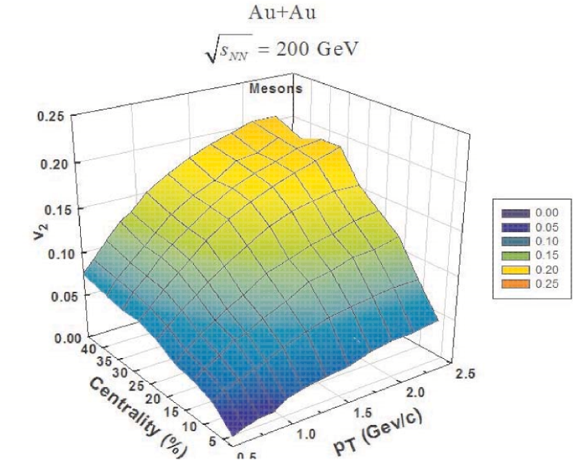
Figure 14: PHENIX preliminary data for the doubly differential anisotropy $v_{2}(centrality,p_{T})$, for mesons (dominantly pions).

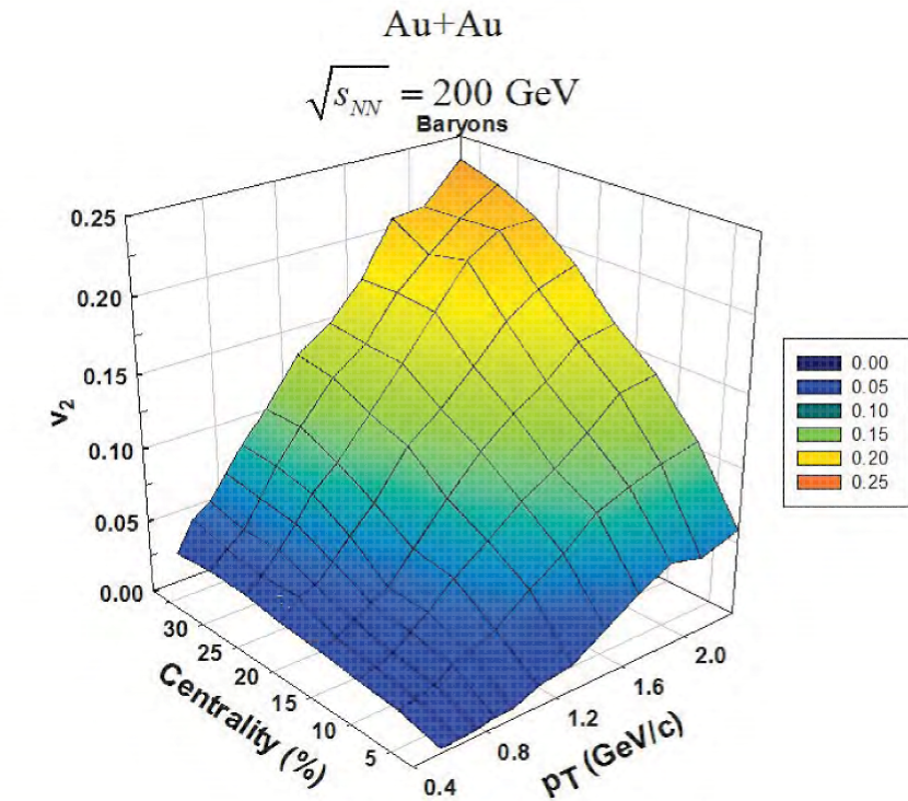
Figure 15: PHENIX preliminary data for the doubly differential anisotropy $v_{2}(centrality,p_{T})$, for protons and anti-protons.

Detailed differential and integral measurements are now available for charged hadrons and a variety identified particle species ($\mathrm{p},\pi,K,\Lambda,\Omega,\phi,\Xi,\mathrm{d},\mathrm{D}$) at RHIC [47]. Figs. 15 and 15 summarize the extracted doubly differential anisotropy $v_{2}(centrality,p_{T})$, for mesons (dominantly pions) and baryons (protons and anti-protons). They give an excellent overview of the the detailed evolution of $v_{2}$ as centrality and $p_{T}$ are varied. The results shown for protons ($p$) and anti-protons ($\overline{p}$) give an especially good view of the evolution away from the well known quadratic dependence of $v_{2}(p_{T})$ (which is also observed in very central collisions for these data) as the collisions become more peripheral.

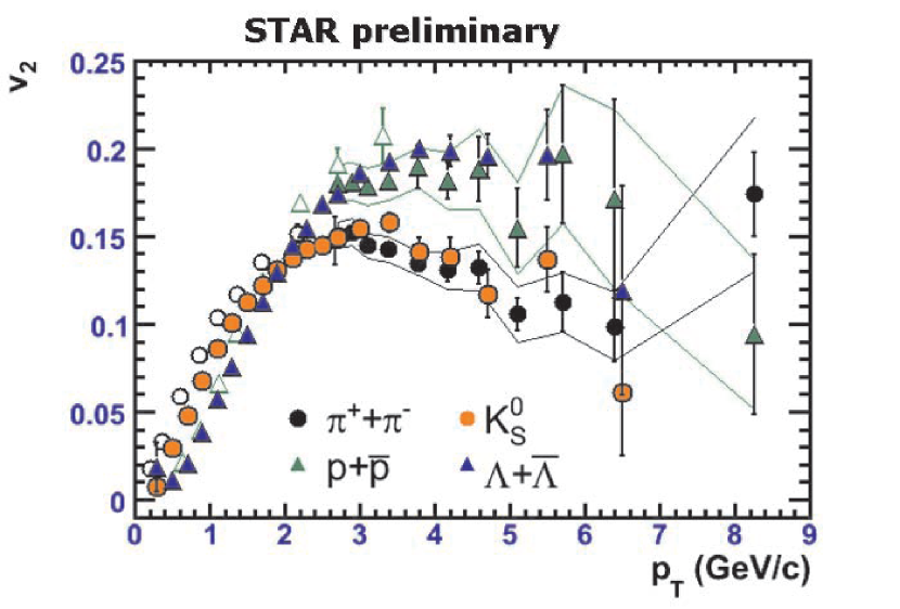
Figure 16: Preliminary STAR data showing $v_{2}(p_{T})$ vs. $p_{T}$ for different particle species produced in Au+Au collisions at $\sqrt{s_{NN}}=200$ GeV [47].

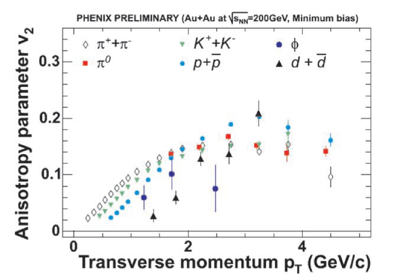
Figure 17: Preliminary PHENIX data showing $v_{2}(p_{T})$ vs. $p_{T}$ for different particle species produced in Au+Au collisions at $\sqrt{s_{NN}}=200$ GeV [47].

Figs. 17 and 17, show a representative set of differential flow measurements $v_{2}(p_{T})$ for several different particle species. They are all characterized by rather large magnitudes compatible with the predictions of the hydrodynamic model [39, 40, 41], which in turn implies the creation of a strongly interacting medium and essentially full local thermal equilibrium. It is especially noteworthy that the $v_{2}$ values for the $\phi$ are comparable to those of other hadrons. Given its rather small re-scattering cross section, such $v_{2}$ values suggest that thermalization is rapid and pressure gradients develop at the partonic level.

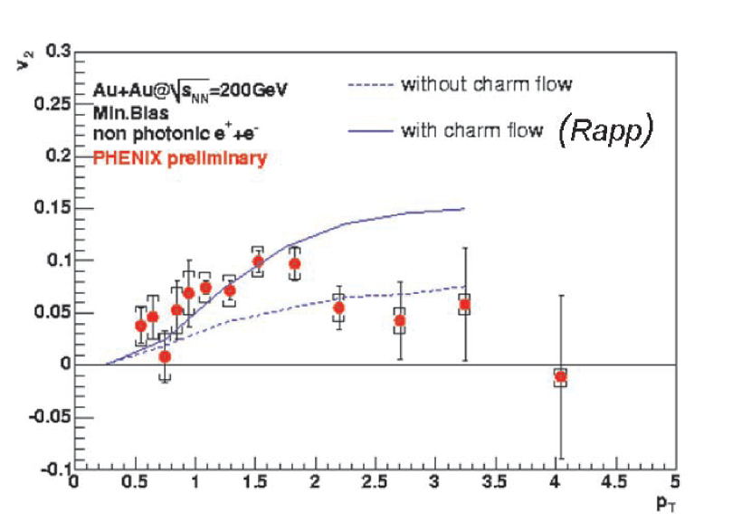
Figure 18: $v_{2}(p_{T})$ vs. $p_{T}$ for charm [42]. The lines compare the results from a calculation which includes/excludes charm flow [49].

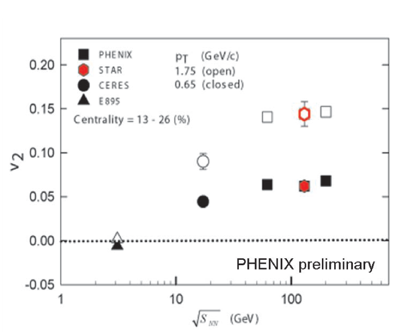
Figure 19: $\sqrt{s_{NN}}$ dependence of $v_{2}$ for fixed $p_{T}$ selections of 0.65 and 1.75 GeV/c from A+A collisions with A $\approx 200$ [50].

Further evidence for rapid thermalzation can also be found in the recent measurements of $v_{2}$ for non-photonic electrons [42]. Such measurements provide a probe for whether or not the charm quark flows. Fig. 19 compares recent PHENIX measurements to the calculations of Rapp et al. [49]. The good agreement (for $p_{T}<2$ GeV/c) between the data and the calculation which includes charm flow, suggests heavy quark thermalization in RHIC collisions.

As discussed earlier, the pressure or energy density gradients provide the fluid acceleration necessary to develop the large observed values of $v_{2}$. The initial energy density controls how much flow can develop globally, since it sets the overall time scale between the beginning of hydrodynamic expansion and final decoupling. On the other hand, the detailed development of the flow patterns are controlled by the temperature dependent speed of sound $c_{s}^{2}=\partial P/\partial\varepsilon$. Lattice QCD calculations indicate that $c_{s}^{2}\approx 1/3$ for $T>2T_{cr}$, but drops steeply by more than a factor of six near the “softest point” where $T\approx T_{cr}$. Thereafter, it rises again in the hadron resonance gas phase to the value $c_{s}^{2}\approx 0.15$. Given this, an important question is whether or not there might be a trace of this “softest point” in the data.

Fig. 19 shows the $\sqrt{s_{NN}}$ dependence of $v_{2}$ over a broad range of bombarding energies for two $p_{T}$ selections. The data show essentially no beam energy dependence over the entire energy range explored at RHIC, but decreases substantially as one moves down to the lower SPS and AGS energies. These data reflect the predicted non-monotonic structure in the elliptic flow excitation function [51]. However, they do not show the decrease (due to very strong softening of the EOS in the phase transition region) followed by a recovery in the moderately stiff hadron gas phase predicted by the model [51]. Nonetheless, the apparent saturation of $v_{2}$ above $\sqrt{s_{NN}}$ = 62.4 GeV does not exclude the role of a rather soft equation of state resulting from the production of a mixed phase [52] for the range $\sqrt{s_{NN}}$ = 62.4 - 200 GeV.

3 Universal scaling and perfect fluid hydrodynamics

A particularly important question of great current interest is whether or not the fine structure of azimuthal anisotropy (ie. its detailed dependence on centrality, transverse momentum, particle type, higher harmonics, etc) can provide valuable constraints on (i) the range of validity of perfect fluid hydrodynamics, (ii) the parameters of the model and (iii) the onset of competing mechanisms such as quark-coalescence [53]. One approach to address such questions, is the detailed investigation of flow data to test the validity and/or failure of several scaling “laws” predicted by perfect fluid hydrodynamics.

An important scaling prediction of hydrodynamic theory is exemplified by the exact analytic hydro solutions [54] exploited in the Buda-Lund model [55, 56]. The model gives:

$$v_{2n}=\frac{I_{n}(w)}{I_{0}(w)},n=1,2,..,{\mathrm{}}w=\frac{p_{t}^{2}}{4\overline{m}_{t}}\left(\frac{1}{T_{y}}-\frac{1}{T_{x}}\right),$$ (4)

where $I_{0,n}$ are modified Bessel-functions, $\overline{m}_{t}$ is a rapidity dependent average transverse mass (at midrapidity, $\overline{m_{T}}=m_{T}$, see ref. [56] for details), and $T_{x}$ and $T_{y}$ are direction ($x$ and $y$) dependent slope parameters:

$$T_{x} = T_{0}+\overline{m}_{t}\,\dot{X}_{f}^{2}\frac{T_{0}}{T_{0}+\overline{m}_{t}a},$$ (5)

$$T_{y} = T_{0}+\overline{m}_{t}\,\dot{Y}_{f}^{2}\frac{T_{0}}{T_{0}+\overline{m}_{t}a}.$$ (6)

Here, $\dot{X}_{f}$ and $\dot{Y}_{f}$ gives the transverse expansion rate of the fireball at freeze-out, and $a=(T_{0}-T_{s})/T_{s}$ is its transverse temperature inhomogeneity, characterized by the temperature at its center $T_{0}$, and at its surface $T_{s}$. The thermal and collective contributions can be made more transparent by replacing $p_{T}$ with the transverse rapidity $y_{T}=0.5\log((m_{T}+p_{T})/(m_{T}-p_{T}))$, to give the following approximate scaling law:

$$v_{2}\sim\frac{{k_{1}}}{{T_{0}}}\times y_{T}^{2}m\left({1+\frac{{k_{2}}}{{k_{1}}}\frac{{T_{0}}}{m}+\frac{{k_{3}}}{{k_{1}}}\left({\frac{{T_{0}}}{m}}\right)^{2}+..}\right),$$ (7)

where $k_{1,2,3}$ are mass ($m$) dependent constants. Equation 7 shows that $v_{2}$ should scale as $\sim k_{m}\times my_{T}^{2}$ for different particle species or flavor. Hereafter, we define the scaled variable $y^{fs}_{T}\equiv k_{m}\times my_{T}^{2}$. The higher harmonic $v_{4}\sim\frac{1}{2}v_{2}^{2}+k_{4}y_{T}^{4}$, can be similarly obtained from Eq. 4. It is also easy to show that $v_{2}$ scales with eccentricity and should be independent of the mass (size) of the colliding system for the same eccentricity. In what follows, we test whether or not such scaling is evidenced by RHIC data. The extent to which such scaling holds, gives an indication of the applicability and validity of perfect fluid hydrodynamics.

3.1 Eccentricity scaling & system size dependence

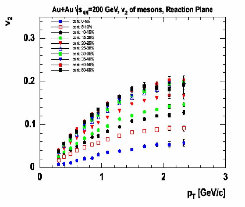
Figure 20: Doubly differential anisotropy $v_{2}(centrality,p_{T})$ vs. $p_{T}$. Preliminary PHENIX data are shown for several centrality selections for Au+Au collisions [47].

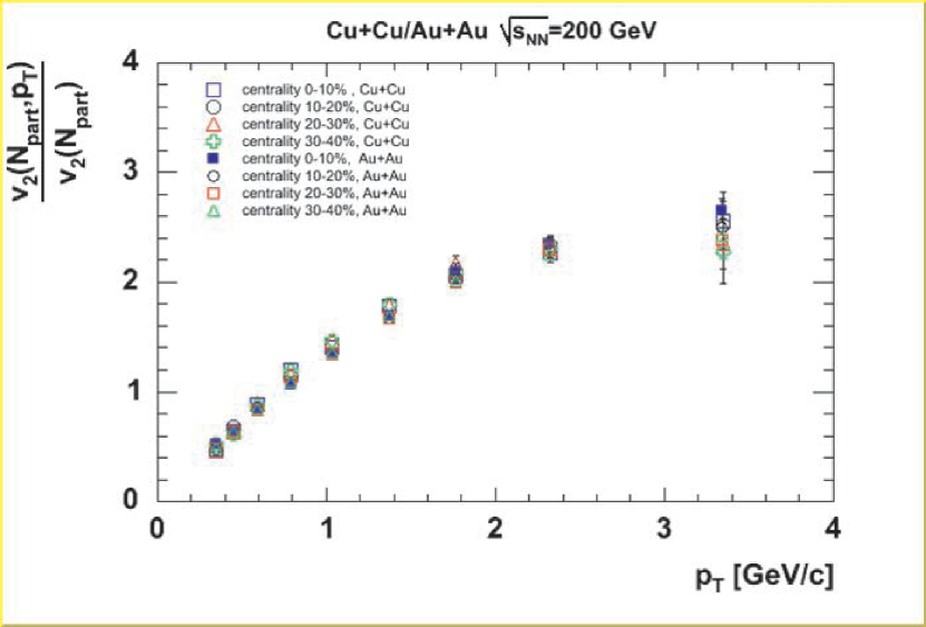
Figure 21: Scaled doubly differential anisotropy $v_{2}(centrality,p_{T})/v_{2}(centrality)$ vs. $p_{T}$. Preliminary PHENIX data are shown for several centrality selections for Au+Au and Cu+Cu collisions [47].

Fig. 21 show the differential $v_{2}(centrality,p_{T})$, for mesons for several centralities. It shows the very well known dependence of $v_{2}$ on $p_{T}$ and centrality. Fig. 21 show $v_{2}$ results for Cu+Cu and Au+Au scaled by the $p_{T}$-integrated $v_{2}$ value obtained for each centrality selection. We note here that the $p_{T}$-integrated flow is monotonic and linearly related to the eccentricity over a broad range of centralities. The scaled data for Au+Au and Cu+Cu shown in Fig. 21, are clearly compatible with the predicted eccentricity scaling. The fact that Cu+Cu and Au+Au scale to the same value indicates that the scaled $v_{2}$ values are independent of system size as predicted.

3.2 Particle flavor, pseudo-rapidity & higher harmonic scaling

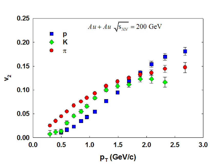
Figure 22: Differential anisotropy $v_{2}(p_{T})$ for protons, pions and kaons vs. $p_{T}$ [47].

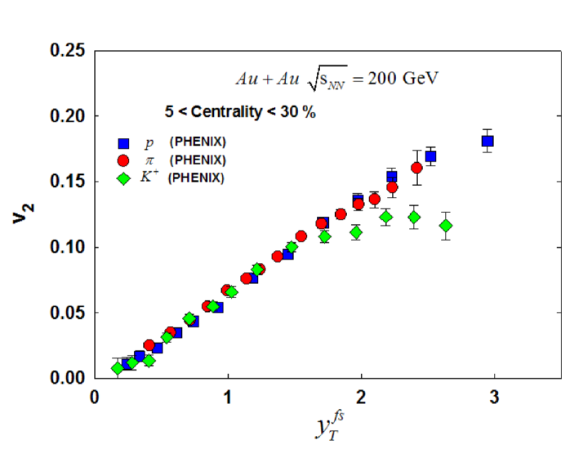
Figure 23: Differential anisotropy $v_{2}(y^{fs}_{T})$ for protons, pions and kaons vs. $y^{fs}_{T}$, see text.

Fig. 23 shows a comparison of the differential anisotropy $v_{2}(p_{T})$ for protons, kaons and pions obtained for the centrality selection 5-30%. The well known and rather characteristic flavor dependence of $v_{2}$ is clearly exhibited in the figure. If this aspect of the fine structure of $v_{2}$ has a hydrodynamic origin then the prediction is that it should scale with the variable $y^{fs}_{T}\equiv k_{m}\times my_{T}^{2}$. Fig. 23 shows $v_{2}$ data for the same particle species scaled by the fine structure scaling variable $y^{fs}_{T}$. The results indicate scaling over a relatively broad range in $y^{fs}_{T}$. It is interesting to note here that scaling appears to break in the $y^{fs}_{T}$ range where quark number scaling seem to work [53]. On the other hand, the latter is based on the coalescence of quarks which are flowing. Thus, hydrodynamic flow appears to dominate the dynamics for both low and intermediate $p_{T}$ particles.

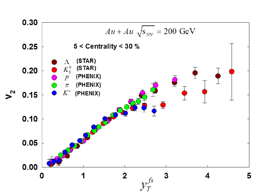
Figure 24: Differential anisotropy $v_{2}(y^{fs}_{T})$ vs. $y^{fs}_{T}$ for several different particles as indicated. The data are obtained from Refs. [47] and [48]

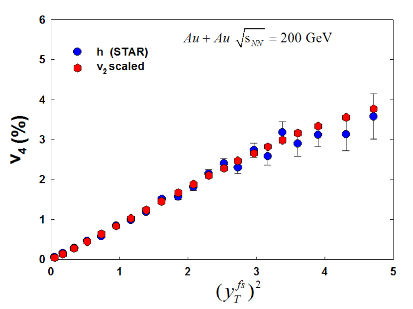
Figure 25: Comparison of measured and predicted $v_{4}$ for charged hadrons. The data are obtained from Ref. [48].

Fig. 25 shows $v_{2}$ data for a much larger selection of particle species (from both PHENIX and STAR) scaled by the fine structure scaling variable $y^{fs}_{T}$. Here again, the results indicate scaling over a relatively broad range in $y^{fs}_{T}$. The observed flavor scaling in these data provides rather strong evidence that the observed anisotropy is derived from a hydrodynamic origin. This conclusion is also supported by the good agreement obtained between the measured $v_{4}$ and the scaled values ($\acute{v_{4}}\sim\frac{1}{2}v_{2}^{2}+k_{m}y_{T}^{4}$) shown in Fig. 25.

An excitation function of the pseudo-rapidity dependence of $v_{2}$ also serves as an important test for the predictions of perfect fluid hydrodynamics. Fig. 27 shows results from a recent analysis of PHOBOS data [57]. The theoretical curves shown in the figure, give strong indications that these data are consistent with the analytic predictions of perfect fluid hydrodynamics  [55, 56].

3.3 Quark number scaling

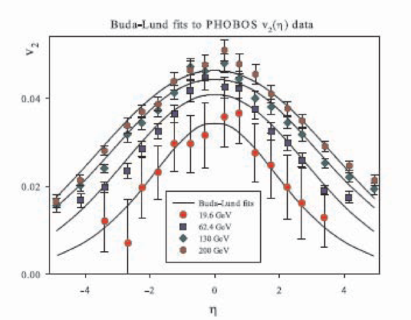
Figure 26: PHOBOS data showing $v_{2}$ vs. $\eta$. The curves show the results of theoretical calculations [57].

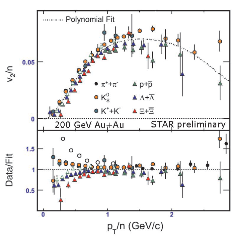
Figure 27: $v_{2}/n$ vs. $p_{T}/n$; $n$ is the number of valence quarks. The bottom panel show the deviations from quark number scaling [47].

The universal scaling discussed above, clearly speaks to the validity of perfect fluid hydrodynamics over a broad range of the observed data. However, such scaling does not provide explicit evidence for the degrees of freedom in the flowing matter. For intermediate values of $p_{T}$, hydrodynamic scaling breaks down (cf. Fig. 23) and the degrees of freedom can reveal themselves. Fig. 27 shows the results from a recent test for quark number scaling of $v_{2}$ by the STAR collaboration [47]. The lower panel of the figure illustrates the deviations from the quark coalescence ansatz used to scale the data shown in the top panel. The deviations are largest at low $p_{T}$ where hydrodynamic scaling was shown to work best. For intermediate $p_{T}$s (where the fluid dynamical picture breaks down) the deviations are quite small, suggesting that the active and relevant degrees of freedom are those of constituent or valence quarks.

4 Conical flow revisited

Objects moving at supersonic speeds create “conical flow” behind the shock front they create. Such flow were initially conjectured to occur in cold nuclear matter [58]. However, cold nuclear matter was later found to be too dilute and dissipative to sustain conical flow. The recent discovery of jet quenching at RHIC [59] suggests that jets created in heavy ion collisions deposit a large fraction, if not all, of their energy into the produced matter. If this matter is indeed a strongly coupled Quark-Gluon Plasma (sQGP) having a small viscosity, then the current conjecture is that this energy should propagate outward in the form of conical flow as illustrated in Fig. 2 [9]. Extensive searches for such flow, via two- and three-particle correlation functions, are currently underway [60, 61].

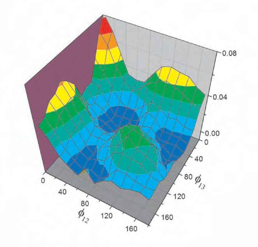
Figure 28: Hadron-hadron-hadron correlation function [60].

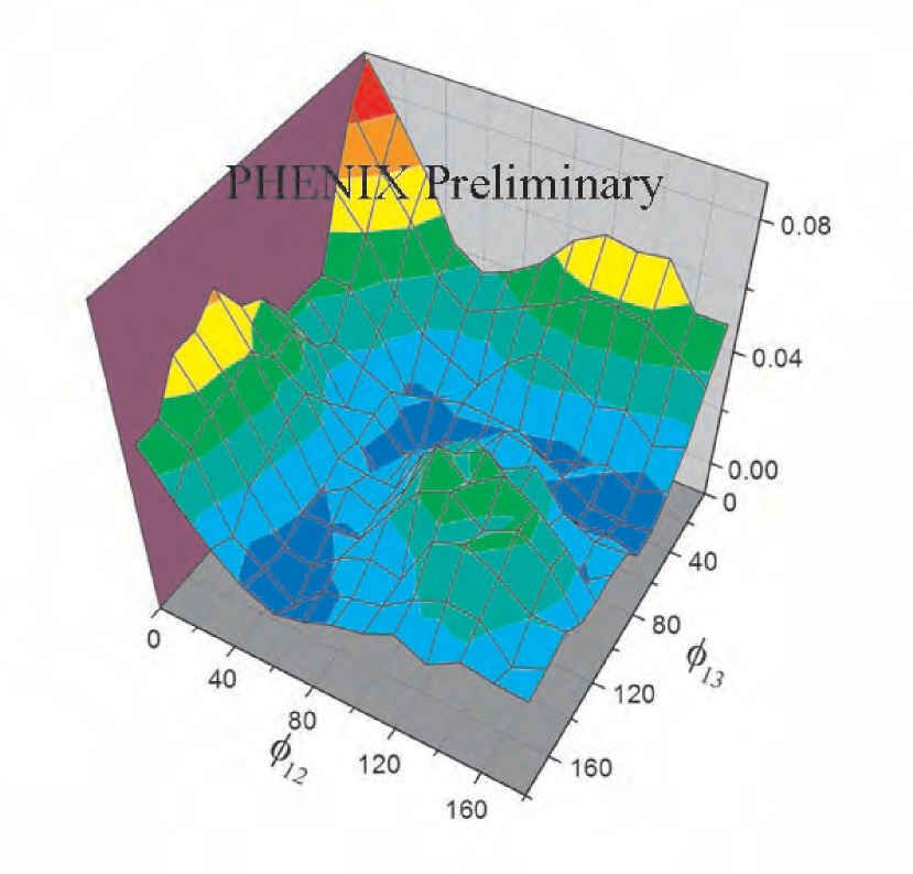
Figure 29: Hadron-meson-meson correlation function [60].

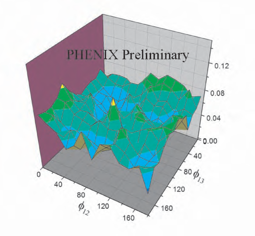
Figure 30: Hadron-baryon-baryon correlation function [60].

Figs. 30 - 30 show three-particle $\Delta\phi$ jet correlation surfaces ($\Delta\phi_{1,2}$ vs. $\Delta\phi_{1,3}$) for a trigger hadron from the range $2.5<p_{T}<$4.0 GeV/c (hadron #1) and two associated hadrons from the range $1.0<p_{T}<$2.5 GeV/c (hadron #2 and #3) [61]. Results are shown for the centrality selection 10-20 %. They show a strong dependence on the flavor (PID) of the associated particle and clearly do not follow the expected patterns for a “normal jet” [61]. Instead, they provide rather compelling evidence for strong modification of the away-side jet. Further detailed quantitative investigations are required to firm up whether or not the tantalizing qualitative features evidenced in Figs. 30 and 30 confirm the presence of conical flow.

5 Epilogue

In summary, the gross elliptic flow patterns observed at RHIC provide compelling evidence for the production and rapid thermalization (less than 1 fm/c after impact) of nuclear matter having an energy density well in excess of an order of magnitude above the critical value required for deconfinement. The universal and fine structure scaling properties of this flow, indicate that this new form of matter behaves like a perfect liquid. The quark number scaling observed at intermediate $p_{T}$s (when the fluid dynamical picture breaks down), indicates that the relevant degrees of freedom are those of constituent or valence quarks. These properties are consistent with those of a strongly coupled plasma with essentially perfect fluid-like properties. Systematic experimental and theoretical efforts are currently underway to quantitatively pin down the thermalization time, EOS and transport properties of this plasma.

References

- [1] Z. Fodor and S. D. Katz, JHEP 0203 (2002) 014
- [2] K. Reidlich, F. Karsch, A. Tawfik, J. Phys. G30: S1271-S1274, 2004
- [3] Gyulassy, Nucl. Phys. A750, 30-63, 2005
- [4] E. Glass Gold et al. Annals of Physics 6, 1 (1959)
- [5] G.F. Chapline, M.H. Johnson, E. Teller, and M.S. Weiss, PRD 8, 4302 (1973)
- [6] W. Scheid, H. Muller, and W. Greiner, PRL 32, 741 (1974)
- [7] H. St cker, J.A. Maruhn, and W. Greiner, PRL 44, 725 (1980)
- [8] For reviews see, e.g., J. Ollitrault, Nucl. Phys. A 638, 195 (1998); A. M. Poskanzer, arXiv:nucl-ex/0110013; S. A. Voloshin, Nucl. Phys. A 715, 379 (2003) .
- [9] H. Stöcker, nucl-th/0406018; J. Casalderrey-Solana et al, hep-ph/0411315; B. Muller et al, Hep-ph/0503158; T. Renk et al, Hep-ph/0509036; these proceedings.
- [10] S. Wang et al., Phys. Rev. C44, 1091 (1991).
- [11] R. Lacey et al., Phys. Rev. Lett. 70, 1224 (1993).
- [12] Roy A. Lacey, Nucl. Phys. A698, 559-563, (2002)
- [13] P. Danielewicz and G. Odyniec, Phys. Lett. B 157, 146 (1985).
- [14] A. M. Poskanzer and S. A. Voloshin, Phys. Rev. C 58, 1671 (1998) [nucl-ex/9805001].
- [15] J.-Y. Ollitrault, Phys. Rev. D 48, 1132 (1993) [hep-ph/9303247].
- [16] J.-Y. Ollitrault, nucl-ex/9711003.
- [17] R. Kotte et al., Eur. Phys. J. A 23, 271 (2005).
- [18] B. Hong et al., Phys. Lett. B 407, 115 (1997); M. Eskef et al., Eur. Phys. J. A 3, 335 (1998)
- [19] Y.V. Kovchegov, K.L. Tuchin, Nucl. Phys. A 708, 413 (2002)
- [20] R.S. Bhalerao, N. Borghini, and J.-Y.Ollitrault, Nucl. Phys. A 727, 373 (2003).
- [21] N. Borghini, P.M. Dinh, and J.-Y. Ollitrault, Phys. Rev. C 64, 054901 (2001).
- [22] C.N. Yang and T.D. Lee, Phys. Rev. 87, 404 (1952); T.D. Lee and C.N. Yang, ibid. 410 (1952)
- [23] W. G. Holzmann et al, nucl-ex/0508010”; N. N. Ajitanand, nucl-ex/0510040; B. Cole, these proceedings (2005).
- [24] B. K. Nandi, G. C. Mishra, B. Mohanty, D. P. Mahapatra and T. K. Nayak, Phys. Lett. B 449, 109 (1999) [nucl-ex/9812004].
- [25] M. Asakawa, H. Minakata and B. Muller, nucl-th/0011031.
- [26] S. A. Voloshin, Phys. Rev. C 62, 044901 (2000) [nucl-th/0004042].
- [27] S. A. Voloshin and W. E. Cleland, Phys. Rev. C 53, 896 (1996) [nucl-th/9509025].
- [28] U. A. Wiedemann, Phys. Rev. C 57, 266 (1998) [nucl-th/9707046].
- [29] H. Heiselberg, Phys. Rev. Lett. 82, 2052 (1999) [nucl-th/9809077].
- [30] M. A. Lisa et al. [E895 Collaboration], Phys. Lett. B 496, 1 (2000) [nucl-ex/0007022].
- [31] S. Voloshin and Y. Zhang, Z. Phys. C 70, 665 (1996) [hep-ph/9407282].
- [32] H. Sorge, Phys. Rev. Lett. 78 2309 (1997) ; ibid. 82 2048 (1999).
- [33] P. Danielewicz et al., Phys. Rev. Lett. 81, 2438 (1998).
- [34] A. Wetzler, private communication (2005)
- [35] P. Danielewicz, Roy Lacey and W. G. Lynch,, Science, 298, 1592-1596, (2002)
- [36] KAOS Collaboration, Z. Phys. A355 (1996)
- [37] C. Pinkenburg et al., Phys. Rev. Lett. 83, 1295 (1999).
- [38] J.-Y. Ollitrault, Phys. Rev. D 46, 229 (1992).
- [39] D. Teaney, J. Lauret, and E.V. Shuryak, nucl-th/ 0011058.
- [40] P. F. Kolb et al., hep-ph/0103234
- [41] T. Hirano et al., these proceedings.
- [42] S. Butsyk (PHENIX), nucl-ex/0510010 (2005).
- [43] R. J. Snellings, Nucl. Phys. A698, 193-198, (2002).
- [44] K. Adcox, (PHENIX Collaboration), Phys. Rev. Lett. 87, 052301 (2001).
- [45] S.S. Adler, (PHENIX Collaboration), Phys. Rev. C 71, 034908 (2005)
- [46] G. Roland, (PHOBOS Collaboration), nucl-ex/0510042, (2005).
- [47] G. Roland, (PHOBOS Collaboration); S. Manly, (PHOBOS Collaboration); H. Masui, (PHENIX Collaboration); M. Oldenburg, (STAR Collaboration); G. Wang, (STAR Collaboration), these proceedings.
- [48] J. Adams et al., (STAR Collaboration), Phys. Rev. C 72, 014904, (2005)
- [49] R. Rapp et al., hep-ph/0510050 (2005).
- [50] S. S. Adler, et al. (PHENIX Collaboration), nucl-ex/0411040, (2004).
- [51] P. F. Kolb, J. Sollfrank, and U. Heinz, Phys. Rev. C 62 054909 (2000).
- [52] S. S. Adler (PHENIX) Phys. Rev. Lett. 94, 232302 (2005)
- [53] R. J. Fries et al., Phys. Rev. Lett. 90, 202303, (2003).
- [54] T. Csörgő, S. V. Akkelin, Y. Hama, B. Lukács and Y. M. Sinyukov, Phys. Rev. C 67, 034904 (2003)
- [55] T. Csörgő and B. Lörstad, Phys. Rev. C 54 (1996) 1390
- [56] M. Csanád, T. Csörgő and B. Lörstad, Nucl. Phys. A 742, 80 (2004)
- [57] M. Csanád, et al., nucl-th/0510027, (2005)
- [58] G.F.Chapline and A.Granik, Nucl. Phys. A459, 681, (1986); A511 747, (1990); D.H.Rischke, H.Stocker and W.Greiner, Phys.Rev. D42, 2283, (1990).
- [59] K. Adcox et al (PHENIX) PRL 88, 022301, 2002; C. Adler et al (STAR) PRL 89, 202301, 2002; S. S. Adler et al (PHENIX) PRL 91 , 072301, 2003; J. Adams et al (STAR) PRL 91, 172302, 2003.
- [60] S.S. Adler et al, nucl-ex/0507004; F. Wang, these proceedings.
- [61] N. N. Ajitanand (PHENIX), nucl-ex/0510040 (2005).