Rapidity distributions around mid-rapidity of strange particles in Pb-Pb collisions at 158 $A$ GeV/$c$

Abstract

The production at central rapidity of $\mathrm{K^{0}_{S}}$, $\mathrm{\Lambda}$, $\Xi$ and $\Omega$ particles in Pb-Pb collisions at 158 $A$ GeV/$c$ has been measured by the NA57 experiment over a centrality range corresponding to the most central 53% of the inelastic Pb-Pb cross section. In this paper we present the rapidity distribution of each particle in the central rapidity unit as a function of the event centrality. The distributions are analyzed based on hydrodynamical models of the collisions.

1 Introduction

Lattice quantum chromodynamic calculations predict a new state of matter of deconfined quark and gluons (quark gluon plasma, QGP) at an energy density exceeding $\sim$ 1 GeV/fm³ [1]. Nuclear matter at high energy density has been extensively studied through ultra-relativistic heavy ion collisions (for recent developements, see reference [2]).

Within the experimental programme with heavy-ion beams at CERN SPS, NA57 is a dedicated experiment for the study of the production of strange and multi-strange particles in Pb-Pb collisions at mid-rapidity [3].

The measurement of strange particle production provides one of the most powerful tools to study the dynamics of the reaction. In particular, an enhanced production of strange particles in nucleus–nucleus collisions with respect to proton–induced reactions was suggested long ago as a possible signature of the phase transition from colour confined hadronic matter to a QGP [4]. The enhancement is expected to increase with the strangeness content of the hyperon. These features were first observed by the WA97 experiment [5] and subsequently confirmed and studied in more detail by the NA57 experiment [6]. Other insights into the reaction dynamics have been inferred from the $p_{\tt T}$ distributions of the strange particles: the study of the transverse expansion of the collision and the $p_{\tt T}$ dependence of the nuclear modification factors have been presented, respectively, in reference [7] and [8].

Rapidity distributions provide a tool to study the longitudinal dynamics; e.g., differences between protons and anti-protons have been interpreted as a consequence of the nuclear stopping [9]. If hyperons, like protons, keep a ‘memory’ of the initial baryon density, then the relative pattern for the rapidity distribution of hyperons and anti-hyperons should resemble that of protons and anti-protons [10].

Hydrodynamical properties of the expanding matter created in heavy ion reactions have been discussed by Landau [11] and Bjorken [12] in theoretical pictures using different initial conditions. In both scenarios, thermal equilibrium is quickly achieved and the subsequent isentropic expansion is governed by hydrodynamics.

2 Data sample

The NA57 experiment has been described in detail elsewhere [7, 13]. The results presented in this paper are based on the analysis of the Pb-Pb data sample collected at 158 $A$ GeV/$c$ (460 M events); the sample analyzed here corresponds to the most central 53% of the inelastic Pb-Pb cross-section. The data have been divided into five centrality classes, labelled as 0,1,2,3 and 4 from the most peripheral to the most central, according to the value of the charged particle multiplicity sampled at central rapidity by a dedicated silicon microstrip detector.

The procedure to measure the multiplicity distribution and to determine the centrality of the collision for each class is described in reference [14]. The fractions of the inelastic cross-section for each of the five classes, determined assuming an inelastic Pb-Pb cross-section of 7.26 barn (as calculated with the Glauber model), are given in table 1.

Table 1: Centrality ranges for the five classes.

Class	$4$	$3$	$2$	$1$	$0$
$\sigma/\sigma_{inel}$   (%)	0 to 4.5	4.5 to 11	11 to 23	23 to 40	40 to 53

3 Analysis and results

A detailed description of the particle selection procedure, as well as of the corrections for geometrical acceptance and for detector and reconstruction inefficiencies, can be found in reference [7]. Here we describe the principal features of the analysis.

The selection of strange particles was accomplished by reconstructing their weak decays into final states containing only charged particles:

$$\begin{array}[]{lllllll}\mathrm{K^{0}_{S}}&\rightarrow&\pi^{+}+\pi^{-}&&\Lambda&\rightarrow&p+\pi^{-}\\ \\ \Xi^{-}&\rightarrow&\Lambda+\pi^{-}&&\Omega^{-}&\rightarrow&\Lambda+K^{-}\\ &&\makebox[0.0pt][l]{\rule{3.30002pt}{0.0pt}\rule[2.36806pt]{0.44006pt}{6.6736pt}}\rightarrow p+\pi^{-}&&&&\makebox[0.0pt][l]{\rule{3.30002pt}{0.0pt}\rule[2.36806pt]{0.44006pt}{6.6736pt}}\rightarrow p+\pi^{-}\\ \end{array}$$ (1)

and their corresponding charge conjugates for antihyperons. Geometric and kinematic constraints were used to obtain high purity strange particle samples: the total amount of combinatorial background is estimated to be 0.7%, 0.3% and 1.2% for $\mathrm{K^{0}_{S}}$, $\mathrm{\Lambda}$ and $\mathrm{\overline{\Lambda}}$ respectively, and less than 5% for $\Xi$ and $\Omega$.

An event by event procedure, using a GEANT-based [15] Monte Carlo simulation of the apparatus, was applied to correct the data for geometrical acceptance and for detector and reconstruction inefficencies. This procedure, which is very accurate but rather time consuming, assigns a weight to each reconstructed particle and was specifically developed for rare signals such as $\Omega$ and $\Xi$. The same procedure was also applied to small fractions of the much more abundant $\mathrm{K^{0}_{S}}$ and $\Lambda$ samples. The selected particles have been sampled uniformly over the whole data taking period; the sizes of those subsamples were chosen in order to reach a statistical accuracy better than the limits imposed by the systematic errors.

Acceptance regions have been refined off-line in such a way to excluded from the final sample the border regions where the correction factors would have larger systematic errors. The selected regions of the transverse momentum vs. rapidity plane are shown in figure 1.

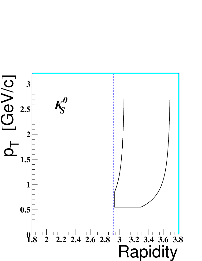
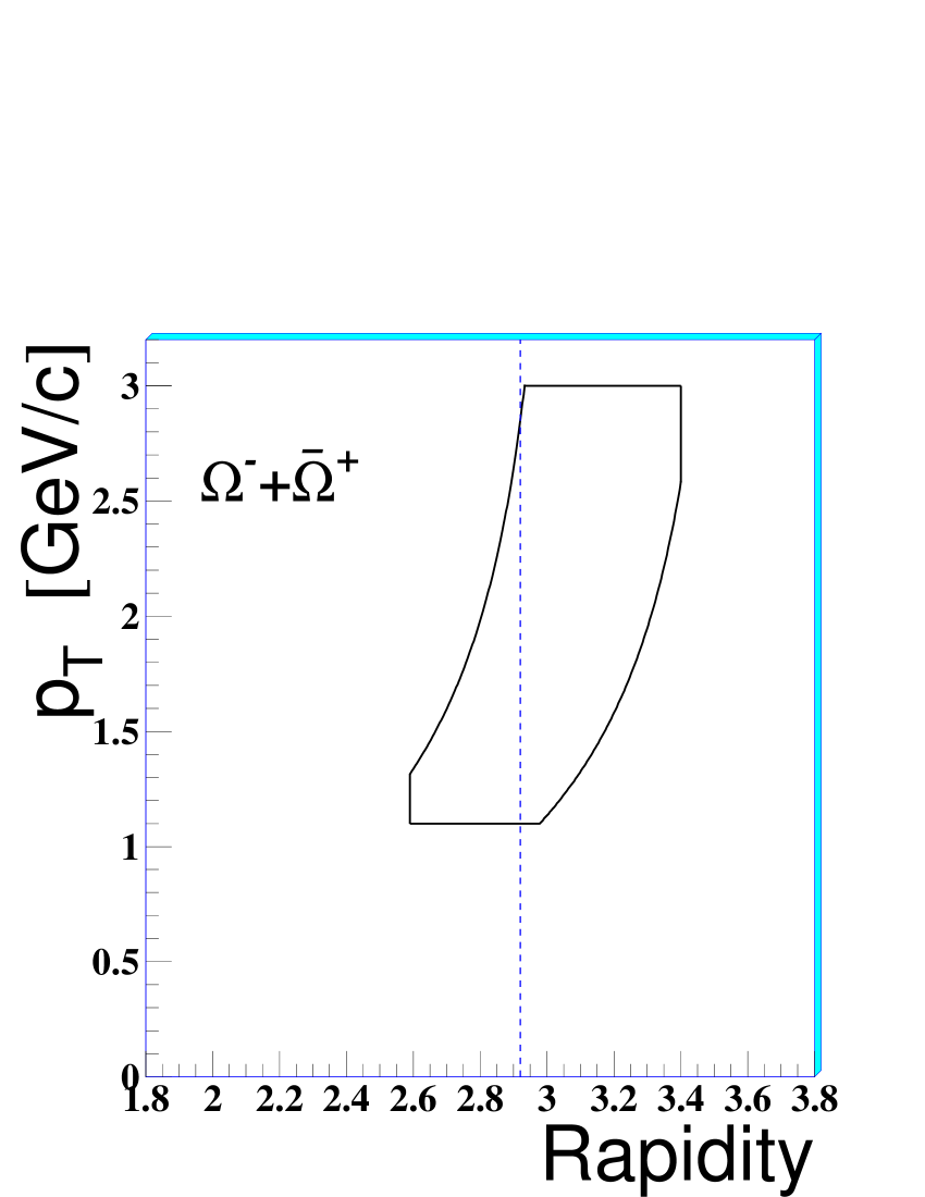
Figure 1: The $y$–$p_{\tt T}$ acceptance windows. Dashed lines show the position of mid-rapidity ($y_{cm}=2.92$).

Extensive checks were performed by comparing real and Monte Carlo distributions for several geometrical and kinematical parameters, in particular those used in the particle selection procedure. In all cases a good agreement between MC and data has been found [7, 16].

The double-differential distribution for each particle species has been parameterized using the expression

$$\frac{d^{2}N}{p_{\tt T}dp_{\tt T}dy}\propto\frac{dN}{dy}\hskip 2.84526pt\cdot\exp\left(-\frac{\sqrt{m^{2}+p_{\tt T}^{2}}}{T_{app}}\right)$$ (2)

where the inverse slope parameter $T_{app}$ (‘apparent temperature’) has been extracted by means of a maximum likelihood fit of equation 2 to the data [7]. By using equation 2 we can extrapolate the rapidity distribution measured in the selected acceptance window down to $p_{\tt T}=0$:

$$\frac{dN}{dy}=\int_{0}^{\infty}{\rm d}p_{\tt T}\frac{{\rm d}^{2}N}{{\rm d}p_{\tt T}{\rm d}y}.$$ (3)

The contribution of the extrapolation procedure to the systematic errors on $\frac{dN}{dy}$ has been evaluated using an alternative parameterization for the $p_{\tt T}$ dependence of the invariant double-differential distribution: instead of the single exponential in equation 2, the blast-wave model, a hydrodynamics-inspired model with a kinetic freeze-out temperature $T_{f}$ and a linear transverse flow velocity field $\beta_{\perp}(r)$ [17], was used with freeze-out parameters $T_{f}=144$ MeV and $<\beta_{\perp}>=0.38$ which we determined from the blast-wave analysis of the $p_{\tt T}$ spectra [7]. This alternative procedure does not affect the shape of the $\frac{dN}{dy}$ distributions but only the absolute values of the extracted yields; the yield of the $\mathrm{K^{0}_{S}}$ meson increases by $6\%$, that of the $\mathrm{\Lambda}$ hyperon remains unchanged, those of the $\Xi$ and $\Omega$ hyperons decrease by $5\%$ and $20\%$, respectively. This results in the main source of systematic uncertainty for the $\Omega$ hyperon.

3.1 Results in the centrality range 0-53%

The measured rapidity distributions for the centrality range corresponding to the most central 53% of the Pb-Pb inelastic cross-section (total sample) are shown in figure 2 with closed symbols. For all hyperons the rapidity distributions are found to be symmetric with respect to the rapidity of the centre of mass (‘mid-rapidity’) within the statistical errors. A similar conclusion cannot be drawn for $\mathrm{K^{0}_{S}}$ since our acceptance coverage does not extend to backward rapidity.

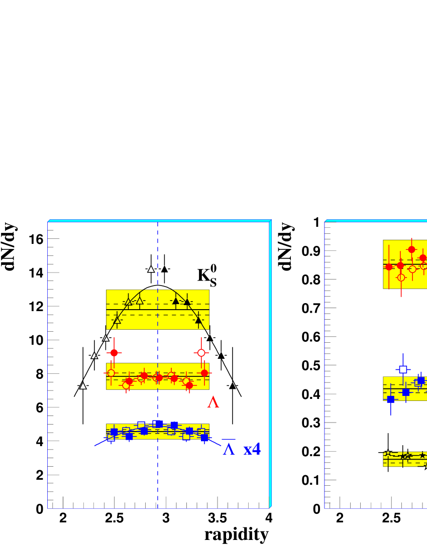
Figure 2: Rapidity distributions of strange particles in the most central 53% of Pb-Pb interactions at 158 $A$ GeV/$c$. Closed symbols are measured data, open symbols are measured points reflected around mid-rapidity. The $\mathrm{\overline{\Lambda}}$ and $\mathrm{\overline{\Xi}^{+}}$ results have been scaled by factors 4 and 2, respectively, for dispaly purposes. The superimposed boxes show the yields measured in one unit of rapidity (as published in references [6, 18]) with the dashed and full lines indicating the statistical and systematic errors, respectively.

The symmetry of the Pb-Pb colliding system allows us to reflect the rapidity distributions around mid-rapidity. In figure 2 open symbols are used to plot the measured points after such a reflection.

The rapidity distributions of $\mathrm{\Lambda}$, $\mathrm{\Xi^{-}}$, $\mathrm{\overline{\Xi}^{+}}$and $\Omega$ are compatible, within the error bars, with being flat within the NA57 acceptance window. For the $\mathrm{K^{0}_{S}}$ and $\mathrm{\overline{\Lambda}}$ spectra, on the other hand, we observe a rapidity dependence. The rapidity distributions for these particles are well described by Gaussians centred at mid-rapidity.

Table 2: Absolute yields in one unit of rapidity calculated by means of maximum likelihood fits. The first error is statistical, the second is systematic. Values of the $\chi^{2}/ndf$ for the measured $dN/dy$ distributions calculated assuming $dN/dy$ constant and equal to the absolute yields are also quoted.

	$\int^{y_{cm}+0.5}_{y_{cm}-0.5}{\frac{dN}{dy}\,dy}$	$\chi^{2}/ndf$
$\mathrm{K^{0}_{S}}$	$11.8\pm 0.3\pm 1.2$	$29/6$
$\mathrm{\overline{\Lambda}}$	$1.14\pm 0.03\pm 0.12$	$12/6$
$\mathrm{\Lambda}$	$7.84\pm 0.21\pm 0.78$	$3.9/6$
$\mathrm{\Xi^{-}}$	$0.852\pm 0.015\pm 0.085$	$3.7/7$
$\mathrm{\overline{\Xi}^{+}}$	$0.209\pm 0.007\pm 0.021$	$3.6/5$
$\mathrm{\Omega^{-}}$+ $\mathrm{\overline{\Omega}^{+}}$	$0.172\pm 0.013\pm 0.026$	$5.0/4$

The total yields integrated over one unit of rapidity as reported in references [6, 18] are also shown in figure 2 as shaded bands superimposed to the corresponding rapidity distributions. In these bands the dotted and full lines represent, respectively, the statistical and the systematic errors. These yields are calculated with a maximum likelihood fit using the Gaussian parameterization of $dN/dy$ for $\mathrm{K^{0}_{S}}$ and $\mathrm{\overline{\Lambda}}$, and a flat $dN/dy$ for all other particles. The numerical values of the yields are reported in table 2 along with their errors .

The Gaussian parameters which minimize the $\chi^{2}$ of the $\mathrm{K^{0}_{S}}$ and $\mathrm{\overline{\Lambda}}$ distributions are given in table 3.

Table 3: Results of fits with a Gaussian to the rapidity distributions of $\mathrm{K^{0}_{S}}$ and $\mathrm{\overline{\Lambda}}$.

	$\frac{dN}{dy}\left|{}_{y=y_{cm}}\right.$	$\sigma$	$\chi^{2}/ndf$
$\mathrm{K^{0}_{S}}$	$13.2\pm 0.4$	$0.69\pm 0.07$	$2.5/5$
$\mathrm{\overline{\Lambda}}$	$1.22\pm 0.04$	$0.83\pm 0.22$	$3.0/5$

3.2 Comparison with NA49 results

The large acceptance NA49 experiment has measured the rapidity distributions of a number of particle species over a broad rapidity range ($\approx 3$ units of rapidity centred around mid-rapidity) in central Pb-Pb collisions [19]. The $\mathrm{\Lambda}$ rapidity distribution measured by NA49 is flat over the experiment’s $y$-coverage and the $\mathrm{\overline{\Lambda}}$ distribution has been fitted to a Gaussian with a width of $0.95\pm 0.05$ [20], compatible with our findings. NA49 has fitted the rapidity distributions of negatively and positively charged kaons with a two-Gaussian parameterization [21]. Assuming the $\mathrm{K^{0}_{S}}$ to be an average of $\mathrm{K^{-}}$ and $\mathrm{K^{+}}$, and taking the ($\mathrm{K^{-}}$+$\mathrm{K^{+}}$)/2 average of the NA49 fitted parameters one obtains in our rapidity range ($2.93<y<3.70$) $rms=0.219$  to be compared with $rms=0.221$ of our measured distribution. For the multi-strange $\Xi$ and $\Omega$ hyperons, our rapidity distributions are compatible within the error bars both with being flat and with the shapes of the NA49 fits [22, 23].

In conclusion, there is a fairly good agreement between the two experiments as far as the shape of the rapidity distributions are concerned. On the other hand a systematic discrepancy on the values of the yields is found relative to the NA49 results, which are lower for all particles by about 25-30% [24]. The origin of such a discrepancy has not yet been understood despite the joint efforts of the two collaborations.

3.3 Centrality dependence

In figures 5 and 5 we show the centrality dependence of the rapidity distributions for $\mathrm{K^{0}_{S}}$ and $\mathrm{\overline{\Lambda}}$, respectively. As in figure 2, the shaded bands represent our determination of the yield in one unit of rapidity, according to the maximum likelihood fit [6, 18], with the dotted and full lines indicating the statistical and systematic errors, respectively. Gaussian $\chi^{2}$ fits to the spectra are also superimposed, with the fit parameters reported in table 4. For both particles, the width of the rapidity distributions is constant within the errors in the five centrality classes (i.e. from 40–53% to 0–4.5%, see table 1).

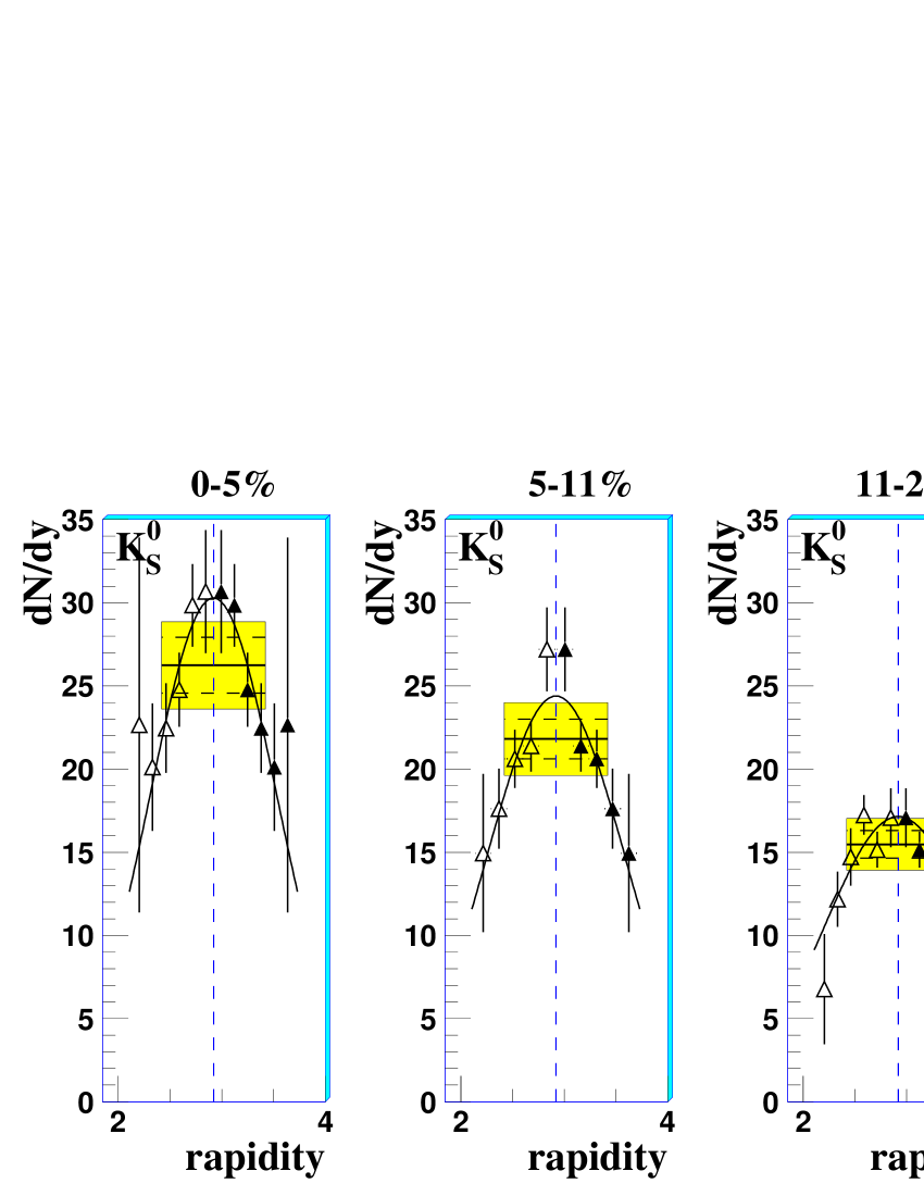
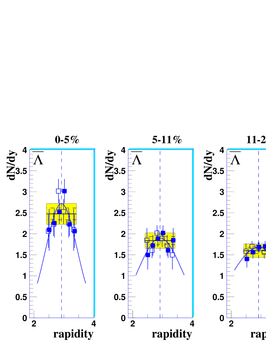
Figure 3: Rapidity distributions of $\mathrm{K^{0}_{S}}$ for the five centrality classes.

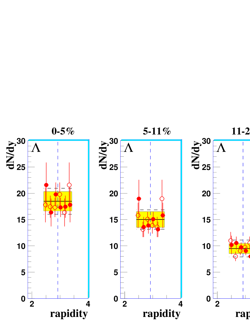
Figure 4: Rapidity distributions of $\mathrm{\overline{\Lambda}}$ for the five centrality classes.

Figure 5: Rapidity distributions of $\mathrm{\Lambda}$ for the five centrality classes.

The rapidity distributions in the five centrality classes of $\mathrm{\Lambda}$, $\mathrm{\Xi^{-}}$ and $\mathrm{\overline{\Xi}^{+}}$ are shown in figures 5, 8 and 8, respectively. For statistical reasons the rapidity distributions of $\mathrm{\Omega^{-}}$+$\mathrm{\overline{\Omega}^{+}}$ have been calculated in three centrality classes instead of five: $0+1$, $2$ and $3+4$ and they are shown in figure 8. In all the centrality classes, the rapidity distribution of the $\mathrm{\Lambda}$ hyperon is consistent with being flat over the considered range. In the same rapidity range, the $\mathrm{\overline{\Lambda}}$ distribution varies by about 40% (class 4). It is likely that the $\mathrm{\Lambda}$ hyperon rapidity distribution reflects the overall net baryon number distribution. The same behaviour was observed for the $y$ distribution of protons in central Pb-Pb collisions at the same energy by the NA49 experiment [10]. The $\mathrm{\Xi^{-}}$ distributions are found to be flat in one unit of rapidity like the $\mathrm{\Lambda}$ distributions. For the rare $\mathrm{\overline{\Xi}^{+}}$and $\Omega$ particles, the NA57 collected statistics do not allow us to observe significant deviations from a flat distribution in our limited rapidity range.

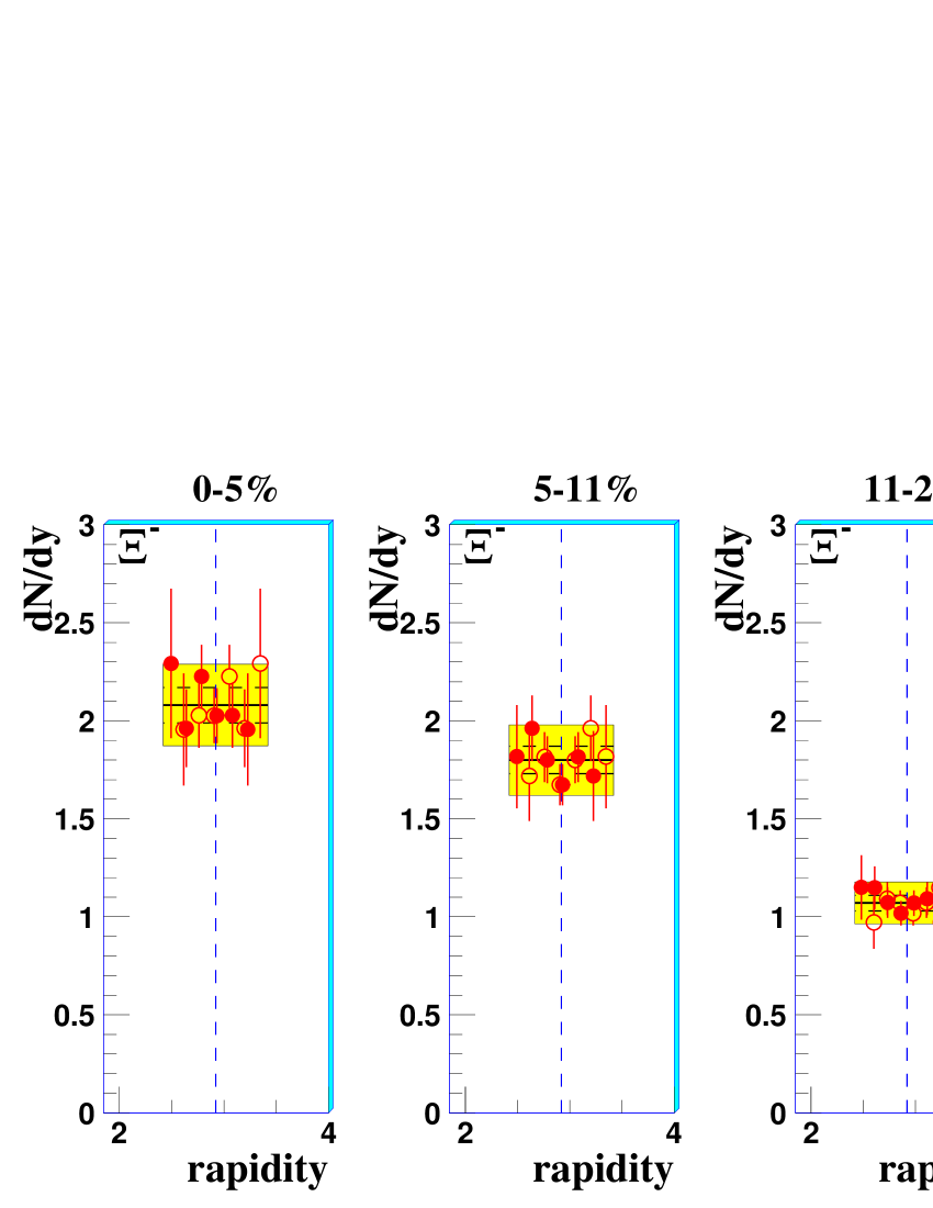
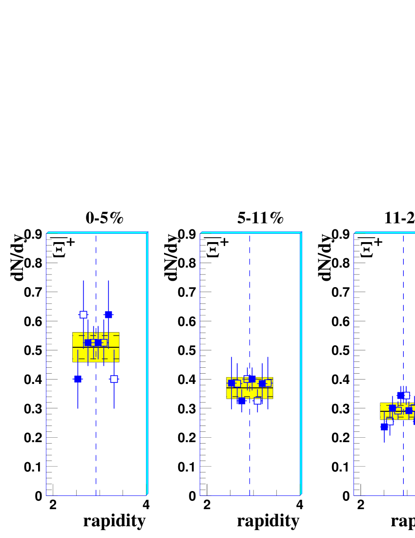
Figure 6: Rapidity distributions of $\mathrm{\Xi^{-}}$ for the five centrality classes.

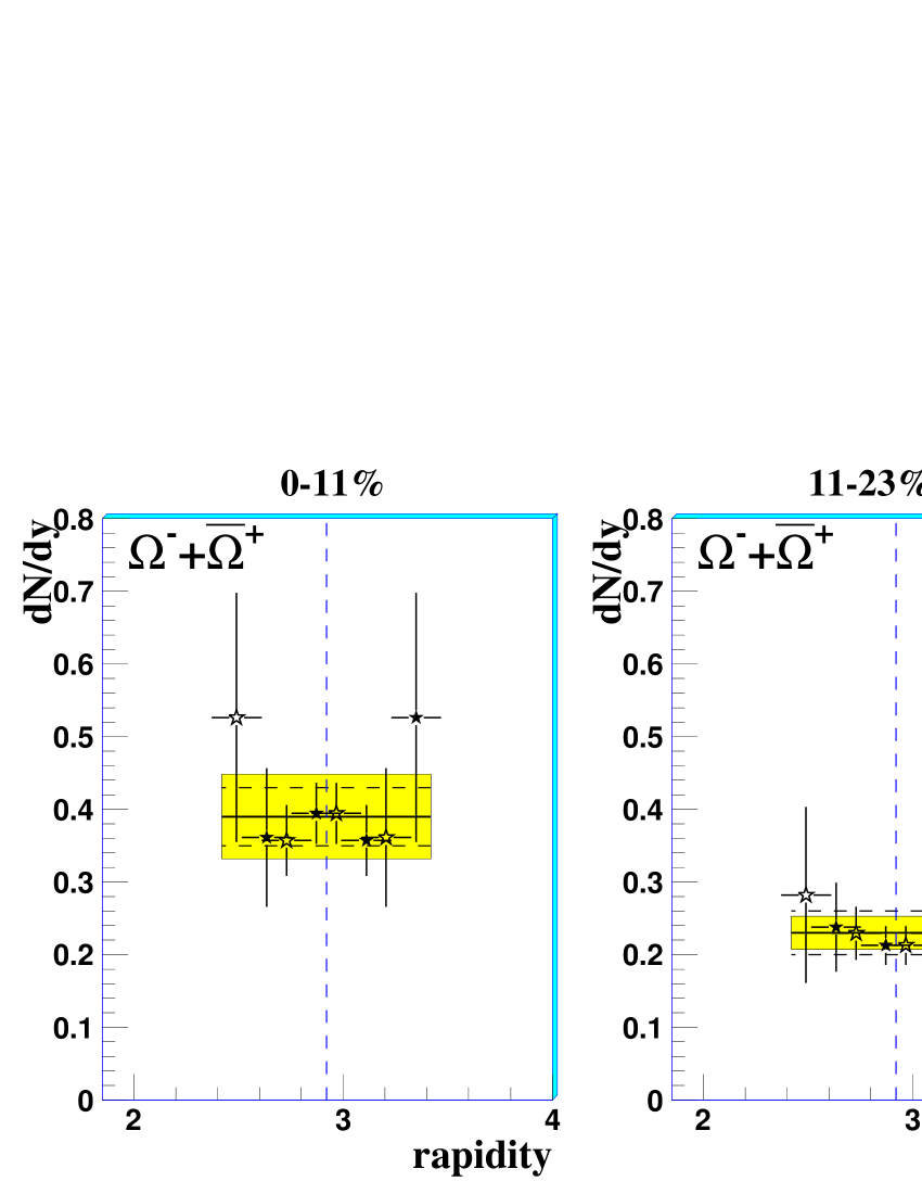
Figure 7: Rapidity distributions of $\mathrm{\overline{\Xi}^{+}}$ for the five centrality classes.

Figure 8: Rapidity distributions of $\mathrm{\Omega^{-}}$+$\mathrm{\overline{\Omega}^{+}}$ for central (0-11%), semi-central (11-23%) and semi-peripheral (23-53%) collisions.

Table 4: Results of fits with a Gaussian to the rapidity distributions of $\mathrm{K^{0}_{S}}$ and $\mathrm{\overline{\Lambda}}$ for the five centrality classes defined in table 1.

		4	3	2	1	0
$\mathrm{K^{0}_{S}}$	$\frac{dN}{dy}\left|{}_{y=y_{cm}}\right.$	$30.3\pm 2.2$	$24.4\pm 1.6$	$17.2\pm 0.9$	$9.4\pm 0.6$	$3.3\pm 0.4$
	$\sigma$	$0.61\pm 0.12$	$0.67\pm 0.13$	$0.72\pm 0.13$	$0.61\pm 0.11$	$0.71\pm 0.34$
	$\chi^{2}/ndf$	$1.2/4$	$2.4/3$	$5.2/4$	$1.9/5$	$2.4/4$
$\mathrm{\overline{\Lambda}}$	$\frac{dN}{dy}\left|{}_{y=y_{cm}}\right.$	$2.72\pm 0.20$	$1.90\pm 0.13$	$1.68\pm 0.09$	$0.90\pm 0.06$	$0.44\pm 0.05$
	$\sigma$	$0.52\pm 0.14$	$0.73\pm 0.34$	$0.9\pm 0.5$	$0.61\pm 0.20$	$0.48\pm 0.19$
	$\chi^{2}/ndf$	$2.6/4$	$2.4/4$	$1.14/3$	$1.18/4$	$7.0/5$

The values of the yield in one unit of rapidity around mid-rapidity as a function of the centrality of the collision are given in table 5 for all the particles.

Table 5: Strange particle yields in one unit of rapidity around mid-rapidity, $\int^{y_{cm}+0.5}_{y_{cm}-0.5}{\frac{dN}{dy}\,dy}$, for the five centrality classes defined in table 1. Statistical (first) and systematic (second) errors are also quoted.

	4	3	2	1	0
$\mathrm{K^{0}_{S}}$	$26.0\pm 1.7\pm 2.6$	$21.6\pm 1.2\pm 2.2$	$15.3\pm 0.8\pm 1.6$	$8.1\pm 0.5\pm 0.8$	$3.05\pm 0.33\pm 0.31$
$\mathrm{\overline{\Lambda}}$	$2.44\pm 0.14\pm 2.4$	$1.81\pm 0.10\pm 0.18$	$1.58\pm 0.07\pm 0.16$	$0.80\pm 0.04\pm 0.08$	$0.41\pm 0.03\pm 0.04$
$\mathrm{\Lambda}$	$18.5\pm 1.1\pm 1.8$	$15.0\pm 0.8\pm 1.5$	$9.5\pm 0.5\pm 0.9$	$5.19\pm 0.29\pm 0.51$	$2.30\pm 0.22\pm 0.23$
$\mathrm{\Xi^{-}}$	$2.08\pm 0.09\pm 0.21$	$1.80\pm 0.07\pm 0.18$	$1.07\pm 0.04\pm 0.11$	$0.52\pm 0.02\pm 0.05$	$0.181\pm 0.013\pm 0.018$
$\mathrm{\overline{\Xi}^{+}}$	$0.51\pm 0.04\pm 0.05$	$0.37\pm 0.03\pm 0.04$	$0.29\pm 0.02\pm 0.03$	$0.14\pm 0.01\pm 0.01$	$0.045\pm 0.007\pm 0.004$
$\Omega$	$0.39\pm 0.04\pm 0.06$		$0.23\pm 0.03\pm 0.03$	$0.069\pm 0.012\pm 0.010$

4 Longitudinal dynamics

The transverse dynamics of the collisions have been studied in reference [7] from the analysis of the transverse momentum distributions of the strange particles in the frame-work of the blast-wave model [17]. The rapidity distributions can be used to extract information about the longitudinal dynamics. We use an approach outlined in reference [17] (i.e., the same blast-wave model used for the study of the transverse dynamics) and [25], where, respectively, Bjorken and Landau hydrodynamics [12, 11] are folded with a thermal distribution of the fluid elements.

In figure 9 the observed rapidity distributions are compared with the expectation for a stationary thermal source and with a longitudinally boost-invariant superposition of multiple isotropic, locally-thermalized sources (i.e. Bjorken hydrodynamics). Each locally thermalized source is modelled by an $m_{\tt T}$-integrated Maxwell-Boltzmann distribution with the rapidity dependence of the energy, $E=m_{\tt T}\cosh(\eta)$ explicitly included

$$\frac{dN_{th}}{d\eta}(\eta)=AT_{f}^{3}(\frac{m^{2}}{T_{f}^{2}}+\frac{m}{T_{f}}\frac{2}{\cosh\eta}+\frac{2}{\cosh^{2}\eta})\exp(-\frac{m}{T_{f}}\cosh\eta)\;,$$ (4)

where $T_{f}$ is the freeze-out temperature and $m_{\tt T}=\sqrt{p_{\tt T}^{2}+m^{2}}$.

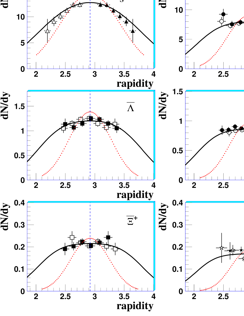
Figure 9: Rapidity distributions of strange particles for the centrality range corresponding to the most central 53% of the inelastic Pb-Pb cross-section as compared to the thermal model calculation of equation 4 (dotted lines, in red) and a thermal model with longitudinal flow (full lines, in black).

The distributions are integrated over source element rapidity to extract the maximum longitudinal flow, $\eta_{max}$

$$\frac{dN}{dy}=\int^{\eta_{max}}_{-\eta_{max}}{\frac{dN_{th}}{d\eta}(y-\eta)\,d\eta}\newline \beta_{L}=\tanh{\eta_{max}}$$ (5)

where $\beta_{L}$ is the maximum longitudinal velocity in units of $c$. The average longitudinal flow velocity is evaluated as $<\beta_{L}>=\tanh(\eta_{max}/2)$. A simultaneous fit of the function defined by equation 5 to the rapidity distributions of the strange particles gives $<\beta_{L}>=0.42\pm 0.03$ with $\chi^{2}/ndf=28.2/32$. The freeze-out temperature has been fixed to the value $T_{f}=144$ MeV obtained, for the most central 53% of the inelastic Pb-Pb collisions, from the analysis of the transverse mass spectra of the same group of particles [7]. In the same analysis the average transverse flow velocity has been determined to be $<\beta_{\perp}>=0.38\pm 0.02$, i.e. slightly less than the longitudinal velocity determined in this analysis; this indicates substantial stopping of the incoming nuclei as a consequence of the collision.

In principle, also the freeze-out temperature can be fitted from the rapidity distributions along with the longitudinal velocity. However, the sensitivity to the freeze-out temperature is very limited. For instance, changing $T_{f}$ from 144 to 120 MeV results in only a 2% increase of $<\beta_{L}>$. The partial contributions to the total $\chi^{2}$ from the individual particle rapidity spectra are given in table 6. Within our uncertanties, we do not observe any particle to deviate from the common description given by a collective longitudinal flow superimposed to the thermal motion. A combined fit performed only to the $\mathrm{K^{0}_{S}}$ and $\mathrm{\overline{\Lambda}}$ rapidity distributions yields a smaller value of the flow, i.e. $<\beta_{L}>\simeq 0.36\pm 0.03$. It is worth noting that the flattening of the rapidity spectra with increasing particle mass, which is also observed in the data, is due in the model to the collective dynamics: all particles are driven by the flow with the same velocity independently of their masses.

Table 6: Partial contributions to the $\chi^{2}$ of the best-fit to the thermal model with longitudinal flow, equation 5. The $\chi^{2}/ndf$ of the global fit is 28.2/33, since there are six normalization constants (the factors $A$ in equation 5) and the parameter $\beta_{L}$.

particle	n. of points	$\chi^{2}$
$\mathrm{K^{0}_{S}}$	7	5.1
$\mathrm{\overline{\Lambda}}$	7	3.6
$\mathrm{\Lambda}$	7	6.7
$\mathrm{\Xi^{-}}$	8	4.5
$\mathrm{\overline{\Xi}^{+}}$	6	3.1
$\Omega$	5	5.2
tot	40	28.2

In Landau hydrodynamics, the amount of entropy ($dS$) contained within a (fluid) rapidity $d\eta$ is given by [11]

$$\frac{dS}{d\eta}=\pi R^{2}ls_{0}\;\beta c_{s}\exp[\beta\omega_{f}]\left[I_{0}(q)-\frac{\beta\omega_{f}}{q}I_{1}(q)\right]$$ (6)

where $q=\sqrt{\omega_{f}^{2}-c_{s}^{2}\eta^{2}}$, $\omega_{f}=\ln(T_{f}/T0)$, $c_{s}$ is the velocity of sound in the medium, $T_{0}$ is the initial temperature, $\eta$ is the rapidity, $R$ is the radius of the nuclei, $2l$ is the initial length, $s_{0}$ is the initial entropy density, $2\beta=(1-c_{s}^{2})/c_{s}^{2}$ and $I_{0}$, $I_{1}$ are Bessel functions. The quantity $\pi R^{2}ls_{0}$ is used to normalize the spectra at mid-rapidity. The particle rapidity distribution is obtained, as for the Bjorken case, as a superpositon of the multiplicity density in rapidity space ($dN/d\eta\propto dS/d\eta$) with a thermal distribution of the fluid elements,

$$\frac{dN}{dy}\propto\int\frac{dN}{d\eta}\frac{dN_{th}}{d\eta}(y-\eta)\,d\eta$$ (7)

In the Landau model the width of the rapidity distribution is sensitive to the velocity of sound and to the ratio of the freeze-out temparature to the initial temperature. While integrating over $\eta$ in equation 5, the range of $\eta$ is treated as a parameter in case of Bjorken hydrodynamics; moreover in the Bjorken case (equation 5) the factor $dN/d\eta$, which appears in equation 7, has been included in the overall normalization factor $A$ since the entropy density $dS/d\eta$ is independent of the rapidity, in accordance with the assumption of boost invariance along the longitudinal direction [12]. In the case of Landau hydrodynamics, the integration limit is fixed by $\eta_{max}=-\eta_{min}=\ln(T_{0}/Tf)/c_{s}$  and the multiplicity density in $\eta$ space ($dN/d\eta$) is written explicitly in the $\eta$ integration (equation  7). Landau hydrodynamics can also reproduce simultaneously the distributions for all the strange particles considered ($\chi^{2}/ndf\simeq$ 28/32) but we are not able to put stringent constraints on both the velocity of sound and the ratio $T_{f}/T_{0}$. The confidence level contours in the $c_{s}^{2}$ vs. $\frac{T_{f}}{T_{0}}$ parameter space are shown in figure 10. For instance, the hypothesys of a perfect gas (i.e. $c_{s}^{2}=1/3$) would result (at the 3$\sigma$ confidence level) in either $T_{f}/T_{0}\approx 0$ or $T_{f}/T_{0}\approx 0.6$. In fact, two physical regions are constrained at the 3$\sigma$ confidence level, the first located at small values of $T_{f}/T_{0}$ and the second between 0.5 and 0.8; on the other hand, the region at $c_{s}^{2}>1/3$ is unphysical. Both physical regions span over the full range $0<c_{s}^{2}<1/3$.

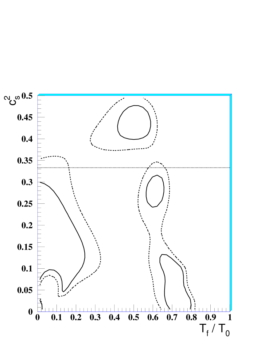
Figure 10: The square of the velocity of sound in the medium (in unit of $c^{2}$) versus the ratio of the freeze-out temperature to the inital temperature. The 1$\sigma$ (full curves) and the 3$\sigma$ (dashed curves) confidence contours are shown. The dotted line at $c_{s}^{2}=1/3$ show the ideal gas limit.

5 Conclusions

We have measured the $dN/dy$ distributions of high purity samples of $\mathrm{K^{0}_{S}}$, $\mathrm{\Lambda}$, $\Xi$ and $\Omega$ particles produced at central rapidity in Pb-Pb collisions at 158 $A$ GeV/$c$ over a wide centrality range of collision (i.e. the most central 53% of the Pb-Pb inelastic cross-section).

In the unit of rapidity around mid-rapidity covered by NA57, we have performed fits to the $dN/dy$ distributions of $\mathrm{K^{0}_{S}}$ and $\mathrm{\overline{\Lambda}}$ using a Gaussian parameterization: the resulting widths are compatible with each other and constant as a function of centrality.

Contrary to $\mathrm{\overline{\Lambda}}$, the $\mathrm{\Lambda}$ spectra are flat to good accurancy in the range of rapidity and centrality considered; this would indicate that the $\mathrm{\Lambda}$ hyperon conserves “memory” of the initial baryon density.

The rapidity distributions of the $\Omega$ particle are found to be flat within the errors in one unit of rapidity for central (0-11%) and peripheral (23-53%) collisions.

Boost-invariant Bjorken hydrodynamics can describe simultaneously the rapidity spectra of all the strange particles under study with $\chi^{2}/ndf\approx 1$, yielding an average longitudinal flow velocity $<\beta_{L}>=0.42\pm 0.03$, sligthly larger than the measured transverse flow. The isotropic collective expansion of the system suggests large nuclear stopping.

A fairly good description is also provided by Landau hydrodynamics, which allows us to put constraints in the parameter space of the velocity of sound in the medium and the ratio of the freeze-out temperature to the initial temperature.

References

References

- [1] Karsch F 2002 Lect. Notes Phys. 583 209
- [2] Quark Matter Conference Proceedings 2004 J. Phys. G: Nucl. Phys.30 S633-S1430
- [3] Caliandro R et al., NA57 proposal, 1996 CERN/SPSLC 96-40, SPSLC/P300
- [4] Rafelski J and Müller B 1982 Phys. Rev. Lett.48 1066 Rafelski J and Müller B 1986 Phys. Rev. Lett.56 2334
- [5] Andersen E et al. 1999 Phys. Lett.B 449 401 Antinori F et al. 1999 Nucl. Phys.A 661 130c
- [6] Bruno G E et al. 2004 J. Phys. G: Nucl. Phys.30 S717-S724
- [7] Antinori F et al. 2004 J. Phys. G: Nucl. Phys.30 823-840
- [8] Antinori F et al. 2005 Phys. Lett.B 623 17-25
- [9] Busza W and Goldhaber A 1984 Phys. Lett.B 139 235
- [10] Appelshäuser H et al. 1999 Phys. Rev. Lett.82 2471
- [11] Landau L D 1953 Izv. Akad. Nauk. SSSR 17 51 Belenkij S and Landau L D 1955 Usp. Fiz. Nauk. 56 309 Belenkij S and Landau L D 1956 Nuovo Cimento(suppl.) 3 15
- [12] Bjorken J D 1983 Phys. Rev.D 27 140
- [13] Manzari V et al. 1999 J. Phys. G: Nucl. Phys.25 473 Manzari V et al. 1999 Nucl. Phys.A 661 761c
- [14] Carrer N et al. 2001 J. Phys. G: Nucl. Phys.27 391 Antinori F et al. 2005 J. Phys. G: Nucl. Phys.31 321-335
- [15] GEANT, CERN Program Library Long Writeup W5013
- [16] Fanebust K et al. 2002 J. Phys. G: Nucl. Phys.28 160
- [17] Schnedermann E, Sollfrank J and Heinz U 1993 Phys. Rev.C 48 2462-2475
- [18] Antinori F et al. 2004 Phys. Lett.B 595 68-74
- [19] Blume C et al. 2005 J. Phys. G: Nucl. Phys.31 S685-S691
- [20] Anticic T et al. 2004 Phys. Rev. Lett.93 022302
- [21] Afanasiev S V et al. 2002 Phys. Rev.C 66 054902
- [22] Afanasiev S V et al. 2002 Phys. Lett.B 538 275-281
- [23] Alt C et al. Alt C et al. 2005 Phys. Rev. Lett.94 192301
- [24] Elia D et al. 2004 J. Phys. G: Nucl. Phys.30 S1329-S1332
- [25] Mohanty B and Alam J 2003 Phys. Rev.C 68 064903
- [26] Srivastava D K, Alam J, Chakrabarty S, Raha S and Sinha B 1993 Ann. Phys. 228 104