Systematic study of three-nucleon force effects
in the cross section of the deuteron-proton breakup at 130 MeV

Abstract

High precision cross-section data of the deuteron-proton breakup reaction at 130 MeV are presented for 72 kinematically complete configurations. The data cover a large region of the available phase space, divided into a systematic grid of kinematical variables. They are compared with theoretical predictions, in which the full dynamics of the three-nucleon (3$N$) system is obtained in three different ways: realistic nucleon-nucleon ($NN$) potentials are combined with model 3$N$ forces (3NF’s) or with an effective 3NF resulting from explicit treatment of the $\Delta$-isobar excitation. Alternatively, the chiral perturbation theory approach is used at the next-to-next-to-leading order with all relevant $NN$ and 3$N$ contributions taken into account. The generated dynamics is then applied to calculate cross-section values by rigorous solution of the 3$N$ Faddeev equations. The comparison of the calculated cross sections with the experimental data shows a clear preference for the predictions in which the 3NF’s are included. The majority of the experimental data points is well reproduced by the theoretical predictions. The remaining discrepancies are investigated by inspecting cross sections integrated over certain kinematical variables. The procedure of global comparisons leads to establishing regularities in disagreements between the experimental data and the theoretically predicted values of the cross sections. They indicate deficiencies still present in the assumed models of the 3$N$ system dynamics.

I Introduction

The dynamics of the three-nucleon (3$N$) system can be very accurately studied by means of the nucleon-deuteron breakup reaction. Its final state, constrained by only general conservation laws, provides a rich source of information to test the nuclear Hamiltonian. It is of particular importance for components of the models which account for subtle effects, like three-nucleon force (3NF) contributions to the potential energy of the 3$N$ system. Precise predictions for observables in the 3$N$ system can be obtained via exact solutions of the 3$N$ Faddeev equations for any nucleon-nucleon ($NN$) interaction, even with the inclusion of a 3NF model Glo96a . To investigate details of the dynamics of the 3$N$ system, in addition to elastic $Nd$ scattering data, reliable deuteron breakup data sets, covering large regions of the available phase space, are needed. Unfortunately, it still remains difficult to perform such measurements at the required level of precision. In our previous paper Kis03a we have started to report results of a project dedicated exactly towards such an aim. Here we continue with the presentation of a systematic set of breakup cross-section values and we compare them with theoretical predictions based on various dynamical assumptions.

Properties of few-nucleon systems at not-too-high energies are determined mainly by pairwise nucleon-nucleon interactions. Models of $NN$ forces describe the long range interaction part according to the meson-exchange picture, while the short range is based on phenomenology, and adjusted by fitting a certain number of parameters to the $NN$ scattering data. The present generation of $NN$ potentials reaches an unprecedented accuracy in describing the $pp$ and $np$ observables below 350 MeV, expressed by a $\chi^{2}$ per degree of freedom very close to 1. In few-nucleon studies the most widely used so-called “realistic” $NN$ potentials are Argonne $\upsilon_{18}$ (AV18) AV18 , charge dependent (CD) Bonn CDBonn1 ; CDBonn2 , Nijmegen I and II (Nijm I, Nijm II) NijmIII . Their full equivalence with phase shift analysis NPSA guarantees that all two-body aspects of the interaction are taken into account when these $NN$ force models are used in microscopic calculations of few- and many-nucleon systems.

At the more fundamental level of Quantum Chromodynamics (QCD), the strong force between the nucleons is understood as residual color force. A direct description of few-nucleon systems at low energy from first principles would require the solution of QCD in the non-perturbative regime which is not possible at present (except on the lattice). On the other hand, the low-energy dynamics of QCD can be studied in the chiral effective field theory (EFT) framework. This is a systematic approach which incorporates the spontaneously broken approximate chiral symmetry of QCD and is based on the most general effective Lagrangian for Goldstone bosons (pions in the two-flavor sector of the up and down quarks) and matter fields (nucleons, $\Delta$–resonances, $\ldots$). In the pion and single-baryon sectors, $S$-matrix elements can be calculated in chiral perturbation theory (ChPT) via an expansion in terms of $(Q/\Lambda_{\chi})^{\nu}$ – in powers $\nu$ of a low-momentum scale $Q$, associated with small generic external momenta and with the pion (light-quark) mass. Here, small means with respect to the scale $\Lambda_{\chi}$, corresponding to the chiral symmetry breaking scale of the order of 1 GeV. Motivated by successful applications of ChPT in the $\pi\pi$ and $\pi N$ sectors, Weinberg proposed to extend the formalism to systems with two and more nucleons, where non–perturbative calculations are necessary to deal with the shallow bound states (or large scattering lengths) Wei79a ; Wei90a . According to Weinberg, ChPT can be applied in that case not to the amplitude but to a kernel of the corresponding dynamical equation which may be viewed as an effective nuclear potential. Few-nucleon $S$-matrix elements are generated non-perturbatively by iterating the potential in the dynamical equation. The first application of this approach in the 2N sector was performed in Ord92a ; Ord94a . At present, the 2N system has been studied up to next-to-next-to-next-to-leading order (N³LO) in the chiral expansion Ent03a ; Epe05a , while the three- and more numerous nucleon systems have so far been analyzed up to next-to-next-to-leading order (NNLO) Epe02a ; Ent02a ; Epe04a . It should be stressed that this approach offers an unique possibility to estimate uncertainties of the theoretically predicted physical quantities.

High-quality models of the $NN$ potentials, when applied to calculate observables in the 3$N$ system, revealed discrepancies between the pure pairwise dynamics and the experimental results. The most promising and widely investigated explanation is the presence of three-nucleon interactions. The realistic potentials are therefore supplemented by 3NF models, usually refined versions of the Fujita-Miyazawa force FM3NF , in which one of the nucleons is excited into an intermediate $\Delta$ via a 2$\pi$-exchange between both remaining nucleons. The most popular version of such an interaction is the Urbana IX UIX3NF force. The Tucson-Melbourne (TM) TM993NF 3NF extends this picture by allowing for additional processes contributing to the pion rescattering at the intermediate nucleon. An alternative mechanism of generating a 3NF is based on the so-called explicit $\Delta$-isobar excitation Nem98a ; Chm03a ; Del03a ; Del03b . Calculations are performed in a coupled-channel approach and the effective 3NF is generated (together with other $\Delta$-isobar effects) due to the explicit treatment of the degrees of freedom of a single $\Delta$. Finally, within the ChPT framework both 2$N$ and 3$N$ forces (as well as nuclear currents) are derived from the same effective chiral Lagrangian and are thus fully consistent with each other. This leads to a consistent model of the $NN$ and 3$N$ interactions, which also strongly constrains the parameters of the 3NF. As stated earlier, presently the results in the 3$N$ system are only available at NNLO. The analysis at N³LO requires sophisticated analytical and numerical calculations. This work is in progress.

The role of 3NF effects has been recognized already when studying the bound states of three nucleons. No realistic potential approach can reproduce the binding energies of ³He and ³H when the calculations are based on $NN$ forces only Nog00a . When 3NF contributions are taken into account, the ³H and ³He binding energies can be described accurately (by construction, because parameters of the 3NF are usually fitted to match the triton binding) – see e.g. Nog03a . These combined models of $NN$ and 3$N$ forces also describe the ⁴He binding energy, indicating that 4NF are presumably small Nog02a . For the description of the level schemes of p-shell nuclei, the most simple 3NF’s show failures which motivated more sophisticated 3NF models leading to encouraging agreement between theory and experiment Pie01a . Here, we will restrict ourselves only to the models mentioned above. In the isospin $T$ = 1/2 state, they are expected to be very similar to the extended versions used in Pie01a . An analogous conclusion is obtained within the ChPT framework – inclusion of 3NF graphs leads to an improved description of few-nucleon bound states Epe02a . Further evidence of relevant consequences originating from introducing additional dynamics into the 3$N$ system comes from the coupled-channel approach – the binding energies of ³He and ³H are much closer to the experimental values when the $\Delta$-isobar contributions are included and the difference of the two bindings is well matched Del03b .

Presently, the richest evidence for the importance of 3NF effects is deduced from the elastic nucleon-deuteron scattering observables. The picture emerging from the comparisons of various data with theory is, however, rather ambiguous. In several cases where the $NN$ forces alone fail to reproduce the observables the inclusion of 3NF’s leads to significant improvements Wit98a ; Nem98b ; Sak00a ; Erm01a ; Cad01a ; Hat02a ; Erm03a ; Sek04a ; Mer04a (for earlier references c.f. Glo96a ). Alas, in several cases discrepancies between the experimental data and theoretical predictions remain, even if the presently available full 3$N$ dynamics is taken into account. This statement is especially true for various polarization observables Sak00a ; Erm01a ; Hat02a ; Sek04a , but holds also for certain cross-section angular distributions (see e.g. Erm03a ). Those failures, confirmed by different calculational approaches, indicate that the 3NF models are still missing some relevant ingredients, while for the ChPT framework they might suggest the necessity for including higher order (at least N³LO) terms for the 3$N$ system.

Since the theoretical models clearly need more constraints from the experimental data, it is natural to extend the investigations of the 3$N$ system to the nucleon-deuteron ($Nd$) breakup reaction. The continuum of the final states, which has to be simultaneously described in its full richness by the assumed dynamical model of $NN$ and 3$N$ interactions, should provide a lot of information to pin down the details of the theoretical models. Unfortunately, this field has hardly been explored experimentally and only at lower energies, below 30 MeV nucleon energy (see Glo96a and Kur02b for references; the most recent results can be found in Set05a and Duw05a , and in Mey04a at much higher incident energy). In the region of intermediate energies (30 MeV – 100 MeV) only at 65 MeV several isolated kinematical configurations have been investigated with respect to cross sections and analyzing powers All94a ; All96a ; Zej97a ; Bod01a . Comparison of those data with the theoretical predictions obtained within the approaches Kur02b ; Epe02a ; Del03a ; Del03b discussed above shows again a mixed picture: sometimes the agreement is improved by including 3NF’s, in some cases the 3NF effect is negligible and there are cases in which inclusion of 3NF’s moves the prediction away from the data. Since the thorough theoretical study Kur02a of the full phase space of the breakup reaction shows that significant effects can be expected, there is a strong need for data which precisely and systematically scan large ranges of the final state kinematical variables.

Therefore, we have performed a ¹H($\vec{\textrm{d}}$,pp)n breakup experiment using a beam of $130$ MeV polarized deuterons (equivalent to 65 MeV incident nucleon energy). The experiment has been performed at KVI in Groningen, employing a detector setup covering a large fraction of the full breakup phase space. High precision cross sections together with vector and tensor analyzing powers have been measured in kinematically complete configurations by registering energies and angles of the two outgoing coincident protons. We have already reported Kis03a a comparison of the first set of the breakup cross sections with realistic $NN$ forces and 3NF model predictions, finding unambiguously significant effects of the three-nucleon interaction. In this paper we present an extended breakup cross-section data set for 72 kinematical configurations (corresponding to a total of about 1200 data points). Since we have introduced certain improvements in the data analysis procedure, this set partially overlaps with the previous data. A second reason for such an overlap is to provide now a fully systematic coverage of the phase space, presenting the data on a grid of kinematical variables (two proton polar angles, their relative azimuthal angle and the arclength variable). We compare our experimental results to theoretical predictions based on various approaches. First, we use realistic $NN$ potentials combined with phenomenological 3$N$ interactions. Then, we base the predictions on a coupled-channel potential with the explicit single $\Delta$-isobar degrees of freedom. Finally, we use also the results of the calculations within the ChPT framework at NNLO, with complete 2$N$ and 3$N$ dynamics. The comparison is supplemented by first global searches of possible regularities in differences between the data and theory, determined by inspecting the cross sections summed over certain kinematical variables.

There are a few issues which need to be discussed in order to clarify the details of interpreting the experimental results. First of all, we already discussed that the 3$N$ interaction is still not completely understood. Recent studies of strongly non-local interactions (see Dol03a ; Dol04a ) aim at total removal of the 3NF’s. Indeed, the non-locality is closely related to the 3NF’s Pol90a and, in principle, this can result in an ambiguous separation of 3NF effects and off-shell effects. Here we will not discuss this issue further. We only note that our predictions are based on several $NN$ interactions, some of which are local, some are non-local. Nevertheless, they all provide very similar predictions, alone and when combined with model 3NF’s. We also note that the chiral interactions we use are evidently non-local. It should also be mentioned that all the applied formalisms miss two features which are inherently present in the experimental data. The first difference is the Coulomb interaction: the experiment is performed in the deuteron-proton system while all calculations neglect any long-range forces like the Coulomb interaction. It can be argued that the influence of the Coulomb interaction at our energy is (if any) very small. Calculations for the elastic scattering cross section at 65 MeV Kie04a ; Del05b indicate an essentially negligible difference for $nd$ and $pd$ predictions, even in the cross-section minimum, the most sensitive region to study the 3NF effects. The simultaneous treatment of the Coulomb and nuclear forces in the Faddeev framework is progressing Del05a , but predictions for our breakup data are not available yet. The first information suggest, however, that in contrast to the elastic scattering case, the Coulomb effects can significantly influence the breakup cross sections in certain kinematical configurations. Secondly, all the theoretical approaches are using a nonrelativistic framework and nonrelativistic kinematics. Here again we expect the effects induced by relativity to be almost negligible. For cross sections of the breakup reaction in selected configurations it has been shown Fac03a using relativistic kinematics that the differences between both treatments are minimal at nucleon energies below 100 MeV. The remaining problem of arclength differences does not introduce any noticeable effects either – we adopt a projection procedure All94a , transforming the theoretical predictions onto the relativistic kinematics. Similar conclusions were also reached in Chm03a . Ultimately rigorous comparison will be possible only after a full relativistic dynamics (boosted potentials) is implemented for the Faddeev formalism, similarly to the first calculations for the 3$N$ bound states Kam02a and to the pioneering $Nd$ elastic scattering study Wit05a .

The paper is organized as follows. In Section II we recall some details of the experiment and of the data analysis, emphasizing the refinement introduced since the previous report Kis03a . We briefly present in Section III the theoretical formalism underlying the calculations based on solving the Faddeev equations with the realistic potentials, with the effective potential obtained in the ChPT framework and the coupled-channel approach with the explicit $\Delta$-isobar excitation treatment. Our high precision breakup cross-section data are presented and compared to theoretical predictions in Section IV. We conclude and summarize in Section V.

II Experiment and Data Analysis

II.1 Setup and measurement procedure

The experiment was performed at the Kernfysisch Versneller Instituut (KVI), Groningen, The Netherlands. Only the main features of the experimental procedure are briefly summarized in the following, the detailed description can be found elsewhere Kis03a ; MichPhD .

The beam of vector and tensor polarized deuterons was focused to a spot of approximately 2 mm diameter on a liquid hydrogen target of few mm thickness. The SALAD (small angle large acceptance detector) Kal00a detection system consisted of a three-plane multiwire proportional chamber (MWPC) and two layers of scintillator hodoscope (cf. Fig. 1). The MWPC was used for precise reconstruction of the charged-particle emission angles. To resolve reconstruction ambiguities for multihit events, the MWPC consisted of three active anode planes with wires spanned horizontally ($x$), vertically ($y$) and diagonally ($u$). The almost point-like reaction region, as compared to the target-MWPC distance, allowed for reconstruction of the polar and azimuthal particle emission angles with the overall accuracy of 0.6^∘.

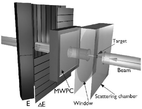
Figure 1: Schematic view of the detection system, presenting the relative positions of the MWPC, the two layers of the scintillation detectors and the scattering chamber containing the target. The central beam line transporting the primary beam to the target and further downstream to a distant Faraday cup is also indicated. For the sake of better view on the $E$-detector wall, 6 $\Delta E$ detectors (one sector) are removed from the figure.

The plastic scintillator hodoscope covered the range of polar angles between 10^∘ and 35^∘, and the full range of azimuthal angles. It consisted of 24 transmission detectors (horizontal $\Delta E$ strips) and 24 stopping detectors (vertical $E$ slabs), forming together a two-dimensional array of 140 elements, with an area of about 60$\times$60 mm² each. The system possessed mirror symmetries with respect to the horizontal and vertical planes, i.e. it could be viewed as composed of four similar sectors, each consisting of 6 slabs and 6 strips. Strips belonging to one sector formed telescopes with slabs of the same sector, while they had no overlap with slabs in other sectors. This physical grouping of detectors had a reflection in the trigger logic, based on combination of hit multiplicities within the sectors. Apart from trigger definition, information from the telescope array was used for particle identification and for determination of their energies.

The events of interest can be roughly divided into three classes. First we distinguish single events, for which only one $\Delta E$–$E$ telescope of the scintillation array has registered signals in a proper time window. The other two types are coincident events with two particles detected in two different telescopes. Among them a distinction was made between coincidences of elements belonging to the diagonal sectors (candidates for both, elastic scattering and breakup events) and elements of the adjacent sectors or belonging to the same sector (only breakup events). These three kinds of triggers were separately downscaled, enhancing the coincidence rates, to a level acceptable for the data acquisition system. Fine classification of events has been done off-line by incorporating the MWPC information – for an extensive description see MichPhD .

For each registered event the information from the readout system comprised data from the scintillator hodoscope and from the MWPC. The hodoscope data included times measured with respect to the cyclotron reference (rf) signal and pulse heights for all active detectors (strips and slabs). The MWPC information was coded into the numbers of the hit wires (more precisely – centers and widths of the adjacent groups, i.e. clusters, of wires). In addition, several auxiliary pieces of information were stored with each event: the beam polarization state, trigger pattern at various electronic stages, etc. Scalers, trigger rates, integrated beam current, pulse generator signals for dead-time monitoring, etc., were read out every 1 s.

II.2 Data analysis

All basic steps of the data analysis procedure, like event selection, energy calibration, determination of detection efficiencies and cross section normalization, have been thoroughly described in Kis03a . The description below recalls the main features with an emphasis put on the introduced improvements and on additional studies performed with the aim to reduce experimental uncertainties or to control their magnitude with enhanced accuracy.

II.2.1 Selection of events and background subtraction

The first step of the analysis was an adequate selection of the events of interest, i.e. coincident proton - proton pairs from the breakup process or, necessary for cross section normalization, deuteron - proton coincidences originating from the elastic scattering. To guarantee that only the products of the reactions initiated within a single beam burst were selected, a 20-ns-wide time window was imposed on the time spectra. Particle identification, based on the $\Delta E$–$E$ technique, proved to be very reliable, providing very good separation between protons and deuterons in the whole energy range.

Energy calibration was performed on the basis of data collected in special calibration runs with energy degraders of precisely known thicknesses. The positions of the peaks corresponding to protons from elastic scattering which traversed the degraders were compared with the results of simulations taking into account all energy losses of protons on their paths from the reaction point to the detectors. In this way the relation between ADC conversion (pulse height) and the energy deposited in the $E$ counter was found. The relation between the deposited energy and the proton energy at the moment of the reaction was obtained by analogous simulation of the proton energy losses. With all these provisions for each breakup event the initial energies of both protons ($E_{1}$ and $E_{2}$) were determined.

The coincidence (kinematic) spectra $E_{1}$ vs. $E_{2}$ were built for each analyzed configuration, defined by polar angles $\theta_{1}$, $\theta_{2}$ and relative azimuthal angle $\phi_{12}$ of the two emitted protons. The integration limits of $\Delta\theta_{1}=\Delta\theta_{2}=2^{\circ}$ and $\Delta\phi_{12}=10^{\circ}$ were used in all experimental integrations leading to the cross-section results, as well as in the studies concerning the performance of the detection system. The energies $E_{1}$ and $E_{2}$ of each event were transformed into two new variables: $D$, denoting the distance of the $(E_{1},E_{2})$ point from the kinematical curve in the $E_{1}-E_{2}$ plane, and $S$ – the value of the arclength along the kinematics. Events in slices along the $S$ axis were projected on the central $D$ axis, as shown in Fig. 2. In the resulting spectra (inset in Fig. 2), the breakup events group themselves in a prominent peak, underlaid with only a low background of accidental coincidences. As it has been already pointed out in Kis03a , the choice of integration limits $D_{\textrm{a}}$ and $D_{\textrm{b}}$, as well as of the assumed background function, is not critical since the contribution of accidental coincidences in all analyzed angular configurations was very low (between 2% and 5%). However, to treat all configurations in a consistent way, and since all the $D$-projected distributions have approximately Gaussian shape, the limits $D_{\textrm{a}}$ and $D_{\textrm{b}}$ were chosen at the values of $-3\sigma$ and $+3\sigma$ from the maximum of the fitted peak. A linear dependence of background between those points was assumed. Gaussian shape and linear background fitted to a sample distribution are shown in the inset of Fig. 2.

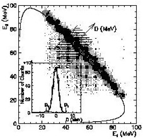
Figure 2: $E_{1}$ versus $E_{2}$ coincidence spectrum of the two protons registered at $\theta_{1}$ = 20${}^{\circ}\pm 1^{\circ}$, $\theta_{2}$ = 15${}^{\circ}\pm 1^{\circ}$ and $\phi_{12}$ = 100${}^{\circ}\pm 5^{\circ}$. The solid line shows a 3-body kinematical curve calculated for the central values of the experimental angular ranges. Inset: determination of the accidental coincidences. The spectrum was obtained by choosing one slice along the kinematical curve in the $E_{1}$ vs. $E_{2}$ spectrum (marked area in the main figure) and projecting the events onto the $D$ axis. Solid line represents the sum of a linear background function (shown with the dashed line) and a Gaussian distribution, fitted in the range of $D$ between $D_{\textrm{a}}$ and $D_{\textrm{b}}$, corresponding to distances of $-3\sigma$ and $+3\sigma$ from the peak position.

II.2.2 Detection efficiency

The efficiency in determining the particle-emission angles, called for simplicity the MWPC efficiency, is a product of hardware efficiencies of the MWPC wire planes and the efficiency of our procedure of reconstructing the angles. Since we accepted only events with vertical and horizontal wires properly correlated with the corresponding $E$ and $\Delta E$ detectors, the ranges of wire numbers associated with the individual hodoscope elements had to be set wide enough. These correlation tables were revised once again (with respect to the procedure of Ref. Kis03a ), inspecting the whole data sample and the ranges of wires associated with each hodoscope element have been slightly broadened. In this way, since there was practically no uncorrelated noise on the wires, no additional background was introduced while the efficiency was increased. With these new conditions the efficiency has been recalculated in the manner similar to the one described in Kis03a and, in addition, losses due to the requirement of correlation between all three planes have been determined. In spite of imposing this last restriction with reasonable “safety limits” of $\pm 3$ wires in $u$ plane, some protons scattered on their way to MWPC escaped those limits and were rejected, affecting the total efficiency. The final map of the MWPC efficiency is presented in Fig. 3.

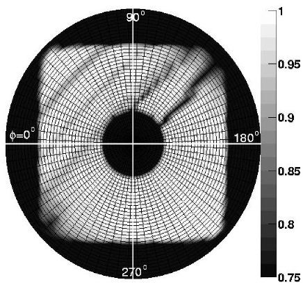
Figure 3: Global efficiency map for the MWPC, presented as a polar plot in the angular coordinates. Only the square-like area of the map is meaningful. The range of polar angle $\theta$ is from 0^∘ to 40^∘ with the binning of 1^∘ and the azimuthal angle $\phi$ covers the full range with the binning of 5^∘. The discontinuities of lower efficiency regions are the result of this finite binning.

Thorough studies of the detection and trigger efficiencies were supplemented with additional tests, performed for configurations with the relative azimuthal angle of the two protons exceeding 90^∘. Such configurations can be realized by two mutually exclusive classes of events: when the two protons were registered in either the adjacent sectors or in two diagonal sectors of the hodoscope. These two cases corresponded to different trigger signals and different downscaling factors, therefore any relative inefficiency of the trigger logic and/or of the downscaling should be reflected by influencing the relative amount of events of the two groups. It should be stressed that we are sensitive only to the relative efficiency of the two trigger classes: since the events originating in the elastic scattering are always registered in diagonal sectors, the trigger/detection efficiency for the diagonal sectors cancels out in normalization, cf. Eq. (1). Each of the two event groups was analyzed separately and the ratio of their rates as a function of the arclength $S$ was constructed. An analogous ratio was calculated for simulated events. For all the configurations the experimental ratio is constant along $S$ and agrees with the result of simulations within statistical accuracy of 0.8% or less, depending on the configuration (see example in Fig. 4). The above result confirms not only the correct functioning of the trigger but also proper handling of the detection efficiencies in the analysis.

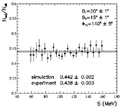
Figure 4: Ratio of event rate of proton-proton coincidences registered in two adjacent sectors to the total rate of events (adjacent + diagonal) for configuration $\theta_{1}=20^{\circ}\pm 1^{\circ}$, $\theta_{2}=15^{\circ}\pm 1^{\circ}$, $\phi_{12}=140^{\circ}\pm 5^{\circ}$. Points represent experimental values obtained by integrating the events within the given bin of the arclength $S$. Solid line shows the level fitted to the data, the dashed one the ratio obtained from the simulation. Numerical results with statistical errors are given for both, experimental and simulated data.

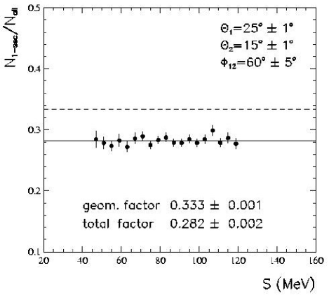
Figure 5: Ratio of the rate of single-sector events to the total rate of events (one-sector plus two-sector) for configuration $\theta_{1}=25^{\circ}\pm 1^{\circ}$, $\theta_{2}=15^{\circ}\pm 1^{\circ}$, $\phi_{12}=60^{\circ}\pm 5^{\circ}$. Points show the experimental values obtained within 4 MeV $S$-bins. The difference between the purely geometrical factor (dashed line) and the total correction factor (solid line) including the acceptance losses for single-sector events, is clearly visible. Numerical values of the factors are given with their statistical uncertainties.

In configurations with the relative azimuthal angle of two protons $\phi_{12}$ not exceeding 90^∘ additional losses of acceptance have to be taken into account, due to cases when both protons were registered in the same $\Delta E$ or $E$ detector (impossible proper particle identification and/or energy determination), or in two adjacent $E$ detectors. In the latter case, if at least one of the two protons was registered close to the edge of the two $E$ detectors, the event cannot be distinguished from a so-called cross-over and had to be rejected (cf. Sec. II.2.3). Obviously, only single-sector events are affected by these effects. Therefore, the total correction factor is obtained as a product of the ratio of events with both protons emitted into a single sector to all events collected in the specific configuration, and the actual correction, describing the losses within the single sector. Experimentally, the total correction can be determined by the ratio of the breakup events registered in single sectors to all events of the considered configuration. By means of simulation one can investigate both contributions separately. First, in order to find for each configuration with $\phi_{12}<100^{\circ}$ purely geometrical factors of probability for single-sector events, an ideal case was assumed with no losses due to the detector granularity. Then, the events were artificially digitized and analyzed in the same way as the experimental ones. It has been found that the acceptance losses reduce the geometrical factors by up to 13%, depending on the configuration, but they are constant as a function of $S$ for the selected geometry. In Fig. 5 an example comparing the pure geometrical and the total correction factors is shown for one configuration. In general the losses increase with decreasing relative azimuthal angle and with the increasing difference of the polar angles. It should be noted that the errors introduced by applying the correction factors are much smaller than the factors themselves.

II.2.3 Cross-over correction

The procedure of energy calibration faces a problem in determining the energy of particles which penetrate from one stopping detector to the adjacent one, in the so called cross-over events. Simple summing up of the two deposited energies is not completely adequate due to energy losses in the foil covering all the detector walls. Additionally, in a particular situation when the energy deposited in one of the $E$ slabs is below the detection threshold, the energy information is significantly distorted and, moreover, there is even no obvious signature of cross-over. Such events are shifted away from the kinematic curve and contribute to the background attributed to accidental coincidences, which is then subtracted in the way described in Section II.2.1.

Therefore, a new approach was used, in which all cross-over candidates were rejected from the analysis (in a way explained below) and their amount was determined with the use of Monte-Carlo simulation based on the GEANT4 package. Narrow regions corresponding to the detector borders were defined with the help of high-resolution MWPC position coordinates and the particles which entered those regions and induced signals in two adjacent $E$ detectors were discarded. Treating the simulated data in the same way it was possible to find the ratio of rejected to registered event numbers for every configuration, which was used to correct the experimental rates. The simulations were performed for elastic scattering and for all studied configurations of the breakup reaction. For elastic scattering, due to rather high proton energy and constrained kinematics the effects are quite large – on average about 7% of all the events is biased with the cross-over possibility. The corresponding correction factors vary strongly, from 4% to 11%, depending on the proton polar angle $\theta_{p}$. Their impact is demonstrated by the fact that application of this correction leads to the experimental cross-section distribution for elastic scattering (Fig. 6) with a smoother dependence on $\theta_{p}$, following more closely the reference $pd$ data. It is also reflected by a decrease of the $\chi^{2}$ value calculated between the two distributions by a factor of about 2 with respect to the result obtained for the uncorrected data. Contributions of the cross-over events, calculated individually for each analyzed configuration of the breakup reaction, vary between 2% and 5%. The individual cross-over correction factors were applied when evaluating the differential breakup cross sections, resulting in a decrease of their systematic uncertainty.

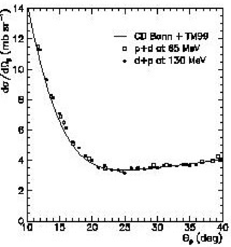
Figure 6: Experimental angular distribution of the elastic scattering events. The absolute normalization of our data (full circles) is adjusted to best fit the reference data. Statistical errors are smaller than the point size. Empty squares represent the reference cross-section values Shi82a . Solid line shows the results of the theoretical calculations obtained with the CD Bonn potential and the TM99 3NF model.

II.2.4 Cross section normalization

The breakup cross sections are normalized to the elastic scattering one, using the measured in parallel rates of the elastic scattering events and the available $pd$ elastic scattering cross-section data. The differential breakup cross section for a chosen angular configuration is thus expressed in terms of the elastic scattering cross section and both measured coincidence rates:

$$\frac{d^{5}\sigma}{d\Omega_{1}d\Omega_{2}dS}(S,\Omega_{1},\Omega_{2})=\frac{d\sigma_{el}}{d\Omega_{1}^{el}}(\Omega_{1}^{el})\cdot\frac{N_{br}(S,\Omega_{1},\Omega_{2})}{N_{el}(\Omega_{1}^{el})}\times$$

$$\times\>\frac{\Delta\Omega_{1}^{el}}{\Delta\Omega_{1}\Delta\Omega_{2}\Delta S}\cdot\frac{\epsilon^{el}(\Omega_{1}^{el})\epsilon^{el}(\Omega_{2}^{el})}{\epsilon(\Omega_{1})\epsilon(\Omega_{2})}\;,\;\,$$ (1)

where $N_{br}$ is the number of breakup coincidences registered at the angles $\Omega_{1}$, $\Omega_{2}$ and projected onto a $\Delta S$-wide arclength bin. Subscripts 1 and 2 refer to the first and the second proton registered in coincidence or to the proton and the deuteron in the case of elastic scattering. $\Omega_{i}\equiv(\theta_{i},\phi_{i})$, with $i=1,2$, are the polar and azimuthal angles, respectively, and $\Delta\Omega_{i}$ is the solid angle ($\Delta\Omega_{i}=\Delta\theta_{i}\Delta\phi_{i}\sin{\theta_{i}}$). Products $\epsilon(\Omega_{1})\epsilon(\Omega_{2})$ (or $\epsilon^{el}(\Omega_{1}^{el})\epsilon^{el}(\Omega_{2}^{el})$) contain all relevant efficiencies and correction factors (cf. Sec. II.2.3). $N_{el}$ is the final number of elastic scattering $pd$ coincidences registered at the proton angle $\Omega_{1}^{el}$. The elastic scattering cross section $\frac{d\sigma_{el}}{d\Omega_{1}^{el}}(\Omega_{1}^{el})$ is taken from Shi82a . The bin width $\Delta S$ was chosen to be 4 MeV.

In such an approach we profit from cancellation of all factors related to the luminosity, i.e. the integrated beam current, the density and the thickness of the target. Moreover, since events from both reactions are processed by common electronic and read-out systems, the relevant dead-time corrections cancel out in the ratio of the registered events. In that way factors which would be difficult to determine individually and would induce systematic uncertainties are greatly eliminated.

II.2.5 Experimental uncertainties

A full discussion of the experimental uncertainties has been presented in Kis03a . The statistical accuracy comprises the error of the measured number of the breakup coincidences, as well as statistical uncertainties of all quantities used in the cross-section normalization, i.e. the number of the elastic scattering events and all efficiencies included in Eq. (1). Taking into account the range of the cross-section values for our data points, the magnitude of the statistical errors varies between 0.5% and 4.0%.

Non-negligible systematic effects can originate from the cross section normalization, from uncertainty of the energy calibration parameters, from incomplete cancellation of polarization effects in the cross section (1.0%) and from the procedure of reconstruction of the proton emission angles. By introducing the cross-over corrections we were able to suppress variations in the experimentally obtained elastic scattering distribution and therefore reduce the total uncertainty of the normalization procedure down to about 2.0%. The uncertainty of the energy calibration can result in changing the length of the experimental distribution along the $S$-curve by at most 0.7%. The relative cross-section errors resulting from such change vary between 0.7% and 2.5%, for central and peripheral regions of the measured $S$-ranges. This is the only systematic uncertainty which changes along the arclength $S$ in every configuration; all other contributions are rather configuration-specific.

The uncertainty of the reconstructed value of the angle is due mainly to finite target thickness, finite size of the beam spot on the target, straggling effects and angular resolution related to the discreteness of the position information delivered by the MWPC. The well-reproduced correlation of the proton and deuteron emission angles for elastic $dp$ scattering confirms that there is no (at the level below 0.3^∘) systematic shift of the reconstructed polar angles. The other effects, resulting in smearing out of the angular resolution, have been studied by the dedicated simulation, based again on the GEANT4 package. In order to reproduce conditions of the real measurement, realistic distribution of the reaction vertices and theoretical angular dependence of the breakup cross section were assumed. Straggling effects in materials were introduced by means of GEANT4 transport routines and, finally, the positions of proton trajectories intersecting the wire planes were translated to hits on the wires. The same reconstruction algorithm as for the real data was applied to the simulated events. In this way we were able to compare the amount of events in each configuration defined by proton emission angles, with the number of events in the same configurations, but defined with the use of the reconstructed angles. It was found that for about 30% of events selected on the basis of the reconstructed angles the particles were really emitted at angles lying outside the chosen angular range. On the other hand, practically the same amount of events emitted into the chosen range is reconstructed with the values of angles not belonging to the considered configuration, and therefore rejected. In this way the number of events in “true” and “reconstructed” configurations is very well balanced: differences are between 0.2% and 1.0% and do not contribute significantly to the cross section errors.

Table 1: Summary of the relevant experimental cross-section uncertainties. Two sample cross-section data points (with values close to the minimal and maximal ones measured) are selected for presenting individual contributions to the systematic uncertainties:
(1) $\theta_{1}=\theta_{2}=15^{\circ}$, $\phi_{12}=60^{\circ}$, $S$ = 106 MeV,
      d${}^{5}\sigma$/d$\Omega_{1}$d$\Omega_{2}$d$S$ = 0.078 mb$\cdot$sr${}^{-2}\cdot$MeV^-1,
(2) $\theta_{1}=\theta_{2}=25^{\circ}$, $\phi_{12}=160^{\circ}$, $S$ = 134 MeV,
      d${}^{5}\sigma$/d$\Omega_{1}$d$\Omega_{2}$d$S$ = 1.57 mb$\cdot$sr${}^{-2}\cdot$MeV^-1.
The last column shows all the overall ranges of the relative cross section uncertainties. The “total systematic” error is obtained by adding the squares of all the contributions.

	$\delta\sigma_{1}$	$\delta\sigma_{2}$	$\delta\sigma$ range
Source of uncertainty	(%)	(%)	(%)
Statistical	2.7	0.6	0.5 – 4.0
Energy calibration	1.9	0.7	0.7 – 2.5
Beam polarization	1.0	1.0	1.0
Reconstruction of angles	0.6	0.5	0.2 – 1.0
Choice of integration region	0.3	0.1	0.1 – 1.0
Normalization:	1.6	2.0	1.6 – 2.0
Total systematic	2.8	2.4	2.0 – 3.6

The complete simulation of the breakup process lead to the conclusion that the influence of angular resolution on the cross section is in fact smaller than what was found from the geometrical estimations Kis03a . Including all improvements of the current analysis, the total systematic uncertainty is lower by about 1% as compared to the previously quoted values. The experimental uncertainties relevant for the cross sections presented here are summarized in Table 1. The overall ranges of uncertainties (last column) are not to be associated with particular magnitudes of the cross sections. An obvious exception is apparently the statistical accuracy; however, since data were collected with different downscaling factors and there are certain acceptance losses, this scaling is also not straightforward. Therefore, we have selected two cross-section points with values close to the minimal and maximal of all presented in Sec. IV and we display for them the individually calculated contributions to their uncertainties. One can observe that uncertainties of the larger measured cross sections are usually dominated by systematic effects, while for the smaller values of cross sections the contributions from systematic and statistical errors are comparable.

III Theoretical Formalism

III.1 Realistic potentials

The calculation of the cross-section values using realistic potentials is performed exactly as outlined in our previous study Kis03a , following our standard method for the 3$N$ continuum. The general overviews of our formulation of the 3$N$ scattering problem and of including 3NF into the scheme are given in Glo96a and Hub97a , respectively. In the following a very brief review is presented.

We use the modern, realistic $NN$ potentials AV18 AV18 , charge dependent (CD) Bonn CDBonn1 ; CDBonn2 , and Nijm I and II NijmIII . Investigating the full 3$N$ system dynamics, we combine them with the 2$\pi$-exchange TM 3NF, taking its recent form TM993NF , consistent with chiral symmetry, which will be denoted by TM99. The TM99 3NF model contains one parameter, $\Lambda_{TM}$, used as cut-off to regularize its high-momentum behavior. The value of $\Lambda_{TM}$ is adjusted for each particular combination of the $NN$ force and the TM99 3NF to match the value of the ³H binding energy Nog97a . For the four 2$N$ potentials used in the calculations the corresponding values of $\Lambda_{TM}$ (in units of the pion mass $m_{\pi}$) are 4.764, 4.469, 4.690 and 4.704, respectively.

When the 3$N$ system dynamics is studied with the AV18 $NN$ potential, we combine it also with the Urbana IX 3NF UIX3NF (UIX). To apply it within our framework it was necessary to transform its configuration-space form to momentum space Wit01a .

Having the $NN$ and 3$N$ forces, the scattering problem in the 3$N$ system is stated in form of a Faddeev-like integral equation for an amplitude $T$:

$$T = t\,P\,\phi\ +\ (1+tG_{0})\,V_{3NF}^{[1]}\,(1+P)\,\phi\ +\ t\,P\,G_{0}\,T$$ (2)

$$\mbox{}+\ (1+tG_{0})\,V_{3NF}^{[1]}\,(1+P)\,G_{0}\,T\,,$$

where the initial channel state $\phi$ is composed of a deuteron and a momentum eigenstate of the projectile nucleon. The $NN$ transition operator is denoted by $t$, the free 3$N$ propagator by $G_{0}$ and $P$ is the sum of a cyclical and an anti-cyclical permutation of the three particles. The 3$N$ potential $V_{3NF}$ can always be decomposed into a sum of three parts:

$$V_{3NF}=V_{3NF}^{[1]}+V_{3NF}^{[2]}+V_{3NF}^{[3]}\,,$$ (3)

where the part $V_{3NF}^{[i]}$ singles out nucleon $i$, on which the pion is rescattered. The parts are symmetric under the exchange of the two nucleons $j$ and $k$, with $j\neq i\neq k$. One can see that in Eq. (2) only one part, $V_{3NF}^{[1]}$ appears explicitly; the others enter via the permutations contained in $P$. The physical breakup amplitude $U_{0}$ is obtained from $T$ by

$$U_{0}=(1+P)T\,.$$ (4)

Iterating the Faddeev-like equation (2) and inserting the resulting $T$ into Eq. (4) yields the multiple scattering series, in which each term contains some number of interactions among nucleons via 2$N$- and 3$N$-forces with free propagation in between. The reaction mechanism is thus transparently mirrored.

We solve Eq. (2) using a momentum space partial-wave basis Glo96a . To guarantee converged solutions for our case of 130 MeV incoming deuterons we take into account all partial waves with $j_{max}<6$ in the 2$N$ subsystem. This gives rise to the maximal number of 142 partial wave states in the 3$N$ system for each total 3$N$ angular momentum $J$. The convergence has been checked by inspecting the results obtained for $j_{max}=6$ calculations without a 3NF (total number of channels increased to 194). Finally, the breakup amplitudes $U_{0}$ have been calculated for all total angular momenta of the 3$N$ system up to $J=25/2$ for any $NN$ interaction, while the inclusion of 3NF’s has been carried out for all states up to $J=13/2$. From this amplitude the cross section is obtained in a standard manner Glo96a .

III.2 Chiral Perturbation Theory

The chiral 2$N$ potential at the next-to-next-to-leading order (NNLO) used in the present study is derived from the most general effective chiral Lagrangian, based on the method of unitary transformation Epe98a and using the spectral function regularization (SFR) Epe05a . More details about the employed regularization schemes and the corresponding cut–offs can be found in Epe05a . Completing the 3$N$ system dynamics at NNLO with the naturally and consistently arising 3NF contributions is presented in Epe02a . We recall below a few key features.

The 2$N$ force is obtained by summing up contributions from graphs of increasing complexity, accounting for, roughly speaking, two kinds of processes: long range pion(s) exchanges, where chiral symmetry plays a crucial role and short range phenomena, which are effectively treated by means of $NN$ contact interactions. The corresponding low energy constants (LEC’s) are determined from the $NN$ data. The potential is expressed in terms of the expansion in powers $\nu$ of $Q/\Lambda_{\chi}$, where $Q$ is the soft scale, corresponding to the nucleon external momenta and the pion mass and $\Lambda_{\chi}$ is the hard scale (around 1 GeV) associated with the chiral symmetry breaking scale or the ultraviolet cut–off(s). For each diagram contributing to the potential, the power $\nu$ can be calculated according to the power counting scheme Wei90a , see also Epe98a .

Up to NNLO, the chiral $NN$ potential can be written as

$$V^{NN}=V^{(0)}+V^{(2)}+V^{(3)}\,.$$ (5)

At the leading order (LO, $\nu$ = 0) the $NN$ potential $V^{(0)}$ is given by the one-pion exchange part (1PE) and two contact interactions:

$$V^{(0)}=V_{1\pi}^{(0)}+V_{cont}^{(0)}\,.$$ (6)

The leading 1PE term is expressed in terms of standard constants: the pion decay constant $F_{\pi}$, the pion mass $m_{\pi}$ and the axial-vector nucleon coupling $g_{A}$. In the contact term two LEC’s are introduced, $C_{S}$ and $C_{T}$. The next-to-leading order (NLO, $\nu$ = 2) corrections are due to two-pion exchanges (2PE), seven new contact interactions and a correction to 1PE:

$$V^{(2)}=V_{2\pi}^{(2)}+V_{1\pi}^{(2)}+V_{cont}^{(2)}\,.$$ (7)

The leading 2PE term introduces no new parameters (except the SFR cut-off, see below), the contact terms are characterized by seven constants $C_{1},...,C_{7}$ and in the 1PE correction term the constant $d_{18}$ can be incorporated by renormalization of $g_{A}$ – see Epe05a ; Epe03a for more details. Finally, the NNLO ($\nu$ = 3) corrections are given by the subleading 2PE potential and corrections to the 1PE force:

$$V^{(3)}=V_{2\pi}^{(3)}+V_{1\pi}^{(3)}\,;$$ (8)

there are no new contact terms. The 2PE term contains three new LEC’s, $c_{1}$, $c_{3}$ and $c_{4}$. The LEC’s $C_{S}$, $C_{T}$ and $C_{1},\ldots,C_{7}$, appearing at LO and NLO, are obtained by fitting the $V^{NN}$ predictions to the $NN$ data (more precisely, to the lowest phase shifts). The three LEC’s $c_{1}$, $c_{3}$ and $c_{4}$ entering the 2PE contribution at NNLO can be determined from the $\pi N$ scattering data. It has been shown Epe04a that the adopted values lead to a proper reproduction of the deuteron properties and of the phase-shift analysis results.

A non-vanishing chiral 3NF arises only at NNLO (in the energy-independent formulation) and can be written as

$$V^{3NF}=V^{3NF}_{2\pi}+V^{3NF}_{1\pi}+V^{3NF}_{cont}\,.$$ (9)

The three terms account for three different topologies Epe02a . The $V^{3NF}_{2\pi}$ describes a simultaneous exchange of two pions and incorporates the same LEC’s $c_{1,3,4}$ as in the subleading 2PE $NN$ potential $V_{2\pi}^{(3)}$. The $V^{3NF}_{1\pi}$ contribution arises due to a single pion being exchanged between a nucleon and a 2$N$ contact interaction. The contact term contains one parameter, which is usually called $c_{D}$. Finally, the $V^{3NF}_{cont}$ describes a contact interaction of three nucleons and introduces another LEC, labeled $c_{E}$. These two last LEC’s are fixed by the requirement to reproduce the ³H binding energy and the $nd$ doublet scattering length – see Epe02a for a detailed discussion.

In representing the chiral potential we use the spectral function decomposition Epe04a and we reject the large-mass (momentum) fraction of the 2PE via a step Heaviside function with the cut-off parameter $\tilde{\Lambda}$. In the 2PE contributions at NLO and NNLO the loop functions are thus regularized and the corresponding short-distance phenomena are shifted into the contact terms (the LEC’s are appropriately adjusted). This procedure, called SFR, possesses numerous advantages over formerly implemented dimensional regularization Epe04a ; Epe05a . Its implementation allowed us also to use LEC’s $c_{1,3,4}$ consistent with the $\pi N$ data, in contrast to the former study Epe02a , where the 3$N$ dynamics was described in a so-called NNLO* approach, with artificially small values of these constants.

Using the resulting potential, the $t$-matrix is obtained via numerical, non-perturbative solution of the partial-wave projected Lippmann-Schwinger (LS) equation. Since the effective 2$N$ forces are meaningless for large momenta, we still have to reject contributions of the high-momentum states. In this way we also avoid an ultraviolet divergence of the LS equation. The standard procedure to accomplish those requirements is to regularize the potential by multiplying it with a regulator function, containing an additional cut-off parameter $\Lambda$. As in other studies Epe04a ; Epe05a , we use a Gaussian regulator function. The $T$ operator of the 3$N$ scattering problem is obtained in an identical way as for realistic potentials (cf. Sec. II.1), by solving the Faddeev-like equation (Eq. 2) with the chiral 3NF from Eq. (9). To keep the treatment of 2$N$ and 3$N$ interactions consistent, we use an appropriate regulator function with the same cut-off parameter $\Lambda$ as for the $NN$ potential in the LS equation also for regularization of the chiral 3NF. In further calculations the observables are generated on the basis of the obtained breakup amplitude $U_{0}$.

Our method provides the possibility to estimate uncertainties of the calculated predictions. We perform calculations with a few combinations of the two cut-off parameters, [$\Lambda$,$\tilde{\Lambda}$]. The range of predictions obtained for reasonable choice of the variation intervals of both cut-offs gives an estimate of the theoretical uncertainty. For details on how one selects the proper ranges of regularization cut-off values we refer to Epe04a ; Epe05a and references therein. In the present study we use the following pairs of the cut-off parameters (values in MeV):

$$[\Lambda,\tilde{\Lambda}] = [450,500],[600,500],[550,600],$$ (10)

$$[450,700],[600,700]\,.$$

III.3 Coupled-channel potential

A new realistic two-baryon potential coupling $NN$ and $N\Delta$ states has been presented in detail in Del03b , with several examples of its application to calculate observables for the 3$N$ system. The main features of this approach are briefly recalled here.

The dynamics of the 3$N$ system is described with the explicit treatment of the $\Delta$-isobar excitation, considered in the relevant energy range as a stable particle. The three nucleon channels are coupled to those in which one nucleon is excited and forms the $\Delta$-isobar. Creation of a virtual excited state yields an effective 3NF, in parallel to other aspects of the dynamics induced by the $\Delta$-isobar.

The method for extending a model of $NN$ interaction to include $\Delta$-isobar degrees of freedom has been worked out in Haj83a and recently thoroughly upgraded Del03b , taking the purely nucleonic CD Bonn potential CDBonn2 as a reference. Such a coupled-channel potential is based on the exchange of $\pi$, $\rho$, $\omega$, and $\sigma$ mesons, and in addition to the purely nucleonic part includes also contributions from the transition between the $NN$ and $N\Delta$ states, from the exchange $N\Delta-\Delta N$ potential and from the direct interaction of the $N\Delta$ states. The force employed here, referred to as CD Bonn + $\Delta$, is as realistic as any of the $NN$ force models quoted in Sections I and III.1, reproducing the data of the 2$N$ system with a $\chi^{2}$ per degree of freedom of 1.02 Del03b . It is purely nucleonic in the isospin singlet states; the coupled-channel two-baryon extension acts in isospin triplet states only, where a few constants of the reference $NN$ force are retuned. Prominent contributions of the effective 3NF mediated by the $\Delta$-isobar are of the Fujita-Miyazawa type FM3NF and of the Illinois ring type Pie01a . The contributions are based on all meson exchanges, i.e. $\pi$, $\rho$, $\sigma$ and $\omega$ exchanges, contained in the coupled-channel potential; the $\Delta$ propagation is retarded. The arising effective three-nucleon force is much richer with respect to the $\Delta$ excitation and also has shorter ranged components than standard irreducible two-pion exchange 3NF’s. Furthermore, all its components are dynamically consistent with each other and with the effective 2$N$ force. However, in addition to the $\Delta$-mediated 3NF an irreducible 3NF covering other physics mechanisms is not used.

The solution of the three-baryon scattering problem is based on the AGS equation formulation, using a Chebyshev expansion of the two-baryon transition matrix as the interpolation technique Del03a . The multichannel transition matrix $U$ between two-body channels is obtained from:

$$U=P\,G_{0}^{-1}+P\,T_{\alpha}\,G_{0}\,U\,,$$ (11)

where $T_{\alpha}$ is the two-baryon transition matrix in three-baryon space (the subscript $\alpha$ denoting the pair $\beta$-$\gamma$ of interacting baryons, $\alpha\neq\beta\neq\gamma$), $G_{0}$ is the free resolvent $(E-i0-H_{0})^{-1}$ with the total available energy $E$ and free Hamiltonian $H_{0}$, and $P$ is the permutation operator introduced in Eq. (2). The transition matrix $T_{\alpha}$ results from the full form of the two-baryon potential $V_{\alpha}$, acting between baryons $\beta$ and $\gamma$:

$$T_{\alpha}=V_{\alpha}+V_{\alpha}\,G_{0}\,T_{\alpha}\,.$$ (12)

The breakup transition matrix $U_{0}$ is obtained from $U$ according to

$$U_{0}=(1+P)\,G_{0}^{-1}+(1+P)\,T_{\alpha}\,G_{0}\,U\,.$$ (13)

The first term on the right side of Eq. (13) does not contribute to the on-shell matrix elements of $U_{0}$, needed to calculate breakup observables. The approach described here is very similar to the one outlined in Sec. III.1. If we define the amplitude $T$ as:

$$T=T_{\alpha}\,G_{0}\,U\,,$$ (14)

then the integral AGS equation (11) after simple algebra becomes identical with the Faddeev-like equation (2), in which the 3NF potential is set to zero and the $NN$ $t$-operator is identified with $T_{\alpha}$. Following the remark below Eq. (13), that equation becomes immediately identical with Eq. (4).

Matrix elements of the amplitudes $U$ and $T$, necessary to calculate breakup observables, are found in the partial-wave basis. The charge dependence of the two-baryon potential is treated as described in Del03b , yielding the total isospin $\frac{3}{2}$ channels in the ${}^{1}S_{0}$ state. In the purely nucleonic channels all the states with $j_{max}<6$ in the two-baryon system have been taken into account, while for the $N\Delta$ channels the applied total angular momentum limitation was $j_{max}<5$. In the full three-baryon space the states with angular momentum up to $J_{max}=31/2$ were taken into account. For the energy considered here, the results are fully convergent with respect to both, $j_{max}$ and $J_{max}$ limitations, what was tested by checking several predictions obtained with the limits $j_{max}=6$ and $J_{max}=35/2$.

The discussion of the coupled-channel potential approach should be closed with a few remarks. The mechanism of explicit $\Delta$ excitation in the three-baryon interaction has two distinct effects: it yields an effective repulsive potential (two-baryon dispersion) and it induces an effective 3NF. These two contributions usually compete Del03b ; Del03c , resulting in relatively modest differences when comparing the results of CD Bonn and CD Bonn + $\Delta$ predictions. The competition might be less pronounced at higher energies. It should be also noted that in this method the binding energies of the 3$N$ systems are reproduced a bit less perfectly than in the other approaches. On the other hand, only in this framework has a significant development towards including the Coulomb interaction into the Faddeev formalism for the 3$N$ continuum been achieved recently Del05a .

IV Results

The main purpose of this paper is a systematic study of the quality by which the breakup cross sections can be reproduced by theoretical predictions. The investigation spans a significant fraction of the breakup reaction phase space, the attainable geometries defined by our experimental conditions. In our methodical approach of scanning the phase space we present the cross-section data for a regular grid of polar and azimuthal angles with a constant step in the arclength variable $S$. Polar angles of the two protons $\theta_{1}$ and $\theta_{2}$ are changed between 15^∘ and 30^∘ with the step size of 5^∘ and their relative azimuthal angle $\phi_{12}$ is analyzed in the range from 40^∘ to 180^∘, with the step size of 20^∘. We are able to extract data covering a denser grid. However, since the changes of the breakup cross section are rather smooth, already this coverage allows to draw all the important conclusions. For each combination of the central values $\theta_{1}$, $\theta_{2}$ and $\phi_{12}$ the experimental data were integrated (cf. Sec. II.2.1) within the limits of $\pm$ 1^∘ for the polar angles and of $\pm$ 5^∘ for the relative azimuthal angle. The bin size along the kinematic curve $S$ was 4 MeV. Such limits allowed us to reach sufficient statistical accuracy while keeping the angle and energy integration effects to a minimum, not affecting the comparison with the point-geometry theoretical predictions (see below).

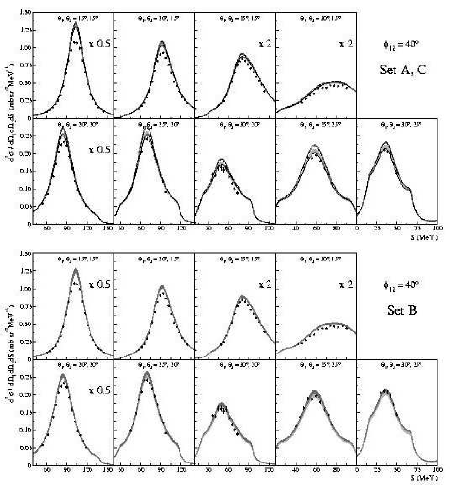
Figure 7: Experimental breakup cross sections in 9 kinematical configurations for the relative azimuthal angle of the two protons $\phi_{12}$ = 40^∘ and for various combinations of the proton polar angles, as indicated in the individual panels. The error bars represent statistical uncertainties only. In a few panels the results are scaled with the indicated scaling factors to fit the common vertical axis. Upper part: data compared to predictions obtained with the realistic $NN$ potentials only (light-shaded bands), with calculations of the pairwise $NN$ forces combined with the TM99 3NF (dark-shaded bands) and of AV18 + Urbana IX (dashed lines). The solid line represents the results obtained for calculations within the coupled-channel framework with the CD Bonn + $\Delta$ potential. Lower part: the same data confronted with the predictions obtained within the ChPT approach at NNLO. The complete calculations are represented by the dark-shaded bands, while the light-shaded ones demonstrate the results with the dynamics constrained to only $NN$ contributions.

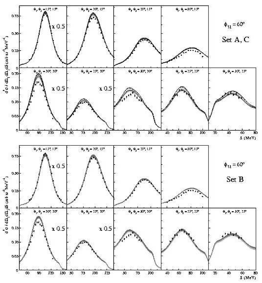
Figure 8: The same as in Fig. 7 but for kinematic configurations with the relative azimuthal angle of two protons $\phi_{12}$ = 60^∘.

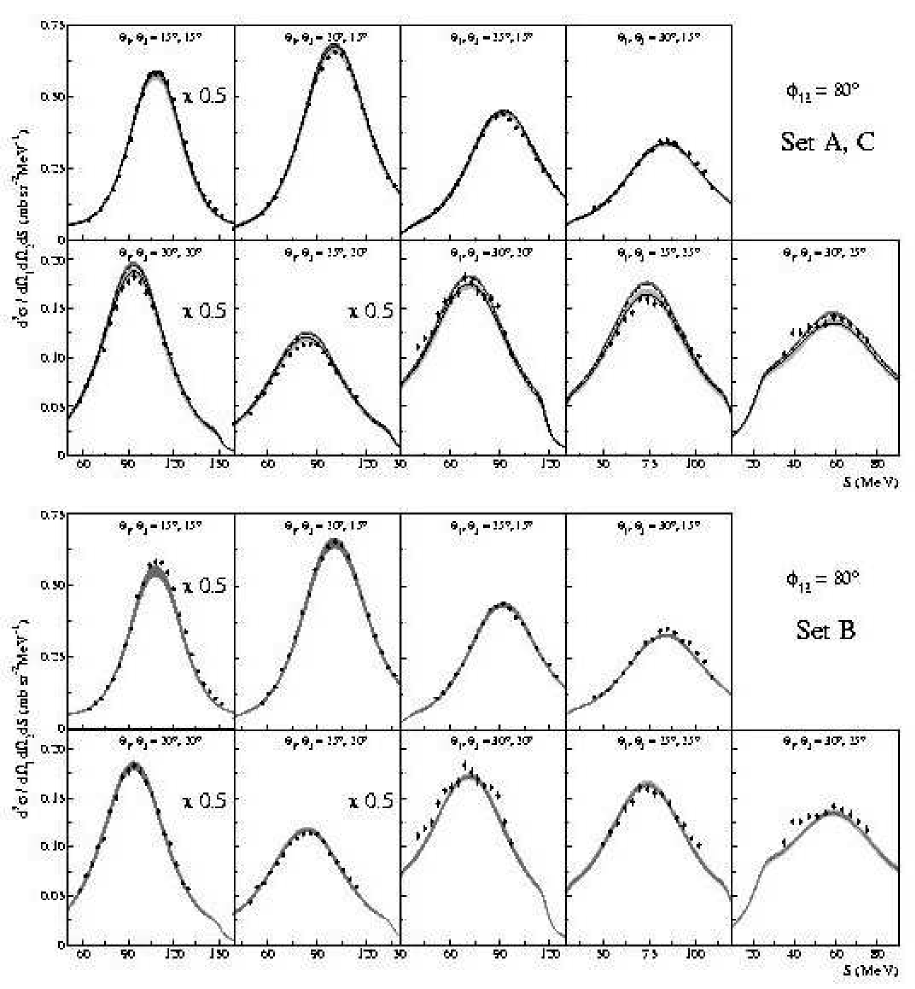
Figure 9: The same as in Fig. 7 but for kinematic configurations with the relative azimuthal angle of two protons $\phi_{12}$ = 80^∘.

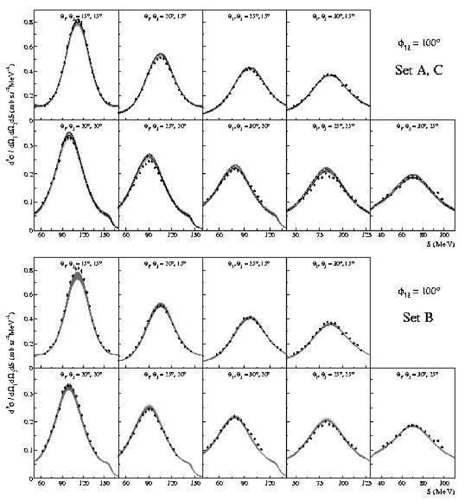
Figure 10: The same as in Fig. 7 but for kinematic configurations with the relative azimuthal angle of two protons $\phi_{12}$ = 100^∘.

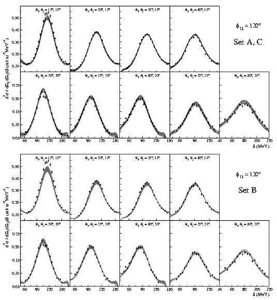
Figure 11: The same as in Fig. 7 but for kinematic configurations with the relative azimuthal angle of two protons $\phi_{12}$ = 120^∘.

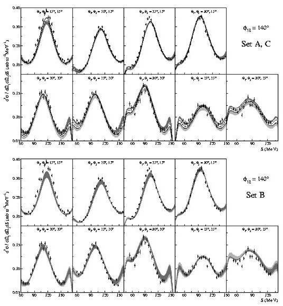
Figure 12: The same as in Fig. 7 but for kinematic configurations with the relative azimuthal angle of two protons $\phi_{12}$ = 140^∘.

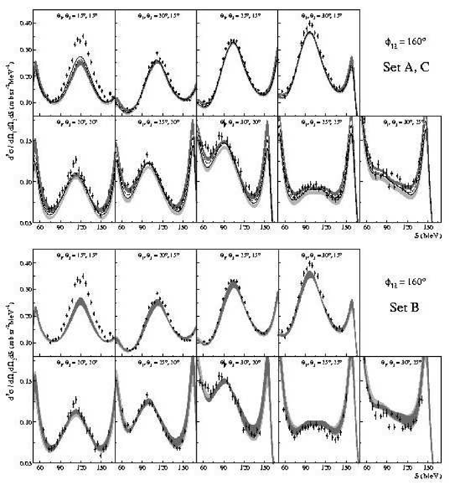
Figure 13: The same as in Fig. 7 but for kinematic configurations with the relative azimuthal angle of two protons $\phi_{12}$ = 160^∘.

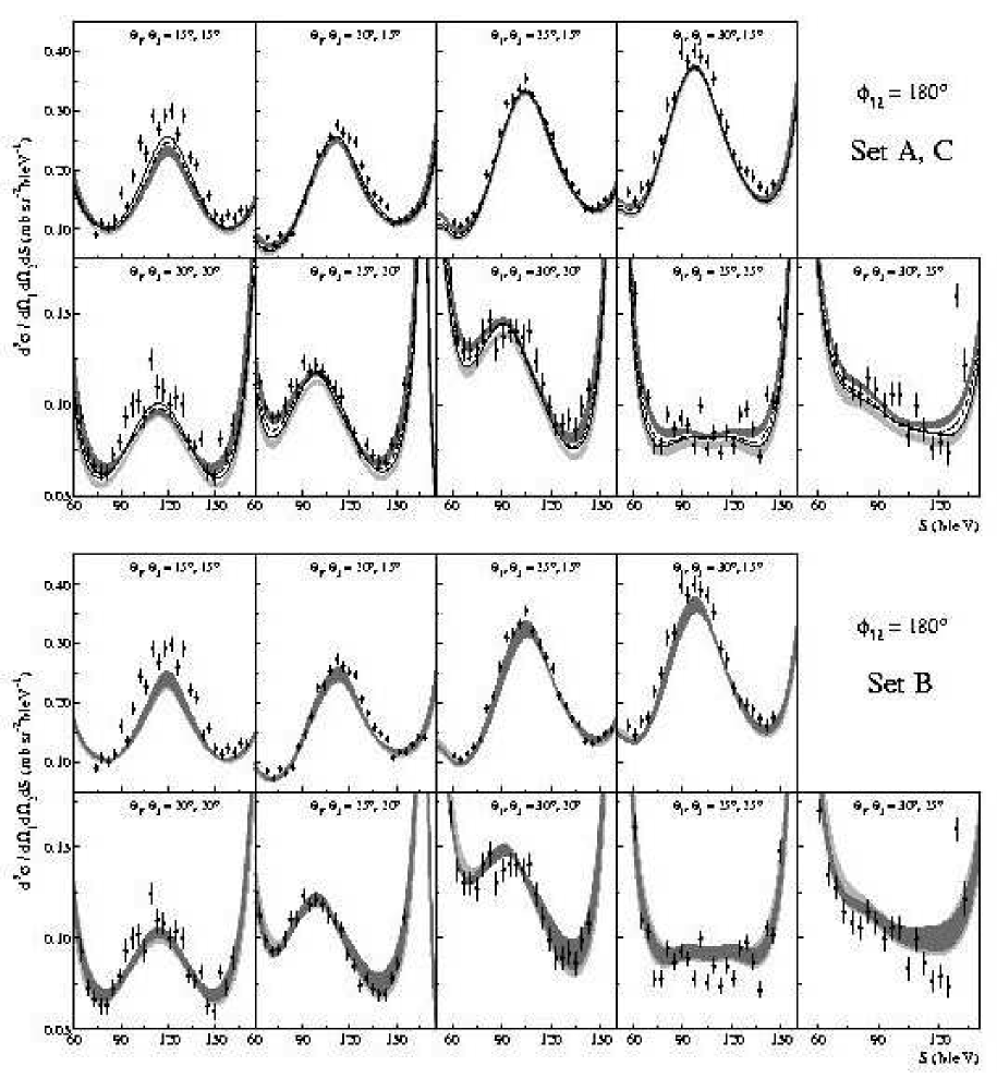
Figure 14: The same as in Fig. 7 but for kinematic configurations with the relative azimuthal angle of two protons $\phi_{12}$ = 180^∘.

IV.1 Individual kinematical configurations

A few geometries on the above defined grid were already presented in our previous report Kis03a . However, due to improvements in the analysis procedure discussed in Sec. II.2, the current results are slightly more precise. Therefore, and for the sake of presenting a complete picture of data comparison with various theoretical approaches, we display in Figs. 7-14 cross sections for all 72 kinematically complete configurations, each figure showing a collection of 9 geometries (different $\theta_{1}$, $\theta_{2}$ pairs) for the same value of the relative polar angle $\phi_{12}$. The data are compared with three sets of theoretical calculations, introduced in Sec. III. We refer to them by letters, corresponding to the numbering of the respective subsection: the realistic potential approach with model 3NF’s (Sec. III.1) is called “set A”, the ChPT predictions (Sec. III.2) are denoted by “set B” and the results for the coupled-channel potential with the explicit $\Delta$-isobar treatment (Sec. III.3) are called “set C”. Since the predictions of the three sets are often close to each other, in order to clearly demonstrate all the details, every figure is composed of two parts. In the upper part the data are confronted with the results of calculations of set A and set C. The light-shaded bands correspond to predictions obtained with only pairwise $NN$ potentials (AV18, CD Bonn, Nijm I and II), the dark-shaded bands show the results when they are combined with the 2$\pi$-exchange TM99 3NF. The dashed lines demonstrate the results of calculations with the AV18 potential combined with the Urbana IX 3NF. The solid lines show the predictions obtained with the use of the coupled-channel potential CD Bonn + $\Delta$. In the lower part the same data are shown with the predictions obtained at NNLO of the ChPT approach. The bands show the ranges of the results computed using the different cut-offs, listed in Eq. (10); the light-shaded bands display the results when the calculations were restricted to include only the $NN$ force contributions, the dark-shaded bands represent the predictions for the full dynamics, with the 3NF graphs taken into account. Following the arguments of our previous study Kis03a , we compare the experimental data averaged over finite phase-space intervals with the point-geometry theoretical predictions calculated at the central values of the ranges of the kinematical variables. It has been checked that for all the configurations considered here the averaging leads to a slight enhancement of the theoretical cross-section values, not exceeding 1.6%, equivalent to some extra normalization factor. Since the global conclusions are drawn mainly with eliminated influence of the data normalization (see further below), this simplification does not affect them.

Figs. 7-14 are the basis for the quantitative comparisons of our experimental results with the predictions obtained in different approaches, as well as between the theoretical calculations themselves.

There is a large number of configurations, concentrated mainly (but not exclusively) in the central region of the investigated azimuthal angle $\phi_{12}$ range (Figs. 10-11, top panels in Figs. 9,12-14), where predictions of all considered theoretical approaches are consistent with each other over the whole arclength range attainable in our experiment. This is particularly true for geometries characterized by relatively large values of the cross section. The bands representing ranges of cross section predicted by calculations with different realistic potentials (set A) converge practically to a common line, identical with the predictions of the coupled-channel potential (set C). Similarly, the bands reflecting the computation uncertainty of the ChPT approach (set B) are also very narrow. Generally, in those configurations the theoretical predictions follow very accurately the experimental distributions. This confirms the high quality of the predictions provided by modern formalisms and simultaneously reflects the precision and accuracy of the experiment. However, since the predictions with and without 3NF’s are identical, no details of the 3$N$ system dynamics can be gained from those data.

There are, however, regions of the phase space, where the results of the calculations incorporating 3NF contributions differ substantially from the ones using the $NN$ dynamics only. The most pronounced 3NF manifestations can be observed in the range $\phi_{12}>120^{\circ}$, in the configurations characterized by relatively small cross sections (Figs. 12-14). The induced changes concern the shape and/or the absolute magnitudes of the cross-section distributions. High sensitivity of the predicted cross sections to the details of the interaction model applied in the calculations makes this region extremely useful for studying the 3$N$ system dynamics. Regarding the results of the realistic potentials approaches (sets A and C), one observes that the inclusion of 3NF’s usually increases the predicted cross-section values and that the largest effects are introduced by the TM99 3NF model, slightly smaller ones for the case of Urbana IX 3NF and significantly smaller ones by the explicit $\Delta$-isobar excitation. The comparison of the calculated cross sections with the data leads to the important conclusion that the predictions of the realistic potentials describe the data much better when the contributions of the 3NF are taken into account. The ChPT results do not reveal that clear signal of the 3NF effects. Inclusion of the 3$N$ interaction components, if affecting the predictions at all, results in a small change of the shape of the cross-section distribution along $S$ rather than in modification of its absolute magnitude. In these geometries the bands representing the uncertainties of the ChPT predictions without and with the 3NF contributions are relatively wide, they essentially overlap one another, and generally their agreement with the data is satisfactory. One can also observe that the calculated cross sections practically coincide with the results of the realistic potential approach containing the full dynamics, i.e. with the 3NF model included.

In geometries with small azimuthal angle, $\phi_{12}\leq 80^{\circ}$ (Figs. 7-9), one can also identify several cases where the contributions of the TM99 or Urbana IX 3NF’s modify the predictions of the realistic potentials’ approach at an appreciable level. However, there are few reasons to consider the situation in this region as qualitatively different from that at large $\phi_{12}$ values. The coupled-channel calculations with $\Delta$-isobar excitation included predict cross-section values consistent with those obtained for realistic $NN$ potentials without the 3NF contributions. The set C predictions even tend to follow the lowest range of the set A band (see e.g. configuration $\theta_{1}$ = 25^∘, $\theta_{2}$ = 25^∘, $\phi_{12}$ = 40^∘ in Fig. 7). Although the ChPT predictions without and with 3NF contributions still significantly overlap, ranges of both kind of predictions are relatively small. As for set C, the set B predictions also agree rather well with the realistic potentials’ results, which do not include 3$N$ interaction effects. The comparison of theoretical results with the data shows noticeable disagreements for several geometries. Generally, all approaches, even if their results without and with 3NF contributions are almost identical (see e.g. configuration $\theta_{1}$ = 30^∘, $\theta_{2}$ = 15^∘, $\phi_{12}$ = 40^∘ in Fig. 7), overestimate the data. In geometries for which the two kinds of predictions differ, this inconsistency is worse for calculations with the 3NF contributions (TM99 or Urbana IX) taken into account, since adding this piece of dynamics increases the predicted cross-section values.

The discrepancy mentioned above is the largest for the configuration $\theta_{1}$ = 15^∘, $\theta_{2}$ = 15^∘, $\phi_{12}$ = 40^∘ (first panel of Fig. 7). All theoretical approaches (although the effect is slightly less pronounced for the ChPT predictions) deviate from the data by as much as 20%, i.e. far beyond the experimental uncertainties. Regarding all configurations characterized by the smallest analyzed proton polar angles, $\theta_{1}=\theta_{2}$ = 15^∘, one finds that the disagreement between the predictions and the experimental cross section changes systematically, with a strong dependence on the relative azimuthal angle: for the small $\phi_{12}$ values the data are overestimated, while for the large $\phi_{12}$ they are strongly underestimated. Only for $\phi_{12}$ around 100^∘ does the agreement become satisfactory. To a much smaller extent this effect is visible also for geometries with $\theta_{1}=\theta_{2}$ = 20^∘ and perhaps $\theta_{1}$ = 20^∘, $\theta_{2}$ = 15^∘. It should be noted that for all configurations characterized by a certain $\theta_{1}$, $\theta_{2}$ pair the same part of the detector is used to extract the data for any $\phi_{12}$ angle and, moreover, the efficiency corrections are tiny in comparison to the observed discrepancies, so it is impossible to attribute the inconsistencies to any experimental deficiency.

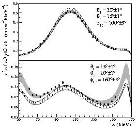
Figure 15: Comparison of experimental breakup cross sections in two kinematic configurations (indicated in the panels) with the predictions of ChPT performed at NNLO (dark-shaded bands) and at N³LO (hatched bands). Both calculations take into account only $NN$ force contributions.

The presented systematic study, covering a large fraction of the breakup phase space leads to a rather complicated picture. Generally, for most of the studied geometries the description of data provided by all theoretical approaches is quite satisfactory. There are specific regions, where the 3NF effects are pronounced and their importance is clearly confirmed by the measured cross sections. There are also final state geometries in which significant discrepancies between the experiment and the theoretical predictions are observed. The pattern of disagreement changes as a function of the kinematical variables. These findings strongly support the statement that only precise measurements in large regions of the phase space can provide enough information to judge on the quality of the models dealing with the description of the breakup observables. Resolving the discrepancies is at present not possible; they might be a signal of some missing ingredients in the assumed dynamics of the 3$N$ system.

Extending the investigation of the ChPT approach beyond the order discussed until now, we have compared our data with the predictions including only $NN$ contributions, obtained at the still higher, N³LO order – see Epe05a for details of the theory involved. Since the absence of 3NF contributions makes these calculations by virtue incomplete, we include the (incomplete) N³LO predictions only in global $\chi^{2}$ tests (see below). In Fig. 15 we present sample comparison of predictions obtained at NNLO (dark-shaded) and N³LO (hatched) for two geometries of the breakup reaction, both based on the $NN$ potential only. Comparing calculations based on incomplete dynamics can not be very conclusive, yet we can observe the differences between the obtained shapes, what may signal the importance of the higher order terms. It is also expected that the contributions of the 3NF at N³LO might be larger than at NNLO. The quantitative comparison, however, must be postponed until the full dynamics of the 3$N$ system is implemented at that order.

IV.2 Global comparisons

In order to perform a quantitative comparison of the whole bulk of our data with the theoretical predictions and to trace possible regularities in (dis-)agreement between data and theory, we continued the global tests initiated previously Kis03a , calculating values of $\chi^{2}$ per degree of freedom between the data and individual sets of theoretical predictions. We decided to concentrate on the option with a free normalization factor, putting more weight onto the shapes of the cross-section distributions as a function of $S$. In this way the conclusions are not biased by the absolute normalization uncertainties. In a later part of this Section we describe a complementary piece of investigation, presenting a comparison of data integrated over the arclength variable $S$ with the analogously treated theoretical predictions. There the experimental normalization is fully taken into account, while the dependence on $S$ (i.e. shape of the distribution) is to a large extent neglected. This approach is an example of studying the breakup phase space by inspecting its projections onto selected sub-spaces of lower dimensions.

Focusing our comparison on how the shapes of the cross-section distributions are reproduced by different theoretical approaches, we have calculated the values of $\chi^{2}$ per d.o.f. for all 72 configurations together (a total of nearly 1200 cross-section data points) with respect to all sets of theoretical predictions. The emphasis on the shapes of the distributions is motivated by the observation (cf. Sec. IV.1) that the action of 3NF contributions is usually equivalent to a small increase of the cross-section values in the whole range of $S$. Therefore, if the experimentally determined absolute normalization factor would be e.g. slightly too large, the data would be artificially shifted towards the predictions including full dynamics, leading to erroneous conclusions. This method also allows us to eliminate the small influence of averaging, inherently present in the data and omitted in the theoretical predictions (averaging does not affect the shapes of the cross-section distributions presented here). To eliminate the influence of the absolute experimental normalization, the data were renormalized in each configuration by a constant factor (limited to the range 0.9 to 1.1), to best fit the particular theoretical distribution. In this way the quality with which a given set of theoretical predictions reproduces all the data is quantified by a single number. In particular, for each combination of forces we can compare two $\chi^{2}$ values: $\chi^{2}_{2N}$ obtained for predictions based on pairwise $NN$ interaction only and $\chi^{2}_{2N+3N}$ for the calculations including 3NF contributions. It should be noted that in the $\chi^{2}$ analysis only statistical uncertainties were taken into account, therefore values exceeding 1 can be expected. Investigating influences of the 3NF effects we concentrate rather on the relative change from $\chi^{2}_{2N}$ to $\chi^{2}_{2N+3N}$ and not on the absolute $\chi^{2}$ value. The same argument holds when comparing predictions of different forces with respect to the quality with which they describe the experimental data.

Table 2: Agreement between the experimental cross sections and the theoretical predictions obtained in different approaches, quantified in terms of $\chi^{2}$ per degree of freedom. Major focus in comparing the data with theory is put on the shapes of the experimental distributions as explained in the text. The quality of the predictions based on only pairwise $NN$ interactions ($\chi^{2}_{2N}$) is compared with $\chi^{2}_{2N+3N}$ values obtained for calculations including genuine 3NF effects, typical for the particular approach. Details on the kinds of forces used in obtaining $\chi^{2}$ values at every row are given in the text.

$NN$ force	3NF model	$\chi^{2}_{2N}$	$\chi^{2}_{2N+3N}$
Set A
AV18	TM99	4.48	3.80
	Urbana IX		3.67
CD Bonn	TM99	4.04	3.80
Nijm I	TM99	4.38	4.38
Nijm II	TM99	4.53	4.05
Mean realistic	TM99	4.43	4.07
		(4.04-4.53)	(3.80-4.38)
Set B
ChPT at NNLO		3.67	3.96
		(3.36-6.59)	(3.35-6.64)
ChPT at N3LO		5.29	– –
Set C
Coupled-channel	$\Delta$-excitation	3.83	3.63

The results of the $\chi^{2}$ analysis for all considered theoretical approaches are shown in Table 2. First, the two kinds (without and with 3NF contributions included in the theory) of $\chi^{2}$ values are shown for 4 realistic $NN$ potentials and their combination with the TM99 3NF. The second row for the AV18 potential gives $\chi^{2}_{2N+3N}$ for this force combined with the Urbana IX 3NF. Excluding this last combination, we define a “mean realistic” prediction as a set of cross-section values given at each point ($\theta_{1}$,$\theta_{2}$,$\phi_{12}$,$S$) as a mean between the minimum and maximum cross section predicted by the 4 realistic forces (or their combination with TM99 3NF) at this kinematical point. The $\chi^{2}$ values with respect to this mean realistic prediction are also shown in Table 2, with the ranges, equal to the corresponding extreme $\chi^{2}$ values, repeated in the next row. These values are to be compared with the ones obtained for the ChPT calculations. In this case only the $\chi^{2}$ for the “mean” set is quoted. It is obtained analogously as in the realistic potentials case, as the central value between extremes predicted with 5 combinations of cut-offs. Also the ranges of $\chi^{2}$ values for predictions at NNLO are shown for comparison. In the case of N³LO calculations we quote only the central $\chi^{2}$, reminding the reader that the bands based on the $NN$ forces only tend to be wider at this computational order and therefore also the accuracy of the predictions would behave accordingly. The last row of Table 2 presents the results of $\chi^{2}$ analysis performed with respect to the coupled-channel potential. A small difference in $\chi^{2}_{2N}$ values for CD Bonn between set A and set C calculations is due to the different treatment of the charge dependence. The $\chi^{2}_{2N+3N}$ denotes here the value obtained for the calculations including all $\Delta$-isobar excitation effects.

Comparing the numbers presented in Table 2 one observes that combining any of the realistic potentials with a 3NF model improves the description of our data, decreasing the $\chi^{2}$ by about 10%. The effect varies for different $NN$ potentials of the set A calculations so that the ranges of $\chi^{2}_{2N}$ and $\chi^{2}_{2N+3N}$ values overlap. Nevertheless, a systematic shift of the predictions towards the data is visible for calculations including the full dynamics. Predictions obtained within the ChPT framework do not allow for such a conclusion. Although the quality of the data description for the set B calculations is very similar to that of the realistic potentials approach, the ranges of $\chi^{2}$ values obtained with and without 3NF contributions are very wide and overlap completely. The central-value predictions reveal even a slight worsening of the data description induced by including the 3NF effects. However, this observation is rather far fetched in view of large theoretical uncertainties and, moreover, taking the center of the relatively wide bands is not relevant for tracing details of the shapes of the distributions. The predictions of $NN$ force alone at N³LO show a much poorer agreement with the data than those of NNLO. Since the total 3NF contributions up to that order are expected to be larger than at NNLO, this effect might be easily compensated for by the complete dynamics included in the formalism. The set C calculations, with the coupled-channel potential and explicit $\Delta$-isobar degrees of freedom, lead in general to the smallest values of $\chi^{2}$. The effects of the $\Delta$ excitation are rather modest, but with their inclusion the predictions are moved by a few percent closer to the data. This conclusion is, however, biased by the absence of any estimate of the theoretical uncertainties.

As mentioned in Sec. IV.1, the largest disagreements between the data and the theoretical predictions are observed for configurations with the smallest polar angles, $\theta_{1}=\theta_{2}$ = 15^∘. In order to eliminate their possible dominant impact on the $\chi^{2}$ analysis, we have recalculated all the values of Table 2 excluding this piece of data (8 configuration out of 72). It has been found that the $\chi^{2}_{2N}$ and $\chi^{2}_{2N+3N}$ values obtained in that way were decreased only by about 5%, but the overall picture was preserved and thus all the above conclusions are valid also for that limited data sample. Below we present less global comparisons based on this subset of the data.

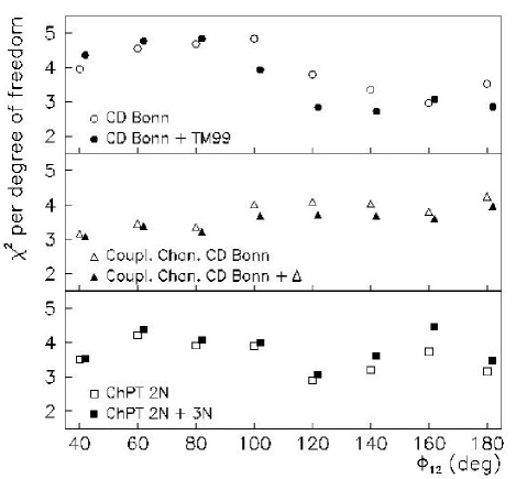
Figure 16: $\chi^{2}$ per degree of freedom calculated for groups of kinematical configurations with the same value of $\phi_{12}$. The results of data comparison with calculations of sets A, C and B are shown with dots, triangles and squares, respectively, in the separate panels. Empty and full symbols correspond to predictions based on $NN$ forces only and with the 3NF contributions included. For clarity the results for the full dynamics are artificially shifted along the $\phi_{12}$ axis by 2^∘.

To search for possible regularities in changes of the quality of the data description by the models, a less global treatment is obviously needed. Firstly, we studied the consistency between the data and theoretical predictions in various regions of the phase space, inspecting the dependence of $\chi^{2}$ on the relative azimuthal angle $\phi_{12}$ of the two protons. Values of $\chi^{2}$ have been calculated as in the global comparison case, but for the groups of configurations characterized by the same $\phi_{12}$ value, i.e. separately for each group presented in Figs. 7-14. The results are shown in Fig. 16 by three different symbols representing the three calculation sets and the $\chi^{2}_{2N}$ and $\chi^{2}_{2N+3N}$ shown by open and full symbols, respectively. To simplify the picture the realistic potentials are represented by the CD Bonn force (with and without TM99 3NF) and the ChPT approach results are shown for the mean set. One observes that for $\phi_{12}<90^{\circ}$ there is practically no effect of including the TM99 3NF into the calculations. For larger relative azimuthal angles the description of data is significantly improved by employing the full dynamics. The coupled-channel calculations predict much smaller effects due to $\Delta$ excitation, what is the result of a compensation mechanism, cf. Sec. III.3. Moreover, the quality of description depends only very weakly on $\phi_{12}$. The ChPT predictions do not show any large effects of 3NF contributions either. Only for the largest azimuthal angles, $\phi_{12}>120^{\circ}$, in contrast to the CD Bonn results, the full dynamics reproduces the data worse than calculations with $NN$ interaction terms only.

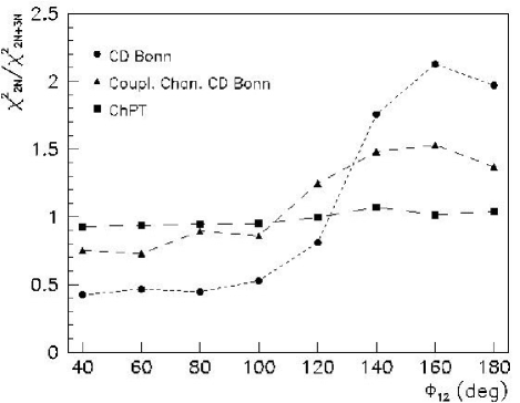
Figure 17: Ratios of $\chi^{2}$ values for calculations without and with 3NF contributions. The cross-section data with the experimental absolute normalization were used in computing the $\chi^{2}_{2N}$ and $\chi^{2}_{2N+3N}$ values for groups of kinematical configurations with the same $\phi_{12}$ angle. The results of data comparison with calculations of sets A, C and B are shown by dots, triangles and squares, respectively. The lines are only to guide the eye.

Pursuing the study of the $\chi^{2}$ dependence on the relative azimuthal angle, we have also checked the changes of quality of data description by calculations with and without 3NF contributions for the cross sections with absolute experimental normalization applied to the data. We present the results as the ratio of $\chi^{2}_{2N}$ to $\chi^{2}_{2N+3N}$ in order to magnify the influence of the $3NF$ effects. In Fig. 17 the ratios for the same theoretical sets as for the free normalization case are shown with the same symbols. One finds again that the consistency between the predictions of the CD Bonn potential and the data is improved by adding TM99 3NF in configurations with relatively large $\phi_{12}$ angles (ratio above 1). On the other hand, for $\phi_{12}<90^{\circ}$ including the 3NF into the calculations moves the results away from the data. Astonishingly, the magnitude of the relative change is almost the same in both directions, described by a factor of about 2. For the ChPT calculations no effect is present, the ratio stays close to 1 for all values of $\phi_{12}$. The behavior revealed by the set A predictions is qualitatively confirmed by the coupled-channel calculations, however the amplitude of the changes induced by including the $\Delta$-excitation contributions is smaller.

A great advantage of an experiment with the position sensitive detector covering a significant part of the phase space is the opportunity to study dependences of the observables (here the differential cross section) on all independent kinematic variables. However, inspecting the results in many-dimensional space is difficult and the comparisons with the theoretical predictions might miss the regularities. One possible solution to reduce the complexity of the problem and still be able to use all the data is to select a small number (e.g. 1 or 2) of variables and to integrate the observable over the others. Integration of the experimental data is usually quite straightforward – it is accomplished by summing up of events which fulfill the required conditions. But these experimental conditions (acceptances, thresholds, granularity, etc.) impose limitations, which make the procedure of integration for the theoretical predictions very complicated and the comparisons might be jeopardized by introducing uncontrollable systematic errors. A possible method to resolve the problem of comparing the integrated experimental and theoretical observables has been suggested in Kur04a . It allows to effectively integrate the calculated observables over all but one variables, with all experimental constraints taken into account. In the case of cross sections, however, such an approach leads to numerical values which are hard to interpret physically. Influences of the physical changes (due to reaction dynamics) of the observable are merged with the acceptance functions and the comparisons are meaningful only for “integrated physical values”. Therefore, in our first attempts to investigate regularities in the breakup phase space we rather employ a simpler method, deconvoluting the acceptances from the experimental results and comparing the integrated cross sections with the accordingly summed theoretical predictions. In this way we end up with “objective” cross-section values, with direct physical interpretation.

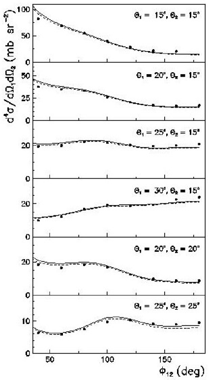
Figure 18: Differential, integrated over $S$, cross-section values, presented as functions of the relative azimuthal angle $\phi_{12}$, for several pairs of the proton polar angles $\theta_{1}$ and $\theta_{2}$ (indicated in the panels). The integration limits are defined by setting the proton energy threshold at 25 MeV. The data points are compared with the results of calculations with the CD Bonn potential (dashed lines) and with the CD Bonn + TM99 3NF combination of forces (solid lines).

The cross-section results for the individual configurations shown in Figs. 7-14 suggest a possible correlation between the polar and azimuthal angles with respect to the quality of the agreement between the data and predictions. Therefore, we studied the cross-section dependences on the proton emission angles with the experimental data integrated only over $S$. The energy threshold of the detection system introduces an inherent influence of the instrumental acceptance onto the result, but it is easy to reproduce without any detailed knowledge of other features of the apparatus. To guarantee an exact equivalence of the low-energy cut-off condition for the experimental and the predicted results, a threshold of 25 MeV (higher than the hardware level) was applied for both proton energies and only the range of $S$ limited by this requirement was included in the integration. The results for 6 pairs of the proton polar angles as functions of the relative azimuthal angle are shown in Fig. 18. The integrated experimental cross sections are compared to the correspondingly integrated theoretical predictions based on the CD Bonn potential only (dashed lines) and with the TM99 3NF included in the calculations (solid lines). It has been checked that the results for other realistic forces are almost indistinguishable from the ones presented in Fig. 18. The tendency, already visible in the cross-section plots for individual configurations, can be better traced here. For $\phi_{12}$ below $90^{\circ}$ the theoretical predictions overestimate the data and the discrepancy rises with decreasing $\phi_{12}$ values. In the central region of the analyzed $\phi_{12}$ range the agreement between the data and the theoretical curves is the best. With further increase of the $\phi_{12}$ angle the theoretical predictions start to underestimate the data. This discrepancy is, however, reduced (in various fractions) by including the 3NF into the calculations. On the contrary, for the small $\phi_{12}$ angles the effects of 3NF inclusion increase the discrepancies between the predictions and the data. It can be finally stated that in all cases studied in Fig. 18 the slope of the data, though qualitatively reproduced, is not exactly matched by the theoretical cross-section values and that overall rather small 3NF contributions do not change the global picture. Again, this has to be attributed to some still unresolved deficiencies of the models of the 3$N$ system dynamics.

Recapitulating all the results, from both the individual configurations of Figs. 7-14 and the global tests from this section, we can conclude, that the present day models of the 3$N$ system dynamics reproduce the majority of the data with satisfactory precision. In many cases in which the predicted effects due to 3NF’s are non-negligible, their inclusion tends to improve the agreement with the data. However, thanks to the applied experimental technique of covering a significant fraction of the breakup phase space with a highly symmetric detection system, it has been shown that there are also systematic regularities in the discrepancies between the measured cross sections and the predictions of all the theoretical approaches. Since the systematic factors of our measurement are common to all configurations, the established trends cannot be attributed to systematic experimental uncertainties and therefore hint at missing ingredients of the nuclear Hamiltonian models. It should also be stressed that additional complete and precise data sets, at other energies and in even larger phase space regions, are needed to study details of the interactions in the few-nucleon system.

V Summary and conclusions

A measurement of the deuteron-proton ¹H(d,pp)n breakup cross sections using a 130 MeV deuteron beam was performed for a large part of the available phase space. In this paper high precision, five-fold differential cross-section data for 72 kinematically complete configurations (total of nearly 1200 cross-section data points) at different angular combinations of the two outgoing protons are presented. We discuss first examples of a global analysis of the data, which is trying to establish possible regularities of the (dis-)agreement between the experimental data and different theoretical approaches.

We compare the measured cross sections to theoretical predictions treating the full dynamics of the 3$N$ system in three different ways: employing the realistic $NN$ potentials AV18, CD Bonn, Nijm I and Nijm II and including the 3NF effects by combining them with the TM99 3NF model (for AV18 also Urbana IX 3NF), obtaining the nuclear effective potential in the ChPT approach with the calculations performed at NNLO order with $NN$ and 3$N$ contributions (mentioning also the pure $NN$ results obtained at N³LO), and using the coupled-channel technique of explicit inclusion of a single $\Delta$-isobar degrees of freedom, resulting in a modified form of the realistic CD Bonn force and its combination with all single $\Delta$ excitation effects in the three-baryon system. The three approaches match equally well the properties of the $NN$ system. When only the 2$N$ dynamical sector is used, their predictions for the breakup cross sections are essentially equivalent.

The magnitude of the predicted 3NF effects depends on the approach. In the case of the coupled-channel potential the influences of the $\Delta$-isobar excitation are generally rather small. This is due to a competition of effects induced by two mechanisms, the two-baryon dispersion and the effective 3NF. ChPT predictions, considered in terms of ranges of the cross-section values computed with different cut-off parameters, reveal also rather weak contributions of the 3NF effects. They are usually smaller than the residual dependence on the cut-offs. Also the calculations at N³LO (presently available with $NN$ contributions only) are characterized by a broad range for the predicted cross-section values. The deviations of NNLO and N³LO predictions depend on the final state geometry. The largest sensitivity to the 3NF is found in the realistic potentials approach. But even for the realistic forces there are several final state geometries in which the 3NF effects are practically negligible. Generally, in such cases the cross-section data are in good agreement with the theoretical predictions. However, in many analyzed configurations the effects of including the 3NF are not negligible. Taking into account the 3NF contributions in the calculations leads to an increase of the cross-section values. This effect is slightly less pronounced for combining the Urbana IX 3NF with the AV18 $NN$ potential than for the TM99 force combined with any of the four considered $NN$ potentials.

A global analysis, focused on the shapes of the cross-section distributions as functions of the arclength variable $S$, shows that the agreement between the experimental data and the theoretical predictions improves when the 3NF contributions are taken into account. This conclusion is valid for all combinations of realistic $NN$ potentials with the model 3NF’s. While for the ChPT predictions no conclusions can be drawn due to essentially overlapping ranges of predictions without and with 3NF included, the coupled-channel calculations also reveal a slight improvement in the description of the data when the single $\Delta$-isobar excitation effects are incorporated.

There is, however, a number of configurations in which the cross-section data are not correctly reproduced by any calculation. The effect depends on the relative azimuthal angle $\phi_{12}$ of the two protons: for small values the data are overestimated by the predictions, the agreement becomes good in the central range of the analyzed $\phi_{12}$ and at the largest angles the discrepancy is reversed. Thanks to the highly symmetric form of our detection system, which allows to reduce and to carefully control and test for systematic uncertainties, we basically exclude the possibility of attributing this inconsistency to any experimental deficiency.

The regularities of disagreements have been studied in more detail using a global analysis, in which we have concentrated on both, the shapes of the distributions as well as on the absolute values of the cross sections. It has been established that for configurations with large values of the $\phi_{12}$ angle the agreement between the experimental data and the theoretical predictions is improved when the 3NF contributions are taken into account. On the contrary, for $\phi_{12}<100^{\circ}$ the 3NF effects move the predictions away from the data. This conclusion is valid for all combinations of realistic $NN$ potentials with the model 3NF’s. It also holds for the predictions obtained in the coupled-channel approach, but with reduced size of the effects induced by the $\Delta$-excitation. The ChPT calculations predict essentially no sensitivity to the 3NF influences along $\phi_{12}$.

We have confirmed that sizable influences of 3NF’s are visible in the breakup cross sections at the energy of our measurement. Comparison of the agreement between the experimental data and the predicted cross-section values is presented by first examples of analyzing a multi-dimensional breakup data set by inspecting its projections onto selected sub-spaces of lower dimensions. Since the advantages of the experimental method reduce strongly the impact of systematic errors, the established discrepancies might be considered as signal of some missing ingredients in the assumed dynamics of the 3$N$ system. Determining regularities in the disagreements might eventually help to identify shortcomings of the nuclear force models. However, it cannot be ruled out that the discrepancies result from Coulomb effects, which are ignored in all theoretical approaches presently used. In view of the recent advances in including long range forces into the Faddeev formalism this persisting question might soon be quantitatively addressed.

Our present study clearly shows the importance of complete, precise experiments, determining various observables of the breakup reaction. Implementing symmetric detection systems covering large fractions of the phase space allows to attain rich data sets, for which systematic uncertainties are strongly suppressed and well controlled. Results of such experiments are the basis for systematic comparisons with different theoretical approaches. They provide stringent criteria for verification of the models of the nuclear Hamiltonian, assumed in formulating the three-nucleon scattering problem. Further improvements of the theoretical models, which are also a basis for exact calculations in many-body systems, require still more experimental input. We are going to supplement the cross-section results with polarization observables, with which we will be able to provide more detailed information, and hopefully pin down the discrepancies found here. More data sets are needed, acquired at energies lower and higher than in our study, with proton and deuteron beams, as well as covering still larger fractions of the phase space.