Elastic scattering of low energy pions by nuclei and the in-medium isovector $\pi N$ amplitude

Measurements of elastic scattering of 21.5 MeV $\pi^{\pm}$ by Si, Ca, Ni and Zr were made using a single arm magnetic spectrometer. Absolute calibration was made by parallel measurements of Coulomb scattering of muons. Parameters of a pion-nucleus optical potential were obtained from fits to all eight angular distributions put together. The ‘anomalous’ $s$-wave repulsion known from pionic atoms is clearly observed and could be removed by introducing a chiral-motivated density dependence of the isovector scattering amplitude, which also greatly improved the fits to the data. The empirical energy dependence of the isoscalar amplitude also improves the fits to the data but, contrary to what is found with pionic atoms, on its own is incapable of removing the anomaly.

PACS numbers: 13.75.Gx; 21.30.Fe; 25.80.Dj

Corresponding author: E. Friedman, Tel: +972 2 658 4667, FAX: +972 2 658 6347,
E mail: elifried@vms.huji.ac.il

I Introduction

Interest in the pion-nucleus interaction at low energies has been focused recently on the $s$-wave part of the pion-nucleus optical potential. The so-called ‘anomalous’ repulsion of the $s$-wave pionic atom potential is the empirical finding, from fits of optical potential parameters to pionic atom data, that the strength of the repulsive $s$-wave potential inside nuclei is nearly double the value expected on the basis of the free $\pi N$ interaction. This has been known for almost two decades [1]. The enhancement results mostly from the in-medium isovector $s$-wave $\pi N$ amplitude which plays a dominant role due to the nearly vanishing of the corresponding isoscalar amplitude. Some extra repulsion comes also from the empirical dispersive component of the two-nucleon absorption term. The renewed interest in pionic atoms is based partly on the experimental observation of ‘deeply bound’ pionic atom states in the (d,³He) reaction [2, 3, 4, 5], the existence of which was predicted a decade earlier [6, 7, 8]. It is also based partly on attempts to explain the anomalous $s$-wave repulsion in terms of density dependence of the pion decay constant [9], or by constructing the $\pi N$ amplitude near threshold within a systematic chiral perturbation expansion [10, 11] and in particular imposing on it gauge invariance [12, 13].

Large scale fits to pionic atom data encompassing the whole of the periodic table showed [14, 15] that indeed the density-dependence of the pion decay constant [9] which causes the isosvector scattering amplitude to become density dependent, is capable of removing the anomaly. Similar conclusions were also presented [16, 4, 17, 5] on the basis of very restricted data sets, consisting mainly of the recently observed ‘deeply bound’ states of pionic atoms. Such analyses of small data bases inevitably rely on assumptions regarding some of the parameters of the potential, a method which also leads to unrealistic estimate of errors, as demonstrated [18] in a comparative study of uncertainties. It is interesting to note in this context that the deeply bound states have failed, so far, to provide information which is not available from the host of data regarding normal states. This is fully understood [19, 20] from arguments of overlap between the pionic wavefunction and the nucleus.

In an alternative approach large scale fits showed [21] that the anomaly can be removed by imposing the minimal substitution requirement [22] of $E\to E-V_{c}$, where $V_{c}$ is the Coulomb potential, on the properly constructed pion optical potential. In this case the removal of the anomaly is essentially thanks to the empirical energy dependence of the isoscalar scattering amplitude. This state of affairs makes it highly desirable to extend the experimental basis for studies of the pion-nucleus interaction at low energies and this is the topic of the present paper.

In the present work we extend the study of the $s$-wave term of the pion-nucleus potential by considering the elastic scattering of very low energy $\pi^{+}$ and $\pi^{-}$ on several nuclei. With the large number of scattering experiments performed in the first two decades of the ‘pion factories’, it is somewhat surprising to realize that at kinetic energies well below 50 MeV there seems to be only one set of high quality data available for both charge states of the pion obtained in the same experiment, namely, the data of Wright et al. [23] for 19.5 MeV pions on calcium. We have therefore performed precision measurements of elastic scattering of 21.5 MeV $\pi^{+}$ and $\pi^{-}$ on several nuclei in order to provide the necessary data. The purpose of this experiment is to study the behavior of the pion-nucleus potential across threshold into the scattering regime and to examine if the above-mentioned anomaly is observed also above threshold. Of particular importance is the question of whether the density dependence of the isovector amplitude or the empirical energy dependence of the isoscalar amplitude, which remove the anomaly in pionic atoms, are required by the scattering data. In the scattering scenario, unlike in the atomic case, one can study both charge states of the pion, thus increasing sensitivities to isovector effects and to the energy dependence of the isoscalar amplitude due to the Coulomb interaction. The present paper reports on precision measurements of elastic scattering of 21.5 MeV $\pi^{+}$ and $\pi^{-}$ by several nuclei and on the analysis of the data within an optical potential approach. A first account of this work has already been published [24].

Section II describes the experimental set-up and section III describes the data reduction and summarizes the experimental results. Section IV presents the analysis in terms of several versions of the pion-nucleus optical model. Section V is a summary.

II Experiment

A Experimental set-up

The aim of the experiment was to measure the differential cross sections for elastic $\pi^{+}$ and $\pi^{-}$ scattering off Si, Ca, Ni and Zr with sufficient energy resolution to separate the first excited states of the target nuclei and with high absolute accuracy. This was achieved with a single-arm experiment using a magnetic spectrometer which allowed scattering angles up to $120^{\circ}$ in the lab system.

The experiment was performed at the low-energy pion channel $\pi$E3 [25] of the Paul-Scherrer-Institute (PSI) at Villigen, Switzerland in its chromatic mode. The channel was designed to match the optical characteristics of the low-energy pion spectrometer LEPS that we used (see below). It is an S-type channel with a vertical bending plane resulting in an experimental area 6 m above floor level. It has a momentum acceptance of 3.4% FWHM , a momentum resolution of $<0.3\%$ and a length of 13 m. It focussed the pions on a beam spot of about 5 by 10 cm² on the target with a vertical dispersion of $-$5 cm/%. The target was mounted in air about 1 m downstream of the last quadrupole magnet of the channel and separated by thin Mylar windows from the vacua of the channel and of the spectrometer.

The dispersed beam spot demanded large area targets. We used self-supporting targets of Si, Ca, Ni and Zr of natural isotopic composition which were hanging on thin threads over the pivot point of the spectrometer. The target heights and widths ranged from 10 by 15 cm² for Si to 27 by 32 cm² for Zr and their areal densities amounted to 213, 325, 178 and 160 mg/cm² for Si, Ca, Ni and Zr, respectively. While Ni and Zr were simply chemically pure metallic plates the Si target was glued together from two layers of 5 by 5 cm² wafers. The Ca target consisted of 12 pieces of $\approx$ 4.4 by 4.8 by 0.2 cm³, cut from a block of Ca and also glued together with tiny amounts of glue. To minimize the energy loss and straggling of the pions in the targets their angle settings $\theta_{tgt}$ were always chosen such that the normal formed an angle of $\theta_{tgt}=\theta_{lab}/2$ with the beam direction where $\theta_{lab}$ is the spectrometer angle in the laboratory system.

The low-energy pion spectrometer LEPS [26, 27] consists of two dipole magnets in a split-pole configuration and a symmetric triplet of quadrupole magnets placed in front of the dipoles. In the intermediate focus a multiwire proportional chamber consisting of three vertical and three horizontal readout planes allows the measurement of position and angles of the trajectory. The focal plane is tilted by 43^∘ with respect to the central trajectory. This permits the use of a vertical drift chamber to determine the coordinate along the dispersive direction and the corresponding angle in the focal plane. The drift chamber is followed by two scintillation counters, each 10 mm thick, used for trigger purposes and by a range telescope consisting of six scintillation detectors of 15 mm thickness each, which is used for particle identification. More details are given in [27]. However, in addition to the set-up used previously we employed a thin (2 mm) plastic scintillator detector in front of the quadrupole triplet that supplied a precise timing signal which moreover is free of ambiguities, in contrast to the cyclotron RF-signal used in [27]. The resulting loss in energy resolution was insignificant relative to that produced by straggling in the targets, and the precise time-of-flight (TOF) measurement through the spectrometer improved the particle identification (see below).

The absolute normalisation of the cross sections for pion scattering is based on the so-called lepton normalisation developed for use with the LEPS-spectrometer [28]. In essence, the cross sections are obtained by measuring the yields of pions relative to elastic scattering of muons where the corresponding cross sections may be reliably calculated from the known charge distributions of the target nuclei. This way, quantities such as target thicknesses and effective solid angles play no role. The method employs a monitoring system [28] consisting of a muon telescope ring upstream of the target and a hodoscope placed 40 cm downstream of the target. The hodoscope consists of two planes of scintillator strips, 2 mm thick, in x- and y-direction, respectively, which allow TOF and intensity measurements over an area of 24 by 12 cm² with a pixel size of 1.5 by 1.5 cm². A 2 mm sheet of aluminum in front shielded the hodoscope against low-energy protons from the channel. The muon ring has been devised as a secondary low-rate beam monitor measuring the decay muons from pion decay in flight. It consisted of four scintillator telescopes mounted in a ring (up, down, right, left) around the incident beam direction with a directional sensitivity centered about 17^∘, well within the muon decay cone. Each of these passing telescopes consists of a pair of scintillators 70 by 15 by 3 mm³ coupled to miniature phototubes.

Finally, typical pion beam intensities were 0.5$\times 10^{6}$ sec^-1 for $\pi^{+}$ and 0.1$\times 10^{6}$ sec^-1 for $\pi^{-}$. The data acquisition system essentially remains as described in[27].

B Experimental procedure

The $\pi$E3 channel was set to a momentum of 82.4$\pm$0.3 MeV/c based on the momentum calibration of [27]. The magnetic fields of the LEPS-spectrometer were set to a nominal value of 69.4 MeV/c and the accepted momenta in its focal plane were in the range $-$15$\%\leq{\Delta p/p}\leq+20$%, where $\Delta p$ denotes the deviation from the central momentum. The energy resolution was about 0.4 MeV ($1\sigma$), enough to separate off the first excited states of all target isotopes with the exception of ⁴³Ca and ⁶¹Ni which, however, have an isotopic abundance of only 0.14% and 1.14%, respectively. Figure 1 shows examples of focal plane spectra for $\pi^{-}$ scattered from the Zr target at 80^∘ and 110^∘. In the latter case inelastically scattered pions are also observed. For the other targets and for most angles there was hardly any inelastic scattering observed.

Unambiguous particle identification in the focal plane was made possible in a 2D representation of TOF through the spectrometer vs. the TOF relative to the cyclotron RF signal, see Fig. 2. The splitting of the RF-TOF for the pions at the bottom of the figure (and for electrons at the top) had no consequences for the measurements as both parts of the pion peak were always summed. In addition to the loci of scattered pions, muons and electrons the signals from muons resulting from pion decay in the spectrometer were clearly discernible. The 2D analysis is essential as about two thirds of the pions leaving the target decayed before reaching the focal plane, producing a sizeable muon background there.

For the lepton normalisation it is essential to know the relative acceptance of the spectrometer which varies along the focal plane by over a factor of two [28]. The relative acceptance was measured by performing a “momentum scan” where the normalized yield of elastic scattering was measured as a function of the momentum setting of LEPS, for a fixed scattering angle and beamline tune. The relative normalisation was made both with the muon telescope ring and the beam hodoscope described above. In order to use the muon normalisation technique it is necessary to know the ratio between muon and pion beam intensities at the scattering target. The ratio on the hodoscope is available for each pixel and it could be extrapolated back to the target position with the help of Monte Carlo calculations, taking into account that muons which originate from pion decays near the hodoscope are still being identified by TOF as pions. The calculated ratios varied by less than $\pm$0.7% when varying the initial conditions of the calculation or the target material or angle. As a result of these simulations the $\mu/\pi$ ratios measured on the hodoscope had to be divided by 1.040$\pm$0.015 in order to get the ratios of genuine muons to pions on the target.

Two types of measurements of elastic scattering of muons were made. In the first type (‘self’ measurements), muons were recorded simultaneously with the pions, which was possible because muons appeared in the focal plane with slightly higher momentum than pions due to the different energy losses of pions and muons in the target, in the scintillation counter in front of the quadrupole triplet and in the vacuum windows. The relative yields were then corrected for the acceptances at the two locations. In addition and immediately after some pion measurements, designated ‘muon runs’ were made where the magnetic fields of LEPS were scaled up by 4.7% which moved the muons in the focal plane to the previous location of the pions. In this method there was no need to take into account the position dependence of the acceptance. However, this method was not practical at the largest angles due to the small cross sections. As is reported below, both methods yielded the same average normalisation constants within 2%, whereas the estimated errors of the ‘self’ and of the ‘muon runs’ methods were 7% and 5%, respectively.

III Data reduction and experimental results

Data reduction can be described as a series of cuts performed to finally define the events which are used to derive the required cross sections. The first cut was made in the focal plane angle vs. the intermediate focus angle, which removed many of the muons that originate from pion decays within the spectrometer. After such a decay the simple geometrical correlation between the two angles is lost and consequently this cut removed many of the decay muons, which at such low energies originate from close to 70% of the pions entering the spectrometer. The second cut was made in the 2D TOF spectra, such as shown in Fig. 2. The boundaries of the peaks were defined manually for each target and for every angle. In this cut elastically scattered pions or muons were selected, the latter related to beam muons (in contrast to decay muons) which served for the normalisation, as described above. The third cut was made on the coordinates at the target, defining a fixed area on the target from which particles were collected by the spectrometer. These coordinates were calculated by reconstructing the trajectory for each particle using the chamber readings at the focal plane and at the intermediate focus. The calculated trajectories were also used to correct the TOF through the spectrometer for any given momentum in order to improve the time resolution. The precise path length for each particle was also needed in order to calculate the pion-decay correction, which is very significant at such low energies. The resulting focal-plane spectra were then used to extract the areas under the peaks due to the elastic scattering with the help of Gaussian fits, including Landau tails. The normalisation of the beam was provided both by the muon telescope ring and by the hodoscope. Stability of the former was monitored by comparing the ratios of counts for the four different sides to their sum. The hodoscope provided the muon to pion ratios and it also enabled us to normalize muon runs directly on the muons of the beam.

The overall consistency and reliability of the determination of differential cross sections was demonstrated by the elastic scattering of muons. In the ‘self’ method results were available for all angles where pions were measured and the muon cross sections were rescaled to the pion position in the focal plane. In the ‘muon runs’ method the muon peak was already at the normal location of the pion peak and no rescaling was needed. The statistics was better for these runs but not all angles were measured. The relative cross sections were normalized at each angle by comparing measurements to predictions for Coulomb scattering from the known charge distributions of the target nuclei [29] using the computer program HADES [30] which was modified to describe elastic muon scattering as well. The uncertainty in the beam momentum causes uncertainties of 1.2 to 2.0% in the calculated $\mu^{+}$ cross sections, depending on angle, and uncertainties of 1.3 to 2.7% in the calculated $\mu^{-}$ cross sections. The uncertainties due to errors in the parameters of the nuclear charge distributions are smaller than 0.5%. The statistical errors of the ‘self’ method were in the range of 2 to 8% for $\mu^{+}$ and 3.5 to 15% for most of the $\mu^{-}$ measurements. For the ‘muon runs’ method the corresponding errors were 2% for $\mu^{+}$ and 2 to 3% for $\mu^{-}$. The weighted average normalisation constants for the two methods differed by 2% when their estimated errors were 7% and 5%, respectively. Consequently a common normalisation constant was chosen as the weighted average of both methods, with an estimated uncertainty of 4%. For 30^∘ a separate constant was used due to different setting of the channel slits. Figure 3 shows as an example comparisons between calculations and measurements for the Coulomb scattering of muons by Ni. Open circles and diamonds are for the two types of muon measurements, ‘self’ and ‘muon runs’, respectively. The 30^∘ points are not included because they do not have the same normalization constant as discussed above.

The pion cross sections were derived using the above average muon normalisations. There were insignificant differences between results based on the muon telescope ring and results based on the hodoscope for relative normalisation of the beam. The experimental muon to pion ratios were the averages taken from the hodoscope and corrected for the genuine ratios on the target, as described above. The nominal errors included the statistical errors and the errors on the average muon normalisation, which include also errors due to the focal plane position dependence of the acceptance of the spectrometer. Typical combined errors were in the range of 4-5% and although a careful analysis did not reveal any systematic effects, we chose to add quadratically an estimated normalisation error of 5% as done before with this spectrometer [27], when the muon normalisation method was compared with more conventional methods. These additional errors are included in the final errors presented here. Note that in the previous $\chi^{2}$ fits [24] it was found that the derived parameters of the optical potential did not depend on the precise values of the additional normalisation errors.

The experimental results are summarized in Tables I to IV. Because the target angle relative to the beam was always half of the spectrometer angle, the mid-target energy varied with angle in a range of up to 0.25 MeV . The cross sections presented were slightly corrected for these variations with the help of an optical model (see below) to a common energy for each target, which corresponds to the middle of that range.

IV Analysis

The analysis was performed with the conventional pion-nucleus optical potential as is widely used for analysing pionic atom data [1]. The Klein-Gordon equation is written as follows:

$$\left[\nabla^{2}+k^{2}-2\varepsilon^{(A)}_{red}(V_{{\rm opt}}+V_{c})+V^{2}_{c}\right]\psi=0~{}~{}~{}~{}(\hbar=c=1)$$ (1)

where $k$ and $\varepsilon^{(A)}_{red}$ are the wave number and reduced energy respectively in the c.m. system, $(\varepsilon^{(A)}_{red})^{-1}=E_{p}^{-1}+E_{t}^{-1}$ in terms of the c.m. energies for the projectile and target particles, respectively. $V_{c}$ is the finite-size Coulomb interaction of the pion with the nucleus, including vacuum-polarization terms. The optical potential for low energy pions is the well-known potential given by Ericson and Ericson [31],

$$2\varepsilon^{(A)}_{red}V_{{\rm opt}}(r)=q(r)+\vec{\nabla}\cdot\alpha(r)\vec{\nabla}$$ (2)

with

$$q(r) = -4\pi(1+\frac{\varepsilon^{(A)}_{red}}{M})\{{\bar{b}_{0}}(r)[\rho_{n}(r)+\rho_{p}(r)]+b_{1}[\rho_{n}(r)-\rho_{p}(r)]\}$$ (4)

$$-4\pi(1+\frac{\varepsilon^{(A)}_{red}}{2M})4B_{0}\rho_{n}(r)\rho_{p}(r),$$

$$\alpha(r)=\frac{\alpha_{1}(r)}{1+\frac{1}{3}\xi\alpha_{1}(r)}+\alpha_{2}(r),$$ (5)

where

$$\alpha_{1}(r)=4\pi(1+\frac{\varepsilon^{(A)}_{red}}{M})^{-1}\{c_{0}[\rho_{n}(r)+\rho_{p}(r)]+c_{1}[\rho_{n}(r)-\rho_{p}(r)]\},$$ (6)

$$\alpha_{2}(r)=4\pi(1+\frac{\varepsilon^{(A)}_{red}}{2M})^{-1}4C_{0}\rho_{n}(r)\rho_{p}(r).$$ (7)

In these expressions $\rho_{n}$ and $\rho_{p}$ are the neutron and proton density distributions normalized to the number of neutrons $N$ and number of protons $Z$, respectively, $M$ is the mass of the nucleon, $q(r)$ is referred to as the $s$-wave potential term and $\alpha(r)$ is referred to as the $p$-wave potential term. The function ${\bar{b}_{0}}(r)$ in Eq. (4) is given in terms of the local Fermi momentum $k_{\rm F}(r)$ corresponding to the isoscalar nucleon density distribution:

$${\bar{b}_{0}}(r)=b_{0}-\frac{3}{2\pi}(b_{0}^{2}+2b_{1}^{2})k_{\rm F}(r),$$ (8)

where $b_{0}$ and $b_{1}$ are minus the pion-nucleon isoscalar and isovector effective scattering lengths, respectively. The quadratic terms in $b_{0}$ and $b_{1}$ represent double-scattering modifications of $b_{0}$. In particular, the $b_{1}^{2}$ term represents a sizable correction to the nearly vanishing linear $b_{0}$ term. The coefficients $c_{0}$ and $c_{1}$ in Eq. (6) are the pion-nucleon isoscalar and isovector $p$-wave scattering volumes, respectively. The parameters $B_{0}$ and $C_{0}$ in Eqs. (4) and (7) represent $s$-wave and $p$-wave absorption, respectively, on pairs of nucleons and as such they have imaginary parts. Dispersive real parts are found to play an important role in pionic atom potentials. The terms with $4\rho_{n}\rho_{p}$ were originally written as $(\rho_{n}+\rho_{p})^{2}$, but the results hardly depend on which form is used. The parameter $\xi$ in Eq. (5) is the usual Ericson-Ericson Lorentz-Lorenz (EELL) coefficient [31]. An additional relatively small term, known as the ‘angle-transformation’ term (see Eq.(24) of [1]), is also included.

For pionic atoms the scattering lengths ($b_{0}$ and $b_{1}$) and scattering volumes ($c_{0}$ and $c_{1}$) are real but for the scattering case they become complex. At 21 MeV the imaginary parts of these parameters for the free pion-nucleon interaction are small, and in the present analysis, in order not to increase further the number of parameters, we assume only $B_{0}$ and $C_{0}$ to be complex. Note that in the preliminary analysis of the present data [24] we used complex $c_{0}$ and $c_{1}$ because we observed the need to make the $p$-wave absorption charge-dependent. Here we adhere to the pionic atoms approach but allow also such charge-dependence. The proton density distribution $\rho_{p}$ was obtained from the known charge density of the target nucleus by unfolding the finite size of the proton. For the neutrons we used an ‘average’ shape [32] with rms radii differences of $r_{n}-r_{p}$=$-$0.04, $-$0.05, 0.01 and 0.12 fm for Si, Ca, Ni and Zr, respectively. Calculations were made using for the densities the natural isotopic mixture of the targets as it was found to be an excellent approximation to calculations done separately for the various isotopes and then averaged.

Fits to the data were made by the usual least-squares method, handling all 72 cross sections at the same time. With at least 8 parameters in the potential and with correlations between some parameters it was always possible to get excellent fits with $\chi^{2}$ per degree of freedom very close to 1.0. In such circumstances it is necessary to apply constraints and physical considerations in order to get meaningful results. The rest of this section is devoted to results obtained by adopting this approach. Note, however, that in global analyses of pionic atom data covering the whole of the periodic table, it is found (e.g. in Ref. [15]) that all the parameters are quite well-determined.

First it was noticed that the $p$-wave scattering volumes $c_{0}$ and $c_{1}$ always came out very close to their corresponding free pion-nucleon values of 0.21 and 0.165 $m_{\pi}^{-3}$, respectively. Consequently, $c_{0}$ and $c_{1}$ were kept fixed at these values in subsequent fits. The EELL coefficient $\xi$ was also kept constant at 1.0. Without any additional restrictions on parameter values, it was found that the best fit was achieved with a very repulsive real part for the $s$-wave potential. That was clearly seen with $b_{0}$ being a factor 2-3 too repulsive compared to the free $\pi$N amplitude and with the dispersive Re$B_{0}$ approximately equal to $-$4Im$B_{0}$. Both results represent ‘anomalously’ large repulsion, which is parallel to the ‘anomalous repulsion’ in pionic atoms.

Next we turn to the isovector $s$-wave parameter $b_{1}$ which has been the topic of interest in recent years, as outlined in the Introduction. With the conventional model for the potential (denoted hereafter by C) $b_{1}$ is assumed to be constant, and then we get (see table V) $b_{1}=-0.114\pm 0.006~{}m_{\pi}^{-1}$, compared to the free pion-nucleon value [33] of $-0.088\pm 0.001~{}m_{\pi}^{-1}$, clearly exhibiting an ‘anomalous’ repulsion. In the Weise model [9] the in-medium $b_{1}$ is related to possible partial restoration of chiral symmetry in dense matter, as follows. Since $b_{1}$ in free-space is well approximated in lowest chiral-expansion order by the Tomozawa-Weinberg expression [34]

$$b_{1}=-\frac{\mu_{\pi N}}{8\pi f^{2}_{\pi}}=-0.08~{}m^{-1}_{\pi}\,,$$ (9)

then it can be argued that $b_{1}$ will be modified in pionic atoms if the pion decay constant $f_{\pi}$ is modified in the medium. The square of this decay constant is given, in leading order, as a linear function of the nuclear density,

$$f_{\pi}^{*2}=f_{\pi}^{2}-\frac{\sigma}{m_{\pi}^{2}}\rho$$ (10)

with $\sigma$ the pion-nucleon sigma term. This leads to a density-dependent isovector amplitude such that $b_{1}$ becomes

$$b_{1}(\rho)=\frac{b_{1}(0)}{1-2.3\rho}$$ (11)

for $\sigma$=50 MeV [35] and with $\rho$ in units of fm^-3. This model which was shown [14, 15] to explain the anomaly in pionic atoms, is denoted here by W. An alternative approach which was also shown to explain the anomaly in pionic atoms [21] is to replace $E$ by $E-V_{c}$ by imposing the minimal substitution requirement [22], which is effective through the energy dependence of the isoscalar parameter $b_{0}$. This model is denoted here by E. Finally, applying both mechanisms we have the EW model.

Table V summarizes the parameters of the optical potentials obtained for the various models with the constraints of (i) $b_{0}$ in the range [33] of $-0.008$ to $-0.010~{}m_{\pi}^{-1}$ and (ii) Re$B_{0}$ close to $-$Im$B_{0}$ (see Ref.[1]). For the empirical parameter Im$C_{0}$ we introduced the option of energy dependence, implemented as

$${\rm Im}C_{0}~{}=~{}{\rm Im}C_{0}^{0}~{}+\alpha V_{c}$$ (12)

but the parameter $\alpha$ turned out to be consistent with zero except for the EW model. The last row in the table, marked as EW^∗, is for the potential EW with this energy dependence of Im$C_{0}$. The slope parameter in that case is $\alpha=-0.003\pm 0.001~{}m_{\pi}^{-6}$ MeV^-1, which implies good consistency between pionic atoms and the potential at 21 MeV. It is seen from Table V that the fit due to the conventional potential (C) is very significantly improved by introducing the density dependence of $b_{1}$, the energy dependence of $b_{0}$ or both. The derived values of $b_{1}$ agree with the free pion-nucleon value of $-0.088\pm 0.001~{}m_{\pi}^{-1}$ only when the density dependence is included in the model. Figures 4 and 5 show comparisons between experiment and calculation for the EW potential. It is self evident that the calculations reproduce all the features of the data.

The success of the W model is easy to understand since the density dependence introduced by Weise [9] provides enhanced $s$-wave repulsion in the nuclear medium. The observation that the agreement between calculation and experiment improves when the energy dependence of the parameter $b_{0}$ is included is also easy to understand. Out of the scattering lengths and scattering volumes for the free $\pi N$ interaction at low energies the isoscalar scattering length $b_{0}$ has the strongest energy dependence [33], and coupled with its very small values that energy dependence is significant. By adopting the minimal substitution requirement [22] of $E\to E-V_{c}$ and using the empirical slope of $b_{0}(E)$, the effects of the Coulomb attraction or repulsion are taken into account. In the scattering scenario it causes the effective values of $b_{0}$ to be different for the two charge states of the pion, and that is favoured by the data. The quadratic terms of the potential, namely, $B_{0}$ and $C_{0}$, remain empirical and are determined to a rather low accuracy. Only for the EW* model there is an indication that Im$C_{0}$ might be energy dependent.

V Summary

Precision measurements of elastic scattering of 21.5 MeV $\pi^{\pm}$ by targets of Si, Ca, Ni and Zr have been made in order to provide an experimental basis for determining parameters of the pion-nucleus optical potential. Emphasis was placed on the ‘anomalous’ $s$-wave repulsion, well known from global fits to pionic atom data. The experiment used a single arm magnetic spectrometer which enabled efficient particle identification and rejection of the large muon background, typical of such low energies. The absolute scale and the validity of the shapes of angular distributions measured for pions were established by parallel measurements of the Coulomb scattering of muons by the same target nuclei. The data were analyzed with optical potentials known from fits to pionic atom data. Very good fits to the elstic scattering data were obtained with extension to 21 MeV of several of the commonly accepted pionic atoms potentials. The ‘anomalous’ $s$-wave repulsion was clearly observed, and could be accounted for by introducing a chiral-motivated density dependence of the isovector scattering amplitude, as is the case with pionic atoms. This density dependence that enhances the isovector $s$-wave amplitude in the nuclear medium, also improves significantly the fit to the data. Introducing into the potential the empirical energy dependence of the $s$-wave isoscalar amplitude, motivated by the minimal substitution requirement of $E\to E-V_{c}$ and using the empirical slope of $b_{0}(E)$, greatly improves the fits to the data. However, this effect on its own is incapable of explaining the ‘anomaly’ at 21 MeV, unlike the situation with pionic atoms. In all cases the linear terms of the pion-nucleus potential connect smoothly to the corresponding quantities obtained from fits to pionic atom data. In contrast the empirical quadratic terms are quite different from the corresponding values for pionic atoms. However, when both the density dependence and the energy dependence mechanisms are included in the model, it is found that making the $p$-wave absorption term energy-dependent, via the Coulomb potential, further improves the fits to the data. In that case the $p$-wave absorption term also connects smoothly to the pionic atoms value.

This work was supported in part by the German ministry of education and research (BMBF) under contracts 06 TU 987I and 06 TU 201 and the Deutsche Forschungsgemeinschaft (DFG) through European Graduate School 683 and Heisenberg Program.

TABLE I.: Experimental results for 21.69 MeV $\pi^{\pm}$ scattering from Si.

c.m. angle (∘)	$\pi^{+}~{}~{}d\sigma/d\Omega$ (mb/sr)	$\pi^{-}~{}~{}d\sigma/d\Omega$ (mb/sr)
30.15	121.4 $\pm$ 9.6	149.7 $\pm$ 11.7
40.19	43.5 $\pm$ 3.2	38.5 $\pm$ 3.1
50.23	20.4 $\pm$ 1.7	10.6 $\pm$ 0.9
60.25	15.6 $\pm$ 1.2	7.1 $\pm$ 0.5
70.28	13.5 $\pm$ 1.1	6.1 $\pm$ 0.5
80.29	13.2 $\pm$ 1.0	7.3 $\pm$ 0.8
90.30	11.1 $\pm$ 1.0	10.9 $\pm$ 1.2
100.29	11.2 $\pm$ 1.0	14.7 $\pm$ 1.6
110.28	12.4 $\pm$ 1.3	17.0 $\pm$ 2.9

TABLE II.: Experimental results for 21.05 MeV $\pi^{\pm}$ scattering from Ca.

c.m. angle (∘)	$\pi^{+}~{}~{}d\sigma/d\Omega$ (mb/sr)	$\pi^{-}~{}~{}d\sigma/d\Omega$ (mb/sr)
30.11	243.9 $\pm$ 16.6	312.7 $\pm$ 21.1
40.13	79.6 $\pm$ 5.4	82.9 $\pm$ 5.7
50.16	41.4 $\pm$ 2.8	25.1 $\pm$ 1.7
60.18	28.1 $\pm$ 1.9	12.3 $\pm$ 0.8
70.19	20.8 $\pm$ 1.4	13.6 $\pm$ 0.9
80.20	18.0 $\pm$ 1.2	19.5 $\pm$ 1.3
90.21	16.6 $\pm$ 1.1	24.7 $\pm$ 1.7
100.20	15.5 $\pm$ 1.1	25.6 $\pm$ 1.7
110.20	14.9 $\pm$ 1.0	23.2 $\pm$ 1.6

TABLE III.: Experimental results for 21.45 MeV $\pi^{\pm}$ scattering from Ni.

c.m. angle (∘)	$\pi^{+}~{}~{}d\sigma/d\Omega$ (mb/sr)	$\pi^{-}~{}~{}d\sigma/d\Omega$ (mb/sr)
30.07	479.5 $\pm$ 31.2	502.6 $\pm$ 33.7
40.09	156.0 $\pm$ 10.4	137.1 $\pm$ 9.2
50.11	77.8 $\pm$ 5.2	44.2 $\pm$ 3.0
60.12	44.9 $\pm$ 3.0	30.5 $\pm$ 2.1
70.13	32.5 $\pm$ 2.2	35.4 $\pm$ 2.4
80.14	26.8 $\pm$ 1.8	43.0 $\pm$ 2.9
90.14	21.3 $\pm$ 1.4	41.5 $\pm$ 2.8
100.14	17.8 $\pm$ 1.2	32.6 $\pm$ 2.2
110.13	16.0 $\pm$ 1.1	22.4 $\pm$ 1.5

TABLE IV.: Experimental results for 21.70 MeV $\pi^{\pm}$ scattering from Zr.

c.m. angle (∘)	$\pi^{+}~{}~{}d\sigma/d\Omega$ (mb/sr)	$\pi^{-}~{}~{}d\sigma/d\Omega$ (mb/sr)
30.05	943.6 $\pm$ 62.1	875.4 $\pm$ 58.8
40.06	287.9 $\pm$ 19.5	222.5 $\pm$ 15.1
50.07	129.3 $\pm$ 8.7	95.2 $\pm$ 6.5
60.08	73.0 $\pm$ 4.9	96.7 $\pm$ 6.5
70.09	50.3 $\pm$ 3.4	96.5 $\pm$ 6.5
80.09	33.9 $\pm$ 2.3	75.9 $\pm$ 5.1
90.09	25.3 $\pm$ 1.7	39.7 $\pm$ 2.7
100.09	21.5 $\pm$ 1.5	22.4 $\pm$ 1.5
110.09	18.1 $\pm$ 1.2	8.3 $\pm$ 0.6

TABLE V.: Optical potential parameters from fits to elastic scattering of 21.5 MeV $\pi^{\pm}$ by Si, Ca, Ni and Zr. Values of $b_{0}$ were kept in the range of $-$0.008 to $-$0.010 $m_{\pi}^{-1}$ and values of $c_{0}$ and $c_{1}$ were held fixed at the free pion-nucleon values of 0.21 and 0.165 $m_{\pi}^{-3}$, respectively. Values of Re$B_{0}$ were held fixed. For the EW^∗ model Coulomb dependence of Im$C_{0}$ was included, see Eq. (12). The various models are defined in the text

model	$b_{1}(m_{\pi}^{-1}$)	Re$B_{0}(m_{\pi}^{-4}$)	Im$B_{0}(m_{\pi}^{-4}$)	Re$C_{0}(m_{\pi}^{-6}$)	Im$C_{0}(m_{\pi}^{-6}$)	$\chi^{2}$ for 72 points
C	$-$0.114$\pm$0.006	$-$0.040	0.035$\pm$0.007	$-$0.030$\pm$0.020	0.075$\pm$0.035	134
W	$-$0.081$\pm$0.005	$-$0.040	0.040$\pm$0.007	$-$0.045$\pm$0.015	0.062$\pm$0.030	88
E	$-$0.119$\pm$0.006	$-$0.025	0.025$\pm$0.005	$-$0.022$\pm$0.012	0.085$\pm$0.027	80
EW	$-$0.083$\pm$0.005	$-$0.025	0.023$\pm$0.005	$-$0.023$\pm$0.012	0.130$\pm$0.025	88
EW∗	$-$0.083$\pm$0.005	$-$0.025	0.018$\pm$0.004	$-$0.010$\pm$0.009	0.140$\pm$0.020	72

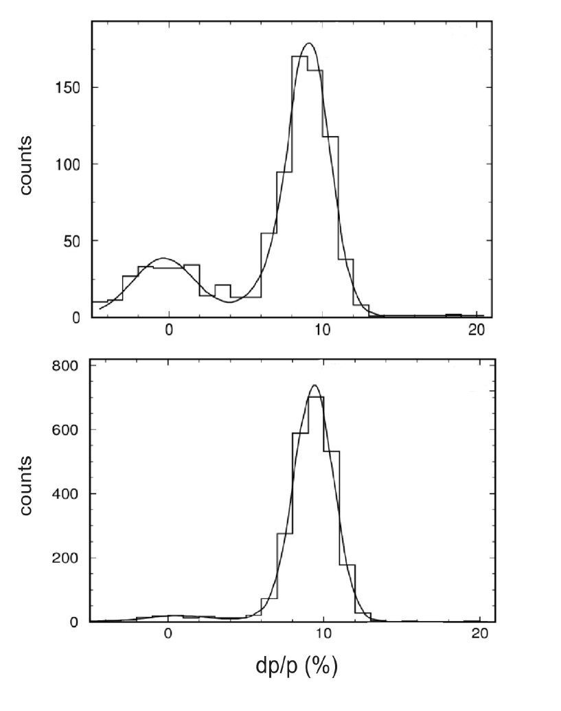
FIG. 1.: Examples of focal-plane spectra for $\pi^{-}$ scattered by Zr at 110^∘ (upper part) and at 80^∘ (lower part). A peak due to inelastic scattering is clearly seen at 110^∘.

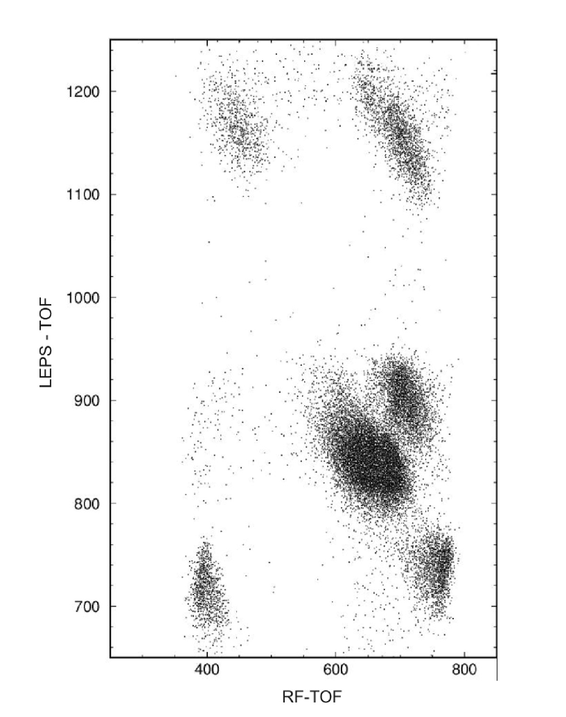
FIG. 2.: TOF within the LEPS spectrometer vs. TOF relative to the cyclotron RF, in arbitrary units, showing clear separation of the various types of particles. Pions are at the bottom and electrons are at the top of the figure. The central groups are due to beam muons (right) and decay muons.

FIG. 3.: Coulomb scattering of muons by Ni. Open circles: ‘self’ method. open diamonds: ‘muon runs’ method. Continuous curves are calculated Coulomb scattering for the finite size charge distribution. Common normalization constants have been used, separately for all the $\mu^{+}$ points and all the $\mu^{-}$ points, see text.

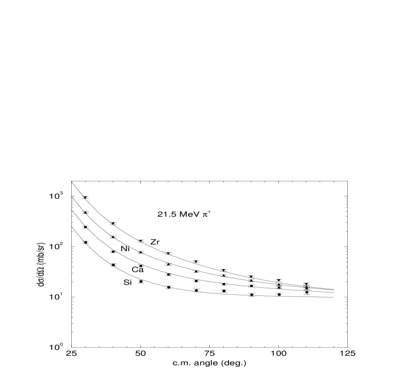
FIG. 4.: Experimental results for $\pi^{+}$ compared to predictions for potential EW of Table V. Potential parameters were obtained from fits to the combined data for $\pi^{+}$ and $\pi^{-}$.

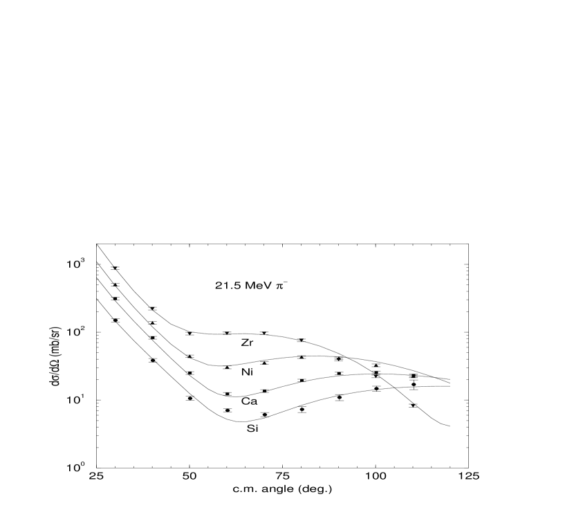
FIG. 5.: Experimental results for $\pi^{-}$ compared to predictions for potential EW of Table V. Potential parameters were obtained from fits to the combined data for $\pi^{+}$ and $\pi^{-}$.

REFERENCES

- [1] For early references see C.J. Batty, E. Friedman and A. Gal, Phys. Rep. 287, 385 (1997).
- [2] T. Yamazaki, R.S. Hayano, K. Itahashi, K. Oyama, A. Gillitzer, H. Gilg, M. Knülle, M. Münch, P. Kienle, W. Schott, H. Geissel, N. Iwasa and G. Münzenberg, Z. Phys. A 355, 219 (1996).
- [3] H. Gilg, A. Gillitzer, M. Knülle, M. Münch, W. Schott, P. Kienle, K. Itahashi, K. Oyama, R.S. Hayano, H. Geissel, N. Iwasa, G. Münzenberg and T. Yamazaki, Phys. Rev. C 62, 025201 (2000).
- [4] H. Geissel, H. Gilg, A. Gillitzer, R.S. Hayano, S. Hirenzaki, K. Itahashi, M. Iwasaki, P. Kienle, M. Münch, G. Münzenberg, W. Schott, K. Suzuki, D. Tomono, H. Weick, T. Yamazaki and T. Yoneyama, Phys. Rev. Lett. 88, 122301 (2002).
- [5] K. Suzuki, M. Fujita, H. Geissel, H. Gilg, A. Gillitzer, R.S. Hayano, S. Hirenzaki, K. Itahashi, M. Iwasaki, P. Kienle, M. Matos, G. Münzenberg, T. Ohtsubo, M. Sato, M. Shindo, T. Suzuki, H. Weick, M. Winkler, T. Yamazaki and T. Yoneyama, Phys Rev. Lett. 92, 072302 (2004).
- [6] E. Friedman and G. Soff, J. Phys. G: Nucl. Phys. 11, L37 (1985).
- [7] H. Toki and T. Yamazaki, Phys. Lett. B 213, 129 (1988).
- [8] H. Toki, S. Hirenzaki, T. Yamazaki and R.S. Hayano, Nucl. Phys. A 501, 653 (1989).
- [9] W. Weise, Nucl. Phys. A 690, 98c (2001).
- [10] N. Kaiser and W. Weise, Phys. Lett. B 512, 283 (2001).
- [11] U.G. Meissner, J.A. Oller and A. Wirzba, Ann. Phys. (NY) 297, 27 (2002).
- [12] E.E. Kolomeitsev, N. Kaiser and W. Weise, Phys. Rev. Lett. 90, 092501 (2003).
- [13] E.E. Kolomeitsev, N. Kaiser and W. Weise, Nucl. Phys. A 721, 835c (2003).
- [14] E. Friedman, Phys. Lett. B 524, 87 (2002).
- [15] E. Friedman, Nucl. Phys. A 710, 117 (2002).
- [16] P. Kienle and T. Yamazaki, Phys. Lett. B 514, 1 (2001).
- [17] H. Geissel et al., H. Gilg, A. Gillitzer, R.S. Hayano, S. Hirenzaki, K. Itahashi, M. Iwasaki, P. Kienle, M. Münch, G, Münzenberg, W. Schott, K. Suzuki, D. Tomono, H. Weick, T. Yamazaki and T. Yoneyama, Phys. Lett. B 549, 64 (2002).
- [18] E. Friedman and A. Gal, Nucl. Phys. A 724, 143 (2003).
- [19] E. Friedman and A. Gal, Phys. Lett. B 432, 235 (1998).
- [20] E. Friedman and A. Gal, Nucl. Phys. A 721, 842c (2003).
- [21] E. Friedman and A. Gal, Phys. Lett. B 578, 85 (2004).
- [22] T.E.O. Ericson and L. Tauscher, Phys. Lett. B 112, 425 (1982).
- [23] D.H. Wright,M. Blecher, B. G. Ritchie, D. Rothenberger, R. L. Burman, Z. Weinfeld, J. A. Escalante, C. S. Mishra, and C. S. Whisnant, Phys. Rev. C 37, 1155 (1988).
- [24] E. Friedman, M. Bauer, J. Breitschopf, H. Clement, H. Denz, E. Doroshkevich, A. Erhardt, G.J. Hofman, R. Meier, G.J.Wagner, G. Yaari, Phys. Rev. Lett. 93, 122302 (2004).
- [25] F. Foroughi (1997) http://people.web.psi.ch/foroughi/.
- [26] H.Matthäy, K.Göring, J.Jaki, W.Kluge, M.Metzler and U. Wiedner, Proc. Int. Symposium on Dynamics of Collective Phenomena in Nuclear and Subnuclear Long Range Interactions in Nuclei, Bad Honnef, Germany, May 4-7 1987, ed. Peter David, World Scientific, Singapore, New Jersey, Hong Kong.
- [27] Ch. Joram, M. Metzler, J. Jaki, W. Kluge, H. Matthäy, R. Wieser, B.M. Barnett, H. Clement, S. Krell and G.J. Wagner, Phys. Rev. C 51, 2144 (1995).
- [28] B.M. Barnett, S. Krell, H. Clement, G.J. Wagner, J. Jaki, Ch. Joram, W. Kluge, H. Matthäy and M. Metzler, Nucl. Inst. Methods A 297, 444 (1990).
- [29] G. Fricke, C. Bernhardt, K. Heilig, L.A. Schaller, L. Schellenberg, E.B. Shera, C.W. De Jager, At. Data Nucl. Data Tables 60, 177 (1995).
- [30] H.G.Andresen, H. Peter, M. Müller, H.J.Ohlbach and P.Weber, Program HADES, Universität Mainz (1986), unpublished.
- [31] M. Ericson, T.E.O. Ericson, Ann. Phys. (NY) 36, 323 (1966).
- [32] E. Friedman, A. Gal, Nucl. Inst. Methods B 214, 160 (2004).
- [33] http://gwdac.phys.gwu.edu/
- [34] Y. Tomozawa, Nuovo Cimento A 46, 707 (1966); S. Weinberg, Phys. Rev. Lett. 17, 616 (1966).
- [35] J.Gasser, H. Leutwyler and M.E. Sainio, Phys. Lett. B 253, 252 (1991).