Nuclear fusion in muonic deuterium-helium complex

Abstract

Experimental study of the nuclear fusion reaction in charge-asymmetrical $d\mu{}^{3}\mathrm{He}$ complex ($d\mu{}^{3}\mathrm{He}\rightarrow\alpha$ (3.5 MeV) + $p$ (14.64 MeV)) is presented. The 14.64 MeV protons were detected by three pairs of Si($dE-E$) telescopes placed around the cryogenic target filled with the $\mathrm{D}_{2}+{}^{3}\mathrm{He}$ gas at 34 K. The 6.85 keV $\gamma$ rays emitted during the de-excitation of the $d\mu{}^{3}\mathrm{He}$ complex were detected by a germanium detector. The measurements were performed at two $\mathrm{D}_{2}+^{3}\mathrm{He}$ target densities, $\varphi=0.0585$ and $\varphi=0.169$ (relative to liquid hydrogen density) with an atomic concentration of ${}^{3}\mathrm{He}$ $c_{{}^{3}\mathrm{He}}=0.0469$. The values of the effective rate of nuclear fusion in $d\mu{}^{3}\mathrm{He}$ was obtained for the first time: $\tilde{\lambda}_{f}=(4.5^{+2.6}_{-2.0})\times 10^{5}\,\mbox{s}^{-1}(\varphi=0.0585)$; $\tilde{\lambda}_{f}=(6.9^{+3.6}_{-3.0})\times 10^{5}\,\mbox{s}^{-1}(\varphi=0.168)$. The $J=0$ nuclear fusion rate in $d\mu{}^{3}\mathrm{He}$ was derived: $\lambda^{J=0}_{f}=(9.7^{+5.7}_{-2.6})\times 10^{5}\,\mbox{s}^{-1}\ (\varphi=0.0585)$; $\lambda^{J=0}_{f}=(12.4^{+6.5}_{-5.4})\times 10^{5}\,\mbox{s}^{-1}\ (\varphi=0.168)$.

I Introduction

The formation of muonic molecules of hydrogen isotopes and their nuclear reactions have been the subject of many experimental and theoretical studies Marshall et al. (2001); Petitjean (2001, 1992); Cohen (1990/91); Ponomarev (1990, 2001); Nagamine (2001); Bogdanova and Markushin (1990). As to the studies of formation of charge-asymmetrical muonic molecules like $h\mu Z$ ($h=p,d,t$, $Z$ are nuclei with a charge $Z>1$) and their respective nuclear fusion, the situation slightly different. What gave an impetus to study such systems was the theoretical prediction and experimental observation of the molecular mechanism for charge exchange (MMCE) of $p\mu$ atoms on He nuclei Aristov et al. (1981); Bystritsky et al. (1983). Essentially, the mechanism is reduced to the following. Colliding with a He atom in a $H$–He mixture ($H=\mathrm{H}_{2},\mathrm{D}_{2},\mathrm{T}_{2}$ and $\mathrm{He}={}^{3}\mathrm{He},{}^{4}\mathrm{He}$), the muonic hydrogen atom forms a muonic complex $h\mu\mathrm{He}$ in the excited $2p\sigma$ state. In the case of a deuterium–helium mixture, the complex may then decays from this state (see Fig. 1) via one of three channels

$$d\mu+{\mathrm{He}}\stackrel{{\scriptstyle\lambda_{d\mathrm{He}}}}{{\longrightarrow}} \ [(d\mu{\mathrm{He}})^{*}e^{-}]^{+} +\ e^{-}\mbox{ \hskip 36.135pt\ }$$

$$\hskip 17.07182pt\downarrow$$

$$\ \ \ \ \stackrel{{\scriptstyle\lambda_{\gamma}}}{{\longrightarrow}} [(d\mu{\mathrm{He}})^{+}e^{-}]+\gamma$$ (1a)

$$\ \ \ \ \stackrel{{\scriptstyle\lambda_{p}}}{{\longrightarrow}} [(\mu{\mathrm{He}})^{+}_{1s}e^{-}]+d$$ (1b)

$$\ \ \ \ \stackrel{{\scriptstyle\lambda_{e}}}{{\longrightarrow}} (\mu{\mathrm{He}})^{+}_{1s}+d+e^{-}\,.$$ (1c)

If $\mathrm{He}={}^{3}\mathrm{He}$, fusion reactions may occur

$$d\mu{}^{3}{\mathrm{He}} \stackrel{{\scriptstyle\tilde{\lambda}_{f}}}{{\longrightarrow}} \alpha+\mu+\mathrm{p\ (14.64\ MeV)}$$ (2a)

$$\stackrel{{\scriptstyle\tilde{\lambda}_{f\Gamma}}}{{\longrightarrow}} \mu^{5}\mathrm{Li}+\gamma\ \mathrm{(16.4\ MeV)}\,.$$ (2b)

Thus, the fusion proceeds by the formation of a $d\mu$ atom, which, when incident on a ${}^{3}\mathrm{He}$ atom, forms the $d\mu{}^{3}\mathrm{He}$ molecular system. This molecule has two primary spin states, $J=1$ and $J=0$ ; formation favors the former, fusion the latter Bogdanova et al. (1998). In Eqs. (I–c), $\lambda_{\gamma}$ is the $(d\mu\mathrm{He})^{*}$ molecular decay channel for the 6.85 keV $\gamma$–ray emission, $\lambda_{e}$ for the Auger decay, and $\lambda_{p}$ for the break–up process. The $d\mu\mathrm{He}$ molecule is formed with a rate $\lambda_{d\mathrm{He}}$. The main fusion process, Eq. (2aa), occurs with the rate $\tilde{\lambda}_{f}$, whereas the reaction (2ab), with the associated rate $\tilde{\lambda}_{f\Gamma}$ has a branching ratio on the order of $10^{-(4,5)}$ Cecil et al. (1985).

Interests in further study of charge-asymmetrical systems was caused by first getting information on characteristics of the strong interaction in the region of ultralow energies. Secondly, it allows us to test the problem of three bodies interacting via the Coulomb law. More precisely, these studies may allow us to

• check fundamental symmetries and to measure the main characteristics of the strong interaction in the region of astrophysical particle collision energies ($\sim$keV) in the entrance channel. It should be mentioned that nuclear fusion reactions in charge-asymmetrical muonic molecules are characterized by the same astrophysical range of energies Friar et al. (1991).

• test the calculation algorithm for rates of nuclear fusion reactions in $\mu$-molecular complexes as well as for partial rates of decay of these asymmetrical complexes via various channels.

• solve some existing astrophysical problems.

By now the experimental discovery of the MMCE has been confirmed in a number of experiments on study of muon transfer from $h\mu$ to the He isotopes.

Formation rates of the charge-asymmetrical $d\mu\mathrm{He}$, and $p\mu\mathrm{He}$ systems were measured Balin et al. (1985); von Arb et al. (1989); Bystritsky et al. (1993a, 1990/91); Bystritsky et al. (1990a); Bystritsky et al. (1990b); Tresch et al. (1998a); Gartner et al. (2000); Bystritsky et al. (1995, 2003) and calculated Ivanov et al. (1986); Kravtsov et al. (1986); Kino and Kamimura (1993); Gershtein and Gusev (1993); Korobov et al. (1993); Czapliński et al. (1997a); Belyaev et al. (1995); Czapliński et al. (1996a); Belyaev et al. (1997) with quite a good accuracy, and partial decay rates of such complexes were found.

Table 1: Experimental and calculated nuclear fusion rates, in s^-1, in the $d\mu{}^{3}\mathrm{He}$ complex. $\tilde{\lambda}_{f}$ is the effective rate of fusion reaction (2aa), ${\lambda}_{f}^{J=0}$ and ${\lambda}_{f}^{J=1}$ are the rates of fusion reaction (2aa) in the $d\mu{}^{3}\mathrm{He}$ complex in the $J=0$ and $J=1$ states, respectively.

	experiment
Refs.	Balin et al. (1992)			Balin et al. (1998)		Maev et al. (1999)		Del Rosso et al. (1999)
$\tilde{\lambda}f$	$\leq 7\times 10^{7}$			$\leq 1.6\times 10^{5}$		$\leq 6\times 10^{4}$		$\leq 5\times 10^{5}$
	theory
Refs.	Kino and Kamimura (1993)		Nagamine et al. (1989)		Pen’kov (1997)	Czapliński et al. (1996b, 1998)	Harley et al. (1989)		Bogdanova et al. (1999)
${\lambda}_{f}^{J=0}$			$3\times 10^{8}$		$3.8\times 10^{6}$	$\sim 10^{6}$	$10^{11}$		$1.9\times 10^{5}$
${\lambda}_{f}^{J=1}$	$10^{6}$								$6.5\times 10^{2}$

In the past five years interest in studying charge-asymmetrical complexes and in particular fusion in the $d\mu{}^{3}\mathrm{He}$ system has revived. Table 1 presents the calculated fusion rates of deuterium and ${}^{3}\mathrm{He}$ nuclei in the $d\mu{}^{3}\mathrm{He}$ complex in its states with the orbital momenta $J=0$ and $J=1$ and the experimental upper limits of the effective fusion rate, $\tilde{\lambda}_{f}$, in the molecule averaged over the populations of fine-structure states of the $d\mu{}^{3}\mathrm{He}$ complex.

The experimental study of nuclear fusion in the $d\mu{}^{3}\mathrm{He}$ molecule is quite justified as far as detection of the process is concerned because there might exist an intermediate resonant compound state ${}^{5}\mathrm{Li}^{*}$ leading to the expected high fusion rate which results from quite a large value of the $S$–factor for the $d{}^{3}\mathrm{He}$ reaction Gaughlan and Fowler (1988). However, as follows from the calculations presented in Table 1, the theoretical predictions of the fusion rate in this molecule show a wide spread in value from $\sim 10^{5}\,\mbox{s}^{-1}$ to $10^{11}\,\mbox{s}^{-1}$.

The nuclear fusion rate in muonic molecules is usually calculated on the basis of Jackson’s idea Jackson (1957) which allows the factorization of nuclear and molecular coordinates. In this case the nuclear fusion rate $\lambda_{nf}$ is given by

$$\lambda_{nf}=\frac{S}{(\pi MZ_{1}Z_{2})}\times\left|\Psi_{sc}(0)\right|^{2},$$ (3)

which is defined by the astrophysical $S$–factor, the reduced mass of the system $M$, the charges of nuclei in the muonic molecule $Z_{1}$ and $Z_{2}$, and the three–body system wave function $\Psi_{sc}(0)$ averaged over the muon degrees of freedom and taken at distances comparable with the size of the nuclei, i.e., for $r\to 0$ because of the short-range nature of the nuclear forces.

It should be mentioned that, strictly speaking, asymmetrical muonic molecules ($Z_{1}\neq Z_{2}$) do not form bound states but correspond to resonant states of the continuous spectrum. In this case an analogue of Eq. (3) is given in Ref. Pen’kov (1997) as

$$\lambda_{nf}=\frac{S}{(\pi MZ_{1}Z_{2})}\times\frac{1}{2l+1}\frac{Mk_{0}}{4\pi}\Gamma\left|\Psi_{sc}(0)\right|^{2},$$ (4)

where $l$ is the orbital quantum number of the resonant state, $k_{0}$ is the relative momentum corresponding to the resonant energy, $\Gamma$ is the width of the molecular state and $\Psi_{sc}(0)$ is the wave function for the state of scattering at resonant energy. In the limit of a very narrow resonance when $\Gamma\to 0$ Eqs. (3) and (4) coincide. However, one should take into account the asymptotic part of the wave function responsible for an in–flight fusion, including the possible interferences between the resonant and nonresonant channels.

Let us briefly discuss the calculated nuclear fusion rates in the $d\mu{}^{3}\mathrm{He}$ reaction presented in Table 1. The value given in Refs. Nagamine et al. (1989); Kino and Kamimura (1993) were given with some references to a calculation by Kamimura but without any references to the calculation method. In Ref. Pen’kov (1997) the author used a small variation basis and the experimental value of the astrophysical factor $S\approx 6.32\,\mbox{MeV}\times\mbox{b}$ and found the nuclear fusion rate in the $d\mu{}^{3}\mathrm{He}$ molecule in the $J=0$ state to be $3.8\times 10^{6}\ \mathrm{s}^{-1}$.

In Refs. Czapliński et al. (1996b, 1998) the nuclear fusion rate in the $d\mu{}^{3}\mathrm{He}$ complex from the $J=0$ state was calculated by various methods. Since the nuclear fusion rate in the $1s\sigma$ states of the $d\mu{}^{3}\mathrm{He}$ molecule is much higher than the fusion rate form the $2p\sigma$ state (because of a far smaller potential barrier), the under-barrier $2p\sigma\rightarrow 1s\sigma$ transition was calculated with finding the transition point in the complex $r$-plane. This procedure is not quite unambiguous and therefore the nuclear fusion rate in the $d\mu{}^{3}\mathrm{He}$ molecule was calculated in an alternative way by reducing it to the $S$–factor and using experimental data on low-energy scattering in ${}^{3}\mathrm{He}\,(dp)\,{}^{4}\mathrm{He}$ reactions from Ref. Czapliński et al. (1996b). However, the procedure of an approximation of the experimental data for the ultralow energy region leads to some ambiguity of the results. The results of the calculation by the above two methods may differ by a factor of five for the $t\mu{}^{3}\mathrm{He}$ molecule and by a factor of three for the $d\mu{}^{3}\mathrm{He}$ molecule in question Czapliński et al. (1998).

The highest nuclear fusion rate was obtained in Ref. Harley et al. (1989). Unlike the case in Ref. Czapliński et al. (1998), where the barrier penetration factor in the $2p\sigma\to 1s\sigma$ transition was evaluated, in Ref. Harley et al. (1989) the contribution from the $1s\sigma$ state to the total wave function for the at small internuclear distances $r$ was determined. The determination of the contribution from this state to the total mesomolecule wave function at small distance requires the solution of a multichannel system of differential equations, which is a complicated problem because of the singularity of the expansion coefficients at small distances $r\to 0$. As to the results of Ref. Bogdanova et al. (1999) given in the last column of Table 1, it is difficult to judge the calculation method used because the method for calculation the wave function at small distances was not presented in the paper.

Figure 1: Scheme of mu-atomic and mu-molecular processes occurring at stops of negative muons in the $\mathrm{D}_{2}+{}^{3}\mathrm{He}$ mixture.

Different results of calculations of the fusion rate in the $d\mu{}^{3}\mathrm{He}$ molecule reflect different approximations of the solution to the Schrödinger equation for three particles with Coulomb interaction. The main uncertainty is associated with the results at small distances and hence follows the spread of the calculated values for the nuclear fusion rate in the $d\mu{}^{3}\mathrm{He}$ molecule given in Table 1. When the adiabatic expansion is used, the important problem of convergence of this expansion at small distances is usually ignored. Such problems vanish if the direct solution of the Faddeev equations in the configuration space is performed in Refs. Kostrykin et al. (1989); Hu et al. (1992); Hu and Kvitsinsky (1992). For this reason the calculation of the fusion rate in the $d\mu{}^{3}\mathrm{He}$ molecule using Faddeev equations in order to adjudge discrepancies between different theoretical results becomes very actual problem.

Much less has been done to study the nuclear fusion reaction in the $d\mu{}^{3}\mathrm{He}$ experimentally. The estimations of the lower limit for the fusion reaction (2aa) rate, has been done by a Gatchina – PSI collaboration using an ionization chamber Balin et al. (1992, 1998); Maev et al. (1999). Their results (see Table 1) differ by several orders of magnitude. Another experiment aimed to measure the effective rate, $\tilde{\lambda}_{f,p}$, of nuclear fusion reaction (2aa) was performed by our team Del Rosso et al. (1999). A preliminary result, also as estimation of lower limit, is shown in Table 1.

The purpose of this work was to measure the effective rate, $\tilde{\lambda}_{f}$, of nuclear fusion reaction (2aa) in the $d\mu{}^{3}\mathrm{He}$ complex with the formation of a 14.64 MeV proton at two $\mathrm{D}_{2}+{}^{3}\mathrm{He}$ mixture density values.

II Measurement method

Figure 1 shows a slightly simplified version of the kinetics to be considered, when negative muons stop in the $\mathrm{D}_{2}+{}^{3}\mathrm{He}$ mixture. The information on the fusion reaction (2aa) rate in the $d\mu{}^{3}\mathrm{He}$ complex can be gained by measuring the time distribution, $dN_{p}/dt$, and the total yield, $N_{p}$, of 14.64 MeV protons. These quantities are derived from the differential equations governing the evolution of the $J=1,0$ states of the $d\mu{}^{3}\mathrm{He}$ molecules

Establishing the time dependence of the number of $d\mu{}^{3}\mathrm{He}$ molecules, $N_{d\mu{}^{3}\mathrm{He}}^{J}(t)$, for the two possible states $J$ is sufficient to predict the time spectrum of the fusion products. In the following, we will include the effective transition rate $\tilde{\lambda}_{10}$ of the $d\mu{}^{3}\mathrm{He}$ complex between the states $J=1$ and $J=0$. The $\tilde{\lambda}_{10}$ transition is important if the $\tilde{\lambda}_{f}^{1}$ and $\tilde{\lambda}_{f}^{0}$ rates differ strongly from one to another, and an appropriate value of $\tilde{\lambda}_{10}$ permits the two rates to be measured. This possibility can be checked by measuring the fusion using different concentrations and densities which should also help clear up the questions surrounding the mechanism of the $\tilde{\lambda}_{10}$ transition Bystritsky et al. (1999a), which is predicted to scale nonlinearly with the density.

There is a direct transfer rate from ground state $d\mu$’s to ${}^{3}\mathrm{He}$’s but that rate is about 200 times smaller than the $\lambda_{d{}^{3}\mathrm{He}}$ rate and will be ignored Matveenko and Ponomarev (1972). No hyperfine dependence on the $\lambda_{d{}^{3}\mathrm{He}}$ formation rate is expected since the molecular formation involves an Auger electron and bound state energies of many tens of electron volts Aristov et al. (1981). Using the expectation that the $d\mu{}^{3}\mathrm{He}$ is formed almost exclusively in the $J=1$ state, the solution for the fusion products from the $J=0$ and $J=1$ states is relatively straightforward given the $d\mu$ population. The recycling of the muon after $d\mu{}^{3}\mathrm{He}$ fusion will be ignored due to the extremely small probability of the fusion itself, and thus the system of equations decouples into the $d\mu{}^{3}\mathrm{He}$ sector, and the $dd$–fusion sector (where cycling will be considered). Since there is no expectation of a $J=0$ to $J=1$ transition, i.e., $\lambda_{01}$, the $d\mu{}^{3}\mathrm{He}$ sector is easily solved.

Formation of $d\mu d$ molecules from a $d\mu$ in hyperfine state $F=3/2$ and $F=1/2$ is given by the effective rate $\tilde{\lambda}_{F}$, whereas the branching ratio $\beta_{F}$ and sticking probability $\omega_{d}$ model the number of muons lost from the cycle by sticking. In both the initial condition on the number of $d\mu$ atoms, and in the cycling efficiency after $dd$ fusion, $q_{1s}$ represents the probability for a $d\mu$ atom formed in an excited state to reach the ground state Bystritsky et al. (1990a). Finally, $W_{d}$, represents the probability that the muon will be captured by a deuterium atom given that there are both $\mathrm{D}_{2}$ and ${}^{3}\mathrm{He}$ in the mixture:

$$W_{d}=\frac{\mathrm{c}_{d}}{\mathrm{c}_{d}+A\mathrm{c}_{{}^{3}\mathrm{He}}}=\frac{X_{\mathrm{D}_{2}}}{X_{\mathrm{D}_{2}}+A^{\prime}X_{{}^{3}\mathrm{He}}}$$ (5)

where $\mathrm{c}_{d}$ and $\mathrm{c}_{{}^{3}\mathrm{He}}$ are the deuterium and helium atomic concentration. $A$ is the relative muon atomic capture probability by a ${}^{3}\mathrm{He}$ atom compared to deuterium atom, and $A^{\prime}$ is the same ratio measured with respect to gas fraction concentrations ($X$). An previous experimental measure exists for $\mathrm{D}_{2}+{}^{3}\mathrm{He}$ $(A=1.7\pm 0.2)$ Bystritsky (1993); Balin et al. (1992); Bystritsky et al. (1993b), and theoretical calculations for $A^{\prime}$ have been made by J. S. Cohen Cohen (1999): for $\mathrm{D}_{2}+{}^{3}\mathrm{He}:\>A^{\prime}=0.78$ and for $\mathrm{HD}+{}^{3}\mathrm{He}:\>A^{\prime}=0.68$. Our gas mixtures have $\mathrm{c}_{{}^{3}\mathrm{He}}=0.0496(10)$ and thus $X_{{}^{3}\mathrm{He}}=0.0946(20)$. By atomic concentration, and using the experimental value, we get $W_{d}=0.92(2)$. Using theory and the gas fraction the result is the same, $W_{d}=0.92$. Using our own experiment Bystritsky et al. (1994), $A=1.67^{+0.35}_{-0.33}$, to determine $W_{d}$ leads also to the exact same value.

The differential equations governing the evolution of the $J=1,0$ spin states of the $d\mu{}^{3}\mathrm{He}$ molecules are (see  Fig. 1):

$$\frac{d\,N_{d\mu{}^{3}\mathrm{He}}^{1}}{dt} = +\varphi\mathrm{c}_{{}^{3}\mathrm{He}}\lambda_{d{}^{3}\mathrm{He}}N_{d\mu}-\lambda_{\Sigma}^{1}N_{d\mu{}^{3}\mathrm{He}}^{1}$$ (6)

$$\frac{d\,N_{d\mu{}^{3}\mathrm{He}}^{0}}{dt} = +\tilde{\lambda}_{10}N_{d\mu{}^{3}\mathrm{He}}^{1}-\lambda_{\Sigma}^{0}N_{d\mu{}^{3}\mathrm{He}}^{0}$$ (7)

where $N_{d\mu}$ is the number of $d\mu$ atoms and with the definition

$$\lambda_{\Sigma}^{1} = \left(\lambda_{0}+\lambda_{p}^{J=1}+\lambda_{\gamma}^{J=1}+\lambda_{e}^{J=1}+\lambda_{f}^{J=1}\right)$$ (8)

$$\lambda_{\Sigma}^{0} = \left(\lambda_{0}+\lambda_{p}^{J=0}+\lambda_{\gamma}^{J=0}+\lambda_{e}^{J=0}+\lambda_{f}^{J=0}\right)\,,$$ (9)

and

$$\lambda_{d\mu} = \lambda_{0}+\varphi\mathrm{c}_{{}^{3}\mathrm{He}}\lambda_{d{}^{3}\mathrm{He}}$$ (10)

$$+ \varphi\mathrm{c}_{d}\tilde{\lambda}_{F}\left[1-W_{d}q_{1s}(1-\beta_{F}\omega_{d})\right]\,.$$

The yield for protons between two given times after the muon arrival, $t_{1}$ and $t_{2}$, is:

$$Y_{p}(t_{1},t_{2}) = Y_{p}^{1}(t_{1},t_{2})+Y_{p}^{0}(t_{1},t_{2})$$ (11)

$$= N_{\mu}^{\mathrm{D/He}}\cdot\frac{\tilde{\lambda}_{f}}{\lambda_{\Sigma}}\frac{\varphi\mathrm{c}_{{}^{3}\mathrm{He}}\lambda_{d{}^{3}\mathrm{He}}W_{d}q_{1s}\varepsilon_{Y}\varepsilon_{p}}{\lambda_{d\mu}}\>,$$

where the difference in time exponents has been defining as the yield efficiency:

$$\varepsilon_{Y}=\left(e^{\lambda_{d\mu}t_{1}}-e^{\lambda_{d\mu}t_{2}}\right)\>.$$ (12)

and with the effective fusion rate defined as

$$\tilde{\lambda}_{f} = \left({\lambda_{f}^{J=1}}\frac{\lambda_{\Sigma}^{0}}{\tilde{\lambda}_{10}+\lambda_{\Sigma}^{0}}+\lambda_{f}^{J=0}\frac{\tilde{\lambda}_{10}}{\tilde{\lambda}_{10}+\lambda_{\Sigma}^{0}}\right)$$ (13)

$$\lambda_{\Sigma} = \lambda_{\Sigma}^{0}\left(\frac{\tilde{\lambda}_{10}+\lambda_{\Sigma}^{1}}{\tilde{\lambda}_{10}+\lambda_{\Sigma}^{0}}\right).$$ (14)

In the above equations, $N_{\mu}^{\mathrm{D/He}}$ is the number of muons stopped in the $\mathrm{D}_{2}+{}^{3}\mathrm{He}$ mixture and $\varphi$ is the mixture atomic density relative to the liquid hydrogen density (LHD, $N_{0}=4.25\times 10^{22}\,\mbox{cm}^{3}$).

When protons are detected in coincidences with muon decay electrons, later on called the del-$e$ criterion, the fusion rate from Eq. (11) takes the form

$$\tilde{\lambda}_{f}=\frac{Y_{p}(t_{1},t_{2})\lambda_{d\mu}\lambda_{\Sigma}}{N_{\mu}^{\mathrm{D/He}}W_{d}\,q_{1s}\,\varphi\,\mathrm{c}_{{}^{3}\mathrm{He}}\lambda_{d{}^{3}\mathrm{He}}\varepsilon_{p}\,\varepsilon_{e}\,\varepsilon_{t}\,\varepsilon_{Y}}\,,$$ (15)

where $\varepsilon_{e}$ is the detection efficiency for muon decay electrons and $\varepsilon_{t}$ defined as

$$\varepsilon_{t}=e^{-\lambda_{0}t_{ini}}-e^{-\lambda_{0}t_{fin}}$$ (16)

is the time efficiency depending on the interval during which we accept the muon decay electrons. Note that Eqs. (11–15) are valid when the proton detection times are $t\gg 1/\lambda_{\Sigma}$. The values $\varepsilon_{p}$ and $\lambda_{\Sigma}$ are found through calculation. Note an important feature of this experimental setup: $\tilde{\lambda}_{f}$ is found by using the experimental values of $\lambda_{d\mu}$, $\varepsilon_{e}$, $W_{d}$ , $\lambda_{d{}^{3}\mathrm{He}}$, and $q_{1s}$.

The information on these quantities corresponds to the conditions of a particular experiment and is extracted by the analysis of yields and time distributions of the 6.85 keV $\gamma$ rays from reaction (I), prompt and delayed x rays of $\mu{}^{3}\mathrm{He}$ atoms in the $\mathrm{D}_{2}+{}^{3}\mathrm{He}$ mixture and muon decay electrons. The quantity $\lambda_{d{}^{3}\mathrm{He}}$ is determined from Eq. (10) where $\beta_{F}=0.58$, $\omega_{d}=0.122(3)$ are taken from Refs. Balin et al. (1984). $\tilde{\lambda}_{F}=0.05\times 10^{6}\,\mbox{s}^{-1}$ is taken from Ref. Petitjean et al. (1996). The rate $\lambda_{d\mu}$ is the slope of the time distribution of $\gamma$ ray from reaction (I).

The procedure of measuring $q_{1s}$, $\lambda_{d{}^{3}\mathrm{He}}$, $W_{d}$ , $\varepsilon_{e}$, $A$ and $\lambda_{\gamma}$ (the partial probability for the radiative $d\mu{}^{3}\mathrm{He}$ complex decay channel) as well as our results are described in detail in our previous work Bystritsky et al. (2004).

III Experimental setup

The experimental layout (see Fig. 2) was described in details in Refs. Boreiko et al. (1998); Bystritsky et al. (2004, 2003). The experimental facility was located at the $\mu$E4 beam line of the PSI meson factory (Switzerland) with the muon beam intensity around $2\times 10^{4}\,\mbox{s}^{-1}$. After passing through a thin plastic entrance monitoring counter muons hit the target and stopped there initiating a sequence of processes shown in Fig. 1. The electronics are protected from muon pileup within a $\pm 10\,\mu$s time gate so pileup causes a 30% reduction in the effective muon beam. Thus, we have a number of “good muons”, called $N_{\mu}$, stopping in our target.

Figure 2: Apparatus used in the $\mu$E4 area. The view is that of the incoming muon. Note that the T1 and T0 scintillators are not shown. The labels are explained in the text.

Three pairs of Si($dE-E$) telescopes were installed directly behind 135 $\mu$m thick kapton windows and a 0.17 cm³ germanium detector behind a 55 $\mu$m thick kapton window to detect the 14.64 MeV protons from reaction (2aa) and the 6.85 keV $\gamma$ rays from reaction (I), respectively. The Si telescopes with a 42 mm diameter were made of a 4 mm thick Si($E$) detector and a thin, 360 $\mu$m thick, Si($dE$) detector, respectively. An assembly of Si detectors like that give a good identification of protons, deuterons, and electrons based on different energy losses of the above particles in those detectors. Muon decay electrons were detected by four pairs of scintillators, E_UP, E_DO, E_RI and E_LE, placed around the vacuum housing of the target. The total solid angle of the electron detectors was $\approx 17$%. The cryogenic target was located inside the vacuum housing. The design of the target is described in detail in Refs. Stolupin et al. (1999); Boreiko et al. (1998).

The analysis of the 6.85 keV $\gamma$–ray time distributions allows us to determine the disappearance rate, $\lambda_{d\mu}$, for the $d\mu$ atoms in the $\mathrm{D}_{2}+{}^{3}\mathrm{He}$ mixture. Note that the presence of a signal from the electron detectors during a certain time interval (the del-$e$ criterion) whose beginning corresponds to the instant of time when the $K\alpha$, $K\beta$, and $K\gamma$ lines of $\mu\mathrm{He}$ atoms is detected makes it possible to determine uniquely the detection efficiency for muon decay electrons. When the del-$e$ criterion is used in the analysis of events detected by the Si($dE-E$) telescopes one obtains a suppression factor of $300-400$ of the background, which is quite enough to meet the requirements of the experiment on the study of nuclear fusion in the $d\mu{}^{3}\mathrm{He}$ complex.

Our experiment included two runs with the $\mathrm{D}_{2}+{}^{3}\mathrm{He}$ mixture. The experimental conditions are listed in Table 2. In addition, we performed different measurements with pure $\mathrm{D}_{2}$, ${}^{3}\mathrm{He}$, and ${}^{4}\mathrm{He}$ at different pressures and temperature. Details are given in Refs. Bystritsky et al. (2003).

Table 2: Experimental conditions for the $\mathrm{D}_{2}+{}^{3}\mathrm{He}$ mixtures with an atomic concentration of helium $\mathrm{c}_{{}^{3}\mathrm{He}}=0.0496$. $N_{\mu}$ is the number of muon stopped in our apparatus.

Run	Pμ	T	p	$\varphi$	$N_{\mu}$
	[MeV/c]	[K]	[kPa]	[LHD]	[ $10^{9}$ ]
I	34.5	32.8	513.0	0.0585	8.875
II	38.0	34.5	1224.4	0.1680	3.928

The germanium detector was calibrated using ⁵⁵Fe and ⁵⁷Co sources. The Si($dE-E$) detectors were calibrated using a radioactive ²²²Rn source. Before the cryogenic target was assembled, a surface saturation of the Si($dE$) and Si($E$) detectors by radon was carried out. The ²²²Rn decay with the emission of alpha-particles of energies 5.3, 5.5, 6.0, and 7.7 MeV were directly detected by each of the Si detectors. The linearity of the spectrometric channels of the Si detectors in the region of detection of protons with energies $8-15$ MeV was checked using exact-amplitude pulse generators.

IV Analysis of the experimental data

IV.1 Determination of the $d\mu{}^{3}\mathrm{He}$complex formation rate

By way of example Fig. 3 shows energy spectra of events detected by the germanium detector in run I without and with the del-$e$ criterion. The rather wide left peak corresponds to the $\gamma$ rays with an average energy of 6.85 keV and the three right peaks correspond to the $K\alpha$, $K\beta$, $K\gamma$ lines of $\mu\mathrm{He}$ atoms with energies 8.17, 9.68, and 10.2 keV, respectively. As seen in Fig. 3, the suppression factor for the background detected by the germanium detector with the del-$e$ criterion is of the order of $10^{3}$.

Figure 3: Energy spectra of the events detected by the Ge_S detector in run I without (open circles) and with (full circles) the del-$e$ criterion.

Figure 4 shows time distributions of 6.85 keV $\gamma$ rays resulting from radiative de-excitation of the $d\mu{}^{3}\mathrm{He}$ complex in runs I and II. The distributions were measured in coincidences with delayed muon decay electrons. The experimental time distributions of $\gamma$ rays shown in Fig. 4 were approximated by the following expression

$$\frac{dN_{\gamma}}{t}=B^{\gamma}e^{-\lambda_{d\mu}t}+C^{\gamma}e^{-\lambda_{0}t}+D^{\gamma}\,,$$ (17)

where $B^{\gamma}$, $C^{\gamma}$, and $D^{\gamma}$ are the normalization constants. The second and third terms in Eq. (17) describe the contribution from the background. The analysis of the time distributions of the 6.85 keV $\gamma$ rays yielded values of $\lambda_{d\mu}$ and thus the formation rates $\lambda_{d{}^{3}\mathrm{He}}$. Results are given in Table 3.

Table 3: Parameters used to determine the formation rates $\lambda_{d{}^{3}\mathrm{He}}$. The value $W_{d}=0.92(2)$ was used for both runs.

Run	$q_{1s}$	$\lambda_{d\mu}$	$\lambda_{d{}^{3}\mathrm{He}}$
		[$10^{6}$ s-1]	[$10^{6}$ s-1]
I	0.882 (18)	$1.152(36)_{stat}(30)_{syst}$	$240(13)_{stat}(15)_{syst}$
II	0.844 (20)	$2.496(58)_{stat}(100)_{syst}$	$244(6)_{stat}(16)_{syst}$

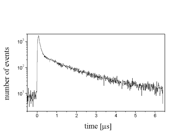
Figure 4: Time distributions of the 6.85 keV $\gamma$–quanta resulting from radiative de-excitation of the $d\mu{}^{3}\mathrm{He}$ complex obtained in coincidences with the muon decay electrons in run I.

The systematic error is larger than the uncertainty of the result caused by various possible model of the background, including the case where it is equal to zero (e.g., when time structure of the background is inaccurately known). We describe the procedure of determining $\lambda_{d{}^{3}\mathrm{He}}$ in more detail in Ref. Czapliński et al. (1996b).

IV.2 Number of muon stops in the $\mathrm{D}_{2}+{}^{3}\mathrm{He}$ mixture

The number of muon stops in the $\mathrm{D}_{2}+{}^{3}\mathrm{He}$ mixture was determined by analyzing time distributions of events detected by the four electron counters, We detailed this matter in Refs. Czapliński et al. (1996a); Boreiko et al. (1998); Bystritsky et al. (2003). Here it is pertinent to dwell upon some particular points in determination of this value.

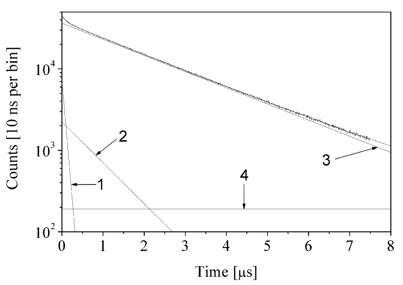
Figure 5: Time distributions of muon decay electrons measures in run I. The solid curves are the results of fitting its components (see Eq. (23)): 1 - Au; 2 - Al; 3 - $\mathrm{D}_{2}+{}^{3}\mathrm{He}$; 4 - constant background.

By way of example Fig. 5 shows the time distribution of muon decay electrons measured in run I. To determine the number of muon stops in the $d\mu{}^{3}\mathrm{He}$ the time distribution of the detected electrons, $dN_{e}/dt$, is approximated by an expression which is superposition of four exponents and a background of accidental coincidences

$$\frac{dN_{e}}{dt}=A_{\mathrm{Al}}^{e}e^{-\lambda_{\mathrm{Al}}t}+A_{\mathrm{Au}}^{e}e^{-\lambda_{\mathrm{Au}}t}+A_{\mathrm{He}}^{e}e^{-\lambda_{\mathrm{He}}t}+A_{\mathrm{D}}^{e}e^{-\lambda_{0}t}+B^{e},$$ (18)

where $A_{\mathrm{Al}}^{e}$, $A_{\mathrm{Au}}^{e}$, $A_{\mathrm{He}}^{e}$ and $A_{\mathrm{D}}^{e}$, are the normalized amplitudes with

$$A^{e}_{i}=N_{\mu}^{i}Q_{i}\lambda_{0}\varepsilon_{e}\qquad i=\mathrm{Al},\,\mathrm{Au},\,\mathrm{He},\,\mathrm{D},$$ (19)

and

$$\lambda_{\mathrm{Al}} = Q_{\mathrm{Al}}\cdot\lambda_{0}+\lambda_{\mathrm{cap}}^{\mathrm{Al}}\,,$$

$$\lambda_{\mathrm{Au}} = Q_{\mathrm{Au}}\cdot\lambda_{0}+\lambda_{\mathrm{cap}}^{\mathrm{Au}}\,,$$ (20)

$$\lambda_{\mathrm{He}} = \lambda_{0}+\lambda_{\mathrm{cap}}^{\mathrm{He}}\,,$$

are the muon disappearance rates in the different elements (the rates are the inverse of the muon lifetimes in the target wall materials). In reality, Eq. (18) is an approximation of a more complex equation, which can be found in Ref. Knowles (1999). The different rates are $\lambda_{0}=0.455\times 10^{6}\,\mbox{s}^{-1}$ and $\lambda_{cap}^{\mathrm{He}}=2216(70)\,\mbox{s}^{-1}$ Maev et al. (1996). The nuclear capture rates in aluminum and gold, $\lambda_{\mathrm{cap}}^{\mathrm{Al}}=0.7054(13)\times 10^{6}\,\mbox{s}^{-1}$ and $\lambda_{\mathrm{cap}}^{\mathrm{Au}}=13.07(28)\times 10^{6}\,\mbox{s}^{-1}$, are taken from Ref. Suzuki et al. (1987). $Q_{\mathrm{Al}}$ and $Q_{\mathrm{Au}}$ are the Huff factors, which take into account that muons are bound in the $1s$ state of the respective nuclei when they decay. This factor is negligible for helium but necessary for aluminum $Q_{\mathrm{Al}}=0.993$ and important for gold $Q_{\mathrm{Au}}=0.850$ Suzuki et al. (1987). The constant $B^{e}$ characterizes the random coincidence background.

We denote $N_{\mu}$ as the total number of muon stops in the target, $N_{\mu}^{\mathrm{Al}}$, $N_{\mu}^{\mathrm{Au}}$, and $N_{\mu}^{\mathrm{D/He}}$ as the numbers of muon stops in Al, Au, and the gaseous $\mathrm{D}_{2}+{}^{3}\mathrm{He}$ mixture, respectively. Thus, we have the relation

$$N_{\mu}=N_{\mu}^{\mathrm{Al}}+N_{\mu}^{\mathrm{Au}}+N_{\mu}^{\mathrm{D/He}}\,.$$ (22)

Since the muon decay with emission electrons in the $\mathrm{D}_{2}+{}^{3}\mathrm{He}$ mixture take place from the $1s$ state of the $d\mu$ or $\mu{}^{3}\mathrm{He}$ atom, the third and fourth terms in Eq(18) will differ only by the values of the amplitudes $A^{e}_{\mathrm{He}}$ and $A^{e}_{\mathrm{D}}$ because the slopes of both exponents are practically identical ($\lambda_{\mathrm{He}}=0.457\,\mu\mbox{s}^{-1}$, $\lambda_{0}=0.455\ \mu\mathrm{s}^{-1}$). In this connection the following simplified expression was used to approximate experimental time distributions of

$$\frac{dN_{e}}{dt}=A_{\mathrm{Al}}^{e}e^{-\lambda_{\mathrm{Al}}t}+A_{\mathrm{Au}}^{e}e^{-\lambda_{\mathrm{Au}}t}+A_{\mathrm{D/He}}^{e}e^{-\tilde{\lambda}_{\mathrm{D/He}}t}+B^{e},$$ (23)

Under our experimental conditions of runs I and II, we obtained the effective rates $\tilde{\lambda}_{D/He}=0.4563\,\mu\mbox{s}^{-1}$ and 0.4567 $\mu\mbox{s}^{-1}$, respectively. With these effective muon decay rates, the uncertainty in the calculated number of muon stops in the gaseous $\mathrm{D}_{2}+{}^{3}\mathrm{He}$ mixture is negligibly small as compared with the more rigorous calculation of this value by Eq. (18).

The amplitudes in Eq. (19) are expressed in terms of the factors $a_{Al}$, $a_{Au}$, and $a_{D/He}$, defined as the partial muon stopping in Al, Au, and $\mathrm{D}_{2}+{}^{3}\mathrm{He}$ mixture,

$$a_{i}=\frac{N_{\mu}^{i}}{N_{\mu}}\,,\qquad\sum_{i}a_{i}=1\,\qquad i=\mathrm{Al},\,\mathrm{Au},\,\mathrm{D/He}\,;$$ (24)

take the new form

$$A^{e}_{i}=N_{\mu}\lambda_{0}Q_{i}\varepsilon_{e}a_{i}\,.$$ (25)

The electron detection efficiency, $\varepsilon_{e}$, of the detectors E_UP, E_DO, E_RI and E_LE was determined as a ratio between the number of events belonging to the $K$–lines of the $\mu{}^{3}\mathrm{He}$ atoms, found from the analysis of the data with and without the del-$e$ criterion,

$$\varepsilon_{e}=\frac{N_{x-e}}{N_{x}}\,,$$ (26)

where $N_{x-e}$ and $N_{x}$ are the numbers of events belonging to $K$–lines of the $\mu{}^{3}\mathrm{He}$ atom and detected by the germanium detector with and without coincidence with the electron detectors. The thus measured experimental value is electron detection efficiency averaged over the target volume. Table 4 presents the results.

Table 4: Electron detection efficiencies, $\varepsilon_{e}$, in [%].

Run	Detector
	EUP	ERI	EDO	ELE	all
I	4.77(16)	5.69(16)	4.91(16)	0.169(24)	16.40(31)
II	4.53(15)	5.89(18)	4.88(14)	0.114(39)	16.34(39)
$\varepsilon_{e}$	4.65(12)	5.79(12)	4.89(12)	0.148(23)	16.37(22)

The electron detection efficiency of the detector E_LE is considerably lower than that of each of the other three electron detectors. This is because the material (Al, Fe) layer which the muon decay electron has to pass through in the direction of the detector E_LE is thicker than material layers in the direction of the other electron detectors.

Table 5 lists the values of the fraction of muons stopped in the $\mathrm{D}_{2}+{}^{3}\mathrm{He}$ mixture, $a_{D/He}$, found from the analysis of the time distributions of the events detected by the four electron detectors in runs I and II. Note that when the $a_{D/He}$ fraction, was calculated by Eqs. (24) and (25) it was assumed that the electron detection efficiency by each of the detectors E_UP, E_DO, E_RI and E_LE did not depend on the coordinates of the muon stop point in the target (be it in the target walls or in the $\mathrm{D}_{2}+{}^{3}\mathrm{He}$ mixture).

Table 5: Fraction of muons stopped in the gaseous deuterium-helium mixture found by the absolute method. $N_{\mu}^{D/He}$ is the number of muons stops in the $\mathrm{D}_{2}+{}^{3}\mathrm{He}$ gas mixture.

Run	$a_{D/He}$	$N_{\mu}^{D/He}$
	[%]	[$10^{9}$]
I	$47.5(6)_{stat}(30)_{syst}$	4.216
II	$66.6(10)_{stat}(39)_{syst}$	2.616

The systematic errors were determined as one half of the maximum spread between the $a_{D/He}$ values found from analysis of the time distributions of the electrons detected by each of the electron detectors E_UP, E_DO, E_RI and E_LE. Note that the fraction of muons stopped in gas, $a_{D/He}$, is a result of simultaneously fitting all time distributions obtained with each of the electron detectors (and not a result of averaging all four distributions corresponding to each of the four detectors).

IV.3 Determination of the detection efficiency for 14.64 MeV protons

To determine the proton detection efficiency, $\varepsilon_{p}$, of the three Si($dE-E$) telescopes, one should know the distribution of muon stops over the target volume in runs I and II. The average muon beam momentum $\overline{\mathrm{P}}_{\mu}$ corresponding to the maximum fraction $a_{D/He}$ of muons stopped in the $\mathrm{D}_{2}+{}^{3}\mathrm{He}$ mixture in runs I and II was found by varying the muon beam momentum $\overline{\mathrm{P}}_{\mu}$ and analyzing the time distributions of the detected electrons by Eq. (23). Next, knowing the average momentum $\overline{\mathrm{P}}_{\mu}$ and the beam momentum spread, we simulated the real distribution of muon stops in runs I and II by the Monte Carlo (MC) method Jacot-Guillarmod (1997). The results of the simulation were used in another Monte Carlo program to calculate the detection efficiency of each pair of Si($dE-E$) detectors for protons from reaction (2aa) Woźniak et al. (1996). The algorithm of the calculation program included simulation of the muon stop points in the $\mathrm{D}_{2}+{}^{3}\mathrm{He}$ mixture and the $d\mu$ and $\mu{}^{3}\mathrm{He}$ atom formation points, the consideration of the entire chain of processes occurring in the $\mathrm{D}_{2}+{}^{3}\mathrm{He}$ mixture from the instant when the muon hits the target to the instant of possible production of 14.64 MeV protons in the fusion reaction in the $d\mu{}^{3}\mathrm{He}$ complex. The calculation program took into account the proton energy loss in the gas target, kapton windows and Si($dE-E$) detectors themselves (in the thin Si($dE$) and thick Si($E$) detectors). The proton detection efficiency $\varepsilon_{p}$ was calculated at the $q_{1s}$, $W_{d}$, and $\lambda_{d\mu}$ values (see Table 3) corresponding to our experimental conditions. The scattering cross sections of $d\mu$ atoms form $\mathrm{D}_{2}$ molecules were taken from Refs. Chiccoli et al. (1992); Adamczak et al. (1996); Melezhik and Woźniak (1992).

We ceased tracing the muon stopped in the target when

• the muon decays ($\mu^{-}\to e^{-}+\nu_{\mu}+\tilde{\nu}_{e}$)

• the muon is transferred from the deuteron to the ${}^{3}\mathrm{He}$ nucleus with the formation of a ${}^{3}\mathrm{He}$$\mu$ atom

• nuclear fusion occurs in the $d\mu{}^{3}\mathrm{He}$ complex

• a $dd\mu\to p+t+\mu$ reaction proceeds in the $dd\mu$ molecule.

Note that the algorithm of the program also involved the consideration of the background process resulting from successive occurrence of the reactions

$$d\mu+d\rightarrow dd\mu\rightarrow\! \!{}^{3}\mathrm{He}\! \!(0.8\ \mathrm{MeV})+n$$ (27)

$$+$$

$$d\! \!\to\alpha+p(14.64\,\mathrm{MeV}).$$

This reaction (27) is called $d{}^{3}\mathrm{He}$ “fusion in flight”.

Figure 6: Cross section for the reaction ${}^{3}\mathrm{He}+d\to{}^{4}\mathrm{He}+p$ in flight (reaction (27)) as a function of the ${}^{3}\mathrm{He}$ nucleus-deuteron collision energy. The solid curve is the result of averaging the entire bulk of the presented experimental data.

In our calculations we used the dependence of the cross section for reaction (27) on the ${}^{3}\mathrm{He}$ deuteron collision energy, averaged over the data of Refs. White et al. (1997); Kunz (1955); Kljuchaiev et al. (1956); Allred et al. (1952); Argo et al. (1952); Freier and Holmgren (1954). Figure 6 displays the cross section dependence on the ${}^{3}\mathrm{He}$ deuteron collision energy. The program also took into account the energy loss of ${}^{3}\mathrm{He}$ nuclei in the $\mathrm{D}_{2}+{}^{3}\mathrm{He}$ mixture caused by ionization of ${}^{3}\mathrm{He}$ atoms and deuterium molecules. The time distributions of protons from reactions (2aa) and (27) under the same experimental conditions have completely different shapes in accordance with the kinetics of processes in the $\mathrm{D}_{2}+{}^{3}\mathrm{He}$ mixture.

Figure 7: Calculated time distributions of the protons form reactions (2aa) in runs I (left) and II (right).

Figure 8: Calculated time distributions of the protons form reactions (27) in runs I (left) and II (right).

Figures. 7 and  8 show the calculated time dependencies of the expected yields of protons from reactions (2aa) and (27) under the conditions of runs I and II. Thus, there arises a possibility of selecting a time interval of detection of events by the Si($dE-E$) detectors where the ratio of the reaction (2aa) and (27) yields is the largest. This, in turn, makes it possible to suppress the detected background from reaction (27) to a level low enough to meet the requirement of the experiment on the study of nuclear fusion in the $d\mu{}^{3}\mathrm{He}$ complex. Table 6 presents the calculated values of some quantities describing kinetics of muonic processes in the $\mathrm{D}_{2}+{}^{3}\mathrm{He}$ mixture and the process of detecting protons from reactions (2aa) and (27).

Table 6: Calculated values of the quantities describing kinetics of muonic processes in the $\mathrm{D}_{2}+{}^{3}\mathrm{He}$ mixture. The probabilities $W_{{}^{3}\mathrm{He}}$, $W_{d\mu{}^{3}\mathrm{He}}$, and $W_{d{}^{3}\mathrm{He}}$ are given per muon stop in the gaseous $\mathrm{D}_{2}+{}^{3}\mathrm{He}$ mixture.

Run	$W_{{}^{3}\mathrm{He}}$	$W_{d\mu{}^{3}\mathrm{He}}$	$W_{d{}^{3}\mathrm{He}}$	$W_{\mu e}$	$\varepsilon_{p}$	$\varepsilon_{p}^{ff}$	$\eta_{p}$	$\eta_{p}^{ff}$
	[$10^{-2}$]	[$10^{-1}$]	[$10^{-5}$]	[$10^{-1}$]	[$10^{-2}$]	[$10^{-2}$]	[$10^{-8}$]	[$10^{-8}$]
I	2.60	4.00	2.735	3.64	3.40	3.54	2.26	2.52
II	2.87	5.16	2.735	2.06	3.67	3.47	2.16	2.72

$W_{{}^{3}\mathrm{He}}$ is the total probability for the ${}^{3}\mathrm{He}$ formation ($E_{{}^{3}\mathrm{He}}=0.8$ MeV) in the $\mathrm{D}_{2}+{}^{3}\mathrm{He}$ mixture, as a result of the fusion reaction in the $dd\mu$ molecule. $W_{d\mu{}^{3}\mathrm{He}}$ is the $d\mu{}^{3}\mathrm{He}$ complex formation probability and $W_{d{}^{3}\mathrm{He}}$ is the probability for $d{}^{3}\mathrm{He}$ fusion in flight, following reaction (27), and $W_{\mu e}$ is the branching ratio of the muon decay via the $\mu^{-}\to e^{-}+\nu_{\mu}+\bar{\nu}_{e}$ channel. $\varepsilon_{p}$ and $\varepsilon_{p}^{ff}$ are the detection efficiencies of one Si($dE-E$) telescope for protons from reactions (2aa) and (27), respectively. $\eta_{p}$ and $\eta_{p}^{ff}$ are the yields of protons from reactions (2aa) and (27) detected by the Si($dE-E$) telescope per muon stop in the gaseous $\mathrm{D}_{2}+{}^{3}\mathrm{He}$ mixture (the value of $d\mu{}^{3}\mathrm{He}$ fusion rate $\lambda_{f}=10^{6}\,\mbox{s}^{-1}$ was used for calculation of $\eta_{p}$). There are some noteworthy intermediate results in the calculation of the detection efficiencies for protons from reactions (2aa) and (27). Table 7 presents average energy losses of protons on their passage through various material in the direction of the Si($dE-E$) detectors.

Table 7: Average energy losses, in MeV, of protons on their passage through various materials.

Run	$\mathrm{D}_{2}+{}^{3}\mathrm{He}$	kapton	Si($dE$)	Si($E$)
	gas	window
I	1.1	0.6	3.0	10.1
II	3.5	0.7	3.7	6.9

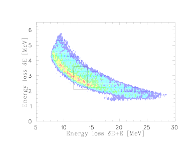
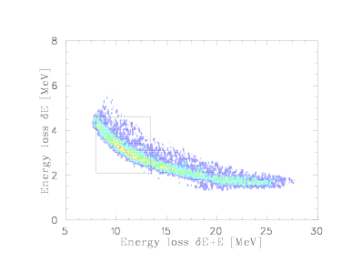
Figure 9: Two-dimensional distributions of events detected by the Si($dE-E$) telescopes in runs I (left) and II (right).

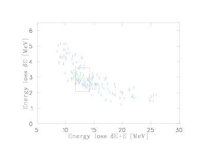
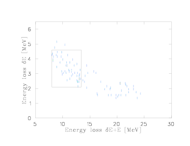
Figure 10: Two-dimensional distributions of events detected by the Si($dE-E$) telescopes in runs I (left) and II (right) with the del-$e$ coincidence.

Figures 9 show the two-dimensional distributions of events detected by the Si($dE-E$) detectors without coincidences with muon decay electrons in runs I and II. The x–axis represents the energy losses in the thin Si($dE$) counters and the y–axis shows the total energies losses by the particle in both the Si($dE$) and Si($E$) detectors connected in coincidence. The distributions of events in Figs. 9 correspond to the detection of protons arising both from reactions (2aa) and (27) and from the background reactions such as

$$\mu+{}^{3}\mathrm{He} \to p+2n+\nu_{\mu}$$

$$\mu+\mathrm{Al} \to\mathrm{Na}^{*} +p+n+\nu_{\mu}$$ (28)

$$+p+\nu_{\mu}$$

$$+p+2n+\nu_{\mu}$$

$$\mu+\mathrm{Fe} \to\mathrm{Cr}^{*} +p+n+\nu_{\mu}$$

$$+p+\nu_{\mu}$$

$$+p+2n+\nu_{\mu}\,.$$

In addition, the background which is not correlated with muon stops in the target (background of accidental coincidences) contributes to these distributions.

Figures 10 show the two-dimensional Si($dE-(E+dE)$) distributions obtained in coincidences with muon decay electrons. As seen, the use of the del-$e$ criterion leads to an appreciably reduction of the background, which in turn makes it possible to identify a rather weak effect against the intensive background signal. To suppress muon decay electrons in the Si($dE-E$) telescope, provision was made in the electronic logic of the experiment to connect each of the electron detectors in anti-coincidence with the corresponding Si($dE-E$) telescope. The choice of optimum criteria in the analysis of the data from the Si($dE-E$) telescopes was reduced to the determination of the boundaries and widths of the time and energy intervals where the background is substantially suppressed in absolute value and the effect-to-background ratio is the best. To this end the two-dimensional Si($dE-(dE+E)$) distributions corresponding to the detection of protons were simulated by MC method for runs I and II. On the basis of these distributions boundaries were determined for the energy interval of protons from reaction (2aa) where the loss of the “useful” event statistics collected by the Si telescope would be insignificant.

Figures 11 and 12 show the two-dimensional Si($dE-(dE+E)$) distributions corresponding to the proton detection which were simulated by the MC method for runs I and II. Based on these distributions, we chose some particular proton energy intervals named $\Delta E_{\Sigma}$ when considering the total energy deposited and $\delta E$ when looking only at the Si($dE$) detector (see Table 8) for further analysis. The regions of events corresponding to the intervals $\delta E$ and $\Delta E_{\Sigma}$ are shown in the form of rectangles on the two- dimensional distributions presented on the Fig. 9 and 10.

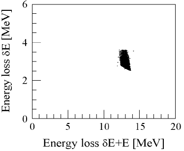
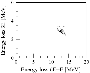
Figure 11: Two-dimensional distributions of Si($dE-(dE+E)$) events obtained in run I by the Monte Carlo method and corresponding to detection of protons from reactions (2aa) (left) and (27) (right) in the time interval $\Delta t_{\mathrm{Si}}$.

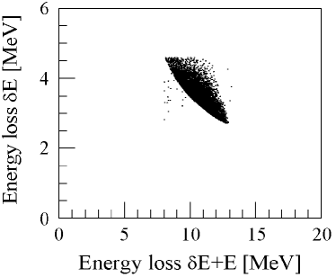
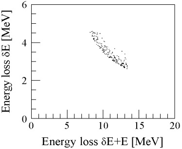
Figure 12: Two-dimensional distributions of Si($dE-(dE+E)$) events obtained in run II by the Monte Carlo method and corresponding to detection of protons from reactions (2aa) (left) and (27) (right) within the time interval $\Delta t_{\mathrm{Si}}$.

It is noteworthy that the proton detection efficiencies given in Table 6 correspond to these chosen proton energy intervals for runs I and II. The next step in the data analysis was to choose a particular times interval of detection of events by the Si($dE-E$) telescope. Figures 11 and 12 show the simulated time distributions of protons corresponding to the chosen energy loss intervals $\delta E$, for the energy loss in the Si($dE$) detector and $\Delta E_{\Sigma}=E+\delta E$ the energy loss in both silicon detector. For the chosen proton energy intervals Table 8 presents the statistics suppression factors corresponding to different initial time,$t_{thr}$ (with respect to the instant of the muon stop in the target) of the time intervals of detection of proton events. These factors correspond to the $\varepsilon_{Y}$ value in Eq. (11). The data in Table 8 are derived from time dependencies of the yields of protons from reactions (2aa) and (27) (see Figs. 7 and 8).

Table 8: Time factors for reaction (2aa) and reaction (27) for the chosen intervals of energies of protons detected by the Si($dE-E$) telescopes and detection beginning time, $t_{thr}$.

Run	$\Delta E_{\Sigma}$	$\delta E$	Reaction (2aa)					Reaction (27)
	[MeV]	[MeV]	$t_{thr},\ \mu\mathrm{s}^{-1}$					$t_{thr},\ \mu\mathrm{s}^{-1}$
			0.0	0.2	0.4	0.7	0.9	0.0	0.2	0.4	0.7	0.9
I	[$0-\infty$]	[$0-\infty$]	0.911	0.684	0.524	0.350	0.264	0.989	0.599	0.388	0.198	0.131
	[$11.7-14.2$]	[$2.1-3.6$]	0.878	0.659	0.505	0.337	0.254	0.438	0.263	0.171	0.090	0.058
II	[$0-\infty$]	[$0-\infty$]	0.934	0.543	0.316	0.129	0.059	0.996	0.333	0.114	0.025	0.009
	[$8.0-13.4$]	[$2.1-4.6$]	0.904	0.525	0.306	0.125	0.057	0.752	0.252	0.084	0.018	0.006

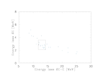
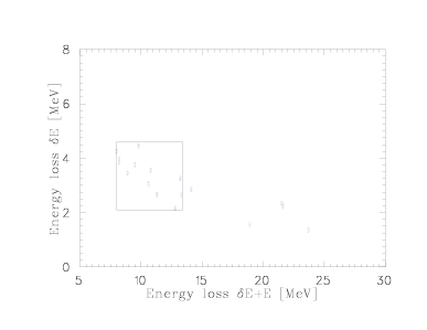
Figure 13: Two-dimensional distributions of events detected by the Si($dE-E$) telescopes in runs I (left) and II (right) with the del-$e$ coincidence and the time interval $\Delta t_{\mathrm{Si}}$ as define in Eq. (IV.3).

According to the data given in Table 8, we took the following time intervals $\Delta t_{\mathrm{Si}}$ (with $t_{\mathrm{Si}}$ the time for the Si signal to appear) for analyzing the events

$$\Delta t_{\mathrm{Si}}\,\mbox{(run I)}:\qquad 0.7\leq t_{\mathrm{Si}} \leq 2.2\,\mu\mbox{s}$$

$$\Delta t_{\mathrm{Si}}\,\mbox{(run II)}:\qquad 0.4\leq t_{\mathrm{Si}} \leq 1.2\,\mu\mbox{s}\,.$$ (29)

Figures 13 display the two-dimensional distributions of Si($dE-E$) events obtained in coincidences with muon decay electrons in runs I and II with this time criteria imposed. With these time intervals $\Delta t_{\mathrm{Si}}$ and the proton energy loss $\Delta E_{\Sigma}$ and $\delta E$ intervals, the statistics collection suppression factors for events from reactions (2aa) and (27) are

$$k_{d\mu{}^{3}\mathrm{He}}=2.9, k_{d{}^{3}\mathrm{He}} =11.2,\qquad\mbox{Run I,}$$

$$k_{d\mu{}^{3}\mathrm{He}}=3.2, k_{d{}^{3}\mathrm{He}} =12.1,\qquad\mbox{Run II.}$$

Another stage of the data analysis was the determination of the number of events detected by the Si($dE-E$) telescopes in runs I and II under the following criteria

• the coincidence of signals from the Si telescopes and electron detectors in the time interval $0.2<(t_{e}-t_{\mathrm{Si}})<5.5\,\mu$s ($t_{e}$ is the time when the E detector signal appear). Such a requirement add the efficiency factor $\varepsilon_{t}=0.83$ when determining the rates.

• the total energy release in the Si($dE$) detector is $\delta E$ as given in Table 8. This particular $\delta E$ interval will be called $\delta E$. For the thin and thick Si detector together, we choose the smallest interval, namely $\Delta E_{\Sigma}=[11.7-14.2]$ MeV for run I and $\Delta E_{\Sigma}=[8.0-13.4]$ MeV for run II.

• the time when the signal from the Si telescope appears falls in the $\Delta t_{\mathrm{Si}}$ intervals.

Table 9 presents the numbers of events $N_{p}$ detected in runs I and II under the above mentioned criteria.

Table 9: Numbers of detected events, $N_{p}$ and $N_{p}^{ff}$ for the chosen $\delta E$ and $\Delta E_{\Sigma}$ intervals, taking into account the time intervals $t_{e}-t_{\mathrm{Si}}$, and $\Delta t_{\mathrm{Si}}$. Also the accidental coincidence background, $N_{p}^{acc}$, as well as the total background, $N_{p}^{bckg}$.

Run	$N_{p}$	$N_{p}^{ff}$	$\eta_{Si-E}$	$N_{p}^{acc}$	$N_{p}^{bckg}$
			[$10^{-4}$]
I	14	3.8(2)	4.2(9)	2.5(5)	6.3(6)
II	11	2.4(1)	2.4 (11)	1.1(5)	3.5(5)

The contribution of the background events, $N_{p}^{ff}$, given in Table 9 from the reaction (27) is found in the following way. The expected number of detected protons from reaction (27) in runs I and II is calculated by

$$N_{p}^{ff}=\frac{N_{\mu}a_{D/He}W_{{}^{3}\mathrm{He}}W_{d{}^{3}\mathrm{He}}\varepsilon^{ff}_{p}N_{\mathrm{Si}}\varepsilon_{e}\varepsilon_{t}}{k_{d{}^{3}\mathrm{He}}}\,.$$ (31)

$N_{\mathrm{Si}}$ is the number of Si($dE-E$) telescopes and $1/{k_{d{}^{3}\mathrm{He}}}$ is the factor of background suppression by imposing the criteria (ii) and (iii). Using the values of $a_{D/He}$ and $N_{\mu}$ measured in runs I and II, the calculated values of $W_{{}^{3}He}$, $W_{d^{3}He}$, $\varepsilon^{f}_{p}$, $N_{\mathrm{Si}}$, $k_{d{}^{3}\mathrm{He}}$, $\varepsilon_{t}$, and Eq. (31), we obtained $N_{p}^{ff}$, which is given in Table 9. Errors of the calculated $N_{p}^{ff}$ arose from the inaccurate dependence of the cross sections $\sigma_{d{}^{3}\mathrm{He}}$ for the $d{}^{3}\mathrm{He}$ reaction in flight on the ${}^{3}\mathrm{He}$ deuteron collision energy and from the errors in the calculations of the detection efficiency of the Si telescopes for protons from reaction (27). These errors were found by substituting various experimental $\sigma_{d^{3}He}(E_{d^{3}He})$ dependencies White et al. (1997); Kunz (1955); Kljuchaiev et al. (1956); Allred et al. (1952); Argo et al. (1952); Freier and Holmgren (1954). into the program for Monte Carlo calculation of the in-flight $d{}^{3}\mathrm{He}$ fusion probability $W_{d{}^{3}\mathrm{He}}$.

Now it is necessary to find the level of the accidental coincidence background by analyzing the experimental data from runs I and II. To this end the two-dimensional distribution of events detected by the Si($dE-E$) telescopes was divided into three regions which did not include the separated region of events belonging to the process (2aa). Considering the boundaries of the intervals $\delta E$ and $\Delta E_{\Sigma}$ of energy losses of the protons from reaction (2aa) we used three regions, A,B, and C, of the two-dimensional $\delta E-\Delta E_{\Sigma}$ distributions for determining the background level. The regions are given in Table 10.

The level $N_{p}^{acc}$ of the background of the accidental coincidences of signals from the Si($dE-E$) telescopes and the electron detectors for the given three region of the two-dimensional $\delta E-\Delta E_{\Sigma}$ distributions and the corresponding suppression factor of the accidental background in the Si telescopes, $\eta_{Si-E}$, are defined as

$$N_{p}^{acc}=N^{f}_{\mathrm{Si}}\eta_{Si-E},$$ (32)

$$\eta_{Si-E}=\frac{\sum\limits_{i}N^{i}_{Si-E}}{\sum\limits_{i}N^{i}_{Si}},$$ (33)

where $N^{f}_{\mathrm{Si}}$ is the number of events detected by the three Si($dE-E$) telescopes and belonging to the selected $(\delta E-\Delta E_{\Sigma})$ region of detection of protons from reaction (2aa). $N^{i}_{Si-E}$ and $N^{i}_{Si}$ are the numbers of events detected by the $i$th Si($dE-E$) telescope with and without del-$e$ coincidences and belonging to the other $(\delta E-\Delta E_{\Sigma})$ intervals. Note that the degree of suppression of the accidental coincidence background was determined not only by averaging the data obtained with the $\mathrm{D}_{2}+{}^{3}\mathrm{He}$ mixture but also in additional experiments with the targets filled with pure ${}^{4}\mathrm{He}$, $\mathrm{D}_{2}$, and ${}^{3}\mathrm{He}$ whose densities were $\varphi\approx 0.17$, $\varphi\approx 0.09$, and $\varphi\approx 0.035$,respectively. This guaranteed an identical ratio of stops in the target walls and in the gas in the experiments with ${}^{4}\mathrm{He}$, $\mathrm{D}_{2}$, and the $\mathrm{D}_{2}+{}^{3}\mathrm{He}$ mixture ($\varphi=0.168$) and in the experiments with the $\mathrm{D}_{2}+{}^{3}\mathrm{He}$ mixture ($\varphi=0.0585$) and ${}^{3}\mathrm{He}$. Figures 14, 15, and 16 display the two-dimensional distributions of background events detected by the Si($dE-E$) telescopes in the experiments with ${}^{4}\mathrm{He}$, $\mathrm{D}_{2}$, and ${}^{3}\mathrm{He}$.

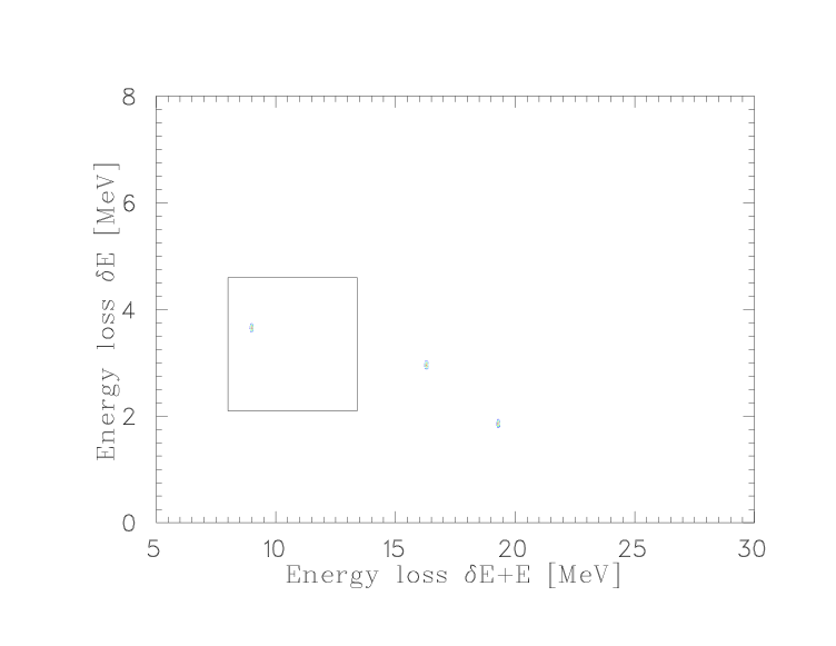
Figure 14: Two-dimensional distributions of events detected by the Si($dE-E$) telescopes in a run with pure deuterium with the del-$e$ coincidences and within the $\Delta t_{\mathrm{Si}}$ interval. The rectangle is the region corresponding to the energy intervals $\delta E$ and $\Delta E_{\Sigma}$ for the run with the $\mathrm{D}_{2}+{}^{3}\mathrm{He}$ mixture at $\varphi=0.168$.

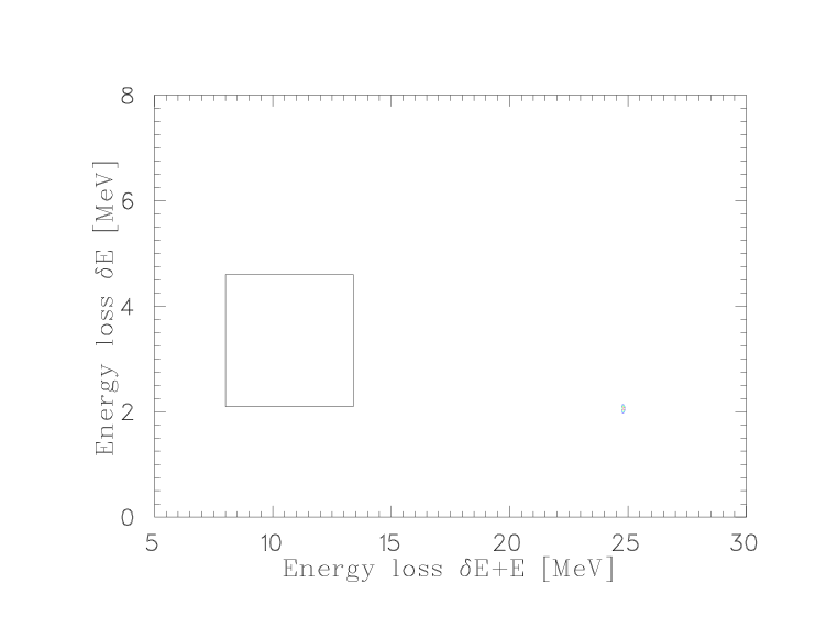
Figure 15: Two-dimensional distributions of events detected by the Si($dE-E$) telescopes in the pure ${}^{4}\mathrm{He}$ with the del-$e$ coincidences and within the $\Delta t_{\mathrm{Si}}$ interval. The rectangle is region corresponding to the energy intervals $\delta E$ and $\Delta E_{\Sigma}$ for the run with the $\mathrm{D}_{2}+{}^{3}\mathrm{He}$ mixture at $\varphi=0.168$.

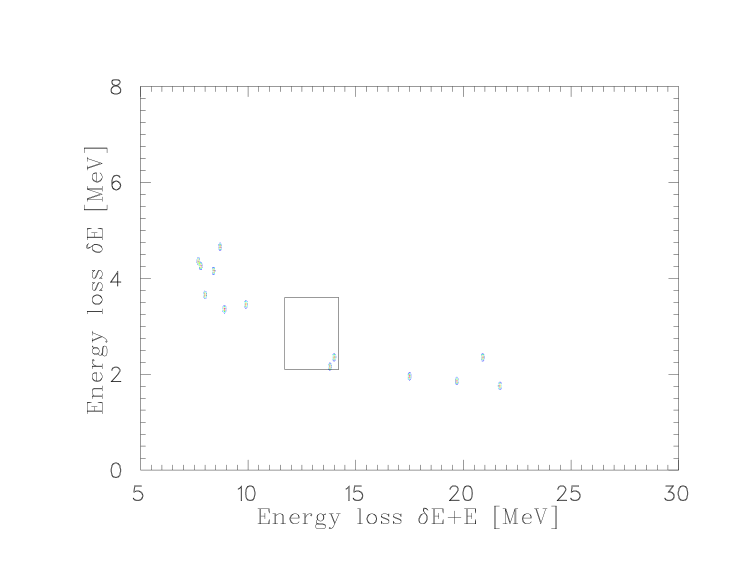
Figure 16: Two-dimensional distributions of events detected by the Si($dE-E$) telescopes in the run with pure ${}^{3}\mathrm{He}$ with the del-$e$ coincidence and within the $\Delta t_{\mathrm{Si}}$ interval. The rectangle is region corresponding to the energy intervals $\delta E$ and $\Delta E_{\Sigma}$ for the run with the $\mathrm{D}_{2}+{}^{3}\mathrm{He}$ mixture at $\varphi=0.0585$.

Table 10: The three regions of division of two-dimensional ($\delta E-\Delta E_{\Sigma}$) distributions. All energies are given in MeV.

	Region A		Region B		Region C
Run	$\Delta E_{\Sigma}$	$\delta E$	$\Delta E_{\Sigma}$	$\delta E$	$\Delta E_{\Sigma}$	$\delta E$
I	$0-11.7$	$3.6-6$	$0-11.7$	$0-3.6$	$14.2-25$	$1.8-6$
II	$0-8$	$4.6-6$	$0-8$	$0-4.6$	$13.6-25$	$1.5-6$

The values of $\eta_{Si-E}$ and $N_{p}^{acc}$ are given in Table 9 for runs I and II. The total numbers of detected background events,$N_{p}^{bckg}$, which belongs to the analyzed region of energies $(\delta E-\Delta E_{\Sigma})$ of protons from reaction (2aa) and met the criteria (i)–(iii) were defined as

$$N_{p}^{bckg}=N_{p}^{ff}+N_{p}^{acc}$$ (34)

and are also given in Table 9. The uncertainties of $N_{p}^{bckg}$ include both statistical and systematical errors.

Based on the measured values $N_{p}$ and the calculated values $N_{p}^{bckg}$ and following Refs. Helene (1984, 1983); Feldman and Cousins (1998), we found the yields of detected protons ,$Y_{p}$, from reaction (2aa) in runs I and II.

$$Y_{p} = 7.7^{+4.4}_{-3.4}\qquad\mbox{run I}$$

$$Y_{p} = 7.5^{+3.8}_{-3.2}\qquad\mbox{run II}$$ (35)

The errors of $Y_{p}$ are found in accordance with Refs. Helene (1984, 1983); Feldman and Cousins (1998) dealing with analysis of small statistical samples. In view of Eq. (11) and the measured values $Y_{p}$, the effective rate of nuclear fusion in the $d\mu{}^{3}\mathrm{He}$ complex is obtained from Eq. (15). It can be written as

$$\tilde{\lambda}_{f}=\frac{\lambda_{d\mu}\lambda_{\Sigma}}{N_{\mu}a_{D/He}W_{d}\,q_{1s}\,\varphi\,\mathrm{c}_{{}^{3}\mathrm{He}}\lambda_{d{}^{3}\mathrm{He}}}\frac{Y_{p}}{\varepsilon_{p}\,\varepsilon_{e}\,\varepsilon_{t}\varepsilon_{Y}}\,,$$ (36)

The values of $\tilde{\lambda}_{f}$ and $\lambda_{\Sigma}$ corresponding to the conditions of runs I and II are given in Table 11. Using Eq. (13) and the measured effective rates of nuclear fusion and assuming that $\lambda^{1}_{f}\ll\lambda^{0}_{f}$ Bogdanova et al. (1999), one can get hypothetical estimates of the partial fusion rate in the $d\mu{}^{3}\mathrm{He}$ complex in its states with the total orbital momentum $J=0$

$$\lambda^{J=0}_{f}=\frac{\tilde{\lambda}_{f}(\tilde{\lambda}_{10}+\lambda_{\Sigma}^{0})}{\tilde{\lambda}_{10}}.$$ (37)

Table 11 also presents the values for $\lambda^{J=0}_{f}$ found in runs I and II.

Table 11: Effective rates of the $1\to 0$ transition, $\tilde{\lambda}_{10}$, and the nuclear fusion rates in the $d\mu{}^{3}\mathrm{He}$ complex.

Run	$\tilde{\lambda}_{10}$	$\lambda^{J=0}_{f}$	$\tilde{\lambda}_{f}$	$\lambda_{\Sigma}$
	[ $10^{11}\,\mbox{s}^{-1}$ ]	[ $10^{5}\,\mbox{s}^{-1}$ ]	[ $10^{5}\,\mbox{s}^{-1}$]	[ $10^{11}\,\mbox{s}^{-1}$ ]
I	5.2	$9.7^{+5.7}_{-2.6}$	$4.5^{+2.6}_{-2.0}$	6.54
II	7.5	$12.4^{+6.5}_{-5.4}$	$6.9^{+3.6}_{-3.0}$	6.44

The averages $\lambda_{\Sigma}^{0}=6\times 10^{11}\,\mbox{s}^{-1}$ and $\lambda_{\Sigma}^{1}=7\times 10^{11}\,\mbox{s}^{-1}$ (averaging over the data Kino and Kamimura (1993); Gershtein and Gusev (1993); Czapliński et al. (1997b); Belyaev et al. (1995); Czapliński et al. (1996a); Belyaev et al. (1997); Czapliński et al. (1996b)) were used to get the values presented in Table 11. As to the effective rate for transition of the $d\mu{}^{3}\mathrm{He}$ complex from the state with the angular momentum $J=1$ to the state with $J=0$, it was calculated with allowance for the entire complicated branched chain of processes accompanying and competing with the rotational $1-0$ transition (see Table 11). The chain of these processes is considered in detail in Refs. Bogdanova et al. (1998); Bystritsky and Pen’kov (1999); Bystritsky et al. (1999b, c). The effective rates of nuclear fusion in the $d\mu{}^{3}\mathrm{He}$ complex found by us in runs I and II coincide within the measurement errors. This is also true for the $d{}^{3}\mathrm{He}$ fusion rates $\lambda^{J=0}_{f}$ obtained by Eq. (37). A comparison of the measured $\lambda^{J=0}_{f}$ with the theoretical calculations show rather good agreement with Czapliński et al. (1996b), a slight discrepancy with Refs. Pen’kov (1997); Bogdanova et al. (1999) and considerable disagreement with Refs. Nagamine et al. (1989); Harley et al. (1989). The cause of this disagreement is not clear yet as also is not clear the discrepancy between $\lambda^{J=0}_{f}$ calculations in Refs. Nagamine et al. (1989); Pen’kov (1997); Czapliński et al. (1996b); Harley et al. (1989) (see Table 1). Note that the theoretical papers Refs. Nagamine et al. (1989); Pen’kov (1997); Czapliński et al. (1996b); Harley et al. (1989); Bogdanova et al. (1999) yield estimates with a different degree of approximation. A correct comparison of the experimental and theoretical $\lambda^{J=0}_{f}$ is possible only after carrying out some experiments with the $\mathrm{D}_{2}+{}^{3}\mathrm{He}$ mixture ruling out model dependence on the effective rate of transition of the $d\mu{}^{3}\mathrm{He}$ complex from the $J=1$ state to the $J=0$ state.

A comparison of the results of this paper with the experimental results Maev et al. (1999) reveals appreciable disagreement between them. The shortened form of presentation of the results Maev et al. (1999) does not allow us to find out sufficiently well the cause of this considerable disagreement. Note, however, some results of the intermediate calculations which, to our mind, disagree with the real estimates of the calculated quantities.

1. According to Ref. Maev et al. (1999), the fraction of the $d\mu$ atoms which were formed in the excited state under their experimental conditions and came to the ground state (per muon stop in the target) is $C_{d\mu}=0.8$. The quantity $C_{d\mu}$ is defined as

   $$C_{d\mu}=\frac{1}{2}W_{p,d}(q^{p\mu}_{1s}+q^{d\mu}_{1s}),$$ (38)

   where $W_{p,d}$ is the probability for direct muon capture by the HD molecule followed by formation of the muonic hydrogen atom or the excited $d\mu$ atom. $q^{p\mu}_{1s}$ and $q^{d\mu}_{1s}$ are the probabilities for the transition of the $p\mu$ and $d\mu$ atoms from the excited state to the $1s$ ground state. According to Refs. Tresch et al. (1998b); Gartner et al. (2000); Bystritsky et al. (2004); Tresch et al. (1999), under the Maev et. al experimental conditions the values of the quantities appearing in Eq. (38) were $W_{p,d}=0.92$ $q^{p\mu}_{1s}=0.5$, and $q^{d\mu}_{1s}=0.8$. Thus, as follows from our estimation, $C_{d\mu}=0.6$ and not 0.8 as stated.

2. The number of $d\mu{}^{3}\mathrm{He}$ complexes formed in the course of data taking in their experiment was defined as

   $$N_{d\mu{}^{3}\mathrm{He}}=N_{\mu}C_{d\mu}\frac{\lambda_{d\mu{}^{3}\mathrm{He}}}{\lambda_{d\mu}}\,,$$ (39)

   and correspond to $N_{d\mu{}^{3}\mathrm{He}}=(4.9\pm 0.4)\times 10^{8}$.

   According to our estimations, the quantities $\lambda_{d\mu{}^{3}\mathrm{He}}$, $\lambda_{d\mu}$, $\lambda_{pd\mu}$ ($pd\mu$ molecule formation rate), and $N_{d\mu{}^{3}\mathrm{He}}$ had the values $\lambda_{d\mu{}^{3}\mathrm{He}}=1.32\times 10^{6}\ \mathrm{s}^{-1}$ ($\varphi=0.0975$ $\mathrm{c}_{{}^{3}\mathrm{He}}$ = 0.056, $\lambda^{0}_{d^{3}He}=2.42\times 10^{8}\ \mathrm{s}^{-1}$) Bystritsky et al. (2004),

   $$\lambda_{d\mu} \approx \lambda_{0}+\lambda_{d\mu{}^{3}\mathrm{He}}\varphi\mathrm{c}_{{}^{3}\mathrm{He}}+\lambda_{pd\mu}\varphi\mathrm{c}_{p}+\tilde{\lambda}_{F}\omega_{d}\varphi\mathrm{c}_{d}$$ (40)

   $$\approx 2.05\times 10^{6}\ \mathrm{s}^{-1}$$

   $\lambda_{pd\mu}=5.6\times 10^{6}\,\mathrm{s}^{-1}$, which yields $N_{d\mu{}^{3}\mathrm{He}}\approx 3.7\times 10^{8}\,\mbox{s}^{-1}$ instead of $(4.9\pm 0.4)\times 10^{8}\,\mbox{s}^{-1}$.

3. Their ionization chamber detection efficiency for protons from reaction (2aa) was defined as $\varepsilon=\varepsilon_{S}\varepsilon_{\tau}$ and found to be $\varepsilon=0.082$, where $\varepsilon_{S}=0.13$ is the selection factor for events detected in compliance with certain amplitude and geometrical criteria, $\varepsilon_{\tau}=0.63$ is the time factor to take of the fact that the detected events were analyzed in the time interval $0.4\leq t\leq 1.8\,\mu$s. According to our estimation, $\varepsilon_{\tau}=e^{-\lambda_{d\mu}t_{1}}-e^{-\lambda_{d\mu}t_{2}}=0.44$, because under their experimental conditions the $d\mu$ disappearance rate is $\lambda_{d\mu}\approx 2.05\times 10^{6}\,\mbox{s}^{-1}$, $t_{1}=0.4\,\mu$s, and $t_{2}=1.8\,\mu$s.

As can be seen, taking into account only the above items alone the upper limit of $\tilde{\lambda}_{f}$ is, to our mind, appreciably underestimated in the work of Maev et. al. Another cause of this underestimation might be the improper background subtraction procedure because they determined the background level using information from earlier experiments Balin et al. (1998) carried out under different conditions and at an experimental facility which was not completely analogous. In addition, it is slightly surprising that the background from muon capture by ${}^{3}\mathrm{He}$ nuclei with the formation of protons in the energy region near 14.64 MeV is estimated at zero in Ref. Maev et al. (1999)(see ).

We believe that our $\tilde{\lambda}_{f}$ measurement results are reliable, which is confirmed by stable observation of nuclear fusion in both runs with the $\mathrm{D}_{2}+{}^{3}\mathrm{He}$ mixture differing in density by a factor of about three. Nevertheless, as far as the experimental results obtained in this paper and in Ref. Maev et al. (1999) are concerned, the things are unfortunately uncertain and need clarifying.

There is a point important for comparison of the calculated $\lambda^{J=0}_{f}$ with the results of the previous experiments Maev et al. (1999) and this paper. Measurement of $\lambda^{J=0}_{f}$ is indirect because it is determined by Eq. (37) with the calculated effective rate for transition of the $d\mu{}^{3}\mathrm{He}$ complex from the $J=1$ state to the $J=0$ state. Therefore, $\lambda^{J=0}_{f}$ is not uniquely defined and greatly depends on $\tilde{\lambda}_{10}$, which in turn is determined by the chain of processes accompanying and competing with the $1-0$ transition of the $d\mu{}^{3}\mathrm{He}$ complex. To rule out this lack of uniqueness in determination of $\lambda^{J=0}_{f}$ and, in addition, to gain information on the effective $1-0$ transition rate $\tilde{\lambda}_{10}$ and the nuclear fusion rate $\lambda^{J=1}_{f}$ in the $d\mu{}^{3}\mathrm{He}$ complex in the $J=1$ state, it is necessary, as proposed in Refs. Bystritsky and Pen’kov (1999); Bystritsky et al. (1999b, c), to carry out an experiment with the $\mathrm{D}_{2}+{}^{3}\mathrm{He}$ mixture at least at three densities in the range $\varphi=0.03-0.2$, where not only protons from reaction (2aa) but also 6.85 keV $\gamma$ rays should be analyzed. Analysis of the results reported in this paper and in Ref. Maev et al. (1999) makes it possible to put forward some already obvious proposals as to getting unambiguous and precise information on important characteristics of $\mu$-molecular ($\lambda_{d\mu{}^{3}\mathrm{He}}$, $\tilde{\lambda}_{10}$) and nuclear ($\tilde{\lambda}_{f}$, $\lambda^{J=0}_{f}$, $\lambda^{J=1}_{f}$) processes occurring in the $\mathrm{D}_{2}+{}^{3}\mathrm{He}$ mixture. It is necessary to conduct experiments at no less than three densities of the ($\mathrm{HD}+{}^{3}\mathrm{He}$) or ($\mathrm{H}_{2}+\mathrm{D}_{3}(1\%)+{}^{3}\mathrm{He}$) mixture with detection of both protons from reaction (2aa) and 6.85 keV $\gamma$ rays, to increase at least three times the detection efficiency for protons $\varepsilon_{p}$ and for muon decay electrons $\varepsilon_{e}$ in comparison with the corresponding efficiencies in the present experiment.