Femtoscopy in Relativistic Heavy Ion Collisions: Two Decades of Progress

Abstract

Analyses of two-particle correlations have provided the chief means for determining spatio-temporal characteristics of relativistic heavy ion collisions. We discuss the theoretical formalism behind these studies and the experimental methods used in carrying them out. Recent results from RHIC are put into context in a systematic review of correlation measurements performed over the past two decades. The current understanding of these results is discussed in terms of model comparisons and overall trends.

1 Introduction

The study of nucleus-nucleus collisions at ultra-relativistic energies aims to characterize the dynamical processes by which matter at extreme densities is produced and the fundamental properties that this matter exhibits. In nucleus-nucleus collisions, how do partonic equilibration processes proceed? For how long, over which spatial extension, and at which density is a QCD equilibration state approached, and what are its properties? Particle densities attained during a heavy ion collision are expected to exceed significantly the inverse volume of a hadron. This implies that the high temperature phase of QCD, the Quark Gluon Plasma, comes within experimental reach. Chiral symmetry restoration and deconfinement phase transition are testable in heavy ion collisions. However, the experimental study of QCD at high temperatures and densities is complicated by the short lifetime and mesoscopic extension of the produced system. Femtoscopy, the spatio-temporal characterization of the collision region on the femtometer scale, is needed to frame any discussion of dynamical equilibration processes.

The Relativistic Heavy Ion Collider (RHIC) just completed the first part of a dedicated experimental heavy ion program. Center of mass energies ($\sqrt{s_{NN}}=200$ GeV) exceeded those of previous fixed target experiments by a factor 10. The current discussion of RHIC data focuses mainly on several qualitatively novel phenomena that all support the picture that dense and rapidly equilibrating QCD matter is produced in the collision region Adams:2005dq ; Adcox:2004mh ; Back:2004je ; Arsene:2004fa . In particular, identified single inclusive hadron spectra appear to emerge from a common flow field whose size and dependence on transverse momentum and azimuth is consistent with expectations that the produced matter is a locally equilibrated, almost ideal fluid of very small viscosity. Moreover, high-$p_{T}$ hadron spectra show a centrality dependent, strong suppression in Au+Au collisions, but not in a d+Au control experiment, indicating that even the hardest partons produced in the collision participate significantly in equilibration processes. In short, experiments at RHIC have demonstrated already that heavy ion collisions produce dense and equilibrating matter, and that controlled experimentation of this matter is possible using a large variety of probes.

Despite these successes, numerous questions remain concerning the state of the matter produced in these collisions. Most notably, the equation of state is far from being determined, and issues concerning chiral symmetry restoration are largely unresolved. Addressing these fundamental questions about bulk matter requires a detailed understanding of the dynamics and chemistry of the collision, which can only be acquired by thorough and coordinated analyses of data and theory. In particular, spatio-temporal aspects of the reaction need to be experimentally addressed. The small size, $\sim 10^{-14}$ m, and transient nature, $\sim 10^{-22}$ seconds, of the reactions preclude direct measurement of times or positions. Instead, femtoscopy must exploit measurements of asymptotic momenta. Correlations of two final-state particles at small relative momentum provide the most direct link to the size and lifetime of subatomic reactions Boal:1990yh ; Bauer:1993wq ; Heinz:1999rw ; Wiedemann:1999qn ; Csorgo:1999sj ; Weiner:1999th ; Tomasik:2002rx ; Alexander:2003ug . Because correlations from either interactions or from identity interference are stronger for smaller separations in space-time, spatio-temporal information can be most easily extracted for small sources, unlike the limitations of microscopes and telescopes.

The interference of two particles emitted from chaotic sources was first applied by Hanbury-Brown and Twiss HBT1 ; HBT2 , where photons were exploited to determine source sizes for both laboratory and stellar sources in the 1950s and 1960s. Correlations of identical pions were shown to be sensitive to source dimensions in proton-antiproton collisions by Goldhaber, Goldhaber, Lee, and Pais in 1960 Goldhaber:1960sf . In the 1970s, these methods were refined by Kopylov and Podgoretsky Kopylov:1972qw ; Kopylov:1974uc ; Kopylov:1974a ; Kopylov:1974b , Koonin, Koonin:1977fh , and Gyulassy Gyulassy:1979yi , and other classes of correlations were shown to be useful for source-size measurements, such as strong and Coulomb interactions. Bevalac analyses showed that interferometry was truly capable of quantitatively determining spatial and temporal source dimensions Zajc:1984vb ; Fung:1978 and providing a stringent test of dynamical models Humanic:1985qx . Throughout the last 25 years this phenomenology has developed into a precision tool for heavy ion collisions. Whereas hadronic sources are short lived and one measures correlations of the momentum of outgoing particles, stars are long lived and require experimental filters to enforce the approximate simultaneity of the two photons. Although the theory for these two classes of measurement are very different Baym:1997ce ; Kopylov:1976 , the heavy-ion community often uses the term HBT, in reference to Hanbury-Brown and Twiss’s original work with photons, to refer to any type of analysis related to size and shape that uses two particles at small relative momentum. To some, however, the term HBT refers only to identical-particle interferometry. Following Lednicky, we will employ the term femtoscopy Lednicky:1990pu ; Lednicky:2002fq to denote any measurement that provides spatio-temporal information, including coalescence analyses.

Femtoscopic measurements from truly relativistic heavy ion collisions were first reported almost twenty years ago. Since then, measurements have been performed for collisions at energies spanning two orders of magnitude. In a double sense, then, this review examines recent RHIC results within the larger context of two decades’ worth of femtoscopy. The theory and phenomenology of correlation femtoscopy are reviewed in the next section, with particular emphasis on describing the approximations used to derive the connection between spatio-temporal aspects of the emission function and correlations constructed from final-state momenta. Experimental methods and techniques are correspondingly reviewed in Section 3. Section 4 presents experimental results, with an emphasis on describing the systematics of source dimensions and lifetimes as a function of beam energy, system size, particle species and a particle’s momentum. In addition to source dimensions, results for phase space density and entropy are presented. Comparisons of experimental results and transport models are presented in Section 5, with an emphasis on explaining the “HBT puzzle,” i.e., the fact that dynamic descriptions that incorporate a phase transition to a new state of matter with many degrees of freedom significantly over-predict observed source sizes. Section 6 summarizes the current state of the field and lists new directions and challenges for future theoretical and experimental analyses.

2 Theory and Phenomenology Basics

2.1 Formalism

Two-particle correlation functions are constructed as the ratio of the measured two-particle inclusive and single-particle inclusive spectra,

$$C^{ab}({\bf P},{\bf q}) = \frac{dN^{ab}/(d^{3}p_{a}d^{3}p_{b})}{(dN^{a}/d^{3}p_{a})(dN^{b}/d^{3}p_{b})}\,,$$ (1)

$$P \equiv p_{a}+p_{b},~{}~{}q^{\mu}=\frac{(p_{a}-p_{b})^{\mu}}{2}-\frac{(p_{a}-p_{b})\cdot P}{2P^{2}}P^{\mu}\,.$$

The theoretical analysis of (1) aims at relating this experimentally measured correlation to the space-time structure of the particle emitting source Heinz:1999rw ; Bauer:1993wq ; Wiedemann:1999qn ; Tomasik:2002rx . Two forms are common for connecting the measured correlation function to the space-time emission function $s(p,x)$ through a convolution with the wave function $\phi$. In the first form Lednicky:1981su ,

$$C^{ab}({\bf P},{\bf q})=\frac{\int d^{4}x_{a}d^{4}x_{b}s_{a}(p_{a},x_{a})s_{b}(p_{b},x_{b})|\phi({\bf q}^{\prime},{\bf r}^{\prime})|^{2}}{\int d^{4}x_{a}s_{a}(p_{a},x_{a})\int d^{4}x_{b}s_{b}(p_{b},x_{b})}\,.$$ (2)

In calculations of two-particle correlation functions, the squared relative two-particle wave function $|\phi|^{2}$ serves generally as a weight, and the emission function $s(p,x)$ contains all space-time information about the source because it describes the probability of emitting a particle with momentum $p$ from a space-time point $x$. Here, and throughout this section, primes denote quantities in the center-of-mass frame, i.e., the frame where ${\bf P}=0$. The source function $s_{a}$ is evaluated at the momentum $\bar{{\bf p}}_{a}=m_{a}{\bf P}/(m_{a}+m_{b})$, $\bar{p}_{a}^{0}=E_{a}(\bar{\bf p}_{a})$.

The second form, which is equally justified as Equation 2 by the approximations described further below, is,

$$C^{ab}({\bf P},{\bf q})-1 = \int d^{3}r^{\prime}{\cal S}_{\bf P}({\bf r}^{\prime})\left[|\phi({\bf q}^{\prime},{\bf r}^{\prime})|^{2}-1\right],$$ (3)

$${\cal S}_{\bf P}({\bf r}^{\prime}) \equiv \frac{\int d^{4}x_{a}d^{4}x_{b}s_{a}(\bar{p}_{a},x_{a})s_{b}(\bar{p}_{b},x_{b})\delta\left({\bf r}^{\prime}-{\bf x}_{a}^{\prime}+{\bf x}_{b}^{\prime}\right)}{\int d^{4}x_{a}d^{4}x_{b}s_{a}(\bar{p}_{a},x_{a})s_{b}(\bar{p_{b}},x_{b})}~{}.$$

This expression allows one to consider $|\phi|^{2}$ as a kernel with which one can transform from the coordinate-space basis to the relative-momentum basis. It also emphasizes the limitation of correlation functions, that they can provide, at best, the function ${\mathcal{S}}_{\bf P}({\bf r}^{\prime})$, the distribution of relative positions of particles with identical velocities and total momentum ${\bf P}$ as they move in their asymptotic state. Thus, correlations do not measure the size of the entire source. Instead, they address the dimensions of the “region of homogeneity,” a term coined by Sinyukov Akkelin:1995gh , i.e., the size and shape of the phase space cloud of outgoing particles whose velocities have a specific magnitude and direction. If the collective expansion of the produced matter is strong, as is the case in central collisions, then the region of homogeneity is significantly smaller than the entire source volume. In the following, we discuss the assumptions on which Equations 2 and 3 are based.

We start from explicit expressions for the one- and two-particle spectra in terms of $T$-matrix elements. For one-particle emission,

$$E\frac{dN}{d^{3}p} = \int d^{4}x~{}s(p,x)=\sum_{F^{\prime}}|\int d^{4}xT_{F^{\prime}}(x)e^{-ip\cdot x}|^{2},$$ (4)

$$s(p,x) = \sum_{F^{\prime}}\int d^{4}\delta xT_{F^{\prime}}^{*}(x+\delta x/2)T_{F^{\prime}}(x-\delta x/2)e^{ip\cdot\delta x}\,.$$ (5)

Here, $F^{\prime}$ refers to the state of all other particles in the system. All interactions with the residual system are incorporated into the $T$ matrix. However, there is a choice as to whether mean-field interactions are included in the $T$ matrix or are instead incorporated into the evolution matrix Barz:1998ce ; Barz:1996gr ; Cramer:2004ih ; Chu:1994de ; Kapusta:2005pt . For example, one can include the Coulomb interactions with the residual system by replacing the phase factor $e^{ip\cdot x}$ in Equation 4 with an outgoing Coulomb wave function. This can be quantitatively important, in particular for slow particles. It becomes difficult when the two particles interact with one another through the strong or Coulomb force, as this represents a quantum three-body problem.

Assumption 1: Higher order (anti)symmetrization can be neglected. Equation 4 implies that all particles with asymptotic momentum $p$ must have had their last interaction with the source at some point $x$. For distinguishable particles, this is indeed the case and Equation 4 does not represent an assumption. However, if there are $N_{a}>1$ particles of the same type $a$, then one must consider $T_{a}(x_{1}\cdots x_{N_{a}})$. The evolution matrix is then no longer a simple phase factor but includes $N_{a}!$ interference terms. The single-particle probability is then obtained by integrating over the other $N_{a}-1$ momenta. This can be accomplished explicitly for simple source functions Pratt:1993uy ; Heinz:2000uf ; Zhang:1998sz ; Csorgo:1997us ; Zimanyi:1997ur . The distortion to the single-particle spectra and to the two-particle correlation function were found to be important when the phase space density approached unity. Otherwise, Equation 4 is well justified.

Assumption 2: The emission process is initially uncorrelated. In writing Equation 4, one requires that two-particle matrix elements factorize, $T_{F^{\prime\prime}}(x_{a},x_{b})=T_{F^{\prime}_{a}}(x_{a})T_{F^{\prime}_{b}}(x_{b})$, i.e., that the emission is independent. If multi-particle symmetrization can be neglected, the two-particle evolution operator factorizes into a center-of-mass and a relative operator. One has $U(x_{a},x_{b};p_{a},p_{b})=u_{q^{\prime}}(x^{\prime}_{a}-x^{\prime}_{b})e^{iP\cdot(E^{\prime}_{a}x_{a}/M_{\rm inv}+E^{\prime}_{b}x_{b}/{\rm Minv})}$ for non-identical particles, whereas for identical particles $U=e^{iP\cdot(x_{a}+x_{b})/2}(u_{q^{\prime}}(x^{\prime}_{a}-x^{\prime}_{b})\pm(u_{q^{\prime}}(x^{\prime}_{b}-x^{\prime}_{a}))/\sqrt{2}$. This is illustrated in Figure 1. Then, the two-particle probability can be expressed in terms of one-particle source functions,

$$E_{a}E_{b}\frac{dN_{ab}}{d^{3}p_{a}d^{3}p_{b}}=\int d^{4}x_{a}d^{4}x_{b}d^{4}\tilde{q}s_{a}((E^{\prime}_{a}/M_{\rm inv})P+\tilde{q},x_{a})s_{b}((E^{\prime}_{b}/M_{inv})P-\tilde{q},x_{b})$$

$$\qquad\qquad\times d^{4}\delta r^{\prime}e^{i\tilde{q}\cdot\delta r^{\prime}}u_{q^{\prime}}^{*}(x_{a}^{\prime}-x_{b}^{\prime}+\delta r^{\prime}/2)u_{q^{\prime}}(x_{a}^{\prime}-x_{b}^{\prime}-\delta r^{\prime}/2).$$ (6)

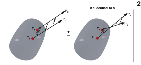
Figure 1: Schematic representation of the squared emission amplitude for two particles emitted independently from the grey-shaded source region and interacting with each other in the final states. For identical bosons (+) and fermions (-), correlation also involves interference between the paths.

Assumption 3: Smoothness approximation Anchishkin:1997tb ; Zhang:1997db ; Pratt:1997pw . Equation 6 is difficult to evaluate as it requires knowledge of the source function evaluated off-shell. For the special case where the particles do not interact aside from identical particle interference, $u_{q}(x_{a}-x_{b})=[e^{iq\cdot(x_{a}-x_{b})}\pm e^{iq\cdot(x_{b}-x_{a})}]/\sqrt{2}$, the integrals over $\tilde{q}$ and $\delta r^{\prime}$ can be performed analytically,

$$E_{a}E_{b}\frac{dN_{ab}}{d^{3}p_{a}d^{3}p_{b}} = \int d^{4}x_{a}d^{4}x_{b}\left\{s(p_{a},x_{a})s(p_{b},x_{b})\right.$$

$$\left.\pm s(P/2,x_{a})s(P/2,x_{b})\cos[(p_{a}-p_{b})\cdot(x_{a}-x_{b})]\right\}.$$

The source functions in the interference term are evaluated off-shell for non-zero $q$, $P_{0}/2\neq E({\bf P}/2)$. The smoothness approximation replaces $s(P/2,x_{a})s(P/2,x_{b})$ with either $s(E({\bf P}/2),{\bf P}/2,x_{a})s(E({\bf P}/2),{\bf P}/2,x_{b})$, which leads to Equation 3, or with $s(p_{a},x_{a})s(p_{b},x_{b})$, which leads to Equation 2. If the first approximation is performed, one should also make the same approximation for the denominator. The smoothness approximation has been checked for expanding thermal sources, where it was found to be very reasonable for large (RHIC-like) sources, but quite questionable for smaller sources such as those found in $pp$ or $e^{+}e^{-}$ collisions Pratt:1997pw .

Assumption 4: Equal time approximation. For the general case where the evolution operator incorporates Coulomb or strong interactions, deriving Equations 3 and 2 from Equation 6 is more complicated. First, the smoothness assumption amounts here to neglecting the $\tilde{q}$ dependence in the product of the source functions in Equation 6. This assumption is somewhat more stringent in the presence of final state interactions because the relevant range of $\tilde{q}$ extends beyond $q$. With this assumption, one obtains a $\delta$-function constraint for $\delta r^{\prime}$, and the integrand of (6) is proportional to the squared evolution matrix $|u_{q}^{\prime}(x_{a}^{\prime}-x_{b}^{\prime})|^{2}$. This evolution matrix has non-zero time components, which must be neglected if one is to identify it with the relative wave function. because the relative motion in the pair rest frame is small, one expects this approximation to be reasonable, but it has not yet been tested in model studies.

The above formalism is semi-classical in the sense that a quantum-mechanical particle emission probability, defined by the $T$-matrix elements, is usually approximated by classical source functions. As a consequence, quantum uncertainty limits the applicability of Equations 3 and 2. To illustrate this limitation, source functions have been evaluated by convoluting the emission function with wave packetsAichelin:1996iu ; Wiedemann:1997kq ; Wiedemann:1998ng ; Padula:1998ti of spatial width $\sigma$. This leads to a broadening of spatial distributions by $\left(\Delta R\right)^{2}\sim 0.5-1.0$ fm². because quantum smearing may already be incorporated into some of the semi-classical treatments through the choice of the initial density distribution, these calculations should be regarded as indicative of the theoretical uncertainty. because this error affects the size in quadrature, it is negligible for large sources, but might be significant for sources near 1 fm in size with strong space-time correlations Zhang:1997db ; Pratt:1997pw ; Wiedemann:1997kq ; Wiedemann:1998ng ; Martin:1998ku . In particular, analyses of $\pi\pi$ correlations from $e^{+}e^{-}$ collisions, which result in source sizes of less than 1.0 fmBarate:1999gj ; Abreu:1999xf , are difficult to interpret in the above formalism.

2.2 Identical-Particle Interference

In the absence of strong and electromagnetic final state interactions, the wave function of an identical particle pair in Equation 3 becomes

$$|\phi({\bf q}^{\prime},{\bf r}^{\prime})|^{2}-1=\pm\cos(2{\bf q}^{\prime}\cdot{\bf r}^{\prime}).$$ (8)

The distribution of separations in coordinate space ${\cal S}_{\bf P}({\bf r}^{\prime})$ can then be determined by performing a three-dimensional Fourier transform of $C({\bf q}^{\prime})-1$. It is instructive to consider the properties of this inversion in more detail. The curvature of $C({\bf q})$ at ${\bf q}=0$ can be related to the mean-square separation of the three-dimensional shape of ${\cal S}_{\bf P}({\bf r})$ (we neglect the ${\bf P}$ labels in $C$ and ${\cal S}$),

$$\left.\begin{array}[]{r}-\frac{d^{2}C({\bf q})}{dq_{i}^{\prime}\,dq_{j}^{\prime}}\end{array}\right|_{q=0}=\langle r_{i}r_{j}\rangle=\int d^{3}r{\cal S}({\bf r})r_{i}r_{j}.$$ (9)

This relation has been useful to qualitatively illustrate the relation between specific space-time information and specific features of the correlator. However, applying the identity quantitatively requires careful consideration of pions from longer-lived resonances which can dominate the calculation of $\langle r^{2}\rangle$ if not accounted for.

2.3 Correlations from Coulomb and Strong Interactions

Compared to the case for non-interacting identical particles, where the transformation between ${\cal S}_{\bf P}({\bf r})$ and $C({\bf P},{\bf q})$ is a Fourier transform, analyzing the experimentally measured correlation function with Equation 3 to determine the source function is more complicated. Understanding the resolving power of the kernel $|\phi({\bf q},{\bf r}|^{2}$ requires a detailed understanding of the relative wave function. Once one averages over spins, the squared relative wave function is a function of $q$, $r$ and $\cos\theta_{qr}$. In relativistic collisions, correlation analyses are usually confined to light, singly charged hadrons. Coulomb-induced correlations are then weak and must be analyzed at small $q$, where quantum effects become important ($qr/\hbar\sim 1$). The relative two-particle wave function in the presence of Coulomb interactions can then be written as a function of $qr/\hbar$, $r/a_{0}$ and $\cos\theta_{qr}$.

$$\phi = \Gamma(1+i\eta)e^{-\pi\eta/2}e^{i{\bf q}\cdot{\bf r}}\left\{1+\sum_{n=1}^{\infty}h_{n}\cdot(r/a_{0})^{n}\right\},$$ (10)

where $a_{0}$ is the Bohr radius, $h_{1}=1$ and $h_{n}=\frac{n-1-i\eta}{-in\eta}\,h_{n-1}$. Here, $\eta\equiv\mu e^{2}/\hbar q$ is independent of $r$, and for small $r/a_{0}$ the correlation function behaves as the Gamow factor, $G(\eta)\equiv e^{-\pi\eta}|\Gamma(1+i\eta)|^{2}=2\pi\eta/(e^{2\pi\eta}-1)$. Thus, the Coulomb kernels have little resolving power for $\pi\pi$ correlations where $a_{0}=387$ fm, but have greater resolving power for $pK$ correlations where $a_{0}=84$ fm.

For $r<<a_{0}$, the effects of Coulomb interactions can be removed easily from the correlation function because $\eta$ is independent of $r$ Gyulassy:1979yi ,

$$|\phi|^{2}\approx G(\eta)[1+\cos(2qr\cos\theta_{qr})]\,.$$ (11)

For realistic source sizes, the order $r/a_{0}$ corrections are of the order of 10% for $\pi\pi$ correlations and are larger for heavier pairs Anchishkin:1997tb ; Pratt:1986ev . Significant effort has been invested in “correcting” experimental correlation functions to remove Coulomb effects to all orders, but such corrections are model-dependent. The safest method for determining the source function is either inverting the full kernel Brown:2000aj ; Brown:1999ka ; Brown:1997ku ; Chung:2002vk ; Verde:2001md ; Verde:2003cx or fitting $C({\bf q})$ to some parameterized form for ${\cal S}({\bf r})$, which is convoluted with the full kernel. Neither of these tactics are computationally prohibitive.

Strong interactions can also be exploited to provide size and shape information. If the size of the source is much larger than the range of the potential between the two particles, the kernel $(|\phi|^{2}-1)$ can be determined entirely from knowledge of the phase shifts. Pairs that have a resonant interaction are especially useful, because the resonance will lead to a peak whose height is inversely proportional to the source volume, if $qR>>\hbar$. At small $q$ the kernel is determined by the scattering length, $a$ Wang:1999bf , and the height of the correlation at $q=0$ becomes

$$C({\bf q=0})-1=\left\langle-\frac{2a}{r}+\frac{a^{2}}{r^{2}}\right\rangle\,,$$ (12)

where the averaging is performed using ${\cal S}_{P}({\bf r})$ as a weight. Of course, the effects of strong interactions, Coulomb interference, and identical-particle interference can all combine as is the case for $pp$ correlations. The $pp$ kernel has been analyzed in depth by Brown and Danielewicz, where the kernel was inverted and applied to experimental $pp$ data. Evidence was seen for significant non-Gaussian behavior in the resulting source functions Verde:2001md ; Verde:2003cx . Strong interactions also provide angular resolving power Pratt:2003ar which can be understood from the perspective of classical trajectories. Even $s$-wave scattering can be exploited to discern information about shape.

Strong and Coulomb-induced correlations apply to both identical and non-identical particles. For non-identical particles, the wave function is not symmetrized and $|\phi({\bf q},{\bf r})|^{2}\neq|\phi({\bf q},-{\bf r})|^{2}$, which results in odd components of the correlations function, $C({\bf q})\neq C(-{\bf q})$ if there are odd components of ${\cal S}({\bf r})$ as is the case for non-identical particle pairs. This asymmetry can be experimentally exploited to investigate the spatio-temporal differences between the emission functions of different particle species Lednicky:1995vk ; Voloshin:1997jh ; this requires, however, sufficient statistics to select on the angle between the total and relative momentum in the pair center of mass $\angle({\bf q},{\bf P})$ Adams:2003qa .

2.4 Coordinate Systems

Correlation functions depend on two three-dimensional momenta, ${\bf P}$ and ${\bf q}$. For high-energy collisions, analyses are usually performed in the longitudinally comoving system (LCMS), a rest frame moving along the longitudinal (beam) direction such that $P_{z}=0$. Axes are usually chosen according to the out-side-long prescription. The longitudinal axis is chosen parallel to the beam, while the outward axis points in the direction of ${\bf P}$, which is perpendicular to the beam axis. The sideward axis is chosen perpendicular to the other two. If the system is boost-invariant, observables expressed in the LCMS variables are independent of $P_{z}$ and the source has a reflection symmetry about the $r_{\rm long}=0$ plane. If the collision is central, there is also a reflection symmetry about the $r_{\rm side}=0$ plane. Any four-vector $V$ can be expressed in this coordinate system using the four-momentum $P$ to project out the componentsPratt:1986cc ; Bertsch:1989vn ; Csorgo:1989kq ,

$$V_{\rm long} = (P_{0}V_{z}-P_{z}V_{0})/M_{T},$$ (13)

$$V_{\rm out} = (P_{x}V_{x}+P_{y}V_{y})/P_{T},$$

$$V_{\rm side} = (P_{x}V_{y}-P_{y}V_{x})/P_{T},$$

where $M_{T}^{2}=P_{0}^{2}-P_{z}^{2}$ and $P_{T}^{2}=P_{x}^{2}+P_{y}^{2}$. Dimensions of the source function are typically quoted in this coordinate system. One could also perform a second boost to the pair frame, in which the transverse components of the total momentum are zero. Then,

$$V_{\rm out}^{\prime}=\frac{M_{\rm inv}}{M_{T}}\frac{(P_{x}V_{x}+P_{y}V_{y})}{P_{T}}-\frac{P_{T}}{M_{T}M_{\rm inv}}P\cdot V,$$ (14)

where $M_{\rm inv}^{2}=P^{2}$. Relative wave functions are more conveniently expressed in the frame of the pair. For instance, a sharp resonant peak is no longer sharp if the correlation is viewed away from the pair frame. For pairs where the correlation is influenced by Coulomb and strong interactions, most analyses are conducted in the pair frame.

For non-zero impact parameters, azimuthal symmetry is lost and source functions also depend on the azimuthal direction of the pair’s total momentum Wiedemann:1997cr ; Lisa:2000ip ; Heinz:2002au . Also, if boost-invariance is broken, the pair’s rapidity needs to be specified. In this more general case, reflection symmetries are broken and the choice of the coordinate axes becomes somewhat arbitrary. One could orient the axes according the event’s impact parameter, or one could rotate the coordinate system so that in the new frame cross terms such as $\langle xy\rangle$ vanish (illustrated in Figure 2). One would then specify the Euler angles as part of the description of the source function.

2.5 Gaussian Parameterizations

To gain a physical understanding of the three-dimensional spatio-temporal source distribution, it is useful to summarize its size and shape with a few parameters. This motivates the study of Gaussian parameterizations for the source ${\cal S}_{\bf P}({\bf r}^{\prime})$ and the two-particle correlator. Realistic sources deviate from Gaussians, e.g. by exponential tails caused by resonance decay contributions. The extracted Gaussian source parameters may thus depend on details of the fitting procedures. These shortcomings can be overcome with imaging methods, or more complicated forms for the fitting. A more general three-dimensional analysis of correlations would involve decomposing both the correlation and source functions in either spherical or Cartesian harmonics Danielewicz:2005qh ; ZibiMikeTom . Although the detailed non-Gaussian aspects of the correlation are important, the extra information can also cloud the main trends in the data. In practice, Gaussian parameterizations provide the standard minimal description of experimental data.

2.5.1 The general case

The most general form for a Gaussian source is $\exp\{-A_{\alpha\beta}(x_{\alpha}-\bar{x}_{\alpha})(x_{\beta}-\bar{x}_{\beta})\}$, where $x_{\alpha}$ refers to the four dimensions $x,y,z,t$, and $A$ is a $4\times 4$ real symmetric matrix. The most general form has 14 parameters, 10 parameters for $A$ and four more parameters for the offsets $\bar{x}_{\alpha}$. Reflection symmetries can be used to eliminate certain cross terms and some of the offsets Chapman:1995nz . Furthermore, if the particles are identical or have the same phase space distributions, all the offsets can be set to zero. because the source function for the second species $b$ might also have 14 parameters, there could be up to 28 Gaussian parameters in describing both $s_{a}$ and $s_{b}$. However, because ${\cal S}({\bf r})$ depends only on the distribution of relative spatial coordinates in the pair frame, only nine Gaussian parameters are required to describe the most general ${\cal S}$ for a given ${\bf P}$. Three of these nine parameters can be identified with Gaussian widths, three can be identified with offsets, and the last three can either be identified with cross terms or with the three Euler angles describing the orientation of the three-dimensional ellipse.

Using the reflection symmetries for mid-rapidity sources in a symmetric central collision, a Gaussian parameterization of the emission function for particle species $a$ in the out-side-long coordinate system reads

$$s_{a}(p,x) \sim \exp\left\{-\frac{(x_{\rm out}-\bar{x}_{a,{\rm out}}-V_{s,a}(t-\bar{t}_{a}))^{2}}{2R_{a,{\rm out}}^{2}}\right.$$

$$\hskip 48.0pt\left.-\frac{(x_{\rm side})^{2}}{2R_{a,{\rm side}}^{2}}-\frac{(x_{\rm long})^{2}}{2R_{a,{\rm long}}^{2}}-\frac{(t-\bar{t}_{a})^{2}}{2(\Delta\tau_{a})^{2}}\right\}.$$

The symmetries forbid any cross terms in the exponential involving $x_{\rm side}$ or $x_{\rm long}$, such as $x_{\rm side}x_{\rm out}$ or $x_{\rm long}t$, but do not forbid a cross term between outward position $x_{\rm out}$ and time $t$. Here, this cross term is taken into account by allowing the source to move in the outward direction with a velocity $V_{s}$. The symmetries also forbid offsets in the sideward or longitudinal direction. These other offsets have also been addressed for non-central collisions Retiere:2003kf ; Miskowiec:1998ms .

The correlation function is determined by the phase space density of the final state, Equation 27. The resulting phase space density is

$$f_{a}({\bf p},{\bf r},t) \sim \exp\left\{-\frac{\left[x_{\rm out}-\bar{X}_{a}(t)\right]^{2}}{2\left[R_{a,{\rm out}}^{2}+(V_{s,a}-V_{\perp})^{2}(\Delta\tau_{a})^{2}\right]}-\frac{x_{\rm side}^{2}}{2R_{a,{\rm side}^{2}}}-\frac{x_{\rm long}^{2}}{2R_{a,{\rm long}^{2}}}\right\},$$

$$\bar{X}_{a}(t) = \bar{x}_{a,{\rm out}}+V_{\perp}(t-\bar{t}_{a}).$$ (16)

Here, $V_{\perp}$ is the velocity of the pair in the LCMS frame.

The correlation function is determined by the relative distance function ${\cal S}_{\bf P}({\bf r}^{\prime})$, see Equation 3,

$${\cal S}_{\bf P}({\bf r}^{\prime}) \sim \exp\left\{-\frac{\left[r^{\prime}_{\rm out}-\bar{X}_{\rm out}\right]^{2}}{4\gamma_{\perp}^{2}R_{\rm out}^{2}}-\frac{r_{\rm side}^{\prime 2}}{4R_{\rm side}^{2}}-\frac{r_{\rm long}^{\prime 2}}{4R_{\rm long}^{2}}\right\}$$ (17)

$$R_{\rm out}^{2} = \frac{1}{2}\left[R_{a,{\rm out}}^{2}+R_{b,{\rm out}}^{2}+(V_{s,a}-V_{\perp})^{2}(\Delta\tau_{a})^{2}+(V_{s,b}-V_{\perp})^{2}(\Delta\tau_{b})^{2}\right],$$

$$R_{\rm side}^{2} = \frac{1}{2}\left[R_{a,{\rm side}}^{2}+R_{b,{\rm side}}^{2}\right],~{}~{}~{}R_{\rm long}^{2}=\frac{1}{2}\left[R_{a,{\rm long}}^{2}+R_{b,{\rm long}}^{2}\right],$$

$$\bar{X}_{\rm out} = \bar{x}^{\prime}_{a,{\rm out}}-\bar{x}^{\prime}_{b,{\rm out}},$$

where $\gamma_{\perp}\equiv(1-V_{\perp})^{-1/2}$. Thus, there are four measurable parameters, $R_{\rm out}$, $R_{\rm side}$, $R_{\rm long}$, and $\bar{X}_{\rm out}$. In the absence of any symmetry, there are five more terms: three cross terms $(R^{2}_{\rm out,side},R^{2}_{\rm out,long}$ and $R^{2}_{\rm side,long})$, and two more offsets ($X_{\rm side}$ and $X_{\rm long}$). For identical particles, all the offsets are zero.

2.5.2 Sensitivity to Lifetime

Given the symmetries used to derive Equation 17, the most experiment can provide is the determination of the four parameters, $R_{\rm out}$, $R_{\rm side}$, $R_{\rm long}$, and $\bar{X}_{\rm out}$. The only way to independently determine the lifetime is to assume that the two transverse spatial sizes are approximately equal Heinz:1996qu . After assuming $R_{a,{\rm out}}^{2}+R_{b,{\rm out}}^{2}\approx R_{b,{\rm side}}^{2}+R_{b,{\rm side}}^{2}$, Equation 17 yields for identical particles ($V_{a,s}=V_{b,s}=V_{s},\Delta\tau_{a}=\Delta\tau_{b}=\Delta\tau$),

$$(V_{\perp}-V_{s})^{2}(\Delta\tau)^{2}\approx R_{\rm out}^{2}-R_{\rm side}^{2}\ .$$ (18)

In general, however, the source velocity is not precisely known and outward and sideward spatial dimensions are not exactly equal; these factors result in a significant systematic error when applying Equation 18, especially because temporal effects enter in quadrature. The $R_{\rm out}/R_{\rm side}$ ratio only provides a reliable estimate of the lifetime when $(V_{\perp}-V_{s})\Delta\tau$ is much larger than the transverse size.

2.5.3 Gaussian Cross Terms

In addition to the three Gaussian parameters, $R_{\rm out}$, $R_{\rm side}$ and $R_{\rm long}$, that describe the dimensions of a Gaussian source, one needs, in the general non-symmetric case, three more parameters to describe the angular orientation of the principal axes. Figure 2 displays how the principal axes might differ from the out-side-long axes once the collisions are off center. These three Euler angles combined with three sizes can also be related to the parameters $A_{ij}$ in the general form for a three-dimensional Gaussian, $\exp(-A_{ij}r_{i}r_{j})$, where $A$ is a symmetric matrix with six independent components Voloshin:1995mc ; Chapman:1995nz ; Wiedemann:1997cr ; Heinz:2002au .

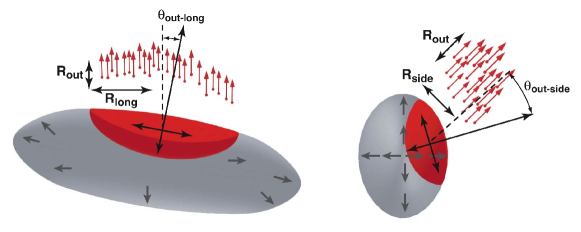
Figure 2: For non-central collisions the principal axes describing the orientation of the region of homogeneity can differ from the out-side-long axes. By viewing the source distribution from the perspective where the beam axis is oriented horizontally (left panel) and from peering down the beam pipe (right panel), the orientations leading to out-long and out-side cross terms are illustrated.

For pairs of identical particles, the correlation function for Gaussian sources is also Gaussian,

$$C({\bf q})=1+\exp(-({\cal R}^{2})_{ij}Q_{i}Q_{j})\,,$$ (19)

where $Q=2q$. The six experimentally determined parameters, $({\cal R})^{2}_{ij}$, can be related to the moments of ${\cal S}({\bf r}^{\prime})$ Wiedemann:1996ej ,

$$\langle r_{i}r_{j}\rangle=({\cal R}^{2})_{ij}.$$ (20)

For central collisions, the source sizes $(R^{2})_{ij}$ depend only on the longitudinal pair momentum $P_{L}$ and on the modulus of the transverse pair momentum $|\vec{P}_{T}|$. This is different for non-central collisions for which the azimuthal direction $\phi_{\rm pair}=\angle(\vec{P}_{T},\hat{b})$ of the transverse pair momentum with respect to the impact parameter direction $\hat{b}$ matters. The $\phi_{\rm pair}$-dependences of $(R^{2})_{\rm out}$, $(R^{2})_{\rm side}$, and $(R^{2})_{\rm out-side}$ then characterize the degree to which the initially out-of-plane-extended source geometry has expanded to the point where it becomes in-plane-extended Wiedemann:1997cr ; Lisa:2000ip . The out-longitudinal and side-longitudinal cross terms contain information about the extent to which the main axis of the emission ellipsoid is tilted with respect to the beam axisLisa:2000ip . We return to this topic in Section 4.2.

The Yano-Koonin parameterization Yano:1978gk ; Wu:1996wk ; Chapman:1995nz ; Chapman:1994yv provides an alternative basis for describing the out-long cross term. The Yano-Koonin form is based on the assumption that one can boost along the beam axis to a source frame where the correlation function has a simple form.

$$C({\bf P},{\bf Q})=1+\exp\left\{-\tilde{Q}_{\perp}^{2}R_{\perp}^{2}-\tilde{Q}_{||}^{2}R_{||}^{2}-\tilde{Q}_{0}^{2}R_{0}^{2}\right\}\ ,$$ (21)

where ${\tilde{Q}}$ is the momentum difference defined in the source frame which has rapidity $y_{\rm YK}$. In that frame $R_{0}$ is the Gaussian lifetime and $R_{\perp}$ and $R_{||}$ are the dimensions of the source. This can be transposed to the out-long-side frame by boosting $\tilde{Q}$ along the beam axis to the frame where $P_{z}=0$, i.e. the LCMS frame, then using the fact that $Q_{0}=Q_{\rm out}P_{\perp}/P_{0}\equiv Q_{\rm out}V_{\perp}$ in the new frame. This yields $\tilde{Q}_{0}=\cosh(y_{\pi\pi}-y_{YK})Q_{\rm out}V_{\perp}-\sinh(y_{\pi\pi}-y_{\rm YK})Q_{\rm long}$, and $\tilde{Q}_{||}=\cosh(y_{\pi\pi}-y_{YK})Q_{\rm long}-\sinh(y_{\pi\pi}-y_{\rm YK})Q_{\rm out}V_{\perp}$, where $y_{\pi\pi}$ is the rapidity of the LCMS frame. Substituting these expressions into Equation 21 yields a cross term in the exponential equal to $Q_{\rm out}Q_{\rm long}(R_{0}^{2}+R_{||}^{2})\sinh 2(y_{\pi\pi}-y_{\rm YK})$, which disappears when $y_{YK}=y_{\pi\pi}$. By fitting $y_{YK}$ as a function of the pair rapidity, aspects of boost invariance can be tested. Given that the distribution of source rapidities should fall off for large rapidities, one expects $y_{YK}$ to lag $y_{\pi\pi}$, because pions of a given rapidity would more likely have been emitted from sources with smaller rapidities Wu:1996wk .

2.6 The $\lambda$ factor

Many pions measured in experiment come from long-lived decays. Pions from weak decays may or may not, depending on the experiment, be identified and removed from the analysis, because their decay vertices are typically a few centimeters from the reaction center. Decays from $\eta$ or $\eta^{\prime}$ mesons occur a few thousand fm away from the center of the collision. At these distances, they are effectively uncorrelated with other particles but cannot be identified with experiment. If a fraction $\lambda$ of the pairs originate from the spatio-temporal region relevant for correlations, the correlation is muted by the factor $\lambda$ Gyulassy:1979yi . If the source function is divided into two contributions, ${\cal S}({\bf r})=\lambda{\cal S}_{\rm local}+(1-\lambda){\cal S}_{\infty}$, where both ${\cal S}_{\rm local}$ and ${\cal S}_{\infty}$ integrate to unity, the resulting correlation is

$$C({\bf q})=(1-\lambda)+\lambda\int d^{3}r^{\prime}{\cal S}_{\rm local}({\bf r}^{\prime})\left[|\phi({\bf q}^{\prime},{\bf r}^{\prime})|^{2}-1\right].\\$$ (22)

If the experimental sample includes a contamination from weak decays, $\eta$, or mis-identified particles of a fraction $f$, the lambda factor becomes $(1-f)^{2}$. It is not uncommon for this contamination factor to be near 30%, which results in $\lambda$ near one half.

Certainly, this division is somewhat artificial, as there are non-Gaussian tails, or halos Csorgo:1994in , to ${\cal S}_{\rm local}$ due to such causes as the exponential fall-off of the source function in the longitudinal direction or semi-long-lived resonances such as the $\phi$, whose lifetime is 40 fm/c. Non-Gaussian behavior is a subject for either imaging Brown:2000aj ; Brown:1999ka ; Brown:1997ku ; Chung:2002vk ; Verde:2001md ; Verde:2003cx or for more complicated parameterizations.

The $\lambda$ factor is often referred to as an incoherence factor, the name being motivated by the properties of a coherent state, $\exp\{i\int d{\bf p}\eta({\bf p})[a({\bf p})+a^{\dagger}({\bf p})]\}|0\rangle$, which for identical particles leads to no correlation. Coherent states represent highly correlated emissions caused by phase coherence and thus violate the assumption of incoherence or uncorrelated emission implied by Assumption 2 as described early in this section. The question of whether an observation of $\lambda\neq 1$ is due to coherence or due to contamination from particles from far outside the source volume can be tested by analyzing three-particle correlations Heinz:1997mr ; Heinz:2004pv . Such analyses of data at both SPS and RHIC have been consistent with the incoherence conjecture Boggild:1999tu ; Bearden:2001ea ; Adams:2003vd . Microscopic model calculations at the AGS reproduce the excitation function of $\lambda$ when resonances contributions are included Lisa:2000no .

2.7 Collective Flow and Blast-Wave Models

Both longitudinal and radial collective expansion reduce the size of the region of homogeneity, i.e., the relevant volume for particles of a given velocity. For an infinite volume, the size of this region is set by the length one must move before collective velocity overcomes the thermal velocity, $R\sim V_{\rm therm}/(dv/dz)$.

2.7.1 Longitudinal Flow

The Gaussian lifetime $\Delta\tau$ described in Equation 18 represents the spread of the emission times. A small value of $\Delta\tau$ does not imply that particles were emitted early, but that they were emitted suddenly. Inferring the mean time at which particles are emitted requires a different assumption. For instance, at RHIC, the initial nuclei are Lorentz contracted by a factor of 100, and if there were no subsequent expansion, $R_{\rm long}$ would be less than a Fermi. If one assumes that the system expands along the beam axis with no longitudinal acceleration, the collective velocity becomes

$$V_{{\rm coll},z}=z/t.$$ (23)

If emission then comes from sources moving over a large range of rapidities (a boost-invariant expansion), the dimension along the beam axis for the source emitting zero-rapidity particles is determined by the distance one can move before the collective velocity overwhelms the thermal velocity to force the emission function back to zero. The size can then be expressed as:

$$R_{\rm long}\approx\frac{V_{\rm therm}}{dv/dz}=V_{\rm therm}\langle t\rangle.$$ (24)

Whereas $R_{\rm out}/R_{\rm side}$ gives information about the suddenness of emission, $R_{\rm long}$ provides insight into the mean time at which emission occurs given an estimate of the thermal velocity.

For a thermal source with relativistic motion, the thermal velocity along the beam axis is determined by the temperature and the transverse mass, $m_{T}=\sqrt{m^{2}+p_{T}^{2}}$ Pratt:1986cc . For large $m_{T}$ the thermal velocity in the longitudinal direction becomes non-relativistic, $V_{\rm therm}=\sqrt{T/m_{T}}$, and the source size falls as $1/\sqrt{m_{T}}$ which is referred to as $m_{T}$ scaling Makhlin:1987gm . This is illustrated in Figure 3. However, this assumes all particles are emitted with the same Bjorken time $\tau_{B}$ and temperature, independent of the transverse mass. because particles with high $m_{T}$ are probably emitted at lower $\tau_{B}$, and because the temperature roughly behaves at $\tau_{B}^{-4/3}$, the longitudinal size could fall even more quickly than $m_{T}^{-1/2}$.

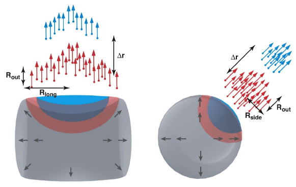
Figure 3: because particles with heavier masses have smaller thermal velocities, their source volumes are more strongly confined by collective flow. For longitudinal flow (left panel) this results in smaller values of $R_{\rm long}$ for particles with higher $m_{T}=\sqrt{m^{2}+p_{T}^{2}}$. For radial flow (right panel) this confines heavier particles toward the surface, which results in both a reduced volume and an offset $\Delta r$ in the outward direction.

In a boost invariant expansion, emission is a function of the Bjorken time $\tau_{B}=\sqrt{t^{2}-z^{2}}$, not the time $t$, and because $t=\sqrt{\tau_{B}^{2}+z^{2}}$, those particles emitted with small $z$ have a head start. This is sometimes referred to as an inside-outside cascade. The transverse shape of ${\cal S}({\bf r})$ is then affected non-trivially by the expansion along the beam. The resulting correlation function can be calculated analytically in the case of pure identical-particle correlations Kolehmainen:1986fe ; Padula:1989ie .

Boost invariance is incorporated into blast-wave models with transverse expansion and assumed for many hydrodynamic models. The finite size of the system would alter the results for two reasons. First, if the distribution of sources covers only a finite range in $\eta$, the tails of the distribution ${\cal S}({\bf r})$ are chopped off. Assuming the distribution in $\eta$ is Gaussian rather than uniform,

$$\frac{1}{R_{\rm long}^{2}}\sim\frac{1}{V_{\rm therm}^{2}\tau_{B}^{2}}+\frac{1}{\eta_{G}^{2}\tau_{B}^{2}},$$ (25)

where $\eta_{G}$ is the range of rapidities over which the sources are distributed. If $\eta_{G}$ were 1.5 units of rapidity, the extracted values of $\tau_{B}$ from boost-invariant pictures would be underestimating $\tau_{B}$ by $\sim 10$%.

A second shortcoming of boost-invariant models is that they ignore acceleration in the longitudinal direction. Accounting for this acceleration would alter the relation between the time and the velocity gradient. Neglecting this acceleration could also lead to a modest underestimate of $\tau_{B}$ Renk:2003gn .

2.7.2 Transverse Collective Flow

because transverse collective flow is intimately related to the pressure and viscosity, it is of central importance. Blast-wave models are based on pictures of thermal sources superimposed onto the transverse and longitudinal collective velocity profiles. Simple forms are then chosen for the profiles. Only two parameters are important for analyzing spectra, the temperature and the transverse velocity. because heavier particles are more sensitive to flow than are light particles, the two parameters can be adjusted to fit the spectra of several species.

In addition to the temperature and transverse velocity, correlation measurements are also sensitive to the space-time parameters of the blast wave. In a minimal parameterization this would include the lifetime $\tau_{B}$ and the transverse size $R$. More sophisticated models would also include a spread in lifetime $\Delta\tau$ and a surface diffuseness $\Delta R$. Additional parameters ensue when one considers sensitivity to the reaction plane. Then, two parameters are needed to describe the transverse size, and two parameters are required to describe the transverse collective velocity. These parameters can then depend on the azimuthal direction of ${\bf P}$ Heinz:2002sq .

Choosing a blast-wave parameterization involves a number of choices about the form of the parameterization Tomasik:2001uz . Chemical potentials and temperatures might be chosen to vary with the transverse position $r$ Chojnacki:2004ec ; Csorgo:2001xm or might be chosen to be uniform. A wide variety of parameterizations have been employed for the transverse velocity profile, which might choose linear profiles for either $v$, $\gamma v$ or the transverse rapidity $asinh(\gamma v)$. In some parameterizations, the velocity profile has been chosen to rise quadratically with $r$ Lee:1990sk ; Schnedermann:1993ws . Although hydrodynamics has been invoked as justification for different parameterizations, profiles from hydrodynamics vary according to the equation of state.

For particles moving much faster than the surface velocity, transverse flow manifests itself by constraining particles to an increasingly small fraction of the blast-wave volume for the same reason that $R_{\rm long}$ falls with $m_{T}$ owing to longitudinal expansion Pratt:1984su . For large $m_{T}$, this leads to both $R_{\rm side}$ and $R_{\rm out}$ falling as $1/\sqrt{m_{T}}$ Chapman:1995nz ; Chojnacki:2004ec ; Csorgo:2001xm ; Sinyukov:1998ex . The fact that transverse dimensions fall with $m_{T}$ might also result from the dynamics of cooling, superimposed with a growing fireball. This correlates high-energy particles with earlier times when the fireball was both smaller and at a higher temperature.

Non-identical particles are of special interest in a blast-wave. For particles moving faster than the surface of the blast wave, there is a stronger tendency for heavier particles to be more confined to the region of the surface owing to their slower thermal velocities Retiere:2003kf . This results in heavy particles being ahead of lighter particles of the same asymptotic velocity, and leads to a non-zero $\Delta{\bf r}$ illustrated in Figure 3. As discussed in Section 2.3, these displacements are accessible through measuring odd components of the correlation function Lednicky:1995vk ; Voloshin:1997jh ; Adams:2003qa .

2.8 Generating Correlations Functions from Hydrodynamics and from Microscopic Simulations

Any model that predicts final-state space-time and momentum information of emitted particles can be used to predict correlation functions. This information may be extracted from both microscopic simulations or from hydrodynamic calculations.

Microscopic simulations model the collision by evolving particles along straight-line classical trajectories which are punctuated by collisions that are programmed to be consistent with free-space cross-sections. When the modeling is done on a one-to-one basis, the simulations are referred to as cascades. Boltzmann simulations are similar but employ an oversampling by a factor $N_{s}$ accompanied by a scaling down of the cross-sections by the same factor. These are then consistent with the Boltzmann equation and become local and relativistically covariant in the large $N_{s}$ limit Molnar:2000jh ; Cheng:2001dz . To generate correlation functions from either class of simulation, there are essentially two methods which are equally justified within the smoothness approximation. Method I is motivated by Equation 3. This involves first creating two lists, one for each species, of the space time coordinates $x_{a}$ and $x_{b}$ of all those particles that were emitted with momenta $m_{a}{\bf P}/(m_{a}+m_{b})$ and $m_{b}{\bf P}/(m_{a}+m_{b})$. From these lists, one generates ${\cal S}_{\bf P}({\bf r})$ by sampling the distributions of $x_{a}-x_{b}$. This list is then convoluted with $|\phi({\bf q},{\bf r})|^{2}$ to generate $C({\bf P},{\bf q})$ for all ${\bf q}$. In Method II, one samples pairs randomly without regard to their momenta. The numerator of the correlation function is then calculated by generating pairs with the same weight as one expects to observe experimentally and applying a weight given by the square of the relative wave function. The denominator would be calculated in a similar manner, but without the weight from the wave function. This method reflects the description of the correlation function in Equation 2. Acceptance effects or kinematic cuts can then be performed exactly as they would be performed for real particles. Method II has an advantage in that it is easier to accurately incorporate acceptance effects or tight kinematic cuts. Method I makes for a much quicker calculation because the procedure does not require sampling particles for irrelevant momenta Zhang:1997db .

Given the equation of state and the initial energy density, hydrodynamics provides the means for solving for the space-time development of the stress-energy tensor which can be used to make predictions for correlations Kolb:2003dz ; Huovinen:2001cy ; Hirano:2004ta . Viscous effects can also be incorporated and are non-negligible Heinz:2001xi ; Teaney:2003pb . Generating source functions from the output of hydrodynamic calculations is not as straightforward as it might seem. The Cooper-Frye prescription Cooper:1974qi conserves energy and momentum if the equation of state is one of free particles, but it suffers from the fact that the particles that cross backwards across the surface into the hydrodynamic volume enter the source function as a negative emission probability. If the relative velocity of the surface, as measured by an observer in the matter’s rest frame, is not much faster than the thermal velocity, a different prescription is required. Numerous prescriptions have been proposed to address these issues Tomasik:2002qt ; Csernai:2004pr ; Sinyukov:2002if .

Hydrodynamic models, even those that incorporate viscosity, cannot be justified once the system expands to the point that the mean free path is similar to the characteristic size of the system. However, Boltzmann descriptions or cascades are well justified at lower densities. Several efforts have thus focused on coupling the two approaches Soff:2000eh ; Bass:2000ib ; Teaney:2001gc ; Teaney:2001av . because the final-state trajectories are established in the Boltzmann part of the prescription, one can apply either of the methods mentioned above.

2.9 Phase Space Density, Entropy and Coalescence

because phase space density depends on both the momentum ${\bf p}$ and the position ${\bf r}$, a measurement of the phase space density must specify the spatial region over which it is determined. In practice, spatial information from two-particle correlation functions is instrumental to this end. For identical particle pairs, the “area” under the correlation function determines the average phase space density Bertsch:1994qc . Substituting the final phase space density for the time-integrated source function,

$$\int^{t_{f}}\frac{dx_{0}}{E_{p}(2\pi)^{3}}s(p,x)|_{p_{0}=E_{p}}=f({\bf p},{\bf x},t_{f})\,,$$ (26)

and inserting into Equation 3 with $Q=2q$ leads to

$$\int d^{3}Q\left[C({\bf Q})-1\right] = (2\pi)^{3}\frac{\int d^{3}r|f({\bf P}/2,{\bf r},t_{f})|^{2}}{\left[\int d^{3}rf({\bf P}/2,{\bf r},t_{f})\right]^{2}}=\frac{\bar{f}({\bf P}/2)}{dN/d^{3}p}\,,$$ (27)

$$\bar{f}({\bf p}) = \frac{(2\pi)^{3}}{(2S+1)}\frac{E_{p}}{m}\frac{dN}{d^{3}p}{\cal S}_{{\bf P}=2{\bf p}}({\bf r}^{\prime}=0).$$

Equation 2.9 applies also for the case of non-identical particles of the same phase space density. We note that $\bar{f}({\bf p})$ is the phase space density averaged over coordinate space for a specific momentum using the phase space density itself as the weight. Unless $f({\bf p},{\bf r},t)$ is a constant within a fixed volume, the average phase space density will fall below the maximum phase space density Tomasik:2002qt . For instance, if $f({\bf p},{\bf r},t)$ has a Gaussian profile in coordinate space, the average phase space density will be $2^{-3/2}$ of the maximum phase space density for that momentum. For a Gaussian source,

$$\bar{f}({\bf p})=\frac{\pi^{3/2}}{(2S+1)mR_{\rm inv}^{3}}E\frac{dN}{d^{3}p},$$ (28)

where $R_{\rm inv}^{3}=(E/m)R_{\rm out}R_{\rm side}R_{\rm long}$ is the product of the three radii as measured in the frame of the pair. The phase space density is determined by combining a source size measurement with the spectra. Entropy can be related to the phase space density in the standard way Pal:2003rz

$$S = (2S+1)\int\frac{d^{3}rd^{3}p}{(2\pi)^{3}}\left[-f\ln f\pm(1\pm f)\ln(1\pm f)\right],$$ (29)

$$dS/dy \approx \int d^{2}p_{T}~{}E\frac{dN}{d^{3}p}\left[\frac{5}{2}-\ln(2^{3/2}\bar{f}({\bf p}))\pm\bar{f}({\bf p})/2\right]\,.$$ (30)

Here, Equation 30 ignores higher powers of $\bar{f}$.

The average phase space density is also straightforward to determine by constructing ratios of spectra with species that can either bind or form a resonance. If species $a$ and $b$ can bind to form species $c$, thermal arguments would state

$$f_{c}({\bf r},t)=f_{a}({\bf P}m_{a}/m_{c},{\bf r},t)f_{b}({\bf P}m_{b}/m_{c},{\bf r},t)e^{B/T},$$ (31)

where $B$ is the binding energy, or the excitation energy if the resonance is unstable. Coalescence arguments, which give the same expression but without the binding energy Danielewicz:1991dh ; LlopeCoalescence , are identical if the binding energy is small compared to the temperature, as is the case for nucleon coalescence. The average phase space density for $a$ or $b$ can be determined by inserting Equation 31 into Equation 2.9,

$$\bar{f}_{a,b}({\bf p})=e^{-B/T}\frac{m_{b,a}(2S_{b,a}+1)}{m_{c}(2S_{c}+1)}\frac{E_{c}dN_{c}/d^{3}P}{E_{b,a}dN_{b,a}/d^{3}p}.$$ (32)

Here, the binding energy needs to be expressed in the frame of the thermal bath. For the case where $B$ is small, the assumption of a thermal bath can be neglected. Two examples where particles with similar phase-space densities form low-energy resonances or bound states are $pn\rightarrow d$ and $\phi\rightarrow K^{+}K^{-}$.

By comparing the expression for $\bar{f}$ from the ratio of spectra in Equation 32, with Equations 2.9 or 28, one can determine either ${\cal S}_{\bf P}({\bf r}^{\prime}=0)$ or the Gaussian parameters from ratios of spectra.

$${\cal S}_{\bf P}({\bf r}^{\prime}=0) = e^{-B/T}\frac{m_{a}m_{b}(2S_{a}+1)(2S_{b}+1)}{(2\pi)^{3}m_{c}(2S_{c}+1)}\frac{E_{c}dN_{c}/d^{3}P}{E_{a}dN_{a}/d^{3}p_{a}\cdot dN/d^{3}p_{b}},$$ (33)

$$R_{\rm inv}^{3}({\bf P}) = \frac{1}{(4\pi)^{3/2}{\cal S}_{\bf P}({\bf r}^{\prime}=0)}.$$ (34)

Coalescence analyses can provide powerful measurements of volumes, but they only provide a single number, ${\cal S}({\bf r}^{\prime}=0)$, and they cannot provide any insight into either the shape or the $r$ dependence.

3 Femtoscopic measurements

Experimental techniques have developed considerably in response to significant improvements in both the theory and the quantity and quality of experimental data. In this section we discuss the general experimental approach for defining and analyzing femtoscopic correlations and their systematic dependence on global and kinematic quantities.

3.1 Correlation Function Definition

In practice, the formal definition of the correlation function in Equation 1 is seldom used in heavy ion physics. Instead the correlation of two particles, $a$ and $b$ for a given pair momentum ${\bf P}$ and relative momentum ${\bf q}$, is nominally given by

$$C^{ab}_{\bf P}({\bf q})=\frac{A^{ab}_{\bf P}({\bf q})}{B^{ab}_{\bf P}({\bf q})}\cdot\xi_{\bf P}({\bf q}),$$ (35)

where ${A^{ab}_{\bf P}({\bf q})}$ is the signal distribution, ${B^{ab}_{\bf P}({\bf q})}$ is the reference or background distribution which is ideally similar to $A$ in all respects except for the presence of femtoscopic correlations, and $\xi_{\bf P}({\bf q})$ is a correction factor introduced to compensate for non-femtoscopic correlations present in the signal that are not fully accounted for in the background as well as artifacts resulting, e.g., from finite resolution and contamination.

3.2 Signal Construction

The signal ${A^{ab}_{\bf P}({\bf q})}$ refers to the relative momentum distribution of particles $a$ and $b$ for a given range of pair momenta, ${\bf P}$, and a given set of event characterizations. Although not all analyses proceed in exactly the following fashion, the mechanics of constructing the signal and background are most easily understood if one considers as separate steps:

1. Event quality cuts and event-class binning;

2. Single-track (including particle identification) cuts and single-particle binning; and

3. two-particle pairing, two-track cuts, and pair momenta binning.

Here the term event class refers to both physics observables, such as collision centrality and reaction plane orientation, and detector considerations, such as event vertex position and the condition of the detector when the event was recorded, usually keyed by run number. The latter considerations are relevant to the proper construction of the background. For event-class, particle, and pair bin, the final signal is usually stored as a set of 3D-histograms in the canonical relative momentum variables.

Single-particle acceptances divide out with a properly constructed background, but 2-track acceptances can have a large effect on the correlation function. For this reason the analysis of 2-track cuts is the dominant consideration in the signal construction for most analyses. The cuts and terminology are different for Time Projection Chamber (TPC) experiments with near continuous hit distributions and Drift Chamber experiments with projective geometry, but the goals are the same. Split-tracks Adams:2004yc ; Lisa:2005vw and ghost-tracks both refer to single tracks which are incorrectly reconstructed as a pair of tracks with very low relative momenta. Even after the event-reconstruction algorithms (which generate a list of individual tracks) have been optimally tuned, small traces of these false pairs remain and must be removed from the analysis with identical pairwise cuts. Usually only a tiny fraction of tracks are split, and this effect may be ignored in essentially all experimental analyses except femtoscopic ones. Various methods have been developed for identifying likely split tracks, usually based on the number Lisa:2005vw or topology Adams:2004yc of space-points associated with the track.

Pairwise effects usually also result in the loss of pairs at low relative momentum, because two tracks with very similar trajectories tend to be reconstructed as a single track. (Note that in tracking detectors, this is not a problem if one or both of the particles is a topologically identified neutral particle. In that case, the decay daughters may be well-separated even if their parents have identical momentum.) Such merging issues are usually resolved by pairwise cuts that remove merged pairs. Developing efficient and appropriate cuts can be a subtle exercise, and it requires good knowledge of the detector and event reconstruction software. In most cases these cuts are supported by simulations, but final determinations are nearly always based upon data.

What does it mean to cut out merged pairs? After all, if the tracks have merged, then the pair is lost anyway. The point is twofold. First, the pair efficiency usually does not drop from 100% to 0% sharply as a function of any variable. Thus, the cuts are usually tuned to exclude all Lisa:2000no ; Adams:2004yc or most Boggild:1994vk ; Ahle:2002mi ; Adler:2004rq of the inefficient region. If regions with less than perfect efficiency remain in the analysis, a 2-track efficiency correction based on Monte Carlo simulations must be applied, typically leading to systematic uncertainties of a few percent. The second reason for the cut is that it is applied equally to the signal and to the background distribution $B^{ab}_{\bf P}({\bf q})$ Boggild:1993zj . Thus, if some fraction $f$ of pairs is lost at some relative momentum ${\bf q}$ in $A^{ab}_{\bf P}({\bf q})$, the same fraction is lost in $B^{ab}_{\bf P}({\bf q})$, and the ratio in Equation 35 is robust against the effect.

3.3 Background Construction

For reasons described above, all cut-imposed effects on the signal pair distribution $A^{ab}$ must be applied to $B^{ab}$. This often means identifying which pairs would have been removed by merging, splitting, or other cuts, had the particles come from in the same event.

The ideal background should be identical to the signal in all respects except for the presence of femtoscopic correlations. Therefore, the global event characteristics, single particle distributions, and acceptances should match those of the signal. A simple and straightforward way to construct such a background is to form pairs from different events within a single event class. This event-mixing technique Kopylov:1974th has gained wide acceptance in relativistic heavy-ion collisions where violations to energy-momentum conservation are negligible in the high multiplicity environment. This technique will be described in detail in what follows. However, other methods have also been used, especially if one considers femtoscopy in other systems.

For elementary-particle collisions or in low-multiplicity events, event mixing can violate total energy-momentum conservation, especially when exclusive final states or jet-axes must be preserved; thus, the correlation function would reflect non-femtoscopic in addition to femtoscopic correlations. In these cases, the most common techniques form a background from unlike-signed pairs, with resonance regions excluded with cuts Abreu:1992gj or normalized with a correlation of like- to unlike-signed pairs from a Monte Carlo Abbiendi:2000gc . Other experiments have constructed a background using only Monte Carlo generated pairs  UribeDuque:1993gz . A few experiments have investigated backgrounds formed by swapping Avery:1985qb or reversing momentum components relative to a jet-axis Abreu:1992gj , but these methods are not widely used. For detectors with symmetrical acceptance, such as the STAR TPC Anderson:2003ur , momentum conservation effects may be eliminated by mixing pairs from the same event, with the lab momentum of one particle flipped Stavinskiy:2004xx . Backgrounds constructed from single-particle distributions as formally defined by Equation 1 have been used for heavy ion collisions at lower energies and shown to be consistent with the more commonly used event-mixing technique Lisa:1991xx .

In order to avoid inducing artificial structure in the correlation function, the particles forming pairs in the background distribution should originate from parent events with the same event characteristics. The parent events should have similar vertex positions to within the experimental resolution. Because detector acceptances can vary with time (e.g., components may fail for some runs), parent events should have been measured close in time to each other; this is usually easiest in any case, because event mixing is done on the fly as time-ordered data is read sequentially.

Parent events whose particles are mixed should also have the same single-particle momentum distributions. Thus, they should have similar centralities and orientations of the reaction plane. For example, mixing particles from events with very different $p_{T}$ slopes or directions of preferred emission (elliptic flow) would produce differences between $A^{ab}({\bf q})$ and $B^{ab}({\bf q})$ even in the absence of physical correlations. because almost all analyses to date have ignored these potential biases, it is comforting that they make little difference in practice Adams:2004yc .

The list of event classes given here is by no means exhaustive. One can expect future analyses to incorporate the orientation of high $p_{T}$ particles (jet axis) or any other event-related observable.

The procedure for deciding how many events to mix remains something of an art and involves optimizing over the range of data runs, bin width, and statistics. In order to minimize statistical errors, one typically forms approximately ten times the number of pairs in the background as in the signal. For the special case when all possible combinations are formed, the variance of a particular relative momentum bin is proportional to $n^{\frac{3}{4}}$, where $n$ is the number of entries in the bin Zajc:1984vb . However, as the number of pairs formed is reduced, the variance per bin approaches the $n^{\frac{1}{2}}$ value expected for Poisson statistics Ahle:2002mi . It is possible that non-Poisson fluctuations persist in the co-variance between different bins, but this has not yet been investigated.

Once the pairs have been mixed, the background must be subject to the same 2-track cuts that have been applied to the signal. For example, the exact same track merging cuts or minimum separation on a detector must be applied to both signal and background.

3.4 Corrections

Corrections to the correlation function fall into three categories: finite resolution effects, mis-identified particle contamination, and compensation for deficiencies in the background.

The first category concerns single-track momentum resolution, and reaction-plane resolution. We consider finite momentum resolution corrections first. Typically, momentum resolutions are on the order of 1%. One approach is to correct for momentum resolution by a double ratio of the ideal correlation function generated from a Monte Carlo simulation with perfect momentum resolution divided by a Monte Carlo correlation function with momentum resolution turned on. The femtoscopic weights are inserted into the simulations iteratively until the fitted radii converge Boggild:1993zj ; Lisa:2005vw ; Lisa:2000no ; Adams:2004yc . A second approach is similar, but corrects only the Coulomb interaction term, which is most greatly affected by momentum resolution effects Adler:2004rq . In both cases, the corrections change the fitted radii by only $<$5%.

As discussed in Section 4.2, azimuthally sensitive analyses Lisa:2000xj ; Wells:2002phd ; Adams:2003ra measure oscillations in correlations as a function of emission angle with respect to the reaction plane. Finite resolution effects in the reaction plane angle Poskanzer:1998yz artificially reduce the oscillation strengths. Methods have been developed to correct the distributions $A^{ab}({\bf q})$ and $B^{ab}({\bf q})$ for these effects Heinz:2002au ; Borghini:2004ra .

Another type of correction accounts for the inclusion of mis-identified and secondary-particle contamination. For example, electrons may be mistakenly identified as $\pi^{-}$ mesons. It is usually assumed that the mis-identified or secondary particles are uncorrelated with other particles, so the net effect on the correlation function is to damp all structure uniformly in ${\bf q}$. For purely Gaussian correlations (see Section 3.5), this effect is absorbed wholly into the $\lambda$ factor discussed in Section 2.6; homogeneity lengths—derived from the width of the Gaussian correlation—are unaffected by the reduction in its strength. In many cases, however, the homogeneity length is extracted largely from the strength of the correlation, and so contamination effects must be removed. In the general case, for which the purity $\rho$ depends on the relative momentum, the correlation function is corrected according to $C^{\rm true}({\bf q})=(C^{\rm raw}({\bf q})-1)/\rho({\bf q})+1$ Adams:2003qa ; Adams:2004yc .

It is more difficult to correct for correlated contamination. For example, if cuts cannot completely distinguish primary protons from those coming from $\Lambda$ decay, then measured $p-\Lambda$ correlations will contain contributions from $\Lambda-\Lambda$ correlations. Unlike the white-noise contamination discussed above, this introduces structure into $C^{p\Lambda}({\bf q})$ that can be accounted for only with detailed simulations. Such corrections will become more important at RHIC due to copious resonance production, and especially for baryon correlation measurements, in which the heavy daughter carries most of the momentum of the parent resonance.

The last category of corrections are applied to fix deficiencies in the background distribution. This includes corrections to account for two-particle inefficiencies, which have been discussed in the previous Section. A second correction of this type deals with the residual signal correlation that is present in all backgrounds derived from events that contribute to the signal. The residual correlation arises because femtoscopic correlations can modify the single particle distributions. This is especially true for small-aperture spectrometers. This effect can be removed with an iterative procedure Zajc:1984vb ; Bearden:1998aq , however, for many large experiments the induced error is often 1% or less, and it is easier to fold this into the systematic errors  Adler:2004rq .

3.5 Fitting

After the application of all cuts and corrections, the correlation is formed according to Equation 35 and then fit to determine spatial parameters. As described in Section 2, there are three approaches to fitting the correlation function: fitting to a simplified Gaussian form with strong and Coulomb interactions neglected or factored out, fitting to a convolution of the full kernel convoluted to a parameterization of ${\cal S}({\bf r})$, and inverting the kernel to fit a source image. The simplified Gaussian fits based on Equation 19 are limited to correlations of identical pions, kaons, and photons, but it has been the most widely used method to date because of the computational demands of the other methods. We expect its use to continue for the large systematic studies in which binning in centrality, reaction plane, and $k_{T}$ leads to fits of more than one hundred separate correlation functions for a single colliding system.

However, the functional form of the Gaussian parameterization used by experimentalists has evolved over the years. Before reviewing the most recent functional forms, it is necessary to review the treatment of the Coulomb interaction and the fraction of pairs coming from the source that contribute to the femtoscopic correlations. Both were first introduced into the literature by Zajc Zajc:1984vb in the form of the Gamow factor given in Section 2 and an empirical parameter $\lambda$ to account for the observation that not all pairs exhibit femtoscopic correlations. With steady improvements in data quality and CPU speed, the Gamow factor has been replaced with a calculation of an squared unsymmetrized Coulomb wave for a finite Gaussian source. The improvements in data quality have also led to a self-consistent treatment of $\lambda$ with respect to both Coulomb and Gaussian components of the fit function Bowler:1991vx ; Sinyukov:1998fc . For this to be accurate, we must assume that the source is fully chaotic, an assumption that has recently been verified with three-pion correlations Adams:2003vd ; Heinz:1997mr . The non-femtoscopic pairs consist of mis-identified particles and particles that emanate from too far from the source for the correlation to be resolved experimentally. The region far from the source has been referred to the source halo, to differentiate it from the core. The correlation fit function is therefore given by Equation 36,

$$C({\bf q})=N\left[\lambda G({\bf q})F({\bf q})+\left(1-\lambda\right)\right],$$ (36)

where $N$ is the overall normalization, $F$ is the Coulomb component, and $G$ is the Gaussian form for the un-damped correlation function, Equation 19 for out-long-side coordinates, or Equation 21 for Yano-Koonin variables.

Figure 4 shows projections of a $\pi^{-}-\pi^{-}$ correlation function measured by the STAR collaboration Adams:2004yc . The filled symbols are the measured correlation function corrected for momentum resolution only and fit with Equation 36. The open symbols have been overcorrected by applying to all pairs the Coulomb correction for the fitted source dimensions. Depending on the shape of the correlation and degree of experimental contamination, extracted homogeneity lengths may vary by up to $\sim 15\%$ if the correlation function is overcorrected.

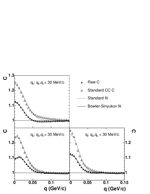
Figure 4: Projections of a three-dimensional correlation function (integrated over 0-30 MeV/c in orthogonal components) for low-$k_{T}$ $\pi^{-}$ pairs for 200 GeV central Au+Au collisions Adams:2004yc (filled symbols) with fit function. Open symbols include correction for Coulomb interaction among all pairs. Projections were generated according to the prescription described in Chacon:1991ri .

For proton-proton correlations and non-identical particle correlations, direct fits are performed by convoluting the full kernel with a parameterized source. For these analyses, the paucity of statistics has been more of a limitation than the relatively modest demands in CPU power. The examples given in Section 4 are all for one-dimensional analyses, but recent data from RHIC will soon be analyzed in multi-dimensions.

The ability to image the source by inverting the kernel is a relatively recent development, but one with very general applications. Because the source is parameterized by a series of B-splines, it is a very general form which is sensitive to non-Gaussian shapes. To date, source imaging has been performed only with one-dimensional correlations, but like with the direct fits, a multi-dimensional kernel will soon be possible Brown:2004bh ; Danielewicz:2005qh .

Non-Gaussian effects were reported in the first pion correlation measurement at RHIC Adler:2001zd . With higher statistics, the STAR Collaboration has studied the issue in greater detail Adams:2004yc , performing a functional expansion (the so-called Edgeworth expansion Csorgo:2003uv ) about a Gaussian shape. Although significant non-Gaussian contributions were reported, the dominant length scales were already extracted in the purely Gaussian fits.

3.5.1 Minimization

A simple chi-squared test is inappropriate for fitting correlation functions because the ratio of two Poisson distributions is not itself Poisson distributed, especially when taking the ratio of small numbers. For this reason, a log-likelihood fit function of the form given in Equation 37 is preferred.

$$\mbox{$\chi^{2}$}_{PML}=-2\left[A\ln\left(\frac{C\left(A+B\right)}{A\left(C+1\right)}\right)+B\ln\left(\frac{A+B}{B\left(C+1\right)}\right)\right],$$ (37)

where A, B, and C were introduced in Equation 35. This equation derived from the principle of maximum likelihood assuming that both signal and background are Poisson distributed Ahle:2002mi . The full derivation of Equation 37 and comparison to earlier log-likelihood functions is given in Ahle:2002mi .

4 Measured Femtoscopic Systematics

The first systematic study to compare femtoscopic measurements across several systems and experiments was performed almost 20 years ago with data from intermediate-energy heavy ion collisions at the Bevalac Bartke:1986mj . The data, taken from experiments with different acceptances, triggers, and analysis techniques, were sufficient to demonstrate a crude $A^{1/3}$ scaling of the one-dimensional radii, indicating that spatial scales were indeed being probed. The first femtoscopic measurements for relativistic heavy ion collisions were presented by the NA35 Collaboration at the Quark Matter meeting in Nordkirchen Humanic:1988ny ; Bamberger:1988kd . More detailed measurements followed with the availability of sulphur and silicon beams at the SPS Boggild:1993zj and AGS Abbott:1992rt ; Barrette:1994pi .

Since then, increasingly sophisticated experiments at the AGS, SPS, and RHIC have performed femtoscopic measurements corresponding to a wide range of control parameters. The experimental community performing the measurements has reached critical mass and matured substantially; a common language and knowledge base has developed concerning sometimes subtle details in performing and interpreting femtoscopic measurements. The result of this effort is a striking degree of consistency across experiments in regions of phase space where acceptances overlap and meaningful generation of systematics across experiments. Large-statistics data sets routinely allow three-dimensional correlation measurements with small statistical error bars. Systematic errors, which now dominate the experimental errors, have been reduced to the level of $\sim 5\%$, or $\sim 0.25$ fm for most measurements. It is no exaggeration to state that femtoscopic measurements have become a precision tool.

Here, we cover the most important systematics of femtoscopic measurements from the AGS, SPS, and RHIC. We discuss only generally the physics probed by a given systematic, appealing to intuitive schematic models such as the blast wave Retiere:2003kf . Full interpretations and comparisons to dynamic models are given in Section 5

4.1 System size: $N_{\rm part}$ and Multiplicity

As discussed earlier, femtoscopic radii probe homogeneity regions, and not the entire source (hereafter, the term source will be used to refer to the entire source of particle emission). Nevertheless, the claim that two-particle correlations probe spatial scales would be given little credence if the radii did not exhibit a strong, positive correlation with system size. Therefore, measuring the systematic variation of the radii vs. system composition and centrality represents the most basic test of both theoretical and experimental femtoscopic techniques.

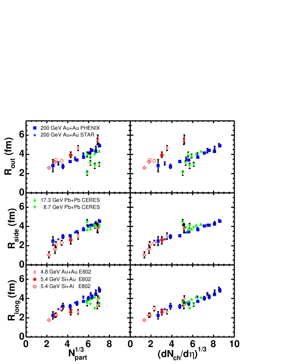
Figure 5: Pion source radius dependence on number of participants (left) and on charged particle multiplicity (right). Data are for for Au+Au (Pb+Pb) collisions at several values of $\sqrt{s_{\rm NN}}$, and also for Si+A collisions at the lowest energy. Average transverse momentum $\langle k_{T}\rangle\sim 450$ MeV/c for the PHENIX data and $\sim 390$ MeV/c for the others. Data from Ahle:2002mi ; Adamova:2002wi ; Adler:2004rq ; Adams:2004yc .

Coalescence studies Barrette:1994tw and two-proton measurements at the AGS Barrette:1999qn and SPS Boggild:1998dx unambiguously demonstrate that nucleon homogeneity lengths increase with decreasing impact parameter and/or increasing projectile mass, continuing the trend mapped at lower energies Lisa:1993xh ; Kotte:2004yv , where directional cuts have allowed measurement of the shape of the homogeneity region Lisa:1993xx ; Lisa:1994xx ; Kotte:1997kz . More detailed information comes from pion correlations at relativistic energies, for which three-dimensional analyses allow partial isolation of purely geometrical effects. The centrality dependence of Bertsch-Pratt source radii are shown in Figure 5 for a wide range of collision energies. The left panels show the dependence on the number of participating nucleons, $N_{\rm part}$, a generalization of the $A^{1/3}$ linear scaling of nuclear radii used to approximate the initial overlap geometry. All of the radii exhibit a linear scaling in $N_{\rm part}^{1/3}$, most with finite intercepts. Only the slope of the $R_{\rm long}$ dependence shows a significant increase from the AGS to RHIC, consistent with a lifetime that increases with both centrality and $\sqrt{s_{NN}}$. The trend of increasing $R_{\rm long}$ with increasing $\sqrt{s_{\rm NN}}$ is reversed for ${\mbox{$\sqrt{s_{\rm NN}}$}}<5$ GeV Lisa:2000no .

The right panels of Figure 5 show the same radii as a function of $(dN_{\rm ch}/d\eta)^{1/3}$. The primary motivation for exploring the $(dN_{\rm ch}/d\eta)^{1/3}$dependence is its relation to the final state geometry through the density at freeze-out. However, the two scaling quantities are highly correlated. In fact, the values of $dN_{ch}/d\eta$ shown on the right side of Figure 5 were derived from $N_{\rm part}$ using the $N_{\rm part}^{\alpha}$ parameterizations given in Adler:2004zn , and conversely, the $N_{\rm part}$ values are often calculated from multiplicity distributions using a Glauber model. Given this caveat, the $R_{\rm side}$ and $R_{\rm long}$values exhibit a linear dependence on $(dN_{\rm ch}/d\eta)^{1/3}$, again with finite intercepts. The strong uniformity from $\sqrt{s_{\rm NN}}$ of 5 to 200 GeV leads one to believe that the approximate $N_{\rm part}$ scaling (initial overlap geometry) is a result of the scaling with multiplicity (final freeze-out geometry) and not the other way around.

The parameter $R_{\rm out}$, which mixes spatial and temporal information (see Section 2.5), increases with multiplicity at each given collision energy, but does not follow a universal curve. However, the strikingly $\sqrt{s_{\rm NN}}$-independent multiplicity scaling of the geometric radii $R_{\rm side}$ and $R_{\rm long}$strongly suggests that the observed increase of these radii with collision energy for $\sqrt{s_{\rm NN}}$ $>$ 5 GeV (see Section 5.1) is due simply to the rise of multiplicity with collision energy. This trend, as well as its violation at $\sqrt{s_{\rm NN}}$ $<$ 5 GeV, has been interpreted in terms of changing chemical composition of the source as the system evolves with energy from baryon to meson dominance Adamova:2002ff .

We note that the systematics in system size represent an initial sanity check for the femtoscopic technique. The obvious direct connection of the radii to the source geometry estimated in two ways refutes suggestions Csorgo:1995bi that smaller, non-geometric length scales dominate experimentally extracted transverse radii.

4.2 Source Shape: Pair emission angle relative to $\hat{b}$

The variation of femtoscopic radii with the pair emission angle relative to $\vec{b}$ ($\phi_{\rm pair}$) can be used to probe the three-dimensional shape of the source Voloshin:1995mc ; Voloshin:1996ch ; Wiedemann:1997cr ; Heiselberg:1998ik ; Heiselberg:1998es ; Lisa:2000ip ; Heinz:2002au ; Retiere:2003kf . The anisotropic shape transverse to the beam direction—the coordinate-space analog to the elliptic flow characterizing momentum-space—gives rise to $\cos(n{\mbox{$\phi_{\rm pair}$}})$ ($n$ even) oscillations in the squared transverse source radii $R_{\rm out}^{2}$, $R_{\rm side}^{2}$, $R_{\rm out,side}^{2}$ Wiedemann:1997cr ; Heinz:2002au .

Just as one expects the source (and homogeneity regions) to be larger for decreasing $|\vec{b}|$, one also expects it to be rounder, reflected by small oscillations of the radii. Figure 7 for mid-rapidity pions from Au+Au collisions at RHIC confirms this expectation. As $|\vec{b}|$ increases, the oscillations indicate a transverse source increasingly elongated out of the reaction plane Adams:2003ra .

The strong in-plane expansion Ackermann:2000tr does not fully convert the initial out-of-plane (overlap) geometry into an in-plane-extended source at freeze-out. This suggests a rather short evolution time; in essence, the system did not have time to reverse its deformation. However, this is only a hint, and a full dynamical transport calculation is required to extract physical timescales Heinz:2002sq .

Whereas at the highest RHIC energy, the freeze-out anisotropy is $\sim\frac{1}{3}$ of the initial Adams:2003ra , at low AGS energies, the final anisotropy is consistent with that of the initial overlap region Lisa:2000xj , or perhaps slightly lower. because elliptic flow vanishes—changes sign—at these energies Pinkenburg:1999ya , these trends make intuitive sense and suggest an underlying connection to the evolution dynamics. It would be desirable to map the source anisotropy at intermediate (AGS and SPS) energies, for which there may be interesting changes in the space-time systematics. At these energies, there have been intriguing hints of asymmetries in the homogeneity regions for pions Miskowiec:1995df ; Filimonov:1999ya ; Nishimura:1999wz ; Aggarwal:2000uj and protons Panitkin:1999yd , and in the proton-pion separation Filimonov:1999ya ; Miskowiec:1998ms , although they have not been finalized.

Figure 6: Squared source radii measured at mid-rapidity in Au+Au collisions at RHIC, as a function of pair emission angle relative to the reaction plane. Data for three centralities are shown. Figure from Adams:2003ra .

Figure 7: Squared source radii measured near mid-rapidity in mid-central Au+Au collisions at lowest-energy AGS settings, as a function of pair emission angle relative to the reaction plane. Figure from Lisa:2000xj .

If the impact parameter direction $\hat{b}$—not simply the $2^{\rm nd}$-order event-plane angle (unambiguous only over a range $[0,\pi]$)—is known, then more detailed information may be obtained. In the left panel of Figure 2, the source is tilted with respect to the beam axis, toward $\hat{b}$. Just as anisotropic azimuthal geometry in the transverse plane is related to the structure of elliptic flow Heinz:2002sq ; Kolb:2003dz , a tilted geometry can reveal important information on the underlying nature of directed flow Csernai:1999nf ; Brachmann:1999xt ; Lisa:2000ip ; Lisa:2000xj . The structure in $R^{2}_{o,l}$ and $R^{2}_{s,l}$ shown in Figure 7 is generated by this tilt. The spatial tilt has been measured only at low AGS energies Lisa:2000xj ; a measurement at RHIC might reveal exotic geometric configurations generated by quark gluon plasma (QGP) formation Brachmann:1999xt ; Magas:2000cm and would impact the important issue of boost-invariance at mid-rapidity.

4.3 Boost invariance : $Y_{\pi\pi}$

In high-energy hadronic collisions, the initial parton distribution is expected to be approximately flat in rapidity. This momentum rapidity distribution may correspond to producing matter that initially exhibits a boost-invariant Hubble-type scaling correlation between longitudinal flow velocity and space-time points, $v_{L,flow}=z/t$ Shuryak:1980tp ; Bjorken:1982qr . Relativistic hydrodynamics preserves boost-invariance of the initial conditions throughout its dynamical evolution Bjorken:1982qr . The combination of the above arguments underlies expectations that in ultra-relativistic heavy ion collisions, particle production emerges from boost-invariant longitudinal flow, and that $dN/dy$ exhibits an approximately boost-invariant plateau around mid-rapidity. However, an extended plateau has never been observed from AGS through RHIC energies Back:2004je .

because correlation measurements access spatio-temporal information, the question arises Wu:1996wk ; Heinz:1996rw whether they allow us to test the relation $v_{L,flow}=z/t$ between the space-time rapidity and the momentum rapidity of the source. For boost-invariant sources, one can show that the pair momentum rapidity is equal to the Yano-Koonin source velocity, which is directly obtained from the Gaussian radius parameters, $Y_{\pi\pi}\approx Y_{L,flow}\equiv\tanh^{-1}v_{L,flow}$. However, even if the source density distribution shows significant deviations from boost-invariance, this relation still holds approximately as long as the velocity profile is boost invariant, and $k_{T}$ is sufficiently large Wu:1996wk .

Figure 8: The Yano-Koonin source rapidity is shown as a function of the pion pair rapidity for central Au(Pb)+Au(Pb) collisions over a broad range of energies (open symbols are for $\pi^{-}\pi^{-}$, closed symbols for $\pi^{+}\pi^{+}$). Both quantities are in the center-of-mass frame of the colliding system. Data from Miskowiec:1996xa ; Appelshauser:1997rr ; Antinori:2001yi ; Back:2004ug .

Figure 8 reveals a roughly universal dependence of ${Y_{\rm YK}}$  on $Y_{\pi\pi}$ for pions from central collisions, depending weakly, if at all, on $\sqrt{s_{NN}}$ (see Section 2.5.3). This trend is particularly striking given the very different center-of-mass projectile rapidities ($\sim 1.55$ and 5.5 for $\sqrt{s_{NN}}=5$ and 200 GeV, respectively) and corresponding widths of the pion distributions $dN/dy$.

By way of caution, we note that the results from RHIC are limited to the region $Y_{\pi\pi}<1.2$, and that the deviations from boost-invariance are mostly in the lower energy data. Extending the RHIC results to more forward rapidities would provide a important test for both the velocity scaling at RHIC and the energy-independence that is exhibited in Figure 8.

For central collisions, the roughly universal behavior approximately obeys the boost-invariant consistency relationship discussed above. Moreover, $Y_{L,flow}$ shows a significant $k_{T}$ dependence and falls below the linear relation in particular for small $k_{T}$  Antinori:2001yi . Qualitatively, this is consistent with blast-wave models in which a boost-invariant longitudinal flow is superimposed on a source density distribution of finite longitudinal width. However, a full dynamical understanding of the dependence is missing so far. The flat ${Y_{\rm YK}}$  dependence on $Y_{\pi\pi}$ measured at the SPS Antinori:2001yi for the most peripheral collisions is counter-intuitive, and requires further study.

The question of whether the source has boost-invariant space-time structure is an important one. There are many reports of very short evolution timescales (lifetimes) based on fits to the data with Equation 24, which is based upon an assumption of boost-invariance Makhlin:1987gm . Relaxation of that assumption might lead to considerably larger estimates Renk:2003gn .

4.4 Collective dynamics: $k_{T}$ and particle mass

As discussed in Section 2.7.2, the dynamic substructure of the source is encoded in space-momentum (${\bf xp}$) correlations. Longitudinal ${\bf xp}$ correlations, encoded in ${\mbox{$R_{\rm long}$}}(k_{T})$, are generally acknowledged Makhlin:1987gm ; Retiere:2003kf to reflect longitudinal flow. because all transverse correlations are generated in the collision itself, considerably more attention has generally been paid to the transverse substructure than to the longitudinal flow discussed in Section 4.3.

The most common explanation for transverse ${\bf xp}$ correlations is collective transverse flow Pratt:1984su . These correlations have mostly been studied through pion correlations, but transverse flow implies also a systematic trend as the particle mass is varied.

4.4.1 $k_{T}$ dependence of pion radii

Figure 9: World data set of published $m_{T}$ dependence of pion Bertsch-Pratt radii near mid-rapidity from Au+Au (Pb+Pb) collisions. Centrality selection is roughly top 10% of cross-section, but varies somewhat with experiment. Data from Lisa:2000no ; Ahle:2002mi ; Adamova:2002wi ; Bearden:1998aq ; Antinori:2001yi ; Aggarwal:2002tm ; Adcox:2002uc ; Adler:2004rq ; Back:2004ug ; Adler:2001zd ; Adams:2004yc Lines represent parameterized fits; see text for details.

Collective flow generates a characteristic fall-off of the pion source radii with $k_{T}$, which is ubiquitously observed in data. Final results for the $k_{T}$-dependence of Gaussian radii from central Au+Au (Pb+Pb) collisions exist at the AGS Lisa:2000no ; Ahle:2002mi , SPS Appelshauser:1997rr ; Bearden:1998aq ; Aggarwal:2002tm ; Antinori:2001yi ; Adamova:2002wi , and RHIC Adler:2001zd ; Adcox:2002uc ; Adams:2003ra ; Adams:2004yc ; Back:2004ug ; Adler:2004rq . As is clear from Figure 9, aside from a small variation in overall scale (discussed later), the $k_{T}$ dependence is startlingly similar for all energies.

Figure 11 quantifies the evolution of the $m_{T}$-dependence of the pion source radii with $\sqrt{s_{\rm NN}}$, using fits to $R_{i}(m_{T})\sim m_{T}^{-\alpha_{i}}$. As discussed in Section 2.7.1, $\alpha_{i}=0.5$ would represent expectations for instantaneous thermal emission for a three-dimensionally expanding fireball in the limit of large $m_{T}$.

The similarity persists as $N_{\rm part}$ is varied. In Au+Au collisions at RHIC, $R_{i}(m_{T})$ ($i={\rm out,side,long}$) simply scale as $N_{\rm part}^{1/3}$, with perhaps some flattening for ${\mbox{$N_{\rm part}$}}<100$ Adams:2004yc ; Adler:2004rq . Very similar $k_{T}$ dependence for different $N_{\rm part}$ is also observed in Pb+Pb collisions at SPS Adamova:2002wi and for Si+Au and Au+Au collisions at the AGS Ahle:2002mi .

In a flow-dominated freeze-out scenario, the fall-off of transverse radii with $m_{T}$ increases as flow increases and/or temperature decreases (e.g. Retiere:2003kf, ). Blast-wave fits to spectra Xu:2001zj indicate that freeze-out flow and temperature vary significantly with $\sqrt{s_{\rm NN}}$ for ${\mbox{$\sqrt{s_{\rm NN}}$}}\lesssim 10$ GeV. The overall approximate $\sqrt{s_{\rm NN}}$-independence of the $\alpha_{i}$ parameters may reflect the fact that significantly changing the slope of $R_{i}(m_{T})$ requires very large changes in flow and temperature; on the other hand, it could be that the compensating effects of smaller (larger) homogeneity lengths generated by larger flow (temperature) cancel almost exactly in nature. Although $R_{i}(m_{T})$ almost certainly reflects strong collective flow, determining the strength of that flow requires other information, such as particle spectra Lee:1990sk ; Retiere:2003kf .

because the radii fall off roughly as $1/\sqrt{m_{T}}$ (see Figure 11) and such a dependence has been discussed frequently in the literature (e.g. Beker:1995qv, ; Csorgo:1996no, ), it is interesting to look at the overall scale parameter from a single-parameter fit to $R^{\prime}_{i}/\sqrt{m_{T}}$. The $\sqrt{s_{\rm NN}}$-dependence of $R^{\prime}_{\rm side}$ and $R^{\prime}_{\rm long}$ are shown in Figure 11. The scale of the longitudinal homogeneity length grows significantly with $\sqrt{s_{\rm NN}}$, consistent with an increase of the system evolution time. However, $R^{\prime}$ varies only very weakly with $\sqrt{s_{\rm NN}}$.

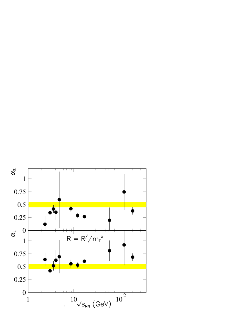
Figure 10: The excitation function of $m_{T}$ power-law fall-off of pion source radii ($R_{i}(m_{T})\sim m_{T}^{-\alpha_{i}}$). Shaded regions show $\alpha_{i}=0.5\pm 0.05$.

Figure 11: The excitation function of scale parameters $R^{\prime}_{i}$ from fits of the data in Figure 9 to $R_{i}(m_{T})=R^{\prime}_{i}/\sqrt{m_{T}}$. Note: this is a different functional form than that used in Figure 11.

4.4.2 Systematics with particle mass

Systematic studies for different mass particles provide additional controls probing the space-time evolution of the source. In particular for kaons, the interpretation may be simplified owing to reduced effects of resonance feed-down Gyulassy:1989pp and a reduced scattering cross-section for $K^{+}$ in nuclear matter, raising the possibility that kaon correlations could peer farther back to earlier stages of the collision Schnetzer:1982ga . Indeed, the first kaon measurements Akiba:1993cj ; Beker:1994qs ; Cianciolo:1995dd ; Miskowiec:1996xa reported smaller source radii for kaons. However, the observation that radii for $K^{+}$ and $K^{-}$ were very similar Beker:1994qs was an early experimental indication that different cross-sections were not the driving physics behind these smaller radii. This was supported by model calculations Sorge:1989vt , which suggested that $K^{+}$ and $K^{-}$ in fact scattered roughly equally in the dense medium created in heavy ion collisions. In this case, the smaller radii for kaons results from their increased mass in a flow field, not different cross-sections.

If indeed flow is generated in matter sufficiently dense that individual cross-sections are unimportant, then all particles participate equally in collective transverse flow. In this case, their source radii should approximately follow a common $m_{T}$ scaling Akkelin:1995gh ; Csorgo:1995bi ; Wiedemann:1995au ; Wiedemann:1999qn . Within uncertainties, first results on kaon interferometry by NA44 at the SPS in S+Pb Beker:1995qv and Pb+PB Bearden:2001sy collisions were consistent with a $1/\sqrt{m_{T}}$ scaling expected for isotropic Hubble flow Akkelin:1995gh ; Csorgo:1995bi ; Wiedemann:1995au . In some more recent analyses Afanasiev:2002fv , the common $m_{T}$ systematic for the transverse radii is less steep than for ${\mbox{$R_{\rm long}$}}(m_{T})$ (see Figure 11), as might be expected for more boost-invariant (non-isotropic) flowing systems Wiedemann:1999qn ; Retiere:2003kf .

Figure 12 collects the $m_{T}$ dependence of homogeneity lengths for several energies. The left panels show results for Si+Au collisions at $\sqrt{s_{\rm NN}}$=5.4 GeV, measured by E802 for pions Ahle:2002mi and kaons Akiba:1993cj ; Cianciolo:1995dd . Femtoscopic radii for pions Bearden:1998aq ; Afanasiev:2002fv ; Adamova:2002wi ; Aggarwal:2002tm kaons Bearden:2001sy , protons Appelshauser:1999in , and photons Aggarwal:2003zy measured in Pb+Pb collisions at the SPS are shown in the center panels. The right panel shows the one-dimensional radius parameter $R_{\rm inv}$ measured at RHIC for pions, charged kaons, and protons Heffner:2004js , neutral kaons Bekele:2004ci , and with $\Lambda-p$ correlations Renault:2004pp . To compare across energies, $R_{\rm inv}$ results are included for the AGS and also for the SPS, where the $R_{\rm inv}$ values were calculated from the 3D fit results by accounting for the boost along the outwards direction from the LCMS (in which $P_{z}=0$) to the PCOM (pair center-of-mass, in which $\mid\stackrel{{\scriptstyle\rightharpoonup}}{{P}}\mid=0$) frame, $R_{\rm inv}^{2}=R_{\rm long}^{2}+R_{\rm side}^{2}+\gamma^{2}R_{\rm out}^{2}$, where $\gamma$ is given by $m_{T}/m$ of the pair. Note that for massless particles, such as photons, $\gamma$ is given by $k_{T}/Q_{\rm inv}$. For a given orientation of the photon pair momentum $R_{\rm inv}$ can be related to 3D radii in the LCMS frame through the following expression for the exponent of the Gaussian source term,

$$Q^{2}_{\rm inv}R^{2}_{\rm inv} = Q^{2}_{\rm inv}\left(R^{2}_{\rm long}\cos^{2}\theta+R^{2}_{\rm side}\sin^{2}\theta sin^{2}\phi+k^{2}_{T}/Q^{2}_{\rm inv}R^{2}_{\rm out}\sin^{2}\theta cos^{2}\phi\right)$$ (38)

$$= k^{2}_{T}R^{2}_{\rm out}\sin^{2}\theta cos^{2}\phi+Q^{2}_{\rm inv}\left(R^{2}_{\rm long}\cos^{2}\theta+R^{2}_{\rm side}\sin^{2}\theta sin^{2}\phi\right).$$

Thus $R_{\rm out}$ drops completely out of the source term and enters into the $\lambda$ coefficient Aggarwal:2003zy , but as a function of $k_{T}$. For this reason the 1D $Q_{\rm inv}$ fits from WA98 are plotted alongside values of $R_{\rm side}$ and $R_{\rm long}$ instead.

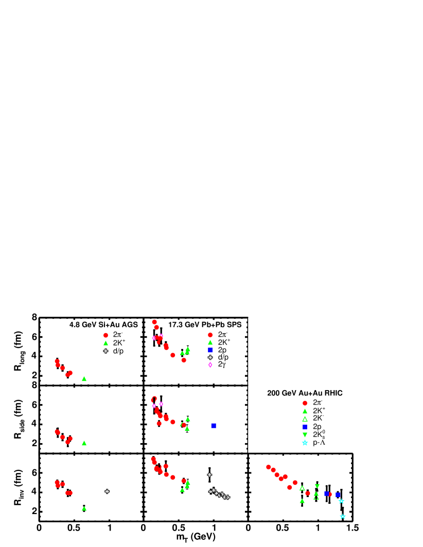
Figure 12: Transverse mass dependence of homogeneity lengths from correlations between particles of (nearly) identical mass.

This consistency between different particle types may carry an important message. It calls into question theoretical scenarios which appear to explain $R_{i}(m_{T})$ for particular particle types only Cramer:2004ih . Further, the consistency with emission from a common flow-dominated source may also support freeze-out scenarios in which the last scattering in the dense phase determines the homogeneity region, instead of milder rescatterings in the more dilute stage, which are dominated by particle species-dependent cross-sections Kapusta:2004ju ; Wong:2004gm .

4.5 New possibilities: Non-identical particle correlations

Almost all femtoscopic measurements to date have been done through correlations of identical particles, usually charged pions. With the availability of high-statistics data sets and new theoretical ideas Lednicky:2001qv , however, experiments are beginning to make full multi-dimensional analyses of non-identical particle correlations. These correlations are being used to test and refine the treatment of Coulomb effects in identical-particle correlation analyses, to explore violations of flow-induced universal $m_{T}$ scaling, and to extract qualitatively new information on the space-time substructure of the source.

4.5.1 Opposite-sign pion correlations

The most common non-identical particle femtoscopy measurements have involved $\pi^{+}-\pi^{-}$ correlations. Here, the natural assumption is that the homogeneity regions of these particles coincide. The primary interest is in whether the homogeneity volume is extracted from $\pi^{\pm}-\pi^{\pm}$ correlations—driven by quantum statistics and Coulomb final state interactions (with minimal strong FSI effects)– is consistent with that extracted from $\pi^{+}-\pi^{-}$ correlations—determined only by Coulomb and strong FSI Adams:2004yc . This issue has obvious implications for the FSI weight $F({\bf q})$ discussed in Section 3.5.

At the SPS, $\pi^{+}-\pi^{-}$ correlations from reactions with sulphur Alber:1997av and lead Appelshauser:1997rr beams were consistent with emission from a homogeneity region with spatial scale roughly the same as the radii from identical-particle correlations. Preliminary analysis of opposite-sign pion correlations from Au+Au collisions at the AGS Miskowiec:1996xa ; Miskowiec:1998ms similarly find consistency with scales extracted from like-sign pion correlations. Recently, STAR reported Adams:2004yc strong consistency at RHIC energies as well. Using large-statistics data sets, they further show that contributions to the $\pi^{+}-\pi^{-}$ correlation function from strong-force interactions, though small, are nevertheless important in explaining the data in detail.

4.5.2 Other non-identical particle correlations in $|\vec{q}|$

For statistical reasons, most non-identical particle correlations are measured in one-dimensional $|\vec{q}|$-space, and thus probe only the average spatial separation between the two particles at freeze-out in the pair center-of-momentum frame (see Section 2.3). Because they are sensitive to the size of each particles emission source and this separation between them, it is often necessary to rely on the identical particle correlations for a proper interpretation of results.

Despite these ambiguities, one-dimensional non-identical particle correlations may be used to test existing systematics and expectations of the freeze-out scenario. Conversely, if the freeze-out geometry may be taken as given, non-identical particle correlations may place constraints on hadronic scattering parameters, e.g. to measure the squared relative wave-function of a pion and a $\Xi$ baryon. First studies along these lines are underway at RHIC Renault:2004me .

Wang and Pratt Wang:1999bf suggested the measurement of $p-\Lambda$ correlations, which may be more sensitive to large structure than $p-p$ correlations, and which have a higher two-track reconstruction efficiency for some experiments. Published results from Au+Au collisions at the AGS Chung:2002vk suggest a $p-\Lambda$ separation distribution with a width similar to the proton homogeneity length and roughly consistent with $m_{T}$ scaling expectations (cf Section 4.4.2). Preliminary results at SPS Blume:2002mr and RHIC Renault:2004me ; Kisiel:2004it give similar conclusions. because the $p-\Lambda$ potential is not unambiguously known theoretically Wang:1999bf , it is unclear whether possible statistically marginal violations of $m_{T}$ scaling Chung:2002vk or differences between baryon and anti-baryon emission regions Renault:2004me are meaningful. To first order, existing $p-\Lambda$ correlations confirm existing systematics.

With the high-statistics and high-quality data sets at the largest collision energies, truly exotic correlation studies are possible. Preliminary results Kisiel:2004it from RHIC on $\pi-\Xi$ correlations look particularly promising. Here, the well-measured pion emission distribution may be used to study the strange baryon freeze-out configuration. It may also provide information on the $\pi-\Xi$ final state interaction and scattering cross-section which in turn can be used to constrain our understanding of the sources of collective flow. Blast-wave calculations reproduce the preliminary $\pi-\Xi$ correlations, suggesting that the $\Xi$ flow is determined by its mass, not its quark content.

4.5.3 New information: non-identical particle correlations with directional cuts on $\vec{q}$

Non-identical particle correlation analyses as a function of—or with cuts on—the relative direction of $\vec{q}$ and $\vec{P}$ reveal qualitatively new information (Lednicky:1995vk, ; Voloshin:1997jh, ; Lednicky:2001qv, , and Section 2). In particular, in addition to the root mean square (RMS) width of the separation distribution, the direction and size of the average separation between the particles is probed, although offsets in time and space cannot be disentangled; this is shown as $\Delta r$ in Figure 3. The correlation functions selected for $\vec{q}\parallel\vec{P}$ and $\vec{q}\nparallel\vec{P}$ differ if $\Delta r\neq 0$. Furthermore, collective flow will induce position-momentum correlations detectable with directionally selected non-identical particle correlations Voloshin:1997jh ; Retiere:2003kf .

These correlations are statistically challenging, and few results are available. At RHIC, STAR has reported Adams:2003qa asymmetries in $K^{\pm}-\pi^{\pm}$ correlations measured in central Au+Au collisions. Blast-wave calculations with transverse flow roughly adjusted to reproduce other observations at RHIC Retiere:2003kf describe the data semi-quantitatively. Preliminary studies of $p-\pi$ correlations at the SPS Blume:2002mr and RHIC Kisiel:2004it exhibit similar mass-ordered spatial asymmetries in the transverse plane. A preliminary study at the AGS Miskowiec:1998ms reported very large ($\Delta r_{\rm long}\approx$ 10 fm) average $p-\pi$ separations in the longitudinal (beam) and impact parameter direction for forward-moving particles, suggesting strong longitudinal flow; however, this result was never confirmed.

We expect full three-dimensional analyses of a wide range of non-identical particle combinations to be available in the near future from RHIC experiments. Sophisticated analyses may probe non-trivial geometric substructure when selecting on reaction plane, including the sideward shift predicted by blast-wave calculations Retiere:2003kf when anisotropic flow structure is present.

5 Interpretations of Experimental Results

In this section, we ask what we can learn from the spectrum of results just presented. Beginning with the broadest, least detailed observations, we move to two fundamental quantities that may be directly extracted from the data, and finally on to comparisons with specific models of heavy ion collisions.

5.1 General Conclusions from Systematic Trends

One of the first messages to take away from the discussion of Section 4 is that the results are stable across detector and method; experimental systematics and uncertainties are under control. Whatever difficulties we may have in interpreting measurements, we may be confident that they do not have their origin in experimental artifact.

The size and shape inferred from two-particle correlations tracked with collision geometry as anticipated. Kinematic and mass dependences of femtoscopic measurements showed the expected clear signatures of strong collective flow in the beam direction and perpendicular to it.

At a generic level (ignoring quantitative predictions), we are first given pause at the jejune nature of the $\sqrt{s_{NN}}$-dependence of femtoscopic parameters. The most common example discussed is the pion source radii excitation function shown in Figure 13. In Section 4 we explored the trends in considerably greater detail, but the figure conveys the right message: Scanning $\sqrt{s_{NN}}$ through a range of two orders of magnitude changes final-state geometry little.

Based on rather generic arguments of soft points in the equation of state or entropy generation during a phase transition, there had been hopes for non-trivial structure in the excitation function, as the energy threshold for quark gluon plasma (QGP) creation was crossed Pratt:1986cc ; Bertsch:1988db ; Rischke:1996em ; Harris:1996zx . General expectations were for long (relative to the explosion of a purely hadronic system) system evolution time scales if QGP was formed. Blast-wave analyses of data (e.g. Retiere:2003kf, ) appear to rule out systems with lifetimes in the neighborhood of 20 fm/c or higher. However, owing to dynamic effects, careful comparison with a dynamical model is required to extract detailed evolution information; this is discussed in Section 5.3.

As discussed in Section 4.1, the weak increase with $R_{\rm out}$of the femtoscopic radii for central collisions shown in Figure 13 is mostly due simply to increasing multiplicity. The CERES collaboration Adamova:2002ff . has suggested that this increase may be understood in terms of an energy-independent mean free path of 1 fm at freeze-out. Interestingly, this explanation also appears to describe the decrease of radii with ${\mbox{$R_{\rm out}$}}~{}<5GeV$, when the different cross-sections and abundances of pions and protons are accounted for. This observation emphasizes the importance of chemistry in the determination of the freeze-out geometry. However, it neglects the dynamical structure of the source (e.g., flow) and the importance of the six-dimensional phase space density discussed in Section 2.9. We discuss this fundamental quantity next.

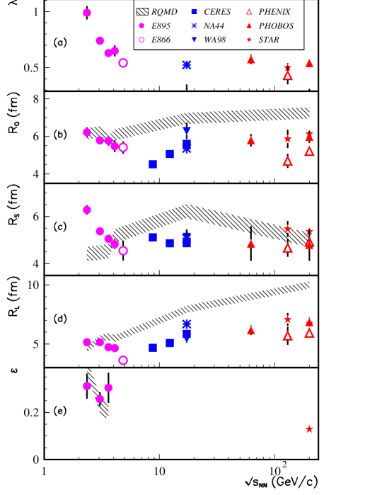
Figure 13: Panels (a-d): Excitation function of $\pi^{-}$ source parameters at mid-rapidity and low $k_{T}$ ($\sim 0.17$ GeV/c) in central Au+Au(Pb+Pb) collisions. PHENIX data are for $k_{T}\sim 0.26$ GeV/c and so fall somewhat below the trend. Panel (e): Transverse freeze-out anisotropy parameter from non-central ($|\vec{b}|\sim 8$ fm) Au+Au collisions, estimated from the azimuthal dependence of source radii. Data are from Adcox:2002uc ; Adler:2004rq ; Adler:2001zd ; Adams:2003ra ; Adams:2004yc ; Ahle:2002mi ; Adamova:2002wi ; Aggarwal:2002tm ; Back:2004ug ; Bearden:1998aq ; Lisa:2000no ; Lisa:2000xj . Also shown are calculations Lisa:2000no ; Lisa:2000xj ; Bearden:1998aq ; Hardtke:1999vf at several energies with the RQMD model Sorge:1995dp ; hashed region at other values of $\sqrt{s_{NN}}$ interpolates between these calculations.

5.2 Phase Space Density and Entropy

As shown in Section 2.9, average phase space densities, $\bar{f}({\bf p})$, can be calculated by combining source-size measurements with spectra. Pionic phase space densities have been estimated for 130$A$ GeV collisions at RHIC Pal:2003rz , at the top SPS energies, and for several AGS energies Lisa:2001fw . Figure 14 shows results for all three regions. In each case, the phase space densities were calculated via Equation 28. For the SPS case, results were generated by applying Equation 28 to published spectra Afanasiev:2002mx and source-size measurements Kniege:2004pt . We note that our calculations for the SPS are higher than previously published values at low $p_{t}$ Ferenc:1999ku . This discrepancy is likely due to the fact that in Reference Ferenc:1999ku , analytic parameterizations were used that differ significantly from published spectra at low $p_{t}$.

When applying Equation 28, an issue arises as to whether one should subtract the contribution from resonances to the spectra. Indeed, if the pions are created by decays so far outside the source volume that they do not contribute to the correlation function, they should not be considered as pions when calculating the phase space density. There are two strategies to correct for such pions. First, one could use spectra where such particles are subtracted and apply Equation 28 literally. As a second option, one could use the spectra without subtractions, but then multiply the expression for $\bar{f}$ by $\sqrt{\lambda}$. because most published spectra have been purged of the products of weak decays, the first method is usually applied. However, published spectra still include the contribution from $\eta$’s, which decay thousands of fm away from the source. The $\eta$ contribution was accounted for in the SPS calculation for Figure 14 by reducing the spectra by 5%.

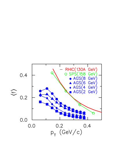
Figure 14: Average pionic phase space densities for central Au+Au and Pb+Pb collisions from the AGS to RHIC rise with beam energy but seem to plateau at SPS energies. Values were calculated with Equation 28.

The phase-space densities in Figure 14 show a steady rise with beam energy that seems to plateau at SPS energies. because the displayed phase space densities have been averaged over coordinate space, the peak values are higher Tomasik:2001uz ; Tomasik:2002qt , by a factor of $2\sqrt{2}$, if the spatial profiles are Gaussian. For a breakup temperature of 110 MeV, this requires a rather high chemical potential, near or above 80 MeV Greiner:1993jn ; Pratt:1999ku ; Akkelin:2004he .

Ratios of particle yields are consistent with chemical freeze-out at temperatures near 170 MeV Braun-Munzinger:2003zd ; Braun-Munzinger:2001ip ; Andronic:2003zv . This suggests an interpretation where at higher densities the system is so strongly interacting that yields equilibrate until the system reaches this temperature and are then frozen during the subsequent freeze-out. At AGS energies, the increase in pion production brought on by increased beam energy results in more pions being pushed into a given amount of phase space as realized in Figure 14 by the rising phase space density. However, one would expect that as the excitation energy surpasses the threshold for a 170 MeV temperature, the phase space density would reach a limiting value. because the average phase space density is preserved in an isentropic expansion with fixed particle number (not exactly true if several masses are mixed together), one would expect phase space densities to saturate once energy densities reached this value. Indeed, the behavior in Figure 14 is consistent with this scenario.

As shown in Section 2.9, entropy can be calculated from average phase space densities using Equation 30. Spectra and source-size measurements for baryons and mesons were used to estimate phase space densities and entropy for 130$A$ GeV Au+Au collisions at RHIC. The total entropy in the central unit of rapidity was estimated at $dS/dy=4450\pm 10\%$ Pal:2003rz . In a hydrodynamic expansion, entropy is conserved though viscosity, and shock waves might result in a roughly 10% increase during the evolution. Thus, this measurement provides an upper bound for the entropy at $\tau\sim 1$ fm/c when thermalization first occurs. At $\tau=1$ fm/c, the volume for particles in this rapidity slice is determined by the geometric cross-sectional areas of the overlapping gold nuclei multiplied by $c\tau$, thus an upper bound for the entropy density can be determined $s\leq(dS/dy)/(\tau\pi R^{2})$. Knowing the energy density at $\tau=1$ fm/c would then provide a point in the equation of state, $s$ vs. $\epsilon$. The value of $dS/dy$ estimated in Pal:2003rz is consistent with lattice calculations if $\epsilon(\tau=1~{}{\rm fm/c})\sim 7$ GeV/fm³. Estimates of the original energy density from the final-state measurement of $dE_{t}/d\eta$ are in the range of 4.5 GeV/fm³ Adcox:2001ry , but because these estimates neglect losses from longitudinal work or the energy from longitudinal thermal motion, the 7 GeV/fm³ value seems reasonable.

5.3 Dynamic Models and their Comparison with Data

It is increasingly recognized that the comparison of dynamic models of heavy ion collisions to data is only insightful if it involves a sufficiently large variety of experimental data. A comparison of dynamic models to femtoscopic measurements alone (or to any other class of measurements alone) is of limited value, simply because for realistic models, the number of possible model-dependent parameter choices then tends to exceed the number of experimental constraints. In fact, all the model results that we review in the current subsection remain unsatisfactory with this respect: They either deviate significantly from femtoscopic data, or they reproduce these data at the price of missing other important experimental information. In particular, there is so far no dynamically consistent model that reproduces quantitatively both the systematic trends discussed in Section 4 and the corresponding single inclusive spectra. In this situation, the scope of this subsection is somewhat limited. We want to explain why a dynamical understanding of femtoscopic measurements is important. We shall also discuss the key physics input that enters current attempts of dynamic modeling and the uncertainties resulting from it. However, we shall try to bypass as far as possible model-dependent details and rather focus on the question of which qualitative changes in the underlying dynamics result in characteristic changes of femtoscopic data.

Correlation measurements provide a snapshot of the geometrical distribution of particles at the time they decouple from the reaction. This geometrical distribution provides a unique test of the dynamical evolution of the produced matter at the late stage. because the spatial extension, dynamical evolution, and lifetime of the produced system determines phase space density and thus particle reaction rates, any dynamic model for the latter has to be consistent with femtoscopic information. So far, correlation analyses have focused mainly on Boltzmann (or cascade) models, on hydrodynamic models, or on combinations of both (hybrid models). These model classes correspond to rather different equations of state.

The equations of state represented by cascade models tend to be stiff unless they incorporate large number of resonant scatterings. If particles collide via $2\rightarrow 1\rightarrow 2$ processes where the intermediate state has a finite lifetime, the equation of state can be softened Danielewicz:1995ay ; Larionov:2001zg . A prominent example of a cascade model is RQMD Sorge:1989vt , Relativistic Quantum Molecular Dynamics; it is the only one which has been compared to data at AGS, SPS, and RHIC. Results for RQMD are shown in Figure 13. However, for RHIC energies, the dynamic consistency of RQMD is questionable because for most of its evolution, the model uses hadronic degrees of freedom, although RQMD simulations for RHIC yield an energy density which stays above that of normal nuclear matter for a significant duration ($\sim 5$ fm/c). As can be seen in Figure 15, RQMD, which models the expansion as a hadronic cascade, overpredicts $R_{\rm out}$ and $R_{\rm long}$ at RHIC despite the fact that it underpredicts multiplicities. Another hadron cascade model, the Hadronic Rescattering Model Humanic:2002iw ; Humanic:2003gs , based solely on hadronic rescattering with sudden collisions, gives smaller sources, which come closer to the data. Part of the difference between the two hadronic cascades may derive from RQMD’s treatment of scatterings as resonant interactions with finite lifetimes, which differs from the instantaneous collisions employed in the Hadronic Scattering Model. Figure 15 also displays results for Molnar’s Parton Cascase (MPC) Molnar:2002bz , which aims to provide a transparent partonic toy model by modeling the collision of light partons which undergo a one-to-one hadronization to pions. MPC, which has only instantaneous two-to-two scatterings, should have the stiffest effective equation of state and underestimates the source radii.

On of the most complicated transport codes available is A Multi-Phase Transport (AMPT) model. AMPT Lin:2002gc ; Lin:2003iq aims at a realistic description of all aspects of the reaction dynamics and includes a partonic cascade coupled to a hadronic cascade employing a full list of resonant interactions. AMPT provides a good fit to experimental radii, though the $k_{T}$ fall-off is stronger than that found in the data, which fall off $\sim m_{T}^{-1/2}$. The more rapid decrease of radius parameters with respect to $k_{T}$ may be due to the continuous surface-like emission characteristic of microscopic models, which when combined with cooling gives a higher relative weight for high-energy particles to have been emitted earlier in time, before the reaction volume has reached its full spatial extent. Any modification that would reduce this type of emission should improve agreement with data. Cautiously, one would conclude that the results in Figure 15 favor models with a stiff, but not too stiff, equation of state and no latent heat.

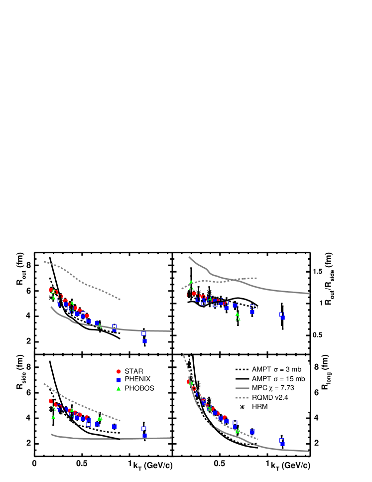
Figure 15: Pion radius parameters from four Boltzmann/cascade models are compared to experimental RHIC data. For Molnar’s Parton Cascase calculations, the reported radii are simply space-time variances. For the other models, radii are obtained from Gaussian fits to correlation functions generated according to the methods described in Section 2.8. Measured data for positive and negative pions are indicated by closed and open symbols, respectively.

This conclusion is further supported if one compares the results of cascade models with those of hydrodynamic simulations or hybrid models. Figure 16 compares results from RHIC to a three-dimensional hydrodynamic model of Hirano et al. Hirano:2002ds that investigates the effects of resonance decays on chemical composition, the two-dimensional model of Heinz and Kolb Heinz:2002un , and a two-dimensional chiral model by Zseische et al. Zschiesche:2001dx that performs calculations for both first order and cross-over transitions. In all cases, the more favorable calculations are compared with the data: partial chemical freeze-out for Hirano, and cross-over transition for Zschiesche, but large discrepancies between the models and the data still remain. The results from Zseische were taken from the cross-over transition for the lowest critical temperature, 80 MeV. Substituting a first order phase transition or increasing the critical temperature to 130 MeV increased the value of $R_{\rm out}$ relative to $R_{\rm side}$, thereby increasing the differences with the data. Hirano also reported a calculation under complete chemical equilibrium at freeze-out; this improves the agreement with v₂, but at the expense of a much larger value of $R_{\rm out}$/$R_{\rm side}$.

In general, these models invoke equations of state that are typically softer than those used in cascades and Boltzmann calculations, and they often have latent heats to accompany the transition from the partonic phase. As a consequence, lifetime and emission duration of the produced matter are significantly larger than what one finds in cascade models, and such models often significantly over-predict $R_{\rm long}$ and $R_{\rm out}/R_{\rm side}$. The fact that $R_{\rm side}$ comes out smaller than the data in Figure 16 is mainly due to an attempt to compensate within the available model-parameter range the very large time-scales as much as possible. Purely hydrodynamic models can vary overall source volumes by adjusting the break-up criteria, but doing so can make it difficult to fit the three source dimensions, and their $m_{T}$ dependence, as well as other observables. Several prescriptions have been applied to improve the modeling of the breakup in the late stage to depend on microscopic considerations determined by free-space cross-sections without having an extra adjustable parameter, e.g. break-up density, Csernai:2004pr ; Sinyukov:2002if ; Tomasik:2002qt . An alternative to improve the description of breakup is the use of hybrid models, in which hydrodynamic evolution in the early stage is combined with cascading in the late stage. In Figure 16, we compare results of one such hybrid model, Ultrarelativistic Quantum Molecular Dynamics (URQMD) Soff:2000eh ; Bass:2000ib , to results of hydrodynamic calculations. Similar results were obtained by Teaney et al. Teaney:2001gc ; Teaney:2001av . Compared to hydrodynamic simulations, hybrid descriptions do not seem to notably reduce the overpredicted lifetimes. They tend to emit most of the pions at a time near or above 15 fm/c and significantly overpredict $R_{\rm out}/R_{\rm side}$ ratios, whereas blast-wave parameterizations favor breakup times near or slightly below 10 fm/c. However, firm conclusions that the relative failure of hybrid models derives from the chosen equations of state cannot be made until comparisons are made between Boltzmann and hybrid calculations that use the same equation of state. Until such an analysis is performed, other issues will cloud the interpretation, such as whether viscous effects or details of the hydrodynamic/Boltzmann interface dominate results and might even invalidate the hydrodynamic approach.

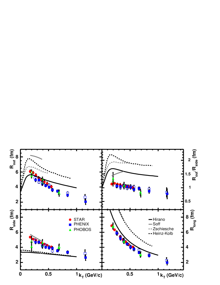
Figure 16: Hydrodynamic (Zschiesche, Hirano, and Kolb) and hybrid hydrodynamic/cascade (Soff) models calculations in comparison to RHIC data. Data are for 2$\pi^{-}$(open symbols) and 2$\pi^{+}$(closed symbols) source radii.

Entropy and pressure are intimately related, in that knowing the entropy density as a function of the energy density determines the pressure as a function of energy density. Whereas one can intuitively understand why a lower pressure would lead to longer lifetimes and larger source dimensions, the manifestations of changing the entropy are less transparent. One way to understand the effects of changing the entropy is to associate higher entropy with a larger effective number of light degrees of freedom. For instance, if one were to hadronize via a one-to-one parton-to-pion scheme, the volume per identical particle would change by a factor of the number of degrees of freedom. If the r.m.s. momentum is the same before and after hadronization, this would imply a change in entropy per particle equal to the logarithm of the ratio of effective degrees of freedom, and if $\sim 40$ light partonic degrees of freedom were immediately replaced by three pionic degrees of freedom, the system would lose $\ln(40/3)$ units of entropy per particle. To conserve entropy, a system must expand its volume by a similar ratio which implies an increase in radius parameters. Hydrodynamic models, which manifestly conserve entropy, use the energy stored in the latent heat to provide the heat necessary to preserve entropy during hadronization. Entropy conservation is more difficult to enforce in microscopic approaches. This underlines the challenges involved in applying microscopic simulations in an environment of strongly interacting matter with ill-defined degrees of freedom, and it re-emphasizes the importance of gaining a better understanding of the validity of hydrodynamic calculations in such manifestly finite situations. It is peculiar that the entropy extracted from source-size and spectral measurements is consistent with the lattice-inspired equation of state Teaney:2001gc ; Teaney:2001av , whereas the source sizes extracted from hybrid models incorporating similar equations of state significantly overpredict source sizes. Part of this contradiction can be explained by increases in the populations of baryons, which, because they inherently have more entropy per particle than do pions, can account for much of the missing entropy Pal:2003rz . Thus, the HBT puzzle does not necessarily imply an entropy puzzle.

The HBT puzzle is not so much that radius parameters cannot be fit by models, but that our most sophisticated models, which incorporate a phase transition, fail to reproduce the data. The very gradual evolution of extracted source sizes as beam energies traverse a large range of energies is remarkable and puzzling in its own right. A simple explanation is that the equations of state do not dramatically change as the energy density changes from hadronic to super-hadronic densities, i.e., there is not even a hint of a latent heat. In fact, the failure of hydrodynamical models to reproduce femtoscopic measurements might be largely due to unrealistically large latent heats needed to reproduce elliptic flow data Pasi . However, as emphasized above, a host of unresolved issues prevent more quantitative conclusions. These qualifiers cannot be lifted until much more thorough analyses of models are performed that entail a systematic exploration of the sensitivity of model predictions to both parameters and assumptions. This would necessitate a tremendous commitment from the community, but without it, many conclusions about the matter created in relativistic heavy ion collisions will remain vague.

6 Summary

Twenty-five years ago, the goal of femtoscopy was to demonstrate that one could measure a hadronic length scale with correlations, and if a result was on the order of a few Fermi, the analysis was deemed a success. In contrast, with the improved accuracy of measurements, the enormous increase in statistics, and the simultaneous development of phenomenology and theory, femtoscopy is now considered a precision measurement. Ten percent deviations between theory and experiment are now taken seriously as evidence that the spatio-temporal description of a model is significantly flawed. At RHIC energies, all six dimensions of the correlation function have been exploited to provide truly three-dimensional insight into the phase space cloud for particles of any momentum with any direction.

For relativistic heavy ion collisions, there were expectations that a transition from hadronic to partonic matter might be accompanied by a large latent heat, which would bring about a dramatic change in the dynamics as beam energies traversed the range for exploring the mixed phase. Within this range, it was expected that the latent heat and the associated softening of the equation of state would manifest itself by slowing the explosion with lifetimes approaching or exceeding 20 fm/c. The signal of the phase transition would have been an increase of the effective lifetime for a range of beam energies followed by a return to more explosive and shorter-lived reactions at even higher energies.

Extended lifetimes were not observed. Increasing beam energies from AGS to RHIC indeed causes larger energy densities and higher multiplicities, which push toward increasing the source volumes. However, much of this increase in multiplicities is absorbed by higher phase space densities rather than larger source sizes. Combined with the increasing strength of radial flow, which provides smaller regions of homogeneity relative to the overall source volume, the result is that the effective dimensions change remarkably little over a wide range of beam energies. Furthermore, it appears that lifetimes of the reaction never leave the neighborhood of 10 fm/c. Not only does this represent a lack of evidence for a latent heat, it also suggests that there is no such latent heat.

These conclusions remain only modestly guarded. Theory and phenomenology are progressing, but improvements in such aspects as mean-field effects or accounting for the smoothness approximation are not expected to change conclusions by more than 10%. As with the improvements in including Coulomb effects in Section 4, removing some of the distortions and aberrations from the analyses is likely to be significant for fine-tuning models, but should not alter the conclusion that there is no large latent heat associated with the reaction.

The theory of modeling, i.e., generating the source functions, has the greatest need for progress. because femtoscopic measurements are determined solely by the geometry of breakup, changes in chemical or kinetic evolution may have a significant impact on extracted source dimensions. The next generation of transport theories should be more flexible and will probably incorporate numerous effects such as in-medium mass changes, in-medium reduction of scattering cross-sections, viscous effects, and dynamical solutions for chemical rates.

Despite the progress listed above, measurement has only begun to address the rich expanse of information available in correlations. Nearly all the three-dimensional analyses have been focused on identical-pion correlations. The huge data sets of the recent and upcoming runs at RHIC make it possible to analyze source functions for many pairs of particles in six full dimensions. In addition to providing important verification of identical-pion measurements, these analyses address other issues, such as whether all species flow and break up together.

This is not a field for the complacent. As emphasized above, efforts at RHIC are just beginning to explore wholly new classes of correlations. Energy densities at the LHC might surpass those at RHIC by the same factor that those at RHIC surpassed the AGS. Just as our visions of the future from twenty years ago proved largely naive, we should be prepared to be surprised with the femtoscopy of the next 25 years.

References

- (1) Adams J, et al. nucl-ex/0501009
- (2) Adcox K, et al. nucl-ex/0410003
- (3) Back BB, et al. nucl-ex/0410022
- (4) Arsene I, et al. nucl-ex/0410020
- (5) Boal DH, Gelbke CK, Jennings BK. Rev. Mod. Phys. 62:553 (1990)
- (6) Bauer W, Gelbke CK, Pratt S. Annu. Rev. Nucl. Part. Sci. 42:77 (1992)
- (7) Heinz UW, Jacak BV. Annu. Rev. Nucl. Part. Sci. 49:529 (1999)
- (8) Wiedemann UA, Heinz UW. Phys. Rep. 319:145 (1999)
- (9) Csorgo T. Heavy Ion Phys. 15:1 (2002)
- (10) Weiner RM. Phys. Rep. 327:249 (2000)
- (11) Tomasik B, Wiedemann UA. hep-ph/0210250
- (12) Alexander G. Rep. Prog. Phys. 66:481 (2003)
- (13) Hanbury-Brown R, Twiss RQ. Nature 178:1046 (1956)
- (14) Hanbury-Brown R, Twiss RQ. Philos. Mag. 45:663 (1954)
- (15) Goldhaber G, Goldhaber S, Lee W-Y, Pais A. Phys. Rev. 120:300 (1960)
- (16) Kopylov GI, Podgoretsky MI. Sov. J. Nucl. Phys. 15:219 (1972)
- (17) Kopylov GI, Lyuboshits VL, Podgoretsky MI. JINR-P2-8069
- (18) Kopylov GI, Podgoretsky MI. Sov. J. Nucl. Phys. 18:336 (1974)
- (19) Kopylov GI. Phys. Lett. B50:472 (1974)
- (20) Koonin SE. Phys. Lett. B70:43 (1977)
- (21) Gyulassy M, Kauffmann SK, Wilson LW. Phys. Rev. C 20:2267 (1979)
- (22) Zajc WA, et al. Phys. Rev. C 29:2173 (1984)
- (23) Fung SY, et al. Phys. Rev. Lett. 41:1592 (1978)
- (24) Humanic TJ. Phys. Rev. C 34:191 (1986)
- (25) Baym G. Acta Phys. Pol. B29:1839 (1998)
- (26) Kopylov GI, Podgoretsky MI. Sov. Phys.-JETP 42:211 (1976)
- (27) Lednicky R, Lyuboshits VL. In Proc. Particle Correlations and Interferometry in Nuclear Collisions, p. 42. Nantes, France: World Sci. (1990)
- (28) Lednicky R. nucl-th/0212089
- (29) Lednicky R, Lyuboshits VL. Sov. J. Nucl. Phys. 35:770 (1982)
- (30) Akkelin SV, Sinyukov YM. Phys. Lett. B356:525 (1995)
- (31) Barz HW. Phys. Rev. C 59:2214 (1999)
- (32) Barz HW. Phys. Rev. C 53:2536 (1996)
- (33) Cramer JG, Miller GA, Wu JMS, Yoon J-H. nucl-th/0411031
- (34) Chu MC, Gardner S, Matsui T, Seki R. Phys. Rev. C 50:3079 (1994)
- (35) Kapusta JI, Li Y. nucl-th/0503075
- (36) Pratt S. Phys. Lett. B301:159 (1993)
- (37) Heinz UW, Scotto P, Zhang QH. Ann. Phys. 288:325 (2001)
- (38) Zhang QH, Scotto P, Heinz UW. Phys. Rev. C 58:3757 (1998)
- (39) Csorgo T, Zimanyi J. Phys. Rev. Lett. 80:916 (1998)
- (40) Zimanyi J, Csorgo T. Heavy Ion Phys. 9:241 (1999)
- (41) Anchishkin D, Heinz UW, Renk P. Phys. Rev. C 57:1428 (1998)
- (42) Zhang QH, Wiedemann UA, Slotta C, Heinz UW. Phys. Lett. B407:33 (1997)
- (43) Pratt S. Phys. Rev. C 56:1095 (1997)
- (44) Aichelin J. Nucl. Phys. A617:510 (1997)
- (45) Wiedemann UA, et al. Phys. Rev. C 56:614 (1997)
- (46) Wiedemann UA, Ferenc D, Heinz UW. Phys. Lett. B449:347 (1999)
- (47) Padula SS, Roldao CG. Phys. Rev. C 58:2907 (1998)
- (48) Martin M, Kalechofsky H, Foka P, Wiedemann UA. Eur. Phys. J. C 2:359 (1998)
- (49) Barate R, et al. Phys. Lett. B478:50 (2000)
- (50) Abreu P, et al. Phys. Lett. B471:460 (2000)
- (51) Pratt S. Phys. Rev. D 33:72 (1986)
- (52) Brown DA, Danielewicz P. Phys. Rev. C 64:014902 (2001)
- (53) Brown DA, Wang F, Danielewicz P. Phys. Lett. B470:33 (1999)
- (54) Brown DA, Danielewicz P. Phys. Lett. B398:252 (1997)
- (55) Chung P, et al. Phys. Rev. Lett. 91:162301 (2003)
- (56) Verde G, et al. Phys. Rev. C 65:054609 (2002)
- (57) Verde G, et al. Phys. Rev. C 67:034606 (2003)
- (58) Wang F, Pratt S. Phys. Rev. Lett. 83:3138 (1999)
- (59) Pratt S, Petriconi S. Phys. Rev. C 68:054901 (2003)
- (60) Lednicky R, Lyuboshits VL, Erazmus B, Nouais D. Phys. Lett. B373:30 (1996)
- (61) Voloshin S, Lednicky R, Panitkin S, Xu N. Phys. Rev. Lett. 79:4766 (1997)
- (62) Adams J, et al. Phys. Rev. Lett. 91:262302 (2003)
- (63) Pratt S. Phys. Rev. D 33:1314 (1986)
- (64) Bertsch GF. Nucl. Phys. A498:C173 (1989)
- (65) Csorgo T, et al. Phys. Lett. B241:301 (1990)
- (66) Wiedemann UA. Phys. Rev. C 57:266 (1998)
- (67) Lisa MA, Heinz UW, Wiedemann UA. Phys. Lett. B489:287 (2000)
- (68) Heinz UW, Hummel A, Lisa MA, Wiedemann UA. Phys. Rev. C 66:044903 (2002)
- (69) Danielewicz P, Pratt S. nucl-th/0501003
- (70) Chajecki Z, Gutierrez TD, Lisa MA, Lopez-Noriega M. nucl-ex/0505009
- (71) Chapman S, Nix JR, Heinz UW. Phys. Rev. C 52:2694 (1995)
- (72) Retiere F, Lisa MA. Phys. Rev. C 70:044907 (2004)
- (73) Miskowiec D. nucl-ex/9808003
- (74) Heinz UW, Tomasik B, Wiedemann UA, Wu YF. Phys. Lett. B382:181 (1996)
- (75) Voloshin SA, Cleland WE. Phys. Rev. C 53:896 (1996)
- (76) Wiedemann UA, Heinz UW. Phys. Rev. C 56:610 (1997)
- (77) Yano FB, Koonin SE. Phys. Lett. B78:556 (1978)
- (78) Wu YF, Heinz UW, Tomasik B, Wiedemann UA. Eur. Phys. J. C 1:599 (1998)
- (79) Chapman S, Scotto P, Heinz UW. Phys. Rev. Lett. 74:4400 (1995)
- (80) Csorgo T, Lorstad B, Zimanyi J. Z. Phys. C 71:491 (1996)
- (81) Heinz UW, Zhang QH. Phys. Rev. C 56:426 (1997)
- (82) Heinz UW, Sugarbaker A. Phys. Rev. C 70:054908 (2004)
- (83) Boggild H, et al. Phys. Lett. B455:77 (1999)
- (84) Bearden IG, et al. Phys. Lett. B517:25 (2001)
- (85) Adams J, et al. Phys. Rev. Lett. 91:262301 (2003)
- (86) Lisa MA, et al. Phys. Rev. Lett. 84:2798 (2000)
- (87) Makhlin AN, Sinyukov YuM. Z. Phys. C 39:69 (1988)
- (88) Kolehmainen K. Phys. Lett. B180:203 (1986)
- (89) Padula SS, Gyulassy M. Nucl. Phys. B339:378 (1990)
- (90) Heinz UW, Kolb PF. Phys. Lett. B542:216 (2002)
- (91) Tomasik B, Heinz UW. Phys. Rev. C 65:031902 (2002)
- (92) Chojnacki M, Florkowski W, Csorgo T. Phys. Rev. C 71:044902 (2005)
- (93) Csorgo T, et al. Phys. Rev. C 67:034904 (2003)
- (94) Lee KS, Heinz UW, Schnedermann E. Z. Phys. C 48:525 (1990)
- (95) Schnedermann E, Sollfrank J, Heinz UW. Phys. Rev. C 48:2462 (1993)
- (96) Pratt S. Phys. Rev. Lett. 53:1219 (1984)
- (97) Sinyukov YuM, Akkelin SV, Xu N. Phys. Rev. C 59:3437 (1999)
- (98) Molnar D, Gyulassy M. Phys. Rev. C 62:054907 (2000)
- (99) Cheng S, et al. Phys. Rev. C 65:024901 (2002)
- (100) Kolb PF, Heinz U. nucl-th/0305084
- (101) Huovinen P, et al. Phys. Lett. B503:58 (2001)
- (102) Hirano T. nucl-th/0410017
- (103) Heinz UW, Kolb PF. Nucl. Phys. A702:269 (2002)
- (104) Teaney D. Phys. Rev. C 68:034913 (2003)
- (105) Cooper F, Frye G, Schonberg E. Phys. Rev. D 11:192 (1975)
- (106) Tomasik B, Wiedemann UA. Phys. Rev. C 68:034905 (2003)
- (107) Csernai LP, et al. hep-ph/0406082
- (108) Sinyukov YuM, Akkelin SV, Hama Y. Phys. Rev. Lett. 89:052301 (2002)
- (109) Soff S, Bass SA, Dumitru A. Phys. Rev. Lett. 86:3981 (2001)
- (110) Bass SA, Dumitru A. Phys. Rev. C 61:064909 (2000)
- (111) Teaney D, Lauret J, Shuryak EV. Nucl. Phys. A698:479 (2002)
- (112) Teaney D, Lauret J, Shuryak EV. nucl-th/0110037
- (113) Bertsch GF. Phys. Rev. Lett. 72:2349 (1994)
- (114) Pal S, Pratt S. Phys. Lett. B578:310 (2004)
- (115) Huovinen P. nucl-th/0505036
- (116) Danielewicz P, Bertsch GF. Nucl. Phys. A533:712 (1991)
- (117) Llope WJ, et al. Phys. Rev. C 52:2004 (1995)
- (118) Adams J, et al. Phys. Rev. C 71:044906 (2005)
- (119) Lisa MA, et al. nucl-ex/0503017
- (120) Boggild H, et al. Phys. Lett. B349:386 (1995)
- (121) Ahle L, et al. Phys. Rev. C 66:054906 (2002)
- (122) Adler SS, et al. Phys. Rev. Lett. 93:152302 (2004)
- (123) Boggild H, et al. Phys. Lett. B302:510 (1993)
- (124) Kopylov GI. Phys. Lett. B50:472 (1974)
- (125) Abreu P, et al. Phys. Lett. B286:201 (1992)
- (126) Abbiendi G, et al. Eur. Phys. J. C 16:423 (2000)
- (127) Uribe Duque J. Phys. Rev. D 49:4373 (1994). UMI-93-29679
- (128) Avery P, et al. Phys. Rev. D 32:2294 (1985)
- (129) Anderson M, et al. Nucl. Instrum. Methods A 499:659 (2003)
- (130) Stavinskiy AV, et al. Nukleonica 49:S23 (2004)
- (131) Lisa MA, Gong WG, Gelbke CK, Lynch WG. Phys. Rev. C 44:2865 (1991)
- (132) Lisa MA, et al. Phys. Lett. B496:1 (2000)
- (133) Wells R. PhD thesis. Ohio State Univ., Columbus (2002)
- (134) Adams J, et al. Phys. Rev. Lett. 93:012301 (2004)
- (135) Poskanzer AM, Voloshin SA. Phys. Rev. C 58:1671 (1998)
- (136) Borghini N, Ollitrault JY. Phys. Rev. C 70:064905 (2004)
- (137) Bearden IG, et al. Phys. Rev. C 58:1656 (1998)
- (138) Bowler MG. Phys. Lett. B270:69 (1991)
- (139) Sinyukov Yu, et al. Phys. Lett. B432:248 (1998)
- (140) Chacon AD, et al. Phys. Rev. C 43:2670 (1991)
- (141) Brown DA, Danielewicz P, Heffner M, Soltz R. nucl-th/0404067
- (142) Adler C, et al. Phys. Rev. Lett. 87:082301 (2001)
- (143) Csorgo T, Hegyi S, Zajc WA. Eur. Phys. J. C 36:67 (2004)
- (144) Bartke J. Phys. Lett. B174:32 (1986)
- (145) Humanic TJ, et al. Z. Phys. C 38:79 (1988)
- (146) Bamberger A, et al. Phys. Lett. B203:320 (1988)
- (147) Abbott T, et al. Phys. Rev. Lett. 69:1030 (1992)
- (148) Barrette J, et al. Phys. Lett. B333:33 (1994)
- (149) Adamova D, et al. Nucl. Phys. A714:124 (2003)
- (150) Barrette J, et al. Phys. Rev. C 50:1077 (1994)
- (151) Barrette J, et al. Phys. Rev. C 60:054905 (1999)
- (152) Boggild H, et al. Phys. Lett. B458:181 (1999)
- (153) Lisa MA, et al. Phys. Rev. Lett. 70:3709 (1993)
- (154) Kotte R, et al. Eur. J. Phys. A 23:271 (2005)
- (155) Lisa MA, et al. Phys. Rev. Lett. 71:2863 (1993)
- (156) Lisa MA, et al. Phys. Rev. C 49:2788 (1994)
- (157) Kotte R, et al. Z. Phys. A 359:47 (1997)
- (158) Adler SS, et al. Phys. Rev. C 71:034908 (2005)
- (159) Csorgo T, Lorstad B. Phys. Rev. C 54:1390 (1996)
- (160) Voloshin SA, Cleland WE. Phys. Rev. C 54:3212 (1996)
- (161) Heiselberg H. Phys. Rev. Lett. 82:2052 (1999)
- (162) Heiselberg H, Levy A-M. Phys. Rev. C 59:2716 (1999)
- (163) Ackermann KH, et al. Phys. Rev. Lett. 86:402 (2001)
- (164) Pinkenburg C, et al. Phys. Rev. Lett. 83:1295 (1999)
- (165) Miskowiec D. Nucl. Phys. A590:C473 (1995)
- (166) Filimonov K, et al. Nucl. Phys. A661:198 (1999)
- (167) Nishimura S, et al. Proc. 15th Winter Workshop on Nuclear Dynamics, Park City, UT (1999)
- (168) Aggarwal MM, et al. Nucl. Phys. A663:729 (2000)
- (169) Panitkin SY. nucl-ex/9905007
- (170) Csernai LP, Rohrich D. Phys. Lett. B458:454 (1999)
- (171) Brachmann J, et al. Phys. Rev. C 61:024909 (2000)
- (172) Magas VK, Csernai LP, Strottman DD. hep-ph/0101125
- (173) Shuryak EV. Phys. Rep. 61:71 (1980)
- (174) Bjorken JD. Phys. Rev. D 27:140 (1983)
- (175) Heinz UW. Nucl. Phys. A610:C264 (1996)
- (176) Miskowiec D, et al. Nucl. Phys. A610:C227 (1996)
- (177) Appelshauser H, et al. Eur. Phys. J. C 2:661 (1998)
- (178) Antinori F, et al. J. Phys. G 27:2325 (2001)
- (179) Back BB, et al. nucl-ex/0409001
- (180) Renk T. Phys. Rev. C 69:044902 (2004)
- (181) Aggarwal MM, et al. Phys. Rev. C 67:014906 (2003)
- (182) Adcox K, et al. Phys. Rev. Lett. 88:192302 (2002)
- (183) Xu N, Kaneta M. Nucl. Phys. A698:306 (2002)
- (184) Beker H, et al. Phys. Rev. Lett. 74:3340 (1995)
- (185) Csorgo T, Lorstad B. Phys. Rev. C 54:1390 (1996)
- (186) Gyulassy M, Padula SS. Phys. Rev. C 41:21 (1990)
- (187) Schnetzer S, et al. Phys. Rev. Lett. 49:989 (1982)
- (188) Akiba Y, et al. Phys. Rev. Lett. 70:1057 (1993)
- (189) Beker H, et al. Z. Phys. C 64:209 (1994)
- (190) Cianciolo V. Nucl. Phys. A590:C459 (1995)
- (191) Sorge H, Stocker H, Greiner W. Nucl. Phys. A498:C567 (1989)
- (192) Wiedemann UA, Scotto P, Heinz UW. Phys. Rev. C 53:918 (1996)
- (193) Bearden IG, et al. Phys. Rev. Lett. 87:112301 (2001)
- (194) Afanasiev SV, et al. Phys. Lett. B557:157 (2003)
- (195) Appelshauser H, et al. Phys. Lett. B467:21 (1999)
- (196) Aggarwal MM, et al. Phys. Rev. Lett. 93:022301 (2004)
- (197) Heffner M. J. Phys. G G30:S1043 (2004)
- (198) Bekele S. J. Phys. G G30:S229 (2004)
- (199) Renault G. hep-ex/0404024
- (200) Kapusta JI, Li Y. J. Phys. G 30:S1069 (2004)
- (201) Wong C-Y. hep-ph/0403025
- (202) Lednicky R. nucl-th/0112011
- (203) Alber T, et al. Z. Phys. C 73:443 (1997)
- (204) Renault G. hep-ex/0406066
- (205) Blume C, et al. Nucl. Phys. A715:55 (2003)
- (206) Kisiel A. J. Phys. G 30:S1059 (2004)
- (207) Bertsch G, Gong M, Tohyama M. Phys. Rev. C 37:1896 (1988)
- (208) Rischke DH, Gyulassy M. Nucl. Phys. A608:479 (1996)
- (209) Harris JW, Müller B. Annu. Rev. Nucl. Part. Sci. 46:71 (1996)
- (210) Adamova D, et al. Phys. Rev. Lett. 90:022301 (2003)
- (211) Hardtke D, Voloshin SA. Phys. Rev. C 61:024905 (2000)
- (212) Sorge H. Phys. Rev. C 52:3291 (1995)
- (213) Lisa MA, et al. Nucl. Phys. A698:185 (2002)
- (214) Afanasiev SV, et al. Phys. Rev. C 66:054902 (2002)
- (215) Kniege S, et al. nucl-ex/0403034
- (216) Ferenc D, et al. Phys. Lett. B457:347 (1999)
- (217) Greiner C, Gong C, Muller B. Phys. Lett. B316:226 (1993)
- (218) Pratt S, Haglin K. Phys. Rev. C 59:3304 (1999)
- (219) Akkelin SV, Sinyukov YuM. Phys. Rev. C 70:064901 (2004)
- (220) Braun-Munzinger P, Redlich K, Stachel J. nucl-th/0304013
- (221) Braun-Munzinger P, Magestro D, Redlich K, Stachel J. Phys. Lett. B518:41 (2001)
- (222) Andronic A, Braun-Munzinger P, Redlich K, Stachel J. Phys. Lett. B571:36 (2003)
- (223) Adcox K, et al. Phys. Rev. Lett. 87:052301 (2001)
- (224) Danielewicz P, Pratt S. Phys. Rev. C 53:249 (1996)
- (225) Larionov AB, Effenberger M, Leupold S, Mosel U. Phys. Rev. C 66:054604 (2002)
- (226) Humanic TJ. Nucl. Phys. A715:641 (2003)
- (227) Humanic TJ. nucl-th/0301055
- (228) Molnar D, Gyulassy M. Phys. Rev. Lett. 92:052301 (2004)
- (229) Lin ZW, Ko CM, Pal S. Phys. Rev. Lett. 89:152301 (2002)
- (230) Lin ZW, Ko CM. J. Phys. G 30:S263 (2004)
- (231) Hirano T, Tsuda K. Phys. Rev. C 66:054905 (2002)
- (232) Heinz UW, Kolb PF. hep-ph/0204061
- (233) Zschiesche D, Stocker H, Greiner W, Schramm S. Phys. Rev. C 65:064902 (2002)