A luminosity monitor for the A4 parity violation experiment at MAMI

Abstract

A water Cherenkov luminosity monitor system with associated electronics has been developed for the A4 parity violation experiment at MAMI. The detector system measures the luminosity of the hydrogen target hit by the MAMI electron beam and monitors the stability of the liquid hydrogen target. Both is required for the precise study of the count rate asymmetries in the scattering of longitudinally polarized electrons on unpolarized protons. Any helicity correlated fluctuation of the target density leads to false asymmetries. The performance of the luminosity monitor, investigated in about 2000 hours with electron beam, and the results of its application in the A4 experiment are presented.

, , , , , , , , , , , , , , , ,

1 Introduction

The A4 collaboration at the MAMI accelerator facility in Mainz is investigating the contribution of strangeness to the vector form factors of the nucleon by measuring the weak form factors of the nucleon. They are accessed by measuring a parity violating (PV) asymmetry of order $10^{-6}$ in the cross section of elastic scattering of longitudinally polarized 854.3 MeV electrons off unpolarized protons. The scattered electrons are detected by a lead fluoride (PbF₂) calorimeter at electron scattering angles $\theta_{e}$ of 30^∘ $<$ $\theta_{e}$ $<$ 40^∘ [1, 2, 3, 4, 5]. Fig. 1 shows the set-up of the A4 experiment. The 854.3 MeV electron beam enters the 10 cm liquid hydrogen target cell from the left. The heat exchanger is located on top of the liquid hydrogen target. The PbF₂ calorimeter is symmetric around the beam axis and consists of 1022 crystals. It is shown as a sectional view. The eight water Cherenkov luminosity monitors presented in this paper are placed downstream the calorimeter at electron scattering angles of 4.4^∘ $<$ $\theta_{e}$ $<$ 10^∘.

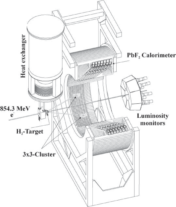
Figure 1: Set-up of the A4 experiment. The 854.3 MeV electron beam enters the 10 cm liquid hydrogen target cell made from thin aluminum from the left. Above the liquid hydrogen target the heat exchanger is located. The PbF₂ calorimeter consists of 1022 crystals and is shown as a sectional view with parts of it removed for better visibility. The 8 water Cherenkov luminosity monitors are placed at electron scattering angles of 4.4^∘ $<$ $\theta_{e}$ $<$ 10^∘ downstream the calorimeter.

The experimental asymmetry $A_{\mathrm{Exp}}$ is extracted from the number of counts of elastic scattered electrons $N^{\pm}$ for right ($+$) and left handed ($-$) electron beam helicity, respectively, normalized to the integrated effective target density $\rho^{\pm}$:

$$A_{\mathrm{Exp}} = \frac{(N^{+}/\rho^{+})-(N^{-}/\rho^{-})}{(N^{+}/\rho^{+})+(N^{-}/\rho^{-})}$$ (1)

$$= \frac{N^{+}-N^{-}}{N^{+}+N^{-}}+\frac{I^{+}-I^{-}}{I^{+}+I^{-}}-\frac{L^{+}-L^{-}}{L^{+}+L^{-}}+\mathcal{O}(10^{-12})$$ (2)

$$= A_{\mathrm{phys}}+A_{I}-A_{L},$$ (3)

where the effective target density $\rho^{\pm}$ of a fixed-target experiment is the luminosity $L^{\pm}$ divided by the beam current $I^{\pm}$. $A_{\mathrm{phys}}$ denotes the PV physics asymmetry in elastic electron proton scattering which is of order 10^-6. $A_{I}$ is a possible apparative asymmetry in the incoming beam current which is in the experiment of order $10^{-6}$. $A_{L}$ corresponds to a possible asymmetry in the luminosity signal also of order $10^{-6}$.

The A4 experiment measures very small (order 10^-6) PV cross section asymmetries. Accordingly, the following considerations have been taken into account for the design of the luminosity monitors:

• A measurement of the absolute luminosity is not necessary since any efficiency or calibration factor cancels in the ratio in Eq. 1, as long as it is exactly equal for both helicity states. This is accomplished by flipping the electron beam helicity at a rate (25 Hz) which is fast compared to most external fluctuation sources [6].

• The physical process which is used to measure the luminosity should have no (or very small) PV asymmetry. Possible processes contributing to the measured luminosity signal are elastic electron proton scattering at small scattering angles and elastic electron electron (Møller) scattering. We have optimized the response behavior of the luminosity monitor for the detection of Møller scattering.

• The accuracy in the PV asymmetry measurement should be dominated by the count rate accuracy (i.e. $\sqrt{N}$) and not by target density fluctuations, which may arise from temperature fluctuations or from boiling in the liquid hydrogen target caused by the heat deposition of the intense 20 $\mu$A electron beam in the hydrogen target. In order to accurately correct the measured asymmetry for target density fluctuations, we designed a monitor capable of measuring fluctuations with a relative accuracy on the level of $10^{-5}$ in 20 ms.

• The correct determination of false asymmetries arising from helicity correlated beam parameter fluctuations is necessary to measure the luminosity in order to disentangle beam current fluctuations from target density fluctuations as can be seen in Eq. 3.

• Due to the fact that in the A4 experiment counting of individually scattered particles is applied to a measurement of a parity violating asymmetry, effects of dead time in the counting electronics have to be considered. Systematic changes of the measured asymmetry can arise not only from differences in the integrated luminosity $L^{\pm}$ for positive ($+$) and negative ($-$) helicity, but also from fluctuations or differences of fluctuations in the luminosity which makes the simultaneous measurement of the square of the luminosity necessary.

2 Luminosity measurement

In a fixed target experiment the luminosity is given by the product of the beam current times the area density of scattering centers in the target. The luminosity of an experiment describes the flux density of the scattering reaction partners. The product of luminosity $L$ and cross section $\sigma$ results in an observed reaction rate $R=\sigma\cdot L$. A possible experimental method to determine the luminosity is the measurement of the event rate of a scattering reaction with a well-known cross section. The expected luminosity in the A4 experiment can be calculated from the flux of the beam particles $\phi_{e}$ [electrons/s] and the effective area target density $\hat{\rho}_{H_{2}}$ [atoms/cm²] by $L=\phi_{e}\cdot\hat{\rho}_{H_{2}}$. For a beam current of 20 $\mu$A and a target length of 10 cm the nominal luminosity in the A4 experiment is $L=5.3\cdot 10^{37}$s^-1 cm^-2.
Target density fluctuations, which are caused by boiling inside the hydrogen volume of the target and at the entrance and exit aluminum windows, can lead to large luminosity fluctuations compromising the statistical accuracy of the experiment. Since the A4 experiment does not use rastering of the 20 $\mu$A electron beam the avoidance of target boiling poses a delicate problem which is overcome by a highly turbulent flow of liquid hydrogen in the target cell and a wide electron beam profile in the hydrogen target cell [7].

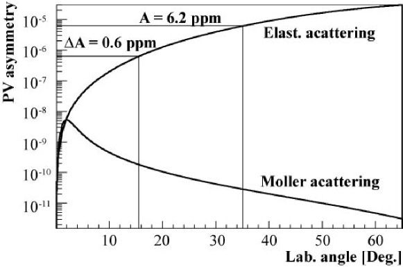
Figure 2: Parity violating asymmetries of Møller scattering and elastic scattering as a function of the electron scattering angle in the laboratory $\theta_{e}$. The water Cherenkov luminosity detector spans an interval in $\theta_{e}$ from $4.4^{\circ}<\theta_{e}<10^{\circ}$ and the PbF₂ calorimeter spans an interval from $30^{\circ}<\theta_{e}<40^{\circ}$.

Elastic as well as Møller scattering both exhibit a PV asymmetry. A PV asymmetry smaller than the statistical accuracy of the A4 experiment is required for the luminosity measurement in order to be able to correct for asymmetries of the luminosity with sufficient accuracy. The asymmetry of elastic and Møller scattering is shown in Fig. 2 as a function of the electron scattering angle $\theta_{e}$. For scattering angles $\theta_{e}\leq 15^{\circ}$ the asymmetry in the elastic scattering is smaller than the statistic accuracy of the A4 experiment ($\delta A_{0}=0.6\times 10^{-6}$). In the scattering angle range of the water Cherenkov luminosity detector of $4.4^{\circ}<\theta_{e}<10^{\circ}$ the elastic scattering has an asymmetry which is almost one order of magnitude less than the statistical accuracy of the A4 experiment. The asymmetry of the dominating Møller scattering is smaller by two orders of magnitude. At these angles the mean energy for Møller scattered electrons is 79 MeV while the mean energy for elastic scattered electrons is 848 MeV. This offers the possibility of tuning the energy response of the water Cherenkov luminosity detector to further suppress the unwanted elastic scattering process off the proton relative to Møller scattering.

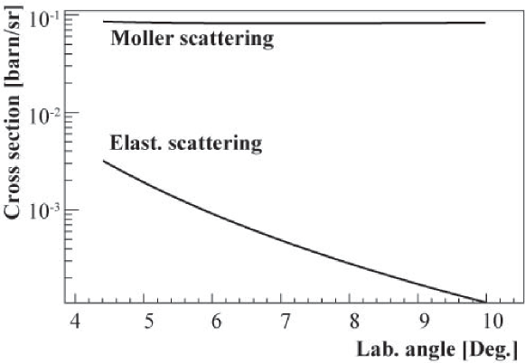
Figure 3: Differential cross section of Møller scattering and elastic scattering as a function of the electron scattering angle in the laboratory $\theta_{e}$. The water Cherenkov luminosity detector spans an interval in $\theta_{e}$ of $4.4^{\circ}<\theta_{e}<10^{\circ}$.

Elastic scattering on protons and Møller scattering dominate at small forward angles between $4.4^{\circ}<\theta_{e}<10^{\circ}$. As shown in Fig. 3, the probability for Møller scattering of beam electrons on electrons of the hydrogen target is a factor of 100 larger as compared to elastic electron proton scattering. The differential cross section for Møller scattering is almost constant over a wide range of scattering angle while the elastic cross section falls off as a function of the scattering angle.

An additional design requirement came from the fact that losses in counting rate due to dead time in the detector or the experiment electronics of the parity violation experiment have to be considered. The losses due to double hits affect the measurement in two ways: on one hand, pile-up reduces the measured counting rate, which can be compensated by an extension of the measuring time. On the other hand, pile-up losses due to background processes having a polarization dependent cross section can lead to a systematic change of the measured asymmetry. The first and most important step for reducing dead time effects was to find a detector material, that has a fast response behavior and, therefore, reduces dead time effects to the per cent level. The PbF₂ material employed in the A4 calorimeter is an intrinsically fast Cherenkov radiator with no slow scintillation components [8]. The PbF₂-detector electronics measures the energy within a 20 ns integration gate, which is the largest dead time in the system. It has a dead time-free digitization and a double hit (pile-up) identification for intervals of more than 5 ns [9]. Due to the non-linearity of the double hit rate losses, the fluctuations in the luminosity have to be measured separately for both polarization states to be able to correct for systematic changes in the experimental asymmetry. A detailed analysis of the effect of pile-up losses from a polarization dependent background process reveals a dependence on four quantities [6]:

1. The mean pile-up probability $\lambda$. Even with a perfect nonfluctuating beam where the polarization is equal for both helicity states, a finite pile-up probability leads to a systematic change of the measured asymmetry.

2. A difference of the pile-up probabilities $\Delta\lambda=\lambda^{+}-\lambda^{-}$ for the different helicity states of the beam arises if the luminosity for the two helicity states is different: $\langle\mathcal{L}^{+}\rangle\neq\langle\mathcal{L}^{-}\rangle$.

3. Fluctuations in the pile-up losses caused by fluctuations in the luminosity: $\eta(\frac{\delta\mathcal{L}^{+^{2}}}{\langle\mathcal{L}^{+}\rangle}+\frac{\delta\mathcal{L}^{-^{2}}}{\langle\mathcal{L}^{-}\rangle})$, where $\eta=2\tau\Sigma_{0}$, with $\tau$ the dead time (20 ns) and $\Sigma_{0}$ the cross section for elastic scattering. $\delta\mathcal{L}^{\pm}$ is the RMS of the luminosity. There is a systematic change of the measured asymmetry even if the integrated luminosities are equal, $\langle\mathcal{L}^{+}\rangle=\langle\mathcal{L}^{-}\rangle$, and even if the beam fluctuations are symmetric in helicity, $(\delta\mathcal{L}^{+})^{2}=(\delta\mathcal{L}^{-})^{2}$.

4. The difference of the pile-up losses caused by asymmetric luminosity fluctuations $\eta(\frac{\delta\mathcal{L}^{+^{2}}}{\langle\mathcal{L}^{+}\rangle}-\frac{\delta\mathcal{L}^{-^{2}}}{\langle\mathcal{L}^{-}\rangle})$. It causes a systematic change of the measured asymmetry if either the integrated luminosity or the RMS of the luminosity is different for the different helicity states, $(\delta\mathcal{L}^{+})^{2}\neq(\delta\mathcal{L}^{-})^{2}$.

We obtain the following formula for the systematic change of the measured asymmetry depending on the quantities defined above (please note that for the discussion of pile-up effects, we neglect for a moment other apparative asymmetries like A_I or A_L. If they are taken into account, we yield A_mathrmExp from A_Meas):

$$A_{\mathrm{Meas}}\!=\!\frac{\!-\!\Delta\lambda\!+\!(A_{u}\!+\!A_{0})2\lambda P\!+\!2A_{0}P\!-\!\eta\!\left(\!\frac{\delta\mathcal{L}^{+^{2}}}{\langle\mathcal{L}^{+}\rangle}\!-\!\frac{\delta\mathcal{L}^{-^{2}}}{\langle\mathcal{L}^{-}\rangle}\!\right)\!+\!\eta(A_{u}\!+\!A_{0})\!\left(\!\frac{\delta\mathcal{L}^{+^{2}}}{\langle\mathcal{L}^{+}\rangle}\!+\!\frac{\delta\mathcal{L}^{-^{2}}}{\langle\mathcal{L}^{-}\rangle}\!\right)\!P}{2\!-\!2\lambda\!-\!(A_{u}\!+\!A_{0})\Delta\lambda P\!-\!\eta\!\left(\!\frac{\delta\mathcal{L}^{+^{2}}}{\langle\mathcal{L}^{+}\rangle}\!+\!\frac{\delta\mathcal{L}^{-^{2}}}{\langle\mathcal{L}^{-}\rangle}\!\right)\!-\!\eta(A_{u}\!+\!A_{0})\!\left(\!\frac{\delta\mathcal{L}^{+^{2}}}{\langle\mathcal{L}^{+}\rangle}\!-\!\frac{\delta\mathcal{L}^{-^{2}}}{\langle\mathcal{L}^{-}\rangle}\!\right)\!P}$$

(4)

Even for very symmetric beam conditions with equal integrated luminosities $\langle\mathcal{L}^{+}\rangle=\langle\mathcal{L}^{-}\rangle$, equal luminosity fluctuations $\delta\mathcal{L}^{+^{2}}=\delta\mathcal{L}^{-^{2}}$, and equal polarization for both helicity states $P^{+}=P^{-}$, double hit losses from a polarization dependent background process with asymmetry $A_{u}$ lead to a systematic change of the measured asymmetry $A_{\mathrm{Meas}}$ as compared to the physics asymmetry $A_{0}$. In this case Eq. 4 may be simplified to:

$$A_{\mathrm{Meas}}=\frac{A_{0}P-(A_{u}+A_{0})\lambda P}{1-\lambda}$$ (5)

Due to rate losses by pile-up, as just discussed, an important design requirement was the measurement of the variance (RMS) of the luminosity signal, in addition to the integrated luminosity $\langle L\rangle$, by measuring the second moment of the luminosity, $\langle L^{2}\rangle$. From this, the variance can be extracted: $\langle(\langle L\rangle-L)^{2}\rangle=\delta L^{2}=\langle L^{2}\rangle-\langle L\rangle^{2}$. The required accuracy of the luminosity measurement for an experimental error of $\delta$A_Exp/A_Exp = 1 % in a measurement gate of 20 ms is:

$$\frac{\Delta L}{L}=3\times 10^{-5},\quad\sqrt{\frac{\delta L^{2}}{\langle L\rangle^{2}}}=5\times 10^{-3}.$$ (6)

This ensures that the experimental asymmetry can be corrected to pile-up effects caused by luminosity fluctuations with an accuracy of better than 1%. On account of the short dead time of the PbF₂ detectors and the fast readout electronics, the losses due to double hits in the calorimeter are 1.7% at 20 $\mu$A beam current and a luminosity of 5 $\times$ 10³⁷ cm^-2s^-1.

False asymmetries may also arise from noise signals correlated with the power line frequency (50 Hz) and higher harmonics as well as beam fluctuations or systematic effects correlated with the helicity flip. For this reason, the measurement of the luminosity is synchronized to the power line frequency, i.e. the integration gate length is the inverse of the current power line frequency ($\approx$20 ms). The length of the integration gate is synchronized by a phase locked loop (PLL) to the line frequency. For normalization purposes the gate length was measured for each helicity state. Between two 20 ms integration gates a 80 $\mu$s time window for the change of the electron beam helicity by changing the high voltage at the Pockels cell [10] is needed. The 80 $\mu$s time window guarantees that the Pockels cell voltage has reached a stable condition. However, it introduces a phase shift of the integration gate with respect to the line frequency. The phase shift is (80/2080)2$\pi$ and after 25 gate pulses the phase difference is zero again.

We use two different patterns of helicity for four consecutive integration gates: ($+--+$) and its complement ($-++-$). Both have the same number of $+$ and $-$ helicity states. The patterns are chosen randomly by a bit shift register. Since a helicity flip corresponds to a fast high voltage change at the Pockels cell which might induce electromagnetic pick-up signals the patterns chosen guarantee that the helicity flip is equiprobable and that a correlation of the asymmetry with the polarization sequence is avoided.

3 Design and construction of the luminosity monitor

The design of the luminosity monitors is based on a water Cherenkov detector system read out by photomultiplier tubes. Eight modules are used which cover an azimuthal electron scattering angle $\phi_{e}$ of 2$\pi$, while the polar electron scattering angle range is $4.4^{\circ}<\theta_{e}<10^{\circ}$. The high event rate of 5.5 GHz per module requires an integrating measurement of the anode current of the photomultiplier tubes.

With the program package GEANT 3.21 of the CERN software library the response behavior of the luminosity was simulated and optimized. As already discussed, the energy of Møller electrons is an order of magnitude lower than that of elastic scattered electrons. The simulations were done for a stainless steel tank filled with demineralized water and a photomultiplier tube attached to a quartz-window of the steel tank. The optical transmission of water was taken into account as well as the quantum efficiency of the photocathode. In the simulations we selected rhodium mirrors on the inner faces of the luminosity monitor. Despite its high price, rhodium was chosen due to its reflectivity and good resistance to ionized water. The energy loss of electrons in the water volume, the production of Cherenkov light, and its collection on the photocathode of the photomultiplier tube was simulated. Electrons with appropriate energies were injected directly into a module of the luminosity monitor. Three parameters turned out to be the most important for the response behavior of the detector:

• The first variable is the mean number of Cherenkov photo-electrons from Møller electrons $N_{\mathrm{M{\o}ller}}^{Photons}$ which determines the statistical accuracy of the luminosity measurement. It is given by the development of the electromagnetic shower induced by a Møller electron as it evolves in the water volume and also by the production of Cherenkov photons from charged particle tracks.

• The fluctuation of $N_{\mathrm{M{\o}ller}}^{Photons}$ has two contributions: the usual $\sqrt{N}$ behavior and an additional fluctuation coming from the electromagnetic shower fluctuations. In order to minimize the shower fluctuations we optimized the ratio $E^{\mathrm{M{\o}ller}}/\sigma_{E}^{\mathrm{M{\o}ller}}$ of the mean deposited energy $E^{\mathrm{M{\o}ller}}$ of Møller electrons in the detector volume and the RMS of the energy deposit of Møller electrons $\sigma_{E}^{\mathrm{M{\o}ller}}$.

• In addition, we wanted to suppress the response of the detector to elastic scattered electrons by maximizing the ratio of the mean deposited energy of the Møller electrons over that of elastic scattered electrons $E^{\mathrm{M{\o}ller}}/E^{\mathrm{elastic}}$.

For determining the design parameters of luminosity monitors we have simulated different lengths of the detector modules in search of the maximum of the product of the three factors discussed above:

$$\mathrm{FOM} = N_{\mathrm{M{\o}ller}}^{Photons}\frac{E^{\mathrm{M{\o}ller}}}{\sigma_{E}^{\mathrm{M{\o}ller}}}\frac{E^{\mathrm{M{\o}ller}}}{E^{\mathrm{elastic}}}$$ (7)

The figure of merit as extracted from the full GEANT simulation of the water Cherenkov luminosity detector is shown in Fig. 4. The optimum detector length can be read off the figure to be 20 cm.

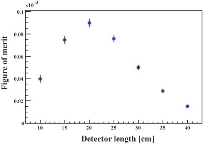
Figure 4: Figure of merit (as defined in Eq. LABEL:eq:fomlumi) as a function of the length of the water volume determined by GEANT simulations (see text).

Due to the ring geometry the monitor modules have the shape of a frustum of pyramid with a trapezoidal base. The depth of a module in beam direction is 20 cm. The readout of Cherenkov light is done with quartz window photomultiplier tubes which are separated by quartz windows (HOQ310, Heraeus Quartzglas, Hanau, Germany) from the water volume and are placed in a light-tight aluminum housing (Fig. 5 top). The luminosity monitors are attached to the downstream end of the A4 scattering chamber. The flange of the scattering chamber was milled down to 5 mm thickness in the angular range from $4^{\circ}<\theta_{e}<10^{\circ}$ in order to minimize the energy loss of scattered electrons before entering the luminosity monitors.

Figure 5: Top: Photograph of two out of eight neighboring luminosity monitors with the photomultiplier tubes attached. Bottom: Detailed CAD drawing of a luminosity monitor in side view and from the rear face.

Due to the high radiation dose during the experiment of $>1$ Mrad per 1000 h it is necessary to use radiation resistant materials. The photomultiplier tubes are equipped with quartz windows. In order to avoid the production of radicals in the water volume distilled water is used. The detector modules had to be built with as little material as possible in order to minimize backscattering from the luminosity monitors into the PbF₂ calorimeter. The material of the support structure of the monitors had been minimized, too. Each of the eight modules consists of a water tank with 1 mm thick steel walls. Two of the modules are shown in Fig. 5. The detector housing is manufactured of high-grade stainless steel in order to avoid corrosion by the water. The photomultiplier tube, attached to the rear face of the water tank, is housed in a light tight cylinder made of aluminum. In the experiment, we did not use rhodium mirrors at the inner faces. The voltage divider of the photomultiplier tube is outside of this cylinder to avoid overheating. The two flanges on the rear face of the water tank would allow the circulation of the water, if necessary. During our experiment we found that this was not necessary. Due to the activation during the experiment all parts of the detector are fixed by screws so that in case of a defect a module can be dismounted within a very short time. Figure 5 (bottom) shows a drawing with details of the detector. Table 1 summarizes the specifications of the luminosity monitors.

Table 1: Specifications of the water Cherenkov luminosity detectors:

water Cherenkov detector optimized for Møller (FOM)
8 modules	$4.4^{\circ}<\theta_{e}<10^{\circ}$
	$0^{\circ}<\phi_{e}<360^{\circ}$
	$\Delta\phi_{e}=45^{\circ}$
solid angle per module	9.97 msr
rates per module:	0.3 GHz (elastic)
	43.8 GHz (Møller)
	44.1 GHz total event rate
readout	integrating anode current
accuracy per module:	$\Delta\mathcal{L}/\mathcal{L}=3.4\cdot 10^{-5}$ (in 20 ms)
radiation dose	$\approx$ 1.4 Mrad per 1000 h

We use Philips XP3468B photomultiplier tubes with 8 dynodes where we have bypassed the last three dynodes. This photomultiplier tube has a diameter of 76 mm and a length of 164 mm. The entrance window has a diameter of 76 mm, the sensitive surface of the photocathode has a diameter of 68 mm. This tube size was selected for a good coverage of the rear face of the luminosity monitors. A transparent coupling in the whole spectral region must be achieved at the connection between the detector window and the photomultiplier tube, for which the radiation resistant silicone rubber Elastosil RT 601 is used. The rate per module amounts to $44.1\cdot 10^{9}$ Hz. One Møller scattered electron produces approximately 170 photons. Per 20 ms integration gate, $7.5\cdot 10^{12}$ photons are produced. With a quantum efficiency of the photocathode of about 20% this corresponds to $1.5\cdot 10^{12}$ photoelectrons. The maximum input current of the electronics amounts to 100 $\mu$A equivalent to $6.24\cdot 10^{14}$ electrons per second. Accordingly, the amplification factor of the photomultiplier tube has to be limited to $5\cdot 10^{3}$ which was realized by using only 5 dynodes.

4 Electronics and Readout

The A4 experiment luminosity electronics was developed and built in-house. For the eight signals from the luminosity monitors, the raw signal and the squared signal have to be integrated and digitized. There are more signals from beam parameter monitors like horizontal and vertical position monitors at different places in the accelerator, electron beam current monitor, and electron energy monitor in the accelerator etc. These signals are integrated over 20 ms, digitized and histogramming by modules of this part of the electronics. The A4 PV-experiment is controlled by a gate generator which delivers a gate signal to the calorimeter electronics and monitoring electronics.

An electronics unit for one water Cherenkov luminosity monitor consists of two modules (module A and module B in Fig. 6). Module A contains two internal channels (LIN and QUAD in Fig. 6). Channel LIN contains an integrator circuit for the linear luminosity signal and a 16 bit analog-to-digital (ADC). Channel QUAD has, in addition, a squaring device in front of the integration circuit. The squaring device is an analogue multiplication device. The accuracy of the linearity of the electronic multipliers amounts to $\approx 5\cdot 10^{-3}$. The integral and differential linearity of the 16 bit ADC is less than 1 LSB (least significant bit). The module A with the integrator (LIN) and squaring device (QUAD) permits a measurement of the first and second moment of the luminosity. The module B contains the histogramming modules. Data are transferred by an optically insulated serial interface to the histogramming units. The histogramming module has 4 MB RAM per channel (16 bit data depth, 21 bit addresses) which can store separated histograms for each polarization state. The integration gate of 20 ms can be divided, if necessary, into 16 time slices, so that the structure of the luminosity within a 20 ms gate can be examined. One time slice has a length of 1.25 ms.

The measurement of small (of order $10^{-6}$) asymmetries requires special care in isolating the integrator, squaring device, and ADC - all housed in module A of Fig. 6 - from outside noise or electromagnetic pickup. The module A and B are galvanically separated so that the digital signals from the histogramming module B can not induce noise in module A. The polarization information (polarization bit, $P$-bit) is electronically encoded in different voltage and current levels which could cause small changes of the current and voltage distribution of the electronic circuit. This results in different current distributions on the ground plane of the electronics circuit and different potential differences for the two helicity states. A careful design of the ground plane in the electronics circuit of module A is necessary in order to avoid small shifts of the zero Volt ground level at the input of the integrator, squaring device, or ADC which would result in false asymmetries of the measured signal charges. Such cross talk of the P-bit to the luminosity measurement is carefully avoided.

The histogramming module B contains a programmable logic unit which allows to operate the module in different ways:

• If operated as a pure histogramming module, the output of the ADC is - depending on the value of the $P$-bit - interpreted as an address and the memory content of that address cell is increased by one. After the run measurement time one can readout two histograms (one for each polarization state) directly via VME-bus from the memory of the histogramming module. Correlation between different luminosity monitor modules is lost that way but has the advantage that no additional data treatment is necessary to create histograms out of the data.

• For diagnostics reasons one can operate the module in a “timing” mode, where each 20 ms integration the ADC-output is stored directly in memory. This mode stores all signals as a function of time up to 30 minutes and gives the opportunity to correlate all signals with each other. The polarization bit is stored with each ADC value.

The timing control of the integrators, ADCs and the histogramming units is synchronized by one additional module (“Histo Master” in Fig. 6) giving control signals to all the modules.

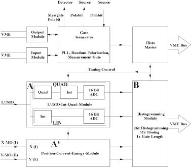
Figure 6: Scheme of the A4 monitoring electronics.

The noise of the electronics and any false asymmetry induced by the electronics was measured to be well below the desired accuracy of $3\cdot 10^{-5}$ and can, therefore, be safely neglected.

Additional beam monitor signals from the accelerator are integrated and digitized by a module similar to module A in Fig. 6. This additional module (Module A’ in Fig. 6) has two individual input channels with a linear integrator and ADC each. In total, one has 8 Luminosity monitor signals (LIN and QUAD in 8 modules from type A) and 10 more signals from the accelerator (readout by 5 modules from type A’). The data from the modules of type A and A’ are stored twice in two modules from type B in order to create redundancy and detect changes of individual hardware memory bits by ionizing radiation.

A further VME-bus module measures the length of the integration gate for each polarization state by a 35 bit counter and histograms it. An external 20 MHz quartz (generator) serves as time base. The measured asymmetry in the integration gate length, which serves as the integration and counting window for the whole parity experiment, is less than 10${}^{-}9$. Thus, a high absolute accuracy for the measurement of small (order 10^-6) asymmetries in the luminosity and other accelerator beam parameter signals was achieved.

5 Performance and Measurements

The performance and accuracy of the luminosity monitors was investigated in several experiments. With the luminosity monitors, the target density fluctuations of the liquid hydrogen target were studied.
From a simultaneous measurement of the beam intensity and the luminosity, target density fluctuations can be detected and analyzed. The result of such a study is shown in Fig.7, for different conditions of the electron beam size and position. In Fig. 7 the luminosity monitor (LUMO) signal and the signal of a beam current monitor (PIMO) are shown as a function of time. The PIMO is a microwave cavity with high Q-value which can be adjusted to measure either the phase (P) or the current (I) of the electron beam. For Fig. 7 the PIMO has been adjusted to measure the electron beam current. The top plot shows a signal of a single module as a function of time sampled every 20 ms, where the target has been operated in such a way so that target density fluctuations from boiling dominate. Boiling causes a fluctuation in the luminosity signals of $\pm$2.5%. For the middle figure, the diameter of the electron beam and the cooling performance of the hydrogen target were optimized and the beam had been 1 mm off axis. The fluctuations of the measured luminosity was reduced to $\pm$0.5% which can be identified as beam current fluctuations comparing them to the independent beam current signal in the bottom plot.

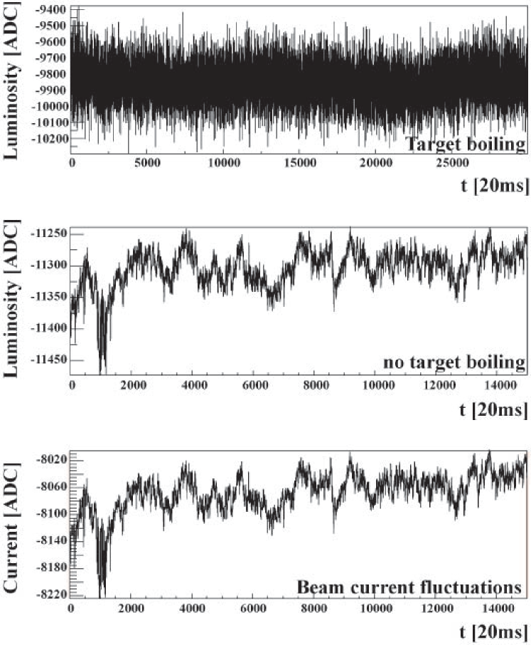
Figure 7: Example of target density and beam current fluctuations.

The correlation of the signals of two luminosity monitors allows us to separate intrinsic detector fluctuations like uncorrelated noise from external fluctuations in the luminosity signal caused by beam or target density fluctuations. The latter are correlated for two neighboring modules. For the determination of the uncorrelated noise, which limits the sensitivity, two neighboring luminosity monitors were combined. For two adjacent neighbors helicity correlated differences in position and angle are small. In Fig. 8, the averaged signal of luminosity monitor #5 is plotted versus the averaged signal of luminosity monitor #6. Both signals are strongly linearly correlated. We conclude that the observed signal fluctuations are caused by target density and beam fluctuations. For the graph in Fig. 8 (bottom) the residual of the non-averaged luminosity data of the same monitor and the straight line fit was calculated and sorted into a histogram. The RMS width of this distribution divided by $\sqrt{2}$ gives the experimental accuracy of a single luminosity measurement in 20 ms, $\delta L_{20ms}$. The RMS width divided by $\sqrt{N}\sqrt{2}$ gives the accuracy for our data taking running time of 5 minutes, $\delta L_{5min}$. For the data in Fig. 8, the mean luminosity signal corresponds to $(9862.4\pm 0.006)$ ADC channels. The relative accuracy results $(\delta L/L)_{5min}=6.1\cdot 10^{-7}$ in 5 minutes and $(\delta L/L)_{20ms}=7.5\cdot 10^{-5}$ in 20 ms. In comparison with the simulated accuracy of $(\Delta L/L)=3\times 10^{-5}$ it is worsened by a factor 2-3. This can be explained by the fact that the luminosity monitors are used without rhodium mirrors with correspondingly less light reaching the photocathode of the photomultiplier tube. Tests have shown that mirrors improve the accuracy by a factor 3-5. Thus, we can conclude that the simulations and the experimental results from the real luminosity monitors are in good agreement.

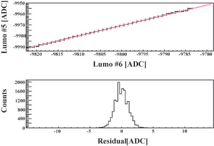
Figure 8: Determination of the accuracy of the luminosity monitors.

A correction was applied for the non-linearity of the luminosity monitor photomultiplier tubes. This was measured and verified separately by varying the beam current from 0 to 23 $\mu$A. A false asymmetry results from non-linearities in the response behavior of the luminosity system. The nonlinearity has to be measured and the data have to be corrected, accordingly. Without this correction the false asymmetry would be about $5\times 10^{-9}$ per percent nonlinearity (see Fig. 9) at a beam current asymmetry of 10${-6}$. A non-linearity of 1 % in the response behavior of the luminosity system causes a false asymmetry of $5\cdot 10^{-9}$. Fig. 9 shows the signal of a luminosity monitor as a function of a beam current variation from 0 to 23 $\mu A$ as measured with the linear beam current monitor PIMO. Nonlinearities at high beam currents are readily seen in the upper plot. The lower part shows the local steepness by deviation from zero. The steepness varies as much as 8 % from 0 $\mu$A to 20 $\mu$A. The non-linear deviation from the straight line fit is 8.0% at the operating point of the A4 experiment of 20 $\mu$A (here the PIMO signal is $\approx$ 8700 ADC channels). If not corrected this would cause a false asymmetry of $-4\cdot 10^{-8}$ for a beam current asymmetry of $1\cdot 10^{-6}$. Actual beam current asymmetries vary between $1\cdot 10^{-8}$ and $1\cdot 10^{-5}$.

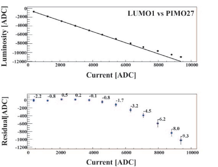
Figure 9: Top: Signal of luminosity monitor as a function of the beam current monitor signal. Bottom: The points give the absolute difference of the measured data from the the straight line fit. The numbers give the relative deviation in percent.

We corrected the non-linearities in the luminosity signals with the measured counting rates of the PbF₂ calorimeter since both detector systems see the same luminosity. This detector system was shown to be linear after correction for pile-up losses even for high beam currents. The non-linearity of the luminosity signals has been corrected without correlation to helicity, i.e. the counting rates of both helicities of the luminosity monitors and the counting rates of the PbF₂ calorimeter (in Fig. 10 called MEDUSA) were added. Due to the small current asymmetry within the range of $10^{-6}$ to $10^{-5}$ the correction factor of the non-linearity of the luminosity monitors is not helicity dependent. The interpolation of the non-linearity of the luminosity monitors can be very well approximated by a $\tanh$-function. Fig. 10 shows the implementation of the non-linearity correction. The figure shows, on the one hand, the luminosity raw data on the tanh-curve and, on the other hand, the corrected luminosity data on the straight line fit which describes the linearized and corrected data.

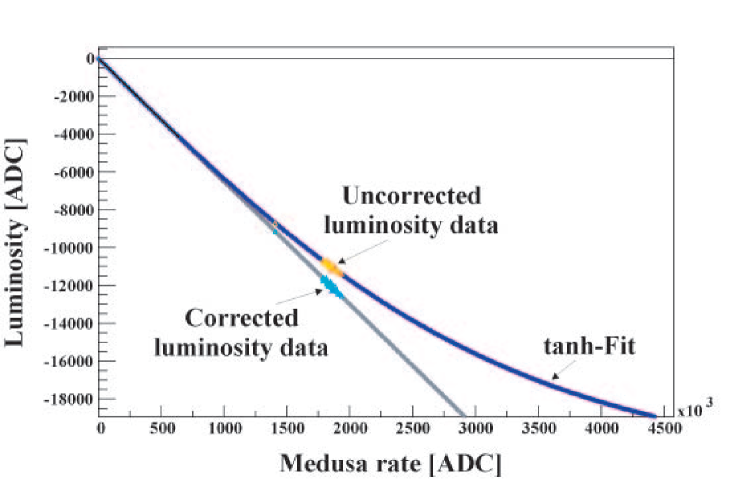
Figure 10: Correction of LUMO-Data via hyperbolic tangent.

Another important point is the investigation of target density fluctuations caused by heating due to the energy deposition of the electron beam in the hydrogen. The scheme of the target cell is shown in Fig. 11. The 10 cm liquid hydrogen target provides a luminosity of $L=5\cdot 10^{37}$ cm^-2s^-1 at 20 $\mu$A electron beam current. This corresponds to about 100 W of heat absorbed in the liquid hydrogen and in the two windows cooled by the hydrogen. The target has a closed loop circulating system cooled by a helium refrigerator. Thus, the temperature of the hydrogen entering the target cell is just above the hydrogen freezing point, much below the boiling temperature (deeply subcooled hydrogen). The design of the liquid hydrogen loop and the target cell were optimized to obtain a high degree of turbulence with a Reynolds number of $R>2\times 10^{5}$ in the target cell in order to increase the effective heat transfer. The heat exchange is intensified by transverse turbulent mixing which causes a faster mass exchange across the hydrogen stream. This approach removes the heat deposit by the electron beam which is concentrated in a small range around the beam axis and which can cause fast luminosity fluctuations from hydrogen density variations or boiling of the liquid at the windows. This new technique allowed us, for the first time, to avoid a fast modulation of the beam position (rastering) of the intense CW 20 $\mu$A electron beam. It permitted us to stabilize the beam position on the target cell with less than 10^-3 relative target density fluctuations arising from boiling. The cooling system supports a high flow rate of liquid hydrogen and up to 250 W heat load of beam energy deposition in the target.

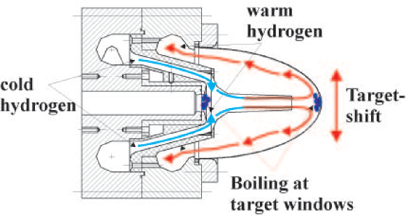
Figure 11: Scheme of the target cell.

We investigated the effect of beam diameter variations on target boiling and luminosity fluctuations. In this context, “fluctuation” refers to the point to point difference of the measured luminosity signals for two neighboring 20 ms integration gates. The fluctuations of the luminosity signal were measured as a function of the electron beam cross section from 5$\times$ 10⁵ $\mu$m² up to 3$\times$ 10⁶ $\mu$m² and the impact position of the electron beam at the target. The results of the measurements are presented in Fig. 12. One recognizes that an enlargement of the beam diameter (runs 3000-6500) causes a decrease of the fluctuations by a factor 4-5. The measured fluctuations correlate with increasing beam diameter as the heat deposition in the target is distributed on a larger area and the density of deposited energy is smaller.

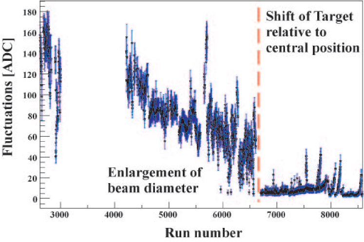
Figure 12: Investigations of target density fluctuations.

Additional boiling at the entrance and exit windows of aluminum has a large influence on the observed luminosity fluctuations. The calculated specific heat flow from the windows into the liquid hydrogen exceeds the critical point for boiling on the surface, even for an enlarged beam spot. Therefore, boiling at the windows does take place. A detailed analysis that includes the aluminum heat conductivity shows that this process does not depend very much neither on the beam size nor on the wall thickness. One way to reduce a bubble content in the beam region is the increase of the mass flow tangentially to the window surface. That is achieved in the present axially symmetric construction of the target cell by shifting the target axis relative to the axis of the beam. For a systematic investigation of the boiling at the target windows, the target position was varied in the range of 5 mm in vertical direction (from 2 mm below to 3 mm above the beam position) and the fluctuations were measured with the luminosity monitors. It was found, that shifting the target position by 1 mm out of the center reduces the fluctuations by a factor 4 (The result can be seen in Fig. 12, runs 6700-8500). If the electron beam hits accurately the center of the target nose the heat cannot be removed as efficiently as in a position 1 mm above or below the center of symmetry. We found a reduction in the width of the asymmetry distribution around an order of magnitude after the reduction of the target boiling. Eliminating the target boiling controlled by the luminosity monitor plays an essential role in the experiment. The measured asymmetry caused essentially by beam current asymmetries reduces from $(-4.61\pm 1.02)$ ppm to $(-0.89\pm 0.31)$ ppm. The error of the measured asymmetry reduces from of 1.02 ppm to 0.31 ppm.

6 Summary

A luminosity monitor system was developed to correct the A4 asymmetry data to target density fluctuations. The system determines the luminosity and the RMS of the luminosity in a 20 ms integration gate. The system was studied and optimized in simulations. The radiation-hard luminosity monitor measures in pulse integrating mode at very small forward scattering angles and achieves a relative accuracy of $\delta L/L=7.5\cdot 10^{-5}\pm 4\cdot 10^{-7}$ in 20 ms. The use of such a monitor system not only allows us to learn about the state of the hydrogen target but also enables us to correct the measured rates to the actual (square) luminosity. This enhances the accuracy of the parity violation measurement by a factor of 3.

7 Acknowledgements

This work was supported by the Deutsche Forschungsgemeinschaft in the framework of the SFB 201 and the SPP 1034. The development of this electronics took place in co-operation with the electronics workshop of the Institut für Kernphysik Mainz in collaboration with R. Böhm, G. Hacker, J. Reinemann and H. Streit.

References

- [1] F. E. Maas et al., Measurement of strange quark contributions to the nucleon’s form factors at =0.230 (gev/c)2, Phys. Rev. Lett. 93 (2004) 022002.
- [2] F. E. Maas et al., Measurement of the transverse beam spin asymmetry in elastic electron proton scattering and the inelastic contribution to the imaginary part of the two-photon exchange amplitude, Phys. Rev. Lett. 94 (2005) 082001.
- [3] F. E. Maas et al., Evidence for strange-quark contributions to the nucleon’s form factors at =0.108(gev/), Phys. Rev. Lett. (2005) in print.
- [4] F. E. Maas et al., Parity violating electron scattering at the mami facility in mainz: The strangeness contribution to the form-factors of the nucleon, Eur. Phys. J. A 17 (2003) 339.
- [5] F. E. Maas et al., Proc. of the ICATPP-7, World Scientific, 2002, p. 758.
- [6] T. Hammel, Luminosit zur messung der paritätsverletzung in der elastischen elektronenstreuung, Ph.D. thesis, Mainz University (2004).
- [7] I. Altarev, et al., A high power liquid hydrogen target for the mainz a4 parity violation experiment., in preparation to be submitted to Nucl. Instr. and Meth. A.
- [8] P. Achenbach et al., measurements and simulations of cerenkov light in lead fluoride crystals, Nucl. Instrum. Meth. A 465 (2001) 318.
- [9] S. Köbis et al., The analog trigger processor for the new parity violation experiment at mami, Nuclear Physics B 61B (1998) 625.
- [10] K. Aulenbacher et al., The mami source of polarised electrons, Nucl.Ins.Meth.A 391 (1997) 498.