Low-Energy Deuteron Polarimeter

Abstract

We built a Low Energy Deuteron Polarimeter (LDP) which measures the spin-polarization of deuteron beams in the energy range of 25 to 80 keV. The LDP works by measuring azimuthal asymmetries in the D($\vec{d},n$)³He reaction at $\theta_{lab}=90^{\circ}$ and comparing them to analyzing powers. We built this polarimeter for two reasons. Firstly, to cross-check other polarimeters at KVI (LSP and IBP). Secondly to test the LDP itself. We were able to use the LDP as a vector polarimeter, but not as a tensor polarimeter because of an uncertain tensor analyzing power calibration.

Figure 1: Cartoon depicting polarization. The top panel represents a polarized beam, where spins are aligned. The bottom panel represents an unpolarized beam, where spins are randomly aligned.

1 Introduction

Most people know that light can be polarized. This means that light oscillates in a preferred plane. All nuclear physicists know that ‘particle beams’ can be ‘spin-polarized’. This means that particles making up a beam have their spins aligned in a preferred direction as is illustrated in Fig. 1 (page 2).

The linear polarization of light can be determined, quite easily, with a polarizing filter. An analogous device, called the Stern-Gerlach filter, can determine the polarization of beams of neutral particles by splitting the beam according to its spin content. Here the degree of polarization would be the excess in quantity of one spin-state over another spin-state.

Most beams in nuclear physics are made of charged particles such as electrons, protons, nuclei, or as in this experiment, deuterons. A deuteron is an atomic nucleus consisting of a proton and a neutron. Only beams of charged particles can be manipulated (accelerated, steered, focused ) by the electric and magnetic fields of the machinery in accelerator facilities, such as in KVI. Neutral beams are weakly affected by electric and magnetic fields. Measuring the polarization of beams of charged particles, as opposed to beams of neutral particles, is more difficult because polarization filters such as the polaroid or the Stern-Gerlach filters do not exist for charged particles. Mott and Pauli  [1, 2], therefore many textbooks in Quantum Mechanics, claim that a spin filter for charged particles is theoretically impossible. Yet it was recently claimed [3] that such a device is possible under particular conditions. Until such a device is built, or proved unfeasible, the polarization of charged particle beams is determined by scattering experiments. Measuring polarization may seem to be a trivial measurement. But since it is a fully-fledged scattering experiment it involves beam, target, detectors, and electronics, therefore takes months to accomplish.

1.1 Nomenclature

Particle beam polarimetry borrowed nomenclature from optical polarimetry. This is not surprising in view of the similarities between spin polarization and optical polarization.

Physics textbooks often describe an experiment with two polarizing filters at an angle to each other; the first filter is called the ‘polarizer’ and the second is called ‘analyzer’. The wording is such because the first filter can polarize (normally unpolarized) light, while the second filter can analyze the strength and direction of the polarization. In nuclear physics polarimetry, a reaction of the type A($b,\vec{c}$)D is called a ‘polarization experiment’. The vector stands for a polarized specie. In this reaction an unpolarized beam $b$, creates a polarized ejectile $\vec{c}$. A reaction of the type A($\vec{b},c$)D is called ‘analyzing power experiment’ because a beam, $\vec{b}$, with non-zero polarization creates an asymmetry in the ejectile’s distribution. The word ‘analyzer’ of optics became ’analyzing power’ in nuclear physics. In optics any analyzer is as good as the next one, while in nuclear physics different reactions have different analyzing efficiencies, hence the word analyzing power.

1.2 Why Make Polarized Beams?

Polarized beams or targets are used in nuclear physics to extract observables such as analyzing powers and spin-transfer coefficients. These measured observables can be compared to predictions of theoretical models to study, for example, the three-body force [4, 5], or the spin-terms of the nucleon-nucleon potential.

One application of polarized beams lies in the possibility [6, 7] of using polarized deuteron beams to control the reaction rates in fusion reactors and to reduce the amount of unwanted neutrons.

1.3 Our Motivation

Our motivation to measure polarization stems from the fact that two polarimeters at different beam energies measure different polarizations. One polarimeter, called the In-Beam Polarimeter (IBP), measures less polarization than another polarimeter, the Lamb-Shift Polarimeter (LSP). By building a third polarimeter, this Low-Energy Deuteron Polarimeter (LDP), and comparing its results with the other two polarimeters, we wish to determine whether one of the polarimeter is inaccurate or whether the polarization changes between polarimeters. For beams of polarized protons, the LSP routinely measures polarization between 80-90 $\pm$ 1% (of the theoretical maximum), while the IBP measures 70-75 $\pm$ 4%. Since laboratories, other than KVI, are not able to produce polarizations reaching 90%, a healthy skepticism exists in the LSP’s reading of 90%. This new polarimeter, the LDP, which measures essentially the same beam as the LSP (in terms of beam energy, current and location), can determine whether the LSP systematically overestimates the polarization or not. If the LSP and LDP agree on the polarization, one can conclude that there are polarization transformations. While if the LDP agrees with the IBP, we conclude that the LSP overestimates polarization due to some unknown systematic uncertainty.

Another motivation is that, a deuteron polarimeter based on the D($d,n$)³He reaction has not been published before. Building the LDP is a feasibility test for a new polarimeter. The standard reactions, for deuteron polarimetry at these energies, are ³H($d,n$)⁴He and D($d,p$)³H. The advantage of our reaction over these two is, respectively, that it does not involve handling of tritium, and does need to have detectors inside the scattering chamber.

1.4 Concept Behind Polarimetry

By impinging a beam on a target and observing the distribution of scattered particles in space, one can deduce the polarization of the beam.

An unpolarized beam scatters particles with an isotropic (azimuthal) distribution, while a polarized beam scatters particles with a non-isotropic (azimuthal) distribution. The latter case is illustrated in Fig. 2.

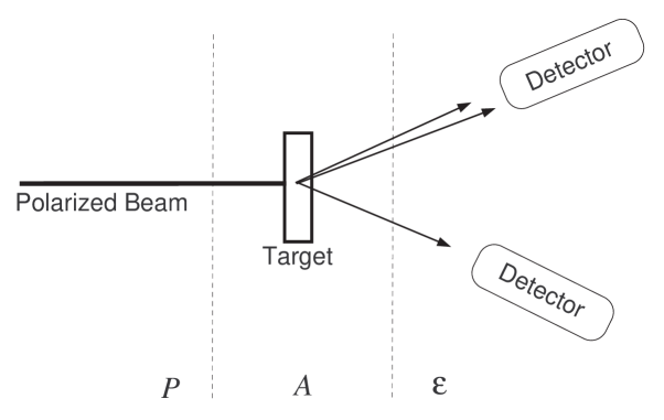
Figure 2: A scattering experiment. A polarized beam impinges on a target. The ejectiles scatter preferentially in some direction. Two detectors measure an asymmetry in the number of ejectiles. The figure also shows to which parts of the experiment the quantities $P$ (polarization), $A$ (analyzing power), and $\epsilon$ (asymmetry) are associated with.

The degree of non-isotropy in scattering is quantified by the ‘asymmetry’ that detectors measure, and is proportional to the beam polarization with a proportionality constant given by the analyzing power. Mathematically,

$$\epsilon=PA.$$

This equation describes how polarimeters based on scattering, such as the LDP and IBP, work. In our experiment $P$ is the quantity which we solve for in terms of $\epsilon$ and $A$. $\epsilon$ is measured experimentally by the detectors. $A$ is a constant that can be calculated or measured by other experiments.

2 Theoretical Background

2.1 Nuclear Potential

The nuclear potential is not yet fully understood, and is still a subject of research and lamentation. An illustrative, but incomplete, form of a two-nucleon nuclear potential is

$$V=V_{0}(r)+V_{s}(r)\,\vec{s_{1}}\cdot\vec{s_{2}}+V_{SL}(r)\,\vec{S}\cdot\vec{L}\\ +V_{T}(r)\,\ \Big{(}\frac{3}{r^{2}}(\vec{s_{1}}\cdot\vec{r})(\vec{s_{2}}\cdot\vec{r})-\vec{s_{1}}\cdot\vec{s_{2}}\Big{)}+\underbrace{\ldots}_{?}$$ (1)

Terms on the right side of the above equation are called central, spin-spin, spin-orbit, and tensor. The central term depends only on the distance separating the two nucleons. Another example of a central potential is gravitational attraction. The spin-spin term, $\vec{s_{1}}\cdot\vec{s_{2}}$, stems from the magnetic interaction of the spins of the two nucleons. The spin-orbit term, $\vec{S}\cdot\vec{L}$, stems from the interaction between the total spin of both nucleons and the angular momentum defined by their relative motion. An example of a spin-orbit interaction is the ‘fine structure’ in atomic physics; where the degeneracy for states of equal $L$ is lifted. An analogy of a tensor behavior is the interaction of two bar magnets. Two bar magnets with parallel orientations placed alongside each other (like sardines in a can) will repel each other. Two bar magnets with parallel orientation placed along a line (like sardines chasing each other) will attract. The tensor term of the nuclear potential exhibits the same angle-dependent behavior.

2.2 Spin-Orbit Term

The spin-orbit term of the nuclear potential is responsible for the azimuthal distributions of scattered particles. Spin-spin and tensor terms contribute to other polarization phenomena not addressed is this experiment. In case $V_{SL}(r)$ or $\vec{S}\cdot\vec{L}$ is zero in Eq. (1), one would observe a flat distribution of ejectiles in the azimuthal angle.

Assume, without loss of generality, that $V_{SL}(r)>0$. When $\vec{S}$ and $\vec{L}$ are parallel, the spin-orbit term is positive, and therefore decreases the attractive negative nuclear potential. This is illustrated in Fig. 3 a, where the trajectory of a particle in a collision gets less deviated in the presence of parallel spin and orbit angular momentum. Conversely, if $\vec{S}$ and $\vec{L}$ are antiparallel, then the potential will be more attractive, and the particle will scatter more towards the target nucleus as illustrated in Fig. 3 b. In both cases particles are scattered preferentially towards the right direction.

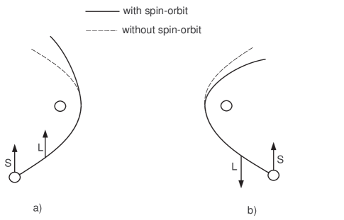
Figure 3: Scattering of a particle with spin $S$ on a spinless target. The collision defines the angular momentum $L$. In a) $S$ and $L$ parallel, reducing the attractive nuclear force. In b) $S$ and $L$ are antiparallel, increasing the attractive nuclear force. Without the spin-orbit term trajectories a) and b) would be indistinguishable.

2.3 Polarization Formalism

Every deuteron has spin. Furthermore, this spin must be aligned in one of three ways with respect to a quantization axes. The spin can be aligned parallel ($m_{I}=1$), anti-parallel ($m_{I}=-1$), or perpendicular ($m_{I}=0$) to this quantization axis.

The polarization formalism given below is based on articles by Ohlsen [8, 9] and describes the relation between all quantities involved in this project. It describes how quantum mechanics, experimental and theoretical nuclear physics meet. This formalism allows one to derive few simple equations (Eq. (11) & Eq. (2.3.3)) that are used to determine beam polarization in terms of known analyzing powers and measured experimental asymmetries.

Although deuterons are spin-1 particles, I will start the polarization formalism for spin-$\frac{1}{2}$ particles then extend it to spin-1 particles. The reason is that, the polarization formalism for spin-$\frac{1}{2}$ particles contains all the essential features of the formalism with much less mathematics. Therefore it is a good starting point to visualize.

2.3.1 Coordinate System

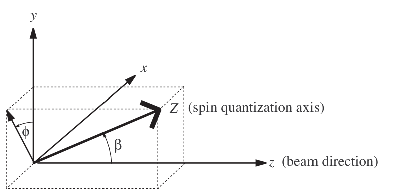
Figure 4: Coordinate system used to describe scattering with a polarized beam.

The coordinate system most often used to describe polarization experiments is called the ‘Madison Convention’ [10] and is shown in Fig. 4. This coordinate system incorporates both beam and scattering parameters into one coordinate system. The direction of the $z$-axis is parallel to the momentum of the incoming beam, k_in. The $y$-axis is along k${}_{in}\times$ k_out, where k_out is the direction of the outgoing ejectile. The $y$-axis, therefore, is perpendicular to the scattering plane. The $x$-axis is left to form a right-handed system with the $y$ and $z$ axes. The angle between $z$ and $Z$ is given by $\beta$. The angle $\phi$ is between $y$ and the projection of $Z$ onto the $x$-$y$ plane. Scattering to the the left, right, up and down with respect to the quantization axis correspond to $\phi=$ 0, 180, 270 and 90^∘ respectively.

Note that $z$ (lower-case) is the beam direction, while $Z$ (upper-case) is the quantization axis direction. One must distinguish between $p_{z}$ and $P_{Z}$. The former is the component of polarization along the the beam direction, while the latter is the degree of polarization along the quantization axis, the quantity of interest in this experiment.

2.3.2 Spin-$\frac{1}{2}$ Particles

A spin-$\frac{1}{2}$ particle can be represented by a Pauli spinor,

$$\chi=\left(\begin{array}[]{c}a_{1}\\ a_{2}\\ \end{array}\right)=a_{1}\left(\begin{array}[]{c}1\\ 0\\ \end{array}\right)+a_{2}\left(\begin{array}[]{c}0\\ 1\\ \end{array}\right),$$ (2)

where $a_{1}$ is the probability amplitude of finding the particle in the state $\left(\begin{array}[]{c}1\\ 0\\ \end{array}\right)$ called spin-up, and $a_{2}$ is the probability amplitude of finding the particle in the spin-down state $\left(\begin{array}[]{c}0\\ 1\\ \end{array}\right)$.

The spin state of an ensemble of $N$ such particles can be represented by a set of Pauli spinors,

$$\chi^{(n)}=\left(\begin{array}[]{c}a_{1}^{(n)}\\ a_{2}^{(n)}\\ \end{array}\right)\qquad n=1,\ldots,N\,,$$

where $n$ runs through all particles.

If the order of spins in an ensemble is not important, but only the average spin, then a beam can be described by a density matrix,

$$\rho=\left(\begin{array}[]{cc}\sum_{n=1}^{N}|a_{1}^{(n)}|^{2}&\sum_{n=1}^{N}a_{1}^{(n)}\,a_{2}^{(n)*}\\ \sum_{n=1}^{N}a_{2}^{(n)}\,a_{1}^{(n)*}&\sum_{n=1}^{N}|a_{2}^{(n)}|^{2}\\ \end{array}\right).$$ (3)

A density matrix fully characterizes the polarization (magnitude and direction) of particle beams.

Here are some relations,

$$p_{x} = Tr(\rho\,\sigma_{x})=\frac{1}{N}\sum_{n=1}^{N}2\,Re(a_{1}^{(n)}\,a_{2}^{(n)*}),$$

$$p_{y} = Tr(\rho\,\sigma_{y})=\frac{1}{N}\sum_{n=1}^{N}2\,Im(a_{1}^{(n)}\,a_{2}^{(n)*}),$$ (4)

$$p_{z} = Tr(\rho\,\sigma_{x})=\frac{1}{N}\sum_{n=1}^{N}(|a_{1}^{(n)}|^{2}-|a_{2}^{(n)}|^{2}).$$

One can show [8] that the density matrix can be written as a linear combination of Pauli spin operators,

$$\rho=\frac{1}{2}\,(I+\sum_{j=1}^{3}p_{j}\,\sigma_{j}),$$ (5)

where:

• $p_{j}$ ’s are the components of polarization in the $x$, $y$, and $z$ directions;

• $I$ is the unit matrix $\left(\begin{array}[]{cc}1&0\\ 0&1\\ \end{array}\right);$

• $\sigma_{j}$ ’s are the Pauli spin operators;
  
  $\sigma_{x}=\left(\begin{array}[]{cc}0&1\\ 1&0\\ \end{array}\right);$ $\sigma_{y}=\left(\begin{array}[]{cc}0&-i\\ i&0\\ \end{array}\right);$ $\sigma_{z}=\left(\begin{array}[]{cc}1&0\\ 0&-1\\ \end{array}\right).$
  

A nuclear reaction can transform the spin state of particles. Therefore, the spinor of an outgoing particle $\chi_{f}$ is related to the spinor of an incoming particle $\chi_{i}$ by a transformation, $M$,

$$\chi_{f}=M\,\chi_{i}\,.$$

$M$ is a $2\times 2$ matrix whose elements are functions of energy and angle.

The density matrix describing the incoming beam $\rho_{i}$ can be written in terms of spinors as

$$\rho_{i}=\sum_{n=1}^{N}\chi_{i}^{(n)}[\chi_{i}^{(n)}]^{\dagger},$$

and for the outgoing beam,

$$\rho_{f}=\sum_{n=1}^{N}\chi_{f}^{(n)}[\chi_{f}^{(n)}]^{\dagger}.$$

The density matrix is transformed by a reaction as

$$\rho_{f}=M\,\rho_{i}\,M^{\dagger}.$$ (6)

The cross section of the reaction can be given by,

$$\sigma(\theta,\phi)=\frac{Tr(\rho_{f})}{Tr(\rho_{i})}=\frac{Tr(M\,\rho_{i}\,M^{\dagger})}{Tr(\rho_{i})}\,.$$ (7)

If the beam is unpolarized

$$\rho_{i}\propto\left(\begin{array}[]{cc}1&0\\ 0&1\\ \end{array}\right),$$

and if the density matrix is normalized to unity

$$\rho_{i}=\frac{1}{2}\left(\begin{array}[]{cc}1&0\\ 0&1\\ \end{array}\right),$$

then Eq. (7) reduces to

$$\sigma_{0}=\frac{1}{2}Tr(M\,M^{\dagger})\qquad\textrm{(unpolarized beam)}.$$

Applying Eq. (6) to Eq. (5) one gets,

$$\rho_{f}=\frac{1}{2}M\,M^{\dagger}+\frac{1}{2}\sum_{j=1}^{3}p_{j}\,M\sigma_{j}M^{\dagger}.$$

Taking the trace yields

$$\sigma(\theta,\phi)=Tr(\rho_{f})=\sigma_{0}\big{(}1+\sum_{j=1}^{3}p_{j}\,A_{j}(\theta)\big{)},$$ (8)

where

$$A_{j}=\frac{Tr(M\sigma_{j}M^{\dagger})}{Tr(MM^{\dagger})}\qquad j=x,y,z.$$

$M$ is the same $2\times 2$ matrix that was used to transform the spin state in Eq. (2) and density matrix in Eq. (6). $A_{j}$’s are the analyzing powers of the reaction. The analyzing powers, like cross section, are a property of nuclear reactions. They can be calculated from theory or measured experimentally.

Parity and time reversal arguments [8] reduce Eq. (8) for two-body reactions to

$$\sigma(\theta,\phi)=\sigma_{0}(1+p_{y}\,A_{y}(\theta)).$$ (9)

This implies that reactions are only sensitive to polarization along the $y$-axis. Polarization along the $x$, or $z$ direction do not affect the cross section.

Since $p_{y}=\vec{P_{Z}}\cdot\vec{y}=P_{Z}\cos\phi$,   Eq. (9) can be written as

$$\sigma(\theta,\phi)=\sigma_{0}\big{(}1+P_{Z}\cos\phi\,A_{y}(\theta)\big{)},$$ (10)

which is plotted in Fig. 5 .

Figure 5: Azimuthal angle dependence of the cross section for $P_{Z}=1$ and $A_{y}=0.5$ . In this example there are more particles going to the left direction than to the right direction. Detectors placed in these directions measure an asymmetry.

Scattering to the left of the quantization axis ($\phi=0$) has a cross section

$$\sigma_{L}=\sigma_{0}(1+P_{Z}\,A_{y}).$$

A detector placed in this direction will measure a count proportional to this cross section

$$L\propto\sigma_{L}.$$

Scattering to the right of the quantization axis ($\phi=180$) would have a cross section of,

$$\sigma_{R}=\sigma_{0}(1-P_{Z}\,A_{y}).$$

A detector placed in this direction will measure a count proportional to

$$R\propto\sigma_{R}.$$

Define the asymmetry, $\epsilon_{1}$, of the reaction as,

$$\epsilon_{1}\equiv\frac{L-R}{L+R}.$$

The asymmetry is, therefore, the difference over the sum of the number of particles detected in the left and right detectors.

Scattering in a direction parallel to the quantization axis has the same cross section as scattering in an anti-parallel direction. Therefore two detectors placed above and below the scattering will measure the same number of ejectiles, resulting in no asymmetry.

It can be seen that

$$P_{Z}\,Ay=\epsilon_{1}.$$ (11)

This equation relates the polarization, analyzing power, and asymmetry for a spin-$\frac{1}{2}$ beam. We introduced this equation in Sec. 1.4, and now present it with subscripts reflecting some of the geometry behind the scattering.

2.3.3 Spin-1 Particles

The cross section of a reaction using a spin-1 polarized beam is

$$\sigma(\theta,\phi)=\sigma_{0}\Big{(}1+\frac{2}{3}p_{y}A_{y}(\theta)+\frac{3}{2}p_{xz}A_{xz}(\theta)\\ +\frac{1}{3}p_{xx}A_{xx}(\theta)-\frac{1}{3}p_{yy}A_{yy}(\theta)+\frac{1}{3}p_{zz}A_{zz}(\theta)\Big{)}.$$

This equation is the spin-1 analogy of Eq. (9). Yet it contains noticeably more terms!

By expressing the polarization in terms of the coordinates ($P_{Z},P_{ZZ},\beta,\phi$) instead of ($p_{y},p_{xz},p_{xx},p_{yy},p_{zz}$) we get,

$$\sigma(\theta,\phi)=\sigma_{0}\Big{(}1+\frac{3}{2}P_{Z}A_{y}(\theta)\cos\phi\sin\beta-P_{ZZ}A_{xz}(\theta)\sin\beta\cos\beta\sin\phi\\ -\frac{1}{4}P_{ZZ}\big{(}A_{xx}(\theta)-A_{yy}(\theta)\big{)}\sin^{2}\beta\cos 2\phi+\frac{1}{4}P_{ZZ}A_{zz}(\theta)\big{(}3\cos^{2}\beta-1\big{)}\Big{)}.$$

In the spin-$\frac{1}{2}$ case, only one polarization ($P_{Z}$) and one analyzing power ($A_{y}$) enter the equations, while for spin-1 beams, two polarizations ($P_{Z}$, $P_{ZZ}$) and four analyzing powers ($A_{y}$, $A_{xz}$, $A_{xx}-A_{yy}$, $A_{zz}$) enter the equations. This complexity arises because a spin-1 beam has three spin substates, while a spin-$\frac{1}{2}$ beam only two (spin up and spin down).

It is worth mentioning that quantities with one index are called vectors, while quantities with two indices are called tensors. For example, $P_{Z}$ is called ‘vector polarization’, and $A_{zz}$ is one of the three ‘tensor analyzing powers’.

Scattering to the left, right, up, and down ($\phi=$ 0^∘, 180^∘, 270^∘, 90^∘) directions with respect to the quantization axis have cross sections,

$$\sigma_{L} = \sigma_{0}(1+\frac{3}{2}P_{Z}A_{y}(\theta)\sin\beta+\frac{1}{2}P_{ZZ}(A_{yy}(\theta)\,\sin^{2}\beta+A_{zz}\,\cos^{2}\beta)),$$

$$\sigma_{R} = \sigma_{0}(1-\frac{3}{2}P_{Z}A_{y}(\theta)\sin\beta+\frac{1}{2}P_{ZZ}(A_{yy}(\theta)\,\sin^{2}\beta+A_{zz}\,\cos^{2}\beta)),$$

$$\sigma_{U} = \sigma_{0}(1+P_{ZZ}A_{xz}(\theta)\sin\beta\cos\beta+\frac{1}{2}P_{ZZ}(A_{xx}(\theta)\,\sin^{2}\beta+A_{zz}\,\cos^{2}\beta)),$$

$$\sigma_{D} = \sigma_{0}(1+P_{ZZ}A_{xz}(\theta)\sin\beta+\frac{1}{2}P_{ZZ}(A_{yy}(\theta)\,\sin^{2}\beta\cos\beta+A_{zz}\,\cos^{2}\beta)).$$

Detectors placed in these scattering directions will measure a count ($L$, $R$, $U$, $D$) proportional to the cross sections,

$$L \propto \sigma_{L}$$

$$R \propto \sigma_{R}$$

$$U \propto \sigma_{U}$$

$$D \propto \sigma_{D}.$$

One defines the five asymmetries $\epsilon_{1}$, $\epsilon_{2}$, $\epsilon_{3}$, $\epsilon_{4}$, $\epsilon_{5}$, by the following equations

$$\epsilon_{1} \equiv \frac{L-R}{L+R}=\frac{\frac{3}{2}P_{Z}\sin\beta\,A_{y}}{1+\frac{1}{2}P_{ZZ}[\sin^{2}\beta A_{yy}+\cos^{2}\beta A_{zz}]}$$

$$\epsilon_{2} \equiv \frac{U-D}{U+D}=\frac{P_{ZZ}\sin\beta\,\cos\beta\,A_{xz}}{1+\frac{1}{2}P_{ZZ}[\sin^{2}\beta A_{xx}+\cos^{2}\beta A_{zz}]}$$

$$\epsilon_{3} \equiv \frac{2(L-R)}{L+R+U+D}=\frac{\frac{3}{2}P_{Z}\sin\beta\,A_{y}}{1+\frac{1}{4}P_{ZZ}[3(\cos^{2}\beta-1)A_{zz}]}$$ (12)

$$\epsilon_{4} \equiv \frac{2(U-D)}{L+R+U+D}=\frac{P_{ZZ}\sin\beta\,\cos\beta\,A_{xz}}{1+\frac{1}{4}P_{ZZ}[3(\cos^{2}\beta-1)A_{zz}]}$$

$$\epsilon_{5} \equiv \frac{(L+R)-(U+D)}{L+R+U+D}=\frac{-\frac{1}{4}P_{ZZ}\sin^{2}\beta\,\,(A_{xx}-A_{yy})}{1+\frac{1}{4}P_{ZZ}[3(\cos^{2}\beta-1)A_{zz}]},$$

which relate the asymmetries, analyzing powers, and polarizations for spin-1 beams. These are the generalization from spin-$\frac{1}{2}$ (Eq. (11)) to spin-1 particles.

2.4 $d+d$ Reactions

What happens when a deuteron beam strikes a deuteron target? Many things happen, so let’s restrict the question to: What nuclear reactions are possible when a deuteron beam strikes a deuteron target? Table 1 lists all known reactions.

Reaction type	Reaction	Q-value (MeV)
Elastic scattering	D$(d,d)$D	0
One-particle rearrangement	D$(d,n)^{3}$He	3.27
	D$(d,p)^{3}$H	4.03
Radiative capture	D$(d,\gamma)^{4}$He	23.8
Breakup reaction	D$(d,n)p$ D	-2.2

Table 1: $d+d$ nuclear reactions.

A number of reaction listed in Table 1 take place in the center of the sun, and possibly in future fusion reactors. Coincidentally, solar and reactor plasmas are in the same energy range as in this experiment. Yet this setup is used to measure polarization, and not to study solar plasmas.

The cross section of the D$(d,n)^{3}$He reaction highly depends on the incident deuteron energy, as is shown in Fig. 6. A simple quantum mechanical effect can model this dependence satisfactorily, as is explained below.

The potential between two nuclei is attractive at short distances (a few fm) because of the strong force, and repulsive at large distances (greater than a few fm) because of the coulomb force. A deuteron approaching another deuteron sees a potential barrier with a height of about 1 MeV. How can a deuteron with kinetic energy in keV range get through the barrier to fuse with the other deuteron? The answer is quantum mechanical tunnelling! The tunnelling probability, hence the cross section, is proportional to

$$\sigma(E)\propto e^{\frac{-1}{\sqrt{E}}}$$ (13)

This dependence is called the ‘Gamov factor’. Fitting it to published data sets [11] of D$(d,n)^{3}$He cross sections yields an empirical relation,

$$\sigma(E)=a\,e^{\frac{-b}{\sqrt{E}}}$$ (14)

with $a=22\pm 4$  mb and $b=30\pm 2\,\sqrt{\textrm{keV}}$.

Figure 6: Energy dependence of the D$(d,n)^{3}$He cross section. Fit of a Gamov model to data points from various experiments.

2.5 Stopping Power

The basis of any understanding in experimental nuclear and particle physics depends on the understanding of the ‘passage of radiation though matter’. Instances of ‘passage of radiation through matter’ are; an alpha beam impinging on a gold foil (Rutherford’s famous experiment), a neutron depositing energy in a detector (as in this experiment), and ion radiotherapy (where ion beams destroy tumors).

As charged particles pass through matter they lose energy and are deflected. This is not surprising in light of the many imaginable ways in which particle and matter can interact. The most important phenomena that contribute to the net process are

1. Inelastic collisions with atomic electrons

2. Elastic scattering from nuclei

3. Inelastic nuclear reactions

4. Cherenkov radiation

5. Bremsstrahlung

6. etc …

A formula which models these phenomena is the well-known Bethe-Bloch formula [12]. This semi-empirical formula gives the energy loss ($\frac{dE}{dx}$) of various charged particles though various materials. With the energy loss—also called stopping power—one can calculate the range of particles and total energy deposited in matter. These quantities are vital for detector and safety consideration, since you want to know where your particles are going and with how much energy! Although the Bethe-Bloch formula for stopping power is extensively used in nuclear physics, it is only valid for particles with energies greater than 1 MeV/nucleon. At the low energies of this experiment another model and formula for stopping power is given by Lindhard [13], which states that the stopping power is proportional to the beam velocity

$$\frac{dE}{dx}\propto v\propto\sqrt{E}.$$ (15)

Anderson [14] has compiled empirical formulas for stopping powers of various beam and target combinations, by fitting data with the Bethe-Bloch and Lindhard formulas. The stopping power of a deuteron beam on a C₂D₄ target is given by

$$\frac{dE}{dx}=14.48\,E^{0.45}\qquad\textrm{($[E]=$ keV and $[x]=\mu$m).}$$ (16)

Calculation of the mean penetration depth of the beam into the target yields 0.4 to 0.7 $\mu$m for $E_{d}=$ 25 to 80 keV. This is the distance within which the mean beam energy decreases to zero. Since many relevant parameters—such as cross section and analyzing power—are energy dependent, their average value has to be calculated. The cross section is energy dependent, and since there is an energy loss of the beam through the target, therefore the average cross section must be calculated.

The Bethe-Bloch Formula does not apply to neutral particles such as photons and neutrons. Neutral particles have a larger range through matter than charged particles. Particles created from a $d+d$ reaction, at these energies, include neutrons ($n$), protons ($p$), tritons (³H), helium-3 (³He), helium (⁴He), and $\gamma$-rays. $\gamma$-rays are also observed from the de-excitation of nuclei after having absorbed neutrons. Therefore, wherever one observes neutrons, one is likely to observe $\gamma$-rays as well. The charged particles ($p$, ³H, ³He, and ⁴He) do not make it out of the vacuum chamber. They are stopped in the glass beam tube, metal target holder, or the target itself due to their small range of order order $\mu$m to mm. This tiny range is due to the high energy loss of low energy charged particles passing through matter. Neutral particles, on the other hand, such as neutrons and $\gamma$-rays, do not interact as much with material and are able to exit the beam tube and reach the detectors or go beyond them. This is why the D($d,n$)³He reaction was chosen, because it could be isolated from other reactions also occurring.

3 Experimental Set-Up

The different devices of our experiment are sketched in Fig. 7.

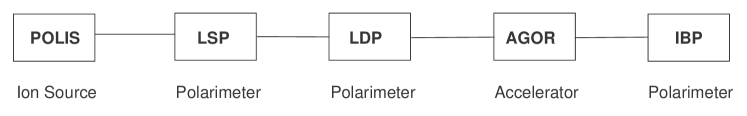
Figure 7: Schematics of the beam line we used. Polarized beams are created by POLIS, the beam polarization is measured with the LSP and the LDP, the beam is accelerated, and finaly the beam polarization is measured with the IBP.

We briefly describe POLIS. We describe at length the components of the LDP. The LSP [15, 16], AGOR [17], and the IBP[18] are described elsewhere.

3.1 Polarized Ion Source

Our Polarized Ion Source [19] (POLIS) provides beams of polarized protons or deuterons. Proton beams can be vector polarized, while deuteron beams can be vector and/or tensor polarized.

Before the invention of polarized ion sources, such as POLIS, polarized beams were produced by using the scattered ejectiles of a reaction. These ejectiles were partly polarized, and were used themselves as a beam for another experiment. These ‘double scattering’ experiments were plagued by low polarization and intensity.

The production of a polarized deuteron beam from POLIS is outlined as follows,

$\rm{D}_{2}\xrightarrow{dissociation}D\xrightarrow{transitions}D^{*}\xrightarrow{ionization}$ $\overrightarrow{d}$

First, deuterium molecules from a gas cylinder are dissociated into deuterium atoms and collimated into a beam. Then, electromagnetic transitions polarize the atom by populating some of its hyperfine states. The polarized atoms are ionized leaving only a beam of polarized deuteron nuclei. This beam is then accelerated to desired energies, and steered to a particular experiment.

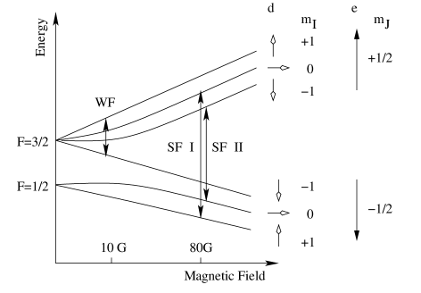
Figure 8: Breit-Rabi diagram of a deuterium atom in the ground state. The spin substate of the nucleus (d) and its electron (e) are listed on the right of the figure.

Each hyperfine state of an atom represents a particular alignment of the spin of the nucleus and electrons. The electromagnetic transitions between hyperfine states are produced by applying RF fields to atoms present in a magnetic field, as depicted in Fig. 8. POLIS has four transitions units called Weak Field, Medium Field, Strong Field I, and Strong Field II. Different combination of these transition units populates different hyperfine states. Populating a particular hyperfine states is selecting a spin substate of the nucleus and electrons. The spin substate of electrons is irrelevant since electrons are stripped from the atom. The spin substate of the nuclei constitute the beam polarization.

POLIS	Max. Theoretical		Beam
Transition	Polarization		Polarization
Units	$P_{Z}$	$P_{ZZ}$
WF	$-2/3\quad$	0	Positive Vector
SF. I + SF. II	$2/3$	0	Negative Vector
MF + sextupole + SF. I	0	1	Positive Tensor
MF + sextupole + SF. II	0	-2	Negative Tensor

Table 2: POLIS transition units with the beam polarization they generate. Other combination of transition units are possible yielding beams with both non-zero $P_{Z}$ and $P_{ZZ}$.

3.2 Low Energy Deuteron Polarimeter

The LDP consists of a target and four detectors as shown in Fig. 9. A polarized deuteron beam from POLIS impinges on a target containing deuteron in the form of C₂D₄ to reacts as D($\vec{d},n$)³He sending neutrons in space.

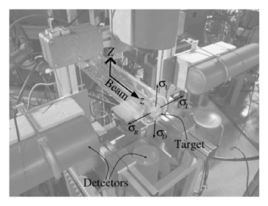
Figure 9: Photograph of the LDP showing beam tube, target holder and four neutron detectors. Also shown are the directions of the beam, the quantization axis, and left, right, up, and down scattering.

3.2.1 Target

A deuterated-polyethylene (C₂D₄) film was used as a deuterium target. It has the same chemical properties as polyethylene (i.e. the hydrocarbon C₂H₄), except that it contains deuterium nuclei (deuterons) instead of hydrogen nuclei (protons). Although carbon is present in the target material, it does not produce neutrons in a nuclear reaction because the Q-value of the ¹²C($d,n$)¹³N reaction ($Q=-281$ keV) is higher than our beam energy. Therefore neutrons detected originate exclusively from the D($d,n$)³He reaction. Alternative targets to C₂D₄ exist, such as, deuterated-titanium, or deuterium gas targets. These were not used because C₂D₄ targets were readily available at the KVI and are more convenient to produce. Target thickness was in the order of a few hundred $\mu$g/cm², which corresponds to a target depth of a few $\mu$m.

At early stages of the experiment, targets consisted of a C₂D₄ thin film held by a rectangular frame. Eventually targets evolved into a C₂D₄ thin film on a round metal backing. There were two problems with the initial target design. First, the target would melt under beam heating. The reason was that Polyethylene, being a plastic, conducts poorly the energy deposited by the beam. The solution was to couple the thin-film to a metallic backing acting as a heat sink. Secondly, the sharp edges of the rectangular frame help produce unwanted electrical discharge when the target was at High Voltage. A round metal holder increased the breakdown voltage. The breakdown voltage was found to be proportional to the pressure in the evacuated beam line, the deuteron beam current, and surface conditions on the target.

3.2.2 Detectors

The detectors we used were ‘liquid organic scintillators’ of type NE213. These detectors are frequently used for the detection of neutrons. The signal produced by these detectors depends on the type of particle entering them.

3.2.3 Pulse Shape Discrimination

As determined earlier (Sec. 2.5 and 2.4), only neutrons and $\gamma$-rays will reach the detectors. One wants to distinguish between detected neutrons and $\gamma$-rays because one needs to measure the asymmetry originating from a single reaction, and not two reactions. In our case neutrons should be counted, while $\gamma$-rays should be rejected. A method called Pulse Shape Discrimination [12, 20] allows different particles to be distinguished based on the signal they produce in detectors. Different particles have different energy loss mechanisms inside matter, and so produce sightly different signal shapes. Neutrons will deposit their energy more slowly than gamma-rays, therefore the signal they create decays more slowly. The signals are illustrated in Fig. 10.

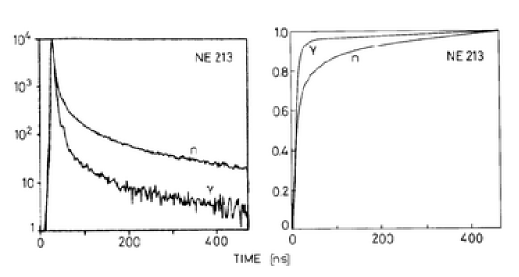
Figure 10: Pulse shape differences for neutron and $\gamma$-rays. Detector signals are shown on the right panel and the integral of the signals on the left panel.

By monitoring the signal shape which the detected particles produce, one can identify particles. We monitored the signal shape by integrating two copies of the signal with two different time intervals, and taking their ratio. The signal and time intervals are illustrated in Fig. 11.

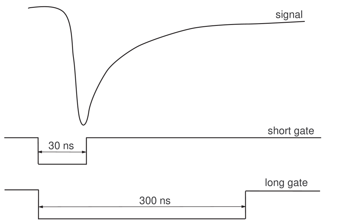
Figure 11: Detector signal and integration gates as used in our experiment.

The ratio of these two integrated quantities is proportional to the decay time of the signal, and is the basis for particle identification. By plotting the occurrence of signals as a function of this ratio we get a pulse shape spectrum as shown in Fig. 12.

Figure 12: Pulse shape spectrum for one detector. Neutrons are well separated from a large background of $\gamma$-rays. The number of neutrons detected is the number of events under the neutron peak.

We can also plot the integral of the signal with the long gate versus that with the short gate to get a 2-D scatter plot of pulse shapes, as shown in Fig. 13.

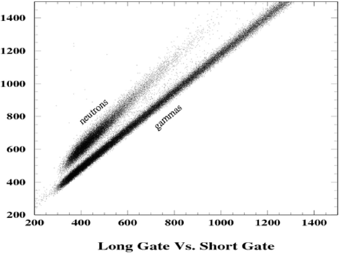
Figure 13: 2-D pulse shape spectrum. Detected neutrons can clearly be separated from detected $\gamma$-rays.

3.2.4 Post Acceleration

Placing the target at a potential is an experimental trick to reduce the measuring time of our experiment. The cross section of the D$(d,n)^{3}$He reaction was found to depend on the reaction energy (Fig. 6). By increasing the energy of the beam, the cross section, therefore reaction rate, increases. High counting rates have the obvious advantage of lower statistical uncertainty for a given measuring time. The maximum beam energy that POLIS can produce is 30 keV. Placing the target at negative potentials will accelerate the positively charged deuteron beam. If the beam is initially at 30 keV and the target at $-50$ kV, then the beam energy as it reaches the target is 80 keV. The reaction rate at 80 keV is about an order of magnitude higher than at 30 keV!

Post acceleration equipment is not shown in the photograph of the LDP (Fig. 9). It consists of nothing more than a high voltage cable connecting the target to a high voltage power supply surrounded by safety features (insulation and grounding).

3.2.5 Data Acquisition

Data acquisition consists of electronic modules, a CAMAC crate, and a PC. Electronic modules can manipulate and perform basic operations on electronic signals. The detector signal was first split into multiple copies by a ‘fan-in/fan-out’ unit. Two copies of the signal were each put into a ‘constant fraction discriminator’ (CFD) unit to generate logical gates. One long and one short gate acts as integration windows for the detector signal as shown in Fig. 11. Another copy of the signal was cable delayed before being put to a ‘charge to digital converter’ (QDC) units along with the short and long gate. The QDC integrates the voltage of a signal and converts it to into a binary string which can be read by a PC. The program DAX, based on the CERN Program Library package [21], was used to write raw data into event files (*.ntuple). PAW [22] was used to perform a simple analysis of the data such as plotting and counting.

4 Data Analysis

4.1 Low-Energy Deuteron Polarimeter

4.1.1 Analyzing Powers

Analyzing powers are a manifestation of the dependence of the reaction cross section on spin. The analyzing powers relevant to this experiment are almost entirely available in the literature. Becker [23] has measured all analyzing powers ($A_{y}$, $A_{xz}$, $A_{zz}$, $A_{xx}-A_{yy}$) for the D$(d,n)^{3}$He and D$(d,p)^{3}$H reactions at the reaction energy of $E=28$ keV. Fletcher [24, 25] has measured two tensor analyzing powers ($A_{zz}$, $A_{xx}-A_{yy}$) of both reactions at the beam energies of $E_{d}=$ 25, 40, 60, and 80 keV. Tagashi [26] has measured all analyzing powers of the D$(d,p)^{3}$H reaction at $E_{d}=$ 30, 50, 70, and 90 keV. Our polarimeter is limited to the energy range of $E_{d}=$ 25 to 80 keV, because that is the energy range at which analyzing powers are presently known, also because those are the beam energies available to us.

$A_{xz}$ and the energy dependence of $A_{y}$ are not published. $A_{y}$ is claimed [23] to be energy independent in our energy range. Furthermore, $A_{y}$, for the D$(d,p)^{3}$H reaction, has negligible energy variation as can be seen from [26]. An unknown $A_{xz}$ is not a problem for us since we do not use it in our analysis. When $\beta=90^{\circ}$ (as in our setting of the beam) only $\epsilon_{1}$, $\epsilon_{3}$, and $\epsilon_{5}$ enter the analysis (Eq. 2.3.3).

Analyzing powers are usually reported in the literature as data points with fitted curve (Fig. 14) as in [23, 25], or just fitted curves (Fig. 15) as in [24, 26]. The fitting functions are Legendre polynomials.

Figure 14: Data and fit of $A_{y}$ at 28 keV from Becker [23].

Figure 15: Fit of $A_{zz}$ at various beam energies from Fletcher [25].

4.1.2 Effective Analyzing Powers

In our analysis one cannot directly use the analyzing powers as found in the literature. The asymmetries measured by the detectors are the convolution of both non-zero analyzing powers and experimental effects, such as:

1. Finite acceptance of the detectors. Detectors cover a non-zero solid angle. Therefore, the analyzing power must be averaged over this solid angle. We chose to average $A(\theta)$ over $\Delta\theta$, and disregard $\Delta\phi$ effects because they are small at $\theta_{lab}=90^{\circ}$.

2. Change in analyzing power due to the energy loss of the beam through the target, $A(E)$. Fig. 15 shows that $A_{zz}$ is energy dependent.

3. Change in cross section due to energy loss of the beam though the target, $\sigma(E)$.

4. Energy profile of the beam through the target; $E(x)$.

These experimental effects give rise to an effective analyzing power given by

$$A^{eff}=\frac{\int_{\Delta\theta}\int_{\Delta x}A\big{(}E(x),\theta\big{)}\,\,\sigma\big{(}E(x)\big{)}\,d\theta\,dx}{\Delta\theta\ \int_{\Delta x}\sigma\big{(}E(x)\big{)}\,dx}.$$ (17)

The opening angle of each of our detectors is $\Delta\theta=26^{\circ}$. $\Delta x$ is the range of the beam. $E(x)$ and $\Delta x$ can be calculated from the stopping power of a deuteron beam on a C₂D₄ target (Eq. (16), $E(0)=E_{d}$ and $E(range)=0$). $A(E,\theta)$ represents the energy and polar angle dependence of any of the four analyzing powers ($A_{y}$, $A_{xz}$, $A_{zz}$, $A_{xx}-A_{yy}$). $A(\theta$) is given in the literature. $A(E)$ was estimated by fitting a quadratic polynomial through the four energies at which analyzing powers are known.

The effective analyzing powers at two different beam energies are given in Table 3.

	$E_{d}=$ 50 keV	$E_{d}=$ 80 keV
$A_{y}^{eff}$	$0.186\pm 0.01$	$0.186\pm 0.01$
$A_{zz}^{eff}$	$0.31\pm 0.03$	$0.25\pm 0.03$
$(A_{xx}-A_{yy})^{eff}$	$-0.98\pm 0.1$	$-0.83\pm 0.1$

Table 3: Effective analyzing power of the LDP for 50 and 80 keV beams.

4.1.3 Instrumental Asymmetries

Fig. 16 shows the neutron peaks in each detector coming from the reaction with a polarized and unpolarized beam.

Figure 16: Neutron peak in each of the LDP’s detectors. The dashed line stems from an unpolarized beam, whereas the solid line stems from a positive vector polarized beam.

One can observe that the neutron peaks with an unpolarized beam are not of the same height, indicating asymmetries! For example, the peak of the Right and Up detector approach 2000 neutrons per bin, while the Left and Down peaks approach 1000 neutrons. This is due to instrumental asymmetries. One should distinguish between reaction asymmetries and instrumental asymmetries. Reaction asymmetries are fundamental and due to a non-zero analyzing power of the nuclear reaction. Instrumental asymmetries are due to mismatches in detector response, such as differences between detectors in, gain, solid angle, detection efficiency, discriminator threshold level, or signal shape. The fact that instrumental asymmetries are equal to a factor of 2 here, indicates that the detector responses were not matched properly. This is not a problem because one uses unpolarized beams to quantify instrumental asymmetries. Unpolarized beams theoretically do not create reaction asymmetries. Therefore, any asymmetry measured with unpolarized beams is taken to be instrumental asymmetries. Normalizing the detector counts obtained with polarized beams, by counts obtained from unpolarized beams, leaves only the reaction asymmetries needed to determine beam polarization. Therefore, for the right detector, the number of neutrons creating reaction asymmetries is,

$$R=\frac{R_{polarized}}{R_{unpolarized}}.$$

And similarly for the other three detectors $L$, $U$, and $D$.

Until this point, we have covered the effective analyzing powers and the normalized asymmetries. Using Eq. (2.3.3), one solves a system of equations to get the unknowns ($P_{Z}$, $P_{ZZ}$).

4.1.4 Sample Calculation

As an example of the procedure to calculate the polarization from neutron counts, we analyze the data presented in Fig. 16.

$$R = {62566}/{51124}=1.22380,$$

$$L = {25815}/{26985}=0.95664,$$

$$U = {56244}/{51337}=1.0955,$$

$$D = {26600}/{23455}=1.1340.$$

With the asymmetries,

$$\epsilon_{1} = \frac{L-R}{L+R}=0.1225=\frac{0.279\,P_{Z}\sin\beta}{1+\frac{1}{2}P_{ZZ}[-\sin^{2}\beta\,0.647+\cos^{2}\beta\,0.312]}$$

$$\epsilon_{2} = \frac{U-D}{U+D}=-0.0172=\frac{0.0109\,P_{ZZ}\sin\beta\,\cos\beta}{1+\frac{1}{2}P_{ZZ}[\sin^{2}\beta\,0.958+\cos^{2}\beta\,0.312]}$$

$$\epsilon_{3} = \frac{2(L-R)}{L+R+U+D}=0.1211=\frac{0.279\,P_{Z}\sin\beta}{1+0.078\,P_{ZZ}[3(\cos^{2}\beta-1)\,0.312]}$$

$$\epsilon_{4} = \frac{2(U-D)}{L+R+U+D}=-0.0174=\frac{0.0109\,P_{ZZ}\sin\beta\,\cos\beta}{1+0.078\,P_{ZZ}[3(\cos^{2}\beta-1)\,0.312]}$$

$$\epsilon_{5} = \frac{(L+R)-(U+D)}{L+R+U+D}=-0.0111=\frac{0.245\,P_{ZZ}\sin^{2}\beta\,\,}{1+0.078\,P_{ZZ}[3(\cos^{2}\beta-1)\,0.312]}$$

Fixing $\beta=90^{\circ}$ and solving for $P_{ZZ}$ in $\epsilon_{5}$ yields $P_{ZZ}=-0.05$. Solving for $P_{Z}$ in $\epsilon_{3}$ or $\epsilon_{1}$ using $P_{ZZ}$ yields $P_{Z}=0.4$. Applying propagation of errors to these equations with the statistical uncertainty originating from counting uncertainty ($\Delta N=\sqrt{N})$, and the systematic uncertainty originating from the uncertainty in analyzing powers given in Table 3, yields, $\Delta P_{ZZ}^{stat}=0.001$, $\Delta P_{Z}^{stat}=0.003$, $\Delta P_{ZZ}^{sys}=0.005$, and $\Delta P_{Z}^{sys}=0.02$. This measurement of polarization is plotted in Fig. 17.

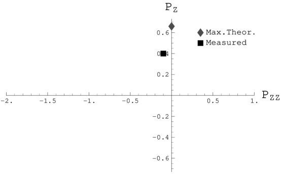
Figure 17: Measured polarization and maximum theoretical polarization for a positive vector polarized beam. The vertical axis is the vector component of polarization, while the horizontal axis is the tensor component. In this plot vector polarized beams lie on, or close to, the vertical axis, while tensor polarized beams lie on, or close to, the horizontal axis.

4.1.5 Low Energy Deuteron Polarimeter

The Low Energy Deuteron Polarimeter (LDP) data are tabulated in Table 4 and plotted as squares in Fig. 18.

POLIS	Detector				Measured
State	Count				Polarization
	R	L	U	D	$P_{Z}\stackrel{{\scriptstyle stat}}{{\pm}}\,\stackrel{{\scriptstyle sys}}{{\pm}}$	$P_{ZZ}\stackrel{{\scriptstyle stat}}{{\pm}}\,\stackrel{{\scriptstyle sys}}{{\pm}}$
WF	30703	43889	22943	51843	$0.49\pm 0.0008\pm 0.03$	$-0.095\pm 0.003\pm 0.005$
ST. I + ST. II	25815	62566	26600	56244	$-0.45\pm 0.001\pm 0.03$	$-0.043\pm 0.003\pm 0.0006$
MF + ST. I	29379	53164	20200	41951	$-0.030\pm 0.001\pm 0.005$	$0.414\pm 0.003\pm 0.05$
MF + ST. II	18011	33064	24853	54641	$-0.008\pm 0.0009\pm 0.002$	$-1.1\pm 0.004\pm 0.1$
Unpolarized	54312	100427	444617	101696	0	0

Table 4: LDP counts and polarizations.

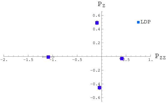
Figure 18: LDP measurements of polarization of four polarized beams. Systematic error bars are just visible, while statistical error bars are smaller than the symbol size.

4.2 In-Beam Polarimeter

The In-Beam Polarimeter (IBP) measures similarly to the LDP. Namely, by measuring asymmetries and exploiting known analyzing powers. The reaction used to measure asymmetries was H($d,d$)p at $E_{d}=$ 80 MeV. The analyzing powers for this reaction, at this energy, are not reported in the literature, so we used calculated [27] analyzing powers shown in Table  5. The uncertainties in analyzing power ($\approx 3\%$) were taken as the variation in analyzing power between various potentials.

The IBP data are tabulated in Table 6 and plotted as stars in Fig. 19.

	$E_{d}=$ 80 MeV
	$\theta_{cm}=100^{\circ}$
$A_{y}$	$-0.291\pm 0.005$
$A_{zz}$	$-0.74\pm 0.02$
$A_{xx}-A_{yy}$	$-0.107\pm 0.003$

Table 5: IBP analyzing powers.

POLIS	Detector				Measured
State	Count				Polarization
	R	L	U	D	$P_{Z}\stackrel{{\scriptstyle stat}}{{\pm}}\,\stackrel{{\scriptstyle sys}}{{\pm}}$	$P_{ZZ}\stackrel{{\scriptstyle stat}}{{\pm}}\,\stackrel{{\scriptstyle sys}}{{\pm}}$
WF	29589	17220	25004	24368	$0.478\pm 0.0008\pm 0.01$	$-0.443\pm 0.006\pm 0.001$
ST. I + ST. II	13180	20140	18465	18085	$-0.643\pm 0.001\pm 0.008$	$-0.112\pm 0.005\pm 0.004$
MF + ST. I	19407	17626	18181	17932	$-0.131\pm 0.001\pm 0.003$	$0.478\pm 0.007\pm 0.004$
MF + ST. II	10834	10257	13681	13391	$-0.112\pm 0.001\pm 0.002$	$-1.44\pm 0.009\pm 0.01$
Unpolarized	71690	73594	75327	75093	0	0

Table 6: IBP counts and polarizations.

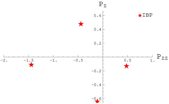
Figure 19: IBP measurement of polarization of four polarized beams. Error bars are not visible.

4.3 Lamb-Shift Polarimeter

The Lamb-Shift Polarimeter (LSP) uses a different technique, than the LDP and IBP, to measure polarization. It measures directly the spin substate distribution of a beam, from which the polarization can easily be obtained.

Figure 20: Spin state distribution of a negative vector polarized beam measured by the LSP.

Let $N_{+}$ be the population of spins in the spin substate $m_{I}=+1$. $N_{0}$ the population of spins in the $m_{I}=0$ state, and $N_{-}$ for $m_{I}=-1$. The polarization in terms of populations is,

$$P_{Z} = \frac{N_{+}-N_{-}}{N_{+}+N_{0}+N_{-}}$$

$$P_{ZZ} = 1-3\frac{N_{0}}{N_{+}+N_{0}+N_{-}}.$$

Populations are calculated by fitting three gaussian peaks and a baseline to the LSP’s spin substate distribution, as is illustrated in Fig. 20. The area under the peaks are equal to the populations $N_{+}$, $N_{0}$, and $N_{-}$. The uncertainty in fitting parameters (obtained from the fitting program) were propagated into uncertainties in polarization. The data shown in Fig. 20 yield $P_{ZZ}=-0.121\pm 0.004$ and $P_{Z}=-0.51\pm 0.01.$ These uncertainties are purely statistical.

The LSP data are tabulated in Table 7 and plotted as triangles in Fig. 21.

POLIS	$P_{Z}$	$P_{ZZ}$
State
WF	$-0.51\pm 0.01$	$-0.121\pm 0.004$
WF	$-0.50\pm 0.01$	$-0.105\pm 0.003$
ST. I + ST. II	$0.52\pm 0.01$	$-0.141\pm 0.005$
ST. I + ST. II	$0.510\pm 0.01$	$-0.144\pm 0.004$
ST. I + ST. II	$0.507\pm 0.003$	$-0.133\pm 0.004$
MF + ST. I	$-0.009\pm 0.009$	$0.68\pm 0.07$
MF + ST. I	$0\pm 0.07$	$0.67\pm 0.07$
MF + ST. II	$0\pm 0.01$	$-1.50\pm 0.05$
MF + ST. II	$0\pm 0.02$	$-1.52\pm 0.05$

Table 7: LSP data, taken within a few minutes of each other.

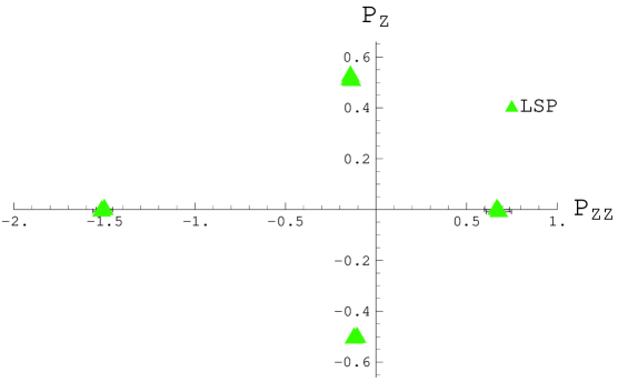
Figure 21: LSP measurement of polarization of four polarized beams.

5 Results

The measurements taken by the three polarimeters in Fig. 18, Fig. 19, and Fig. 21 are superimposed in Fig. 22.

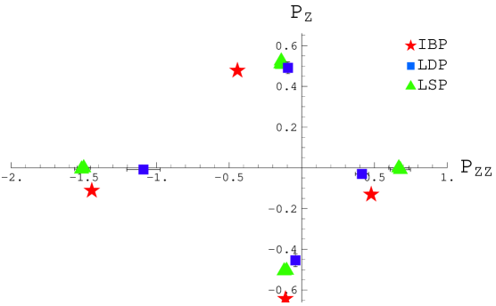
Figure 22: Polarization measurements of all three polarimeters.

These data were collected on the night of 15-16 October 2004. LSP measurements were taken between 10 and 11 pm, IBP measurements were taken between 3 and 5 am, and LDP measurements were taken between 6 and 11 am. The LSP and LDP disagree on the tensor component of polarization, while the LSP and IBP disagree on the vector and tensor components of polarization. It is difficult to draw definitive conclusions from this plot for three reasons:

1. The LDP does not fully agree either with the IBP or LSP, not allowing one to prove whether the polarization changes between LSP and IBP, or if the LSP or IBP have unknown systematic errors.

2. We do not have a big data set with multiple measurements at this moment.

3. We cannot exclude changes in beam polarization while the polarimeters were being switched. Had we monitored the polarization with one polarimeter (LSP) before and after the measurements of other polarimeters, we would know whether the beam polarization was constant over the measurement period.

Repeating the experiment would have been the natural way to proceed, this would have addressed points 2 and 3. Yet because of time and facility constraints, we have to evaluate the present data.

The IBP data are not reliable for two reasons. Firstly, we do not know how successful the theory, which calculates IBP’s analyzing powers, is. Secondly, the asymmetries we measured depended on how we analyzed the data (where we placed cuts). Both of these issues can be addressed with more time. Until then we cannot be confident about the present IBP polarization measurements and uncertainty in polarizations. Therefore we cannot presently answer the question whether there are polarization changes in the accelerator.

One can observe that the polarization measurements of the LSP and LDP agree quite well for the $P_{Z}$ component of polarization but not for $P_{ZZ}$. One can also see that the LDP measures always less $P_{ZZ}$ than the LSP (all LDP points are closer to the vertical axis in Fig. 22).

We can rule out large decreases of $P_{ZZ}$ in time between the LSP and LDP measurements. If the polarization were to change, it must do so in particular ways. If the dissociator of POLIS were to operate anomalously (a decrease in efficiency), then the polarization of both vector and tensor polarized beams would decrease. This is not observed since only the tensor polarized beams have lower polarization. If the medium field transitions units of POLIS (the transition field allowing tensor polarized beams) would operate anomalously, then the polarization would vary diagonally on a $P_{ZZ}$ vs. $P_{Z}$ plot. This is not seen since, $P_{Z}$ of tensor polarized beams is the same for both the LSP and LDP, ruling out variations in the medium field transition unit. We are left with the conclusion that the LDP underestimates the tensor component of beam polarization.

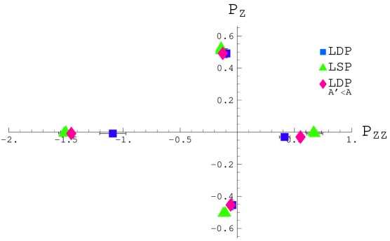
Figure 23: LDP with reduced tensor analyzing powers (diamond symbol) is in better agreement with the LSP.

The agreement between LSP and LDP can be improved if one assumes lower tensor analyzing powers. By reducing the tensor analyzing powers ($A_{xx}-A_{yy}$ and $A_{zz}$) of the LDP by 25%, $P_{ZZ}$ increases as shown in Fig. 23. This suggest that the effective tensor analyzing powers ($(A_{xx}-A_{yy})^{eff}$ and $A_{zz}^{eff}$) we used are wrong. Either because our model (Eq. 17) for effective tensor analyzing power is incomplete, or because the analyzing powers we used in the model were wrong. We used the tensor analyzing powers published by Fletcher [24] for two reasons. Firstly because they were closer to the theoretical value predicted. Secondly because they were published for a number of energies, allowing us to estimate the energy dependence of the analyzing powers, and use beams of any energy between 25 and 80 keV. The tensor analyzing powers published by Becker [23] were not used because they were inconsistent with the theoretical predictions, and also because they were published at a single energy. The difference in tensor analyzing power between these two publications is considerable. For example, at $E_{d}\approx 30$ keV and $\theta_{cm}=90^{\circ}$, Fletcher [24] has $A_{xx}-A_{yy}$ and $A_{zz}$ approximately 35% and 50% greater than Becker [23]. Our effective analyzing powers were derived from Fletcher’s analyzing powers, yet our data would fit better with lower tensor analyzing powers, such as those published by Becker. We could not use Becker’s tensor analyzing powers because our measurements was performed at different energies.

Although $P_{Z}$ depends on the value of $P_{ZZ}$ ($\epsilon_{1}$ in Eq. (2.3.3)), this dependence is very weak. Having the wrong $P_{ZZ}$ changes $P_{Z}$ by a negligible amount.

The vector polarization that the LDP measures is reliable because the vector analyzing power is energy independent, matches the theoretical prediction, and does not depend on our choice of model for effective analyzing powers.

Finally, the LDP measures $P_{Z}$’s of vector polarized beams that are on average 7% lower than the LSP. This relative difference can originate from unknown systematic uncertainties of the LSP or LDP, or because of polarization change in space (between the polarimeters) or in time (between the measurements).

6 Conclusions

We built a Low Energy Deuteron Polarimeter (LDP), based on a reaction that received little attention for polarimetry. We find that the LDP is well suited to measure asymmetries but presently lacks a proper tensor analyzing power calibration.

Data from our polarization cross-check experiment cannot answer whether there are polarization changes during acceleration, because our IBP data are, at this point, preliminary.

The relative difference, of vector polarized beams, between the LSP and LDP was 7% in our experiment.

6.1 Future Improvements

We can point out future improvements to the experiment we performed, and to future versions of the LDP.

6.1.1 Polarimeter Cross-Check Experiment

• The online analysis program of the LSP, although fast, often returns inaccurate polarization and uncertainties in polarization. Offline analysis, which was done here, decreased the uncertainties (sometimes by a factor of 10) and changed the polarization (mostly the tensor component of polarization). The online analysis program could be made more accurate.

• Use all the polarization states that POLIS can provide (13), not just pure vector (2) and tensor beams (2) but mixed vector-tensor beams (9), for additional systematic checks between polarimeters.

• Our conclusions rely to a large extent on the fact that the beam polarization from the source was constant during the experiment. During next experiment the polarization should be monitored with the LSP before and after each run.

6.1.2 LDP

• Find better tensor analyzing powers. Either by improving the model that calculates effective analyzing power, or by using a better data set of published tensor analyzing powers.

• Measure the energy dependence of the vector analyzing power. We expect it to be energy independent, but do not know to what level.

7 Acknowledgement

I would like to thank a number of people. Starting with Johan Messchendorp, my supervisor, who was involved in every aspect of this project. His experience and insight were extremely valuable to me. Nasser Kalantar-Nayestanaki, my professor, for his stimulating and energetic character. Hossein Mardanpour, my colleague, for constantly helping me with computers. Rob Kremers and Hans Beijers for useful discussions. The Few-Body Physics Group for their conviviality. Finally my parents for their support and patience.

References

- [1] N.F. Mott, Proc. R. Soc. London A 124, 425 (1929).
- [2] W. Pauli, Magnetism, Gauthier-Villars, Brussels, 1930, pp. 217-226.
- [3] H. Batelaan, T. Gray, T. J. Schwendiman, Phys. Rev Lett. 79, 4517 (1997).
- [4] W. Glöckle, H. Witała, D. Hüber, H. Kamada, and J. Golak, Physics Reports, 274, 3-4, 107, (1996).
- [5] K. Ermisch, et. al., Phys. Rev. Lett. 86, 5862 (2001).
- [6] R. M. Kulsrud, H. P. Furth and E. J. Valeo, Phys. Rev. Lett. 49, 1248 (1982).
- [7] J.S. Zhang, et al., Phys. Rev. C 60, 054614 (1999) .
- [8] G.G. Ohlsen, Rep. Prog. Phys. 35, 717 (1972).
- [9] G.G Ohlsen, P.W. Keaton, Jr., Nucl. Instr. and Meth. 109, 41 (1973).
- [10] H.H. Barschall, editor. Polarization Phenomena in Nuclear Reactions, page xxv. University of Wisconsin Press, Madison, Wisconsin, 1971.
- [11] EXFOR Database, National Nuclear Data Center, Brookhaven National Labratory, http://www.nndc.bnl.gov/exfor/
- [12] W.R. Leo, Techniques for Nuclear and Particle Physics Experiments: A How-to Approach, Springer-Verlag, 1994.
- [13] J. Lindhard, M. Scharff, Phys. Rev. 124, 128 (1961).
- [14] H.H. Anderson, J.F. Ziegler, Hydrogen Stopping Powers and Rangers in All Elements, Vol. 3, Pergamon Press, 1977.
- [15] H.R. Kremers, et al., Nucl. Instr. and Meth. A 516, 209 (2004).
- [16] H.R. Kremers, et al., Nucl. Instr. and Meth. A, in press.
- [17] S. Gal s, AGOR: a superconducting cyclotron for light and heavy ions, Proc. XIth Int. Conf. on Cyclotrons and their Applications, p. 184, Ionics, Tokyo, (1986).
- [18] R. Bieber, et al., Nucl. Instr. and Meth. A 457, 12 (2001).
- [19] L. Friedrich, E. Huttel, H. R. Kremers, Proceeding of the International Conference on Polarized Beams and Polarized Gas Targets Cologne, World Scientific, 202 (1995).
- [20] J.H. Heltsley, et al., Nucl. Inst. and Meth. A 263, 441 (1998).
- [21] http://wwwasd.web.cern.ch/wwwasd/cernlib/
- [22] http://wwwasd.web.cern.ch/wwwasd/paw/
- [23] B. Becker, et al., Few-Body Systems 13, 19 (1992).
- [24] K. Fletcher, et al., Phys. Rev. C 49, 2305 (1994).
- [25] K. A. Fletcher, Ph.D Thesis, University of North Carolina, 1992.
- [26] Y. Tagashi, et al., Phys. Rev. C 46, 1155 (1992).
- [27] Calculation by Arnoldas Deltuva using the CD-Bonn potential with a Couloumb and Delta term. A. Deltuva, et. al, Phys. Rev. C 69, 034004 (2004).