Performance of the neutron polarimeter NPOL3 for high resolution measurements

Abstract

We describe the neutron polarimeter NPOL3 for the measurement of polarization transfer observables $D_{ij}$ with a typical high resolution of $\sim$300 keV at $T_{n}$ $\simeq$ 200 MeV. The NPOL3 system consists of three planes of neutron detectors. The first two planes for neutron polarization analysis are made of 20 sets of one-dimensional position-sensitive plastic scintillation counters with a size of 100 cm $\times$ 10 cm $\times$ 5 cm, and they cover the area of 100 $\times$ 100 $\mathrm{cm}^{2}$. The last plane for detecting doubly scattered neutrons or recoiled protons is made of the two-dimensional position-sensitive liquid scintillation counter with a size of 100 cm $\times$ 100 cm $\times$ 10 cm. The effective analyzing powers $A_{y;\mathrm{eff}}$ and double scattering efficiencies $\epsilon_{\mathrm{D.S.}}$ were measured by using the three kinds of polarized neutrons from the ${}^{2}{\rm H}(\vec{p},\vec{n})pp$, ${}^{6}{\rm Li}(\vec{p},\vec{n}){}^{6}{\rm Be}(\mathrm{g.s.})$, and ${}^{12}{\rm C}(\vec{p},\vec{n}){}^{12}{\rm N}(\mathrm{g.s.})$ reactions at $T_{p}$ = 198 MeV. The performance of NPOL3 defined as $\epsilon_{\mathrm{D.S.}}(A_{y;\mathrm{eff}})^{2}$ are similar to that of the Indiana Neutron POLarimeter (INPOL) by taking into account for the counter configuration difference between these two neutron polarimeters.

1 Introduction

The polarization transfer observables $D_{ij}$ for the charge-exchange $(\vec{p},\vec{n})$ reaction at intermediate energies $T_{p}$ $>$ 100 MeV provides a potentially rich source of information not only on nuclear responses but also on effective interactions, and their extensive studies have been performed at the Los Alamos Meson Physics Facility (LAPMF), the Indiana University Cyclotron Facility (IUCF), and the Research Center for Nuclear Physics (RCNP). An example of these studies is the search for a pionic enhancement in nuclei via measurements of a complete set of $D_{ij}$ for $(\vec{p},\vec{n})$ quasielastic scatterings (QES). The spin-longitudinal (pionic) response function $R_{L}$ is theoretically expected to be enhanced relative to the spin-transverse response function $R_{T}$ [1, 2]. The enhancement of $R_{L}$ is attributed to the collectivity induced by the attraction of the one-pion exchange interaction, and has aroused much interest in connection with both the precursor phenomena of the pion condensation [3, 4, 5, 1, 2] and the pion excess in the nucleus [6, 7, 8, 9, 10]. Surprisingly, the experimentally extracted $R_{L}/R_{T}$ ratios are less than or equal to unity [11, 12], which contradicts the theoretical predictions of the enhanced $R_{L}$ and the quenched $R_{T}$. Recent analyses of the QES data [13, 14] show the pionic enhancement in the spin-longitudinal cross section which well represents the $R_{L}$. The discrepancy in $R_{L}/R_{T}$ might be due to the effects of the medium modifications of the effective NN interaction. These effects could be studied by measuring a complete set of $D_{ij}$ for stretched states [15, 16], which requires a relatively better energy resolution of $\sim$500 keV compared with the energy resolution of 2–3 MeV in the QES measurements.

Another requirement for high resolution is for the measurement of the Gamow-Teller (GT) unit cross section $\hat{\sigma}_{\rm GT}$. Recently Yako et al. [17] applied multipole decomposition analysis both to their ${}^{90}{\rm Zr}(n,p)$ data and to the ${}^{90}{\rm Zr}(p,n)$ data in Refs. [18, 19], and obtained the GT quenching factor $Q$ = 0.88 $\pm$ 0.03 $\pm$ 0.16. The first uncertainty contains the uncertainties both of the MDA and of the estimation of the isovector spin-monopole (IVSM) contributions, and the second uncertainty originates from the uncertainty of $\hat{\sigma}_{\rm GT}$. This large $Q$ value clearly indicates that the configuration mixing is the main mechanism of the quenching and thus the admixture of the $\Delta$h states into the low-lying states plays a minor role. However, a relatively large uncertainty of $\hat{\sigma}_{\rm GT}$ makes it difficult to draw a definite conclusion from this $Q$ value. In principle, a precise $\hat{\sigma}_{\rm GT}$ value can be obtained by measuring the cross section at $0^{\circ}$ for the ground or low-lying discrete GT state whose $B({\rm GT})$ value is known by the $\beta$-decay [20]. In practice, such a measurement is hampered by a poor energy resolution of the neutron time-of-flight (TOF) system. Actually, for the TOF facility at RCNP, the energy resolution is limited to be $\sim$1.6 MeV at $T_{p}$ $\simeq$ 300 MeV due to the thick neutron counter thickness of NPOL2 [21] compared to the relatively short flight pass length 100 m [22]. This poor energy resolution does not allow such direct determination of $\hat{\sigma}_{\rm GT}$.

The demand for higher resolution necessary for nuclear spectroscopy led to the design and construction of the new neutron detector and polarimeter NPOL3. The neutron detector should be designed so that the final energy resolution is better than $\sim$500 keV in order to resolve GT and stretched states from their neighboring states. This can be achieved by using the neutron detector material thinner than the NPOL2. Furthermore, the NPOL3 is designed to realize the $D_{ij}$ measurement which is important to determine the effective NN interaction.

In Section 2, we present the results of the simulation performed to design the NPOL3 system. In Section 3, we will describe the NPOL3 and its performance for the neutron detector. Sections 4 and 5 are devoted to the calibration and optimization procedures of the NPOL3 for the neutron polarimeter. In Sections 6 and 7, we will discuss the results of the calibration. A summary is given in Section 8.

2 Improvements of time and energy resolution

2.1 Time and energy resolution

At intermediate energies where neutron kinetic energies $T_{n}$ are determined by the TOF technique over a long flight path length of $\sim$100 m, a large volume of the scintillator is required in order to achieve a sufficient neutron detection efficiency. The energy resolution $\Delta T_{n}$ by the TOF technique is related to the uncertainties both of timing $\Delta t/t$ and flight path length $\Delta L/L$ as

$$\frac{\Delta T_{n}}{T_{n}}=\gamma(\gamma+1)\sqrt{\left(\frac{\Delta t}{t}\right)^{2}+\left(\frac{\Delta L}{L}\right)^{2}},$$ (1)

with

$$\gamma=1+\frac{T_{n}}{m_{n}},$$ (2)

where $m_{n}$ is the neutron mass. $\Delta t$ is the uncertainty of the flight time $t$ which originates from the time spread of the incident proton beam and the time resolution of the neutron counter. $\Delta L$ is the uncertainty of the flight path length $L$ which comes from the thickness of the counter. The charged particle scattered by an incident neutron passes the neutron counter and optical photons are generated along the path. The number of photons $N_{\rm photon}$ is proportional to the thickness $\Delta L$ and the time resolution $\Delta t$ becomes better by increasing $N_{\rm photon}$. However, the thickness $\Delta L$ is directly related to the energy resolution $\Delta T_{n}$ as is seen in Eq. (1). Thus the $\Delta L$ dependence on $\Delta T_{n}$ is rather complicated since $\Delta t$ is also the function of $\Delta L$.

2.2 Monte-Carlo simulation with GEANT4

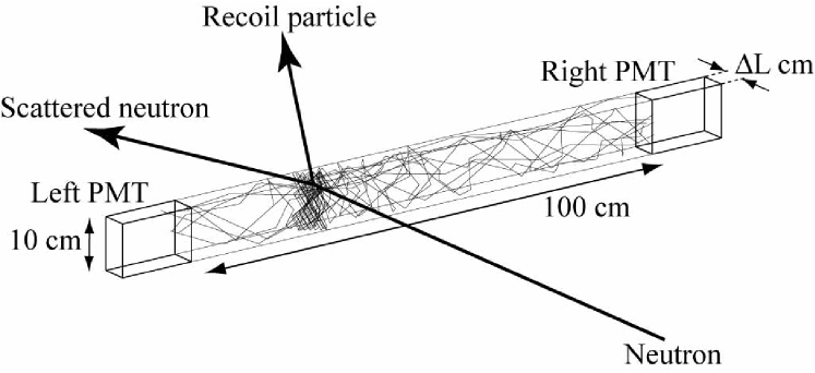
Figure 1: Illustration of the Monte-Carlo simulation with geant4. The neutron beam with $T_{n}$ = 200 or 300 MeV bombard a plastic scintillator with a size of 100 cm $\times$ 10 cm $\times$ $\Delta L$ cm. The optical photons generated by recoiled charge particles propagate in the scintillator and are detected by PMTs at both ends. The time information, $t_{L}$ and $t_{R}$, deduced from PMT signals are used to evaluate the time of flight $t$ and its width $\Delta t$.

We performed the Monte-Carlo simulation in order to describe the energy resolution $T_{n}$ quantitatively as a function of $\Delta L$. The computer library geant4 [23] was used to simulate the neutron-induced reactions in scintillator material, the generation of optical photons, and their propagation. The scintillator material is assumed to be the plastic scintillator Saint-Gobain [24] Bicron BC408 with a hydrogen to carbon ratio of H/C = 1.1. The size of the scintillator is 100 cm $\times$ 10 cm $\times$ $\Delta L$ cm, and its configuration is the one-dimensional position-sensitive detector (hodoscope) with a thickness of $\Delta L$ cm (see Fig. 1). The length of 100 cm is same as that of the NPOL2, and the width is fixed to be 10 cm. At both ends (L:left and R:right) of the scintillator, the timing information of arrived optical photons is accumulated. The neutron flight time $t$ can be deduced by using timing information, $t_{L}$ and $t_{R}$, at both ends as

$$t=\frac{t_{L}+t_{R}}{2}-t_{\mathrm{RF}},$$ (3)

where $t_{\rm RF}$ corresponds to the timing information for an accelerator RF signal in the experiment. In practice, photo-multiplier tubes (PMTs) are mounted at both ends and optical photons are converted to electric signals. Each anode signal from PMT is fed to a constant fraction discriminator (CFD) to create a fast logic timing signal. We simulated the operation of the CFD. The upper panel of Fig. 2 is the pulse-height spectrum generated by our simulation, and the lower panel is the simulated CFD timing spectrum. The timing information is determined from the zero-crossing point of the CFD spectrum. Thus the resulting $t_{L}$ and $t_{R}$ are almost independent of an arbitrarily set discrimination level of the CFD. The time spread of the zero-crossing points in Fig. 2 corresponds to the counter-thickness ($\Delta L$) effect to $\Delta t$.

Figure 3 represents the expected energy resolutions $\Delta T_{n}$ evaluated from the simulation results as a function of $\Delta L$. The filled circles and the filled boxes correspond to the results for the measurement at $T_{n}$ = 200 and 300 MeV, respectively. In the simulation, the flight path length $L$ is 100 m and the time spread of the proton beam is assumed to be 200 ps FWHM which is a typical value of the beam from the RCNP Ring cyclotron. The $\Delta T_{n}$ values clearly depend on $\Delta L$ for both $T_{n}$ = 200 and 300 MeV. It is found that the counter thickness $\Delta L$ should be thinner than 5 cm in order to achieve the required final resolution of $\sim$500 keV at $T_{n}$ = 300 MeV. Thus we have employed the hodoscope counters with a thickness of 5cm in the NPOL3.

2.3 Comparison with experimental results

We have constructed the one-dimensional plastic scintillation counters with a size of 100 cm $\times$ 10 cm $\times$ 5cm. With these counters, we measured the ${}^{12}{\rm C}(p,n)$ reaction at $\theta_{\mathrm{lab}}$ = $0^{\circ}$ and incident beam energies of $T_{p}$ = 198 and 295 MeV. The target thickness is 38 $\mathrm{mg/cm^{2}}$ whose contribution to the final energy resolution is negligible small. The results are shown in Fig. 5. The energy resolutions were evaluated by fitting the peak of the ${}^{12}{\rm N}$ state to the standard hyper-Gaussian and they are about 280 and 500 keV FWHM for $T_{p}$ = 198 and 295 MeV data, respectively. These energy resolutions are consistent with the simulation results shown in Fig. 3, and they satisfy our requirements. These counters have been used in the NPOL3 which will discussed in the next section.

3 Neutron detector NPOL3 and its performance

3.1 Neutron detector NPOL3

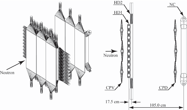
Figure 4: Schematic (left) and top (right) views of the NPOL3 system. In the polarimetry mode of NPOL3, HD1 and HD2 are the analyzer planes while NC is the catcher plane. Thin plastic scintillator planes are used to veto (CPV) or identify (CPD) charged particles.

The neutron detector NPOL3 has two main neutron detector planes, HD1 and HD2. Each plane consists of 10 stacked 100 cm $\times$ 10 cm $\times$ 5cm plastic scintillator bars made of Bicron BC408. Two thin plastic scintillator planes CPV and CPD, used to identify charged particles, complete the NPOL3 which is schematically shown in Fig. 4. Additional two-dimensional neutron counter NC is used in polarimetry mode, which will be discussed in Sec. 4. A scintillator in HD1 or HD2 is viewed by the fast Hamamatsu [25] H2431 (HD1) or H1949 (HD2) PMTs attached at each end. The one-dimensional position is deduced from the fast timing information derived from PMT. The CPV and CPD are made of three sets of plastic scintillators (BC408) with a size of 102 cm $\times$ 35 cm $\times$ 0.5 cm. The scintillator is viewed from both sides (U:up and D:down) by the Hamamatsu H7195 PMT through fish-tail shape light guides. The CPV is used to veto charged particles entered into the NPOL3, and the CPD is used to detect the recoiled charged particles.

In the neutron detector mode of NPOL3, a neutron is detected by either neutron detector plane HD1 or HD2. Furthermore we have required that the recoiled charged particle should be detected by the following detector plane. This means that we measure neutrons in the polarimetry (double-scattering) mode of the NPOL3 system. This procedure has been applied in the data analysis of the INPOL system [26], and it is useful to improve the final energy resolution as well as to reduce the low-energy tail component. Thus we have applied this procedure in our data analysis.

3.2 Light output calibration

The neutron detection efficiency depends on the threshold level $\mathcal{L}_{\mathrm{th}}$ of the scintillator light output. The total light output $\overline{\mathcal{L}}$ is constructed by taking the geometric mean of the PMT outputs at both ends, $\mathcal{L}_{L}$ and $\mathcal{L}_{R}$, as

$$\overline{\mathcal{L}}=\sqrt{\mathcal{L}_{L}\cdot\mathcal{L}_{R}}.$$ (4)

The light output $\overline{\mathcal{L}}$ is calibrated by using 4.4 MeV $\gamma$-rays from a ${}^{241}{\rm Am}$-${}^{9}{\rm Be}$ neutron source and cosmic rays (mostly $\mu^{\pm}$). In the cosmic-ray measurement, 10-bar hits in either HD1 or HD2 were required. Thus horizontal and zenith angles can be measured in HD1 and HD2, respectively, on the assumption that cosmic rays pass in straight lines through the detector plane. The $\overline{\mathcal{L}}$ for cosmic rays has been corrected for these angles in order to evaluate the $\overline{\mathcal{L}}$ in case cosmic rays pass the scintillator of 10 cm in thickness.

The left and right panels of Fig. 6 show the $\overline{\mathcal{L}}$ spectra for 4.4 MeV $\gamma$-rays and cosmic rays, respectively. We can clearly see the Compton edge (4.2 $\mathrm{MeV_{ee}}$) for the $\gamma$-ray spectrum and the sharp peak with a Landau tail for the cosmic-ray spectrum. The histograms represent the results of the Monte-Carlo simulations with geant4 described in Sec. 2. The simulations successfully reproduce the main components of the Compton edge and the sharp peak in $\gamma$-ray and cosmic-ray spectra, respectively. Furthermore they well describe the one-photon escape peak at $\sim$3.5 $\mathrm{MeV_{ee}}$ in the $\gamma$-ray spectrum and the Landau tail in the cosmic-ray spectrum. Note that the discrepancy between the data and the simulation result for 4.4 MeV $\gamma$-rays in the low $\overline{\mathcal{L}}$ region is due to the contributions from $\gamma$-rays other than 4.4 MeV $\gamma$-rays from the neutron source which are not taken into account in the simulations.

3.3 Neutron detection efficiency

The laboratory differential cross section $d\sigma_{\rm lab}/d\Omega$ is related to the number of measured neutrons $N_{n}$ as

$$\frac{d\sigma_{\rm lab}}{d\Omega}=\frac{N_{n}}{N_{p}\rho\Delta\Omega\epsilon Tf_{\rm live}},$$ (5)

where $N_{p}$ is the number of incident protons, $\rho$ is the target density, $\Delta\Omega$ is the solid angle, $\epsilon$ is the intrinsic neutron detection efficiency, $T$ is the transmission factor along the neutron flight path, and $f_{\rm live}$ is the experimental live time.

We measured the the product $\epsilon T$ by measuring the neutron yield from the $0^{\circ}$ ${}^{7}{\rm Li}(p,n){}^{7}{\rm Be}$(g.s. + 0.43 MeV) reaction which has a constant center of mass (c.m.) cross section of $\sigma_{\rm c.m.}(0^{\circ})$ = 27.0 $\pm$ 0.8 mb/sr at the bombarding energy range of $T_{p}$ = 80–795 MeV [27]. The measurements were performed at $T_{p}$ = 198 and 295 MeV by using the enriched ${}^{7}{\rm Li}$ target with a thickness of 54 $\mathrm{mg/cm^{2}}$. The integrated beam current $N_{p}$ was measured by using an electrically isolated graphite beam stop (Faraday cup) connected to a current integrator. The live time $f_{\rm live}$ was typically 90%.

The finally obtained neutron detection efficiencies ($\epsilon T$) are shown in Fig. 7 as a function of the light output threshold $\overline{\mathcal{L}}_{\rm th}$. The systematic uncertainty is estimated to be about 6% by taking into account of the uncertainties both of the ${}^{7}{\rm Li}(p,n)$ cross section and of the ${}^{7}{\rm Li}$ target thickness. It is found that the detection efficiencies are almost independent of the neutron kinetic energy with a value of $\sim$0.017 at $\overline{\mathcal{L}}_{\mathrm{th}}$ = 5 $\mathrm{MeV_{ee}}$.

4 Neutron polarimeter NPOL3 and calibration procedure

4.1 Neutron polarimeter NPOL3

In the polarimetry mode of NPOL3, the neutron detector planes, HD1 and HD2, serve as neutron polarization analyzers, and the following two-dimensional position-sensitive neutron counter NC acts as a catcher of doubly scattered neutrons or recoiled protons. Neutron polarization is determined from the asymmetry of the $\vec{n}+p$ events whose analyzing powers can be rigorously obtained by using the phase-shift analysis of the NN scattering. The $\vec{n}+p$ events are kinematically resolved from the other events by using time, position, and pulse-height information from both analyzer and catcher planes. Note that this kinematical selection significantly reduces the background events from the wraparound of slow neutrons from preceding beam pulses, cosmic rays, and the target gamma rays. However, the quasielastic $\vec{n}+\mathrm{C}$ reaction has an influence on the determination of the neutron polarization because its kinematical condition is similar to that of the $\vec{n}+p$ scattering. Thus we have measured the effective analyzing powers which include the contributions from both $\vec{n}+p$ and $\vec{n}+\mathrm{C}$ by using the polarized neutron beams.

4.2 Effective analyzing powers

There are two channels, $(\vec{n},n)$ and $(\vec{n},p)$, in the polarimetry mode. Doubly scattered neutrons and recoiled protons are measured by the catcher plane NC in $(\vec{n},n)$ and $(\vec{n},p)$ channels, respectively. The effective analyzing powers, $A_{y\mathrm{;eff}}^{nn}$ and $A_{y\mathrm{;eff}}^{np}$, of $(\vec{n},n)$ and $(\vec{n},p)$ channels can be determined by using the neutron beam with a known polarization $p_{N}^{\prime}$. $A_{y\mathrm{;eff}}^{nn}$ and $A_{y\mathrm{;eff}}^{np}$ are deduced by

$$A_{y;\mathrm{eff}}^{nn}=\frac{\epsilon^{nn}}{p_{N}^{\prime}},\quad A_{y;\mathrm{eff}}^{np}=\frac{\epsilon^{np}}{p_{N}^{\prime}},$$ (6)

where $\epsilon^{nn}$ and $\epsilon^{np}$ are the asymmetries measured for $(\vec{n},n)$ and $(\vec{n},p)$ channels, respectively.

4.3 Polarized neutron beams

The first source of polarized neutrons is the $0^{\circ}$ ${}^{2}{\rm H}(\vec{p},\vec{n})pp$ reaction at $T_{p}$ = 198 MeV. The $D_{LL}$ value at $T_{p}$ = 198 MeV was obtained by using the data in Ref. [28]. Because this reaction is mainly a Gamow-Teller transition, the polarization transfer coefficients $D_{ij}$ satisfy [19]

$$D_{NN}(0^{\circ})=-\frac{1+D_{LL}(0^{\circ})}{2}.$$ (7)

The neutron polarization $p_{N}^{\prime}$ is given by using $D_{NN}(0^{\circ})$ as

$$p_{N}^{\prime}=p_{N}D_{NN}(0^{\circ}),$$ (8)

where $p_{N}$ is the polarization of the incident proton beam.

The second source is the $0^{\circ}$ ${}^{6}{\rm Li}(\vec{p},\vec{n}){}^{6}{\rm Be}({\rm g.s.})$ reaction at $T_{p}$ = 198 MeV. This reaction is also a GT transition, and its $D_{NN}$ value was measured at $T_{p}$ = 200 MeV by Taddeucci [29]. The result can be used as a double-check of the calibration performed by using the neutrons from ${}^{2}{\rm H}(p,n)pp$.

The third source is the $0^{\circ}$ ${}^{12}{\rm C}(\vec{p},\vec{n}){}^{12}{\rm N}({\rm g.s.})$ reaction at $T_{p}$ = 198 MeV. The $D_{NN}(0^{\circ})$ value of this GT transition was also measured at $T_{p}$ = 200 MeV by Taddeucci [29]. Unfortunately, its uncertainty is relatively large compared with that of the ${}^{2}{\rm H}(\vec{p},\vec{n})$ or ${}^{6}{\rm Li}(\vec{p},\vec{n}){}^{6}{\rm Be}({\rm g.s.})$ reaction. Thus the final accuracy of $A_{y;\mathrm{eff}}$ is limited by the uncertainty of the neutron beam polarization originating from the uncertainty of $D_{NN}(0^{\circ})$, Therefore we have used the following method which does not require to know the $D_{ii}(0^{\circ})$ values.

The GT transition is the spin-flip and unnatural-parity transition, and its polarization transfer coefficients satisfy the relation in Eq. (7). Here we assume that two kinds of polarized proton beams are available; one has pure longitudinal polarization $p_{L}$ and the other has pure normal polarization $p_{N}$. The neutron polarizations at $0^{\circ}$ become $p_{L}^{\prime}$ = $p_{L}D_{LL}(0^{\circ})$ and $p_{N}^{\prime}$ = $p_{N}D_{NN}(0^{\circ})$ for the beam polarizations of $p_{L}$ and $p_{N}$, respectively. Then the resulting asymmetries measured by a neutron polarimeter are

$$\begin{split}\epsilon_{L}&=p_{L}^{\prime}A_{y;\mathrm{eff}}=p_{L}D_{LL}(0^{\circ})A_{y;\mathrm{eff}},\\ \epsilon_{N}&=p_{N}^{\prime}A_{y;\mathrm{eff}}=p_{N}D_{NN}(0^{\circ})A_{y;\mathrm{eff}}.\end{split}$$ (9)

By using Eqs. (7) and (9), $A_{y;\mathrm{eff}}$ can be expressed as

$$A_{y;\mathrm{eff}}=-\left(\frac{\epsilon_{L}}{p_{L}}+2\frac{\epsilon_{N}}{p_{N}}\right).$$ (10)

Thus the $A_{y;\mathrm{eff}}$ value can be obtained without knowing a priori the values of $D_{ii}(0^{\circ})$, and we have applied this technique to the ${}^{12}{\rm C}(\vec{p},\vec{n}){}^{12}{\rm N}({\rm g.s.})$ reaction.

4.4 Experimental conditions

We used a deuterated polyethylene ($\mathrm{CD_{2}}$) target with a thickness of 228 $\mathrm{mg/cm^{2}}$ as a deuteron target. Neutrons from the ${}^{2}{\rm H}(\vec{p},\vec{n})pp$ reaction were clearly separated from those from the ${}^{12}{\rm C}(\vec{p},\vec{n}X)$ reaction since the former reaction $Q$ value of $-2.2$ MeV is significantly smaller than the latter $Q$ value of $\geq$ $-18.1$ MeV. We also used 99% enriched ${}^{6}{\rm Li}$ and natural C targets with thicknesses of 181 and 38 $\mathrm{mg/cm^{2}}$, respectively. The proton beam intensity and its polarization are typically 80 nA and 0.70, respectively.

4.5 Sector methods

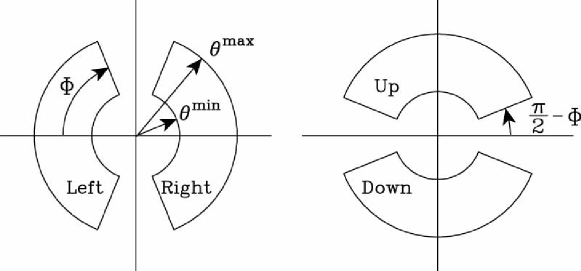
Figure 8: Illustration of the sector definition on the catcher plane NC for left/right (left panel) and up/down (right panel) asymmetries.

We have adopted the sector method in order to obtain the asymmetry. In this method, the plane $(\theta,\phi)$ defined by the scattering polar angle $\theta$ and the azimuthal angle $\phi$ is divided into four sectors: Left, Right, Up, and Down, as is shown in Fig. 8. Each sector is defined by scattering angle limits $\theta^{\mathrm{min}}$ and $\theta^{\mathrm{max}}$ and the azimuthal half-angle $\Phi$.

The asymmetry $\epsilon$ is calculated by using the event numbers in these sectors. For example, the relation between the left-right asymmetry $\epsilon_{N}^{\prime}$ and the event numbers is as follows. The azimuthal distribution of scattered particles can be described as

$$f(\phi)=\frac{1}{2\pi}(1+p_{N}^{\prime}\cos\phi),$$ (11)

where we suppress the $\theta$ dependence for simplicity. Then the event numbers scattered to left and right become

$$\begin{split}Y_{L}&=\int_{-\Phi}^{\Phi}Nf(\phi)d\phi=\frac{N}{\pi}(\Phi+\epsilon_{N^{\prime}}\sin\Phi),\\ Y_{R}&=\int_{\pi-\Phi}^{\pi+\Phi}Nf(\phi)d\phi=\frac{N}{\pi}(\Phi-\epsilon_{N^{\prime}}\sin\Phi),\end{split}$$ (12)

where $N$ is the event number accepted in the $\theta$ bin, and the $\phi$ acceptance is assumed to be constant. Thus the asymmetry $\epsilon_{N}^{\prime}$ = $p_{N}^{\prime}A_{y;\mathrm{eff}}$ is found to be

$$\epsilon_{N}^{\prime}=\frac{Y_{L}-Y_{R}}{Y_{L}+Y_{R}}\frac{\Phi}{\sin\Phi}.$$ (13)

Note that the sideway polarization $p_{S}^{\prime}$ is deduced from the up-down asymmetry $\epsilon_{S}^{\prime}$ which is obtained by substituting $L\rightarrow D$ and $R\rightarrow U$ in Eq. (13).

5 Optimization of performance of NPOL3

5.1 Optimization criteria

The performance of a polarimeter can be measured by its figure-of-merit (FOM) value defined as

$$\mathrm{FOM}=N(A_{y;\mathrm{eff}})^{2},$$ (14)

where $N$ is the total event number $Y_{L}+Y_{R}$ or $Y_{U}+Y_{D}$. We can minimize the uncertainty of the final result (neutron polarization and $D_{ij}$) by maximizing this FOM value.

We have applied three types (Types-I, II, and III) of software cuts to the measured $\theta$, $\phi$, inter-plane velocity, and pulse height information of the NPOL3. The FOM value is maximized in Type-I, whereas the $A_{y;\mathrm{eff}}$ is maximized in Type-II with keeping the FOM value larger than 40% of the optimum value. In Type-III, both FOM and $A_{y;\mathrm{eff}}$ values have been optimized with keeping the FOM value larger than 80% of the optimum value. The Type-I is the best choice from the statistical point of view in order to maximize the performance of the NPOL3. However, in general, a higher $A_{y;\mathrm{eff}}$ value in Type-II or III is helpful to reduce the systematic uncertainty of the final result. Thus we have obtained these three sets and we will select the optimum set depending on the experimental condition.

In the following, we show the results by using the data of the ${}^{2}{\rm H}(\vec{p},\vec{n})pp$ reaction because the total event number is significantly larger than that of other two polarized-neutron production reactions. The $A_{y;\mathrm{eff}}$ value is also obtained from the ${}^{6}{\rm Li}(\vec{p},\vec{n}){}^{6}{\rm Be}(g.s.)$ data by applying the same software cuts. The mean neutron energy is about 193 MeV for both the the ${}^{2}{\rm H}(\vec{p},\vec{n})pp$ and ${}^{6}{\rm Li}(\vec{p},\vec{n}){}^{6}{\rm Be}(g.s.)$ reactions. Thus we can use the results for a double check of the calibration. The same software cuts are also applied to the ${}^{12}{\rm C}(\vec{p},\vec{n}){}^{12}{\rm N}(g.s.)$ data. The mean neutron energy of $\sim$180 MeV is significantly low, therefore, the result can be used to discuss the neutron energy dependence of $A_{y;\mathrm{eff}}$.

5.2 Optimization of $\Phi$

Figure 9 shows the $A_{y;\mathrm{eff}}$ and FOM values in Type-I as a function of the azimuthal half-angle $\Phi$. The FOM values are normalized to a maximum FOM value of 1. The $A_{y;\mathrm{eff}}$ values are insensitive to the choice of $\Phi$, whereas the FOM values take a maximum at $\Phi$ $\sim$ $67^{\circ}$. This angle is consistent with the simple estimation of the optimum $\Phi$ = $66.8^{\circ}$ [21]. Because the $\Phi$ dependence is almost independent of the software cut types, we set $\Phi$ = $66.8^{\circ}$ in all cases.

5.3 Optimization of $\theta$ window

The event selection on $\theta$ is necessary to prevent dilution of $A_{y;\mathrm{eff}}$ by events with small or negative analyzing powers. Figure 10 shows the scattered-particle distribution as a function of $\theta$ in Type-I. The results in other Types-II and III are also identical. The double scattering events with a scattering angle up to $\sim$ $60^{\circ}$ are accepted by the NPOL3. The analyzing power $A_{y}(\theta)$ of the free $\vec{n}+p$ scattering is positive only up to $45^{\circ}$ and $41^{\circ}$ for $(\vec{n},n)$ and $(\vec{n},p)$ channels, respectively, at $T_{n}$ = 193 MeV. Thus part of the events should be rejected on the basis of small $A_{y}$ as described below.

Figure 11 shows the contour plots of the FOM values in Type-I as functions of both $\theta^{\mathrm{min}}$ and $\theta^{\mathrm{max}}$. Figure 12 represents the $A_{y;\mathrm{eff}}$ and FOM values as a function of either $\theta^{\mathrm{min}}$ or $\theta^{\mathrm{max}}$. In both figures, the FOM values are normalized to a maximum FOM value of 1. The FOM values strongly depend on both $\theta^{\mathrm{min}}$ and $\theta^{\mathrm{max}}$, whereas the $A_{y;\mathrm{eff}}$ values weakly depend on them except for $\theta^{\mathrm{max}}$ in the $(\vec{n},n)$ channel. In cases of Types-II and III, the optimal $(\theta^{\mathrm{min}},\theta^{\mathrm{max}})$ values are selected on basis of the criteria described in Sec. 5.1. In Table 1, we present the finally chosen $(\theta^{\mathrm{min}},\theta^{\mathrm{max}})$ values.

5.4 Optimization of $R_{v}$ window

The kinematical selection of the $\vec{n}+p$ events is performed by using the kinematical quantity $R_{v}$ defined as

$$R_{v}=\frac{v}{v_{NN}},$$ (15)

where $v$ is the measured particle velocity between the analyzer and catcher planes and $v_{NN}$ is the predicted velocity based on the NN kinematics. The $v_{NN}$ value is given by

$$v_{NN}=c\frac{2\cos\theta\sqrt{T_{n}/(T_{n}+2m_{N})}}{1-\cos^{2}\theta\,T_{n}/(T_{n}+m_{N})},$$ (16)

where $c$ is the light velocity and $m_{N}$ is the nucleon mass. Figure 13 shows the scattered-particle distribution in Type-I as a function of $R_{v}$. The peaks at $R_{v}$ $\sim$ 1 correspond to the events from the $p(\vec{n},n)p$ or $p(\vec{n},p)n$ reaction. The shoulders at $R_{v}<1$ are due to the contributions from quasielastic scattering, inelastic scattering, and wraparounds.

Figure 14 shows the contour plots of the FOM values as functions of both $R_{v}^{\mathrm{min}}$ and $R_{v}^{\mathrm{max}}$. Figure 15 represents the $A_{y;\mathrm{eff}}$ and FOM values as a function of either $R_{v}^{\mathrm{min}}$ or $R_{v}^{\mathrm{max}}$. The FOM values are normalized to a maximum FOM value of 1 in both figures. It is found that the FOM values are almost insensitive to $R_{v}^{\mathrm{max}}$ for $R_{v}^{\mathrm{max}}$ $>$ 1.3. However, $R_{v}^{\mathrm{max}}$ has been limited to be less than 1.3 to eliminated the contribution from $\gamma$-ray events with $R_{v}$ $>$ 1.5. In Types-II and III, the optimal $(R_{v}^{\mathrm{min}},R_{v}^{\mathrm{max}})$ values are selected on basis of the criteria described in Sec. 5.1. The final $(R_{v}^{\mathrm{min}},R_{v}^{\mathrm{max}})$ values chosen are listed in Table 1.

5.5 Optimization of $\overline{\mathcal{L}}_{\mathrm{th}}$

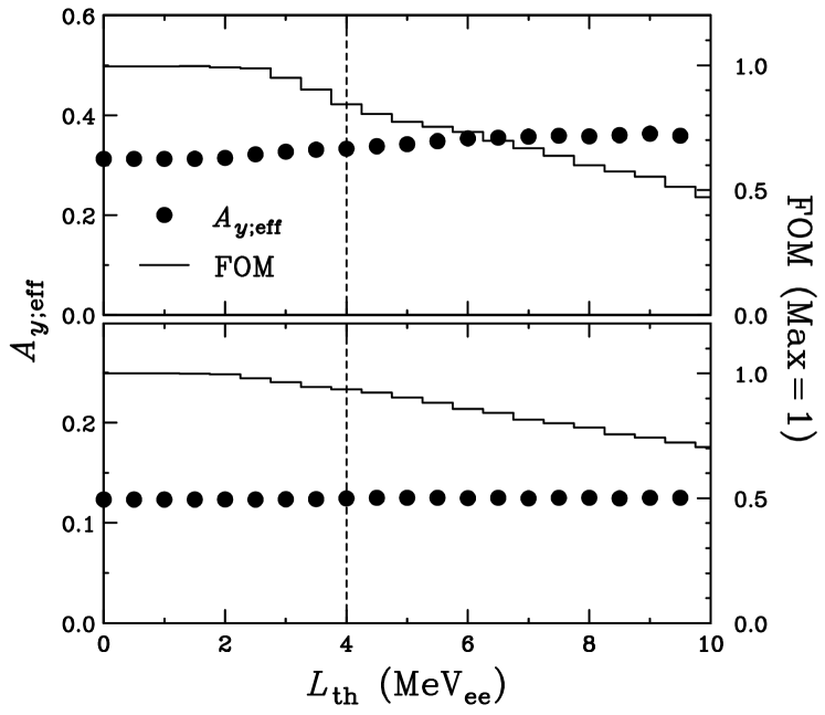
Figure 16: Effective analyzing powers $A_{y;\mathrm{eff}}$ and FOM as a function of detection threshold $\overline{\mathcal{L}}_{\mathrm{th}}$. The upper and lower panels correspond to the results for $(\vec{n},n)$ and $(\vec{n},p)$ channels, respectively.

Figure 16 shows the $A_{y;\mathrm{eff}}$ and FOM values in Type-I as a function of $\overline{\mathcal{L}}_{\mathrm{th}}$. The FOM values monotonously decrease as increasing $\overline{\mathcal{L}}_{\mathrm{th}}$, whereas the $A_{y;\mathrm{eff}}$ values are almost independent of $\overline{\mathcal{L}}_{\mathrm{th}}$. In all software cut types, we have chosen $\overline{\mathcal{L}}_{\mathrm{th}}$ = 4 $\mathrm{MeV}_{ee}$ to ensure reproducibility in the offline analysis rather than just accept the hardware threshold of $\sim$2 $\mathrm{MeV}_{ee}$.

6 Performance of polarimeter NPOL3

6.1 Effective analyzing powers

The effective analyzing powers $A_{y;\mathrm{eff}}$ obtained from the ${}^{2}{\rm H}(\vec{p},\vec{n})pp$ data by applying previously described software cuts are summarized in Table 2. The $A_{y;\mathrm{eff}}$ values deduced from the ${}^{6}{\rm Li}(\vec{p},\vec{n}){}^{6}{\rm Be}(\mathrm{g.s.})$ data are also listed in Table 2. The results of the ${}^{2}{\rm H}(\vec{p},\vec{n})pp$ and ${}^{6}{\rm Li}(\vec{p},\vec{n}){}^{6}{\rm Be}(\mathrm{g.s.})$ data are consistent with each other within their statistical uncertainties, which suggests the reliability of the present calibration procedure.

The $A_{y;\mathrm{eff}}$ values deduced from the ${}^{12}{\rm C}(\vec{p},\vec{n}){}^{12}{\rm N}(\mathrm{g.s.})$ data are plotted in Fig. 17, and they are also listed in Table 2. The results of the ${}^{2}{\rm H}(\vec{p},\vec{n})pp$ data are also displayed in Fig. 17. The $A_{y;\mathrm{eff}}$ values have been estimated as a function of $T_{n}$ on the basis of the free $\vec{n}+p$ analyzing powers derived from the NN phase shift analysis [30]. In the calculations, the $(\theta,\phi)$ cuts and the counter geometries have been properly taken into account. The solid curves in Fig. 17 show the results of the calculations. The measured $A_{y;\mathrm{eff}}$ values are different from the calculated values by factors of 0.73–0.79 and 1.16–1.29 for $(\vec{n},n)$ and $(\vec{n},p)$ channels, respectively, depending on the event cut types. The difference of $A_{y;\mathrm{eff}}$ is mainly due to the contributions from the quasielastic $\vec{n}+\mathrm{C}$ events. The dashed curves represent the calculated $A_{y;\mathrm{eff}}$ values normalized to reproduced the experimental results. These normalized values will be used in future data analysis in case there is no appropriate calibration result.

6.2 Double scattering efficiency

The double scattering efficiencies $(\epsilon_{\mathrm{D.S.}})$ of the NPOL3 were deduced from the data of the ${}^{2}{\rm H}(\vec{p},\vec{n})pp$ and ${}^{12}{\rm C}(\vec{p},\vec{n}){}^{12}{\rm N}(\mathrm{g.s.})$ reactions. The results are listed in Table 3. The $\epsilon_{\mathrm{D.S.}}$ values in both $(\vec{n},n)$ and $(\vec{n},p)$ channels are almost constant in the present neutron energy region.

7 Discussion

7.1 $\theta$ dependence of $A_{y;\mathrm{eff}}$

In the sector method, the events within $(\theta^{\mathrm{min}},\theta^{\mathrm{max}})$ are integrated in order to evaluate the $A_{y;\mathrm{eff}}$ values in the calibration. Thus the results can be considered as the mean effective analyzing powers in the range of $\theta$ = $\theta^{\mathrm{min}}$–$\theta^{\mathrm{max}}$. We deduced the $A_{y;\mathrm{eff}}$ values as a function of $\theta$ in order to check whether the $\vec{n}+p$ events are properly selected in our analysis. As a typical example, the results in Type-III are shown in Fig. 18. The solid curves display the angular distributions of $A_{y}(\theta)$ of the free $\vec{n}+p$ scattering. The measured angular distributions are very similar to those of the free $\vec{n}+p$ scattering. However the magnitudes are different mainly due to the contributions from the quasielastic $\vec{n}+\mathrm{C}$ events. The dashed curves are the results normalized to reproduce the measured values, and the normalization factors are 0.7 and 1.2 for $(\vec{n},n)$ and $(\vec{n},p)$ channels, respectively. The agreement of the angular distributions supports the proper kinematical selection of the $\vec{n}+p$ events in our analysis.

7.2 Comparison with INPOL system

Here we compare the performance of the NPOL3 system with that of the INPOL system [26] which has been used in the same energy region. For the $(\vec{n},n)$ channel, the NPOL3 has $\sim$$1/2$ volume for both analyzer and catcher planes compared with the INPOL. Thus the double scattering efficiency $\epsilon_{\mathrm{D.S}}$ and the corresponding FOM value of the NPOL3 is expected to be $\sim$$1/4$ of those of the INPOL. The FOM value of the NPOL3 is $0.28\times 10^{-4}$ in Type-I at $T_{n}$ = 193 MeV, which is about $1/4$ of that of the INPOL reported as $0.92\times 10^{-4}$ at $T_{n}$ = 194 MeV. For the $(\vec{n},p)$ channel, the FOM value of the NPOL3 is expected to be similar to that of the INPOL because their volume of the analyzer planes is similar with each other. In fact, the FOM value of $0.89\times 10^{-4}$ in Type-I is close to that of $0.81\times 10^{-4}$ of the INPOL. Thus we conclude that the performance of the NPOL3 is very similar to that of the INPOL by taking into account of the difference of the thicknesses of both analyzer and catcher planes.

8 Summary

The high resolution neutron polarimeter NPOL3 has been constructed and developed to measure polarization transfer observables $D_{ij}$ for $(\vec{p},\vec{n})$ reactions at intermediate energies around $T_{p}$ = 200 MeV. The NPOL3 system can measure the normal as well as sideways components of the neutron polarization simultaneously. The other longitudinal component can be measured by using the neutron spin rotation magnet described in Ref. [22]. Thus we can perform the measurement of a complete set of $D_{ij}$ with a high resolution of $\sim$300 keV by using the NPOL3.

The performance of the NPOL3 system was studied by using the polarized neutrons from ${}^{2}{\rm H}(p,n)pp$, ${}^{6}{\rm Li}(p,n){}^{6}{\rm Be}(\mathrm{g.s.})$, and ${}^{12}{\rm C}(p,n){}^{12}{\rm N}(\mathrm{g.s.})$ reactions at $T_{p}$ = 198 MeV. The effective analyzing powers in Type-I are 0.33 and 0.12 for $(\vec{n},n)$ and $(\vec{n},p)$ channels, respectively. The performance is comparable to that of the INPOL system at the same energy.

9 Acknowledgments

We are grateful to the RCNP Ring Cyclotron crew for their efforts in providing a good quality beam. The experiments were performed at RCNP under program numbers E218 and E236. This work was supported in part by the Grant-in-Aid for Scientific Research No. 14702005 of the Ministry of Education, Culture, Sports, Science, and Technology of Japan.

Figure 2: The pulse-height (upper panel) and CFD timing (lower panel) spectra generated by the Monte-Carlo simulation with geant4. See text for details.

Figure 3: The simulation results for the energy resolution $\Delta T_{n}$ as a function of the counter thickness $\Delta L$. The filled circles and the filled boxes represent the results for the measurement at $T_{p}$ = 200 and 300 MeV, respectively, as explained in the text.

Figure 5: Measurements of the ${}^{12}{\rm C}(p,n)$ reaction at $T_{p}$ = 198 MeV (upper panel) and 297 (lower panel) MeV with 5 cm-thick plastic scintillation counters. The curve of each panel shows the reproduction of the ${}^{12}{\rm N}(\mathrm{g.s.})$ state with the hyper-Gaussian peak.

Figure 6: Light output spectra for 4.4 MeV $\gamma$-rays from a ${}^{241}{\rm Am}$-${}^{9}{\rm Be}$ neutron source (left panel) and cosmic rays (right panel). The histograms represent the results of the Monte-Carlo simulations with geant4. See text for details.

Figure 7: Neutron detection efficiencies of 5-cm thick plastic scintillation counters as a function of detection threshold $\overline{\mathcal{L}}_{\mathrm{th}}$. The filled circles and the filled boxes represent the results at $T_{n}$ = 190 and 291 MeV, respectively.

Figure 9: Effective analyzing powers $A_{y;\mathrm{eff}}$ and FOM as a function of azimuthal half-angle $\Phi$. The upper and lower panels correspond to the results for $(\vec{n},n)$ and $(\vec{n},p)$ channels, respectively.

Figure 10: Distributions of the doubly scattered particles as a function of scattering polar angle $\theta$. The left and right panels correspond to the results for $(\vec{n},n)$ and $(\vec{n},p)$ channels, respectively.

Figure 11: FOM of NPOL3 as functions of lower and upper limits of the scattering polar angle window $(\theta^{\mathrm{min}},\theta^{\mathrm{max}})$. The left and right panels correspond to the results for $(\vec{n},n)$ and $(\vec{n},p)$ channels, respectively. The selected limits in Type-I are indicated by the filled circles.

Figure 12: Effective analyzing powers $A_{y;\mathrm{eff}}$ and FOM as a function of either lower (left panels) or upper (right panels) limit of the scattering polar angle $\theta$. The upper and lower panels correspond to the results for $(\vec{n},n)$ and $(\vec{n},p)$ channels, respectively.

Figure 13: Distributions of the doubly scattered particles as a function of velocity ratio $R_{v}$. The left and right panels correspond to the results for $(\vec{n},n)$ and $(\vec{n},p)$ channels, respectively.

Figure 14: FOM of NPOL3 as functions of lower and upper limits of the velocity ratio window $(R_{v}^{\mathrm{min}},R_{v}^{\mathrm{max}})$. The left and right panels correspond to the results for $(\vec{n},n)$ and $(\vec{n},p)$ channels, respectively. The selected limits in Type-I are indicated by the filled circles.

Figure 15: Effective analyzing powers $A_{y;\mathrm{eff}}$ and FOM as a function of either lower (left panels) or upper (right panels) limit of the velocity ratio $R_{v}$. The upper and lower panels correspond to the results for $(\vec{n},n)$ and $(\vec{n},p)$ channels, respectively.

Figure 17: Effective analyzing powers of the NPOL3 system for $(\vec{n},n)$ (filled circles) and $(\vec{n},p)$ (filled boxes) channels, respectively, as a function of neutron energy. The top, middle, and bottom panels correspond to the results in the software cut Types-I, II, and III, respectively. The solid curves represent the calculations based on the free $\vec{n}+p$ observables. The dashed curves represent the calculations normalized to reproduce the experimental data.

Figure 18: Angular distributions of effective analyzing powers of the NPOL3 system for $(\vec{n},n)$ (filled circles) and $(\vec{n},p)$ (filled boxes) channels, respectively. The solid curves represent the calculations based on the free $\vec{n}+p$ observables whereas the dashed curve represent the normalized results to reproduce the experimental data.

	Type-I		Type-II		Type-III
Quantity	FOM optimum		$A_{y;\mathrm{eff}}$ optimum		Intermediate
	$(\vec{n},n)$	$(\vec{n},p)$	$(\vec{n},n)$	$(\vec{n},p)$	$(\vec{n},n)$	$(\vec{n},p)$
$\Phi$	$67^{\circ}$	$67^{\circ}$	$67^{\circ}$	$67^{\circ}$	$67^{\circ}$	$67^{\circ}$
$\theta$	$(8^{\circ},30^{\circ})$	$(8^{\circ},53^{\circ})$	$(12^{\circ},24^{\circ})$	$(20^{\circ},53^{\circ})$	$(10^{\circ},27^{\circ})$	$(12^{\circ},53^{\circ})$
$R_{v}$	$(0.90,1.30)$	$(0.70,1.30)$	$(0.96,1.30)$	$(0.88,1.30)$	$(0.92,1.30)$	$(0.70,1.30)$
$\overline{\mathcal{L}}_{\mathrm{th}}$	$4\,\mathrm{MeV_{ee}}$	$4\,\mathrm{MeV_{ee}}$	$4\,\mathrm{MeV_{ee}}$	$4\,\mathrm{MeV_{ee}}$	$4\,\mathrm{MeV_{ee}}$	$4\,\mathrm{MeV_{ee}}$

Table 1: Optimized cuts used in the NPOL3 system.

	Type-I		Type-II		Type-III
Energy (Reaction)	FOM optimum		$A_{y;\mathrm{eff}}$ optimum		Intermediate
	$(\vec{n},n)$	$(\vec{n},p)$	$(\vec{n},n)$	$(\vec{n},p)$	$(\vec{n},n)$	$(\vec{n},p)$
193 MeV (${}^{2}{\rm H}(\vec{p},\vec{n})pp$)	0.333	0.123	0.398	0.154	0.373	0.128
	$\pm 0.008$	$\pm 0.002$	$\pm 0.013$	$\pm 0.003$	$\pm 0.009$	$\pm 0.002$
193 MeV (${}^{6}{\rm Li}(\vec{p},\vec{n}){}^{6}{\rm Be}(\mathrm{g.s.})$)	0.305	0.123	0.369	0.148	0.341	0.136
	$\pm 0.025$	$\pm 0.009$	$\pm 0.032$	$\pm 0.011$	$\pm 0.028$	$\pm 0.010$
180 MeV (${}^{12}{\rm C}(\vec{p},\vec{n}){}^{12}{\rm N}(\mathrm{g.s.})$)	0.358	0.105	0.427	0.129	0.398	0.112
	$\pm 0.021$	$\pm 0.004$	$\pm 0.034$	$\pm 0.008$	$\pm 0.024$	$\pm 0.005$

Table 2: Effective analyzing powers of the NPOL3 system.

	Type-I		Type-II		Type-III
Energy	FOM optimum		$A_{y;\mathrm{eff}}$ optimum		Intermediate
	$(\vec{n},n)$	$(\vec{n},p)$	$(\vec{n},n)$	$(\vec{n},p)$	$(\vec{n},n)$	$(\vec{n},p)$
193 MeV	$2.5\times 10^{-4}$	$5.9\times 10^{-3}$	$0.9\times 10^{-4}$	$1.7\times 10^{-3}$	$1.8\times 10^{-4}$	$4.9\times 10^{-3}$
180 MeV	$2.8\times 10^{-4}$	$6.5\times 10^{-3}$	$1.0\times 10^{-4}$	$1.8\times 10^{-3}$	$2.0\times 10^{-4}$	$5.4\times 10^{-3}$

Table 3: Double scattering efficiencies of the NPOL3 system.

References

- [1] W. M. Alberico, M. Ericson, A. Molinari, Phys. Lett. 92B (1980) 153.
- [2] W. M. Alberico, M. Ericson, A. Molinari, Nucl. Phys. A379 (1982) 429.
- [3] M. Ericson, J. Delorme, Phys. Lett. 76B (1978) 182.
- [4] H. Toki, W. Weise, Phys. Rev. Lett. 42 (1979) 1034.
- [5] J. Delorme et al., Phys. Lett. 89B (1980) 327.
- [6] C. H. Llewellyn Smith, Phys. Lett. 128B (1983) 107.
- [7] M. Ericson, A. W. Thomas, Phys. Lett. 128B (1983) 112.
- [8] B. L. Friman, V. R. Pandharipande, R. B. Wiringa, Phys. Rev. Lett. 51 (1983) 763.
- [9] E. L. Berger, F. Coester, R. B. Wiringa, Phys. Rev. D 29 (1984) 398.
- [10] D. S. Koltun, Phys. Rev. C 57 (1998) 1210.
- [11] T. N. Taddeucci et al., Phys. Rev. Lett. 73 (1994) 3516.
- [12] T. Wakasa et al., Phys. Rev. C 59 (1999) 3177.
- [13] T. Wakasa et al., Phys. Rev. C 69 (2004) 054609.
- [14] T. Wakasa, M. Ichimura, H. Sakai, nucl-ex/0411055.
- [15] E. J. Stephenson et al., Phys. Rev. Lett 78 (1997) 1636.
- [16] T. Wakasa et al, RCNP Proposal No. E236, 2004, unpublished.
- [17] K. Yako et al., nucl-ex/0411011.
- [18] T. Wakasa et al., Phys. Rev. C 55 (1997) 2909.
- [19] T. Wakasa et al., J. Phys. Soc. Jpn. 73 (2004) 1611.
- [20] H. Sakai et al, RCNP Proposal No. E218, 2003, unpublished.
- [21] T. Wakasa et al., Nucl. Instrum. Methods Phys. Res. A 404 (1998) 355.
- [22] H. Sakai et al., Nucl. Instrum. Methods Phys. Res. A 369 (1996) 120.
- [23] GEANT4 Collaboration, S. Agostinelli et al, Nucl. Instrum. Methods Phys. Res. A 506 (2003) 250.
- [24] http://www.saint-gobain.com
- [25] http://www.hpk.co.jp
- [26] M. Palarczyk et al., Nucl. Instrum. Methods Phys. Res. A 457 (2001) 309.
- [27] T. N. Taddeucci et al., Phys. Rev. C 41 (1990) 2548.
- [28] D. J. Mercer et al., Phys. Rev. Lett 71 (1993) 684.
- [29] T. N. Taddeucci, Can. J. Phys. 65 (1987) 557.
- [30] R. A. Arndt et al., computer code said (http://gwdac.phys.gwu.edu).