What’s Interesting About Strangeness Production? - An Overview of Recent Results

Abstract

In this paper I highlight a few selected topics on strange particle production in heavy-ion collisions. By studying the yield and spectra of strange particles we hope to gain understanding of the conditions reached in, and the ensuing dynamics of, the systems produced when ultra-relativistic heavy-ions are collided.

1 Motivation

The argument for studying strange particle production in heavy-ion collisions as evidence of Quark-Gluon Plasma (QGP) formation is very simple and was first suggested in 1982 [1]. The idea relies on the difference in production rates of strange particles in a hadron gas compared to strange quarks in a QGP. As there are no strange quarks in the in-coming colliding nuclei and strangeness is a conserved quantity each strange particle produced must be accompanied by a corresponding particle containing an anti-strange quark. In a hadron gas the energy threshold for strange particle production is high. The creation of a $\Lambda$ is predominantly through the reaction $\pi$ + N $\rightarrow\Lambda$ + K, with a threshold energy requirement of $\sim$530 MeV. While that of an $\overline{\Lambda}$ requires E_thresh $\sim$1420 MeV. Multi-strange particle creation not only needs a large amount of energy but is also a multi-step reaction as first a singly strange particle and then a multi-strange one must be created. Should the system convert to one whose constituents are quarks and gluons the situation simplifies. The energy threshold, for strangeness production is now reduced to $\sim$300 MeV, or twice the strange quark mass (a quark/anti-quark pair must be created). Thus strange quarks become much more abundant and upon hadronization the relative density of (multi-)strange particles is significantly enhanced over that resulting from a hadron gas. It should also be noted that in a QGP system the gluonic degrees of freedom dominate and the cross-section for gg$\rightarrow s\bar{s}$ is much larger than the cross-section for s$\bar{s}$ creation in a hadronic gas. Thus, not only is creation energetically favourable but the probability is larger. The greatest enhancement in yields is expected to be for multi-strange anti-particles such as the $\overline{\Omega}^{+}$ .

Although these arguments are old and simple they are still valid today. However, studies of strange particle production and spectra are now made to investigate many other topics relevant to heavy-ion collisions and the dynamics of the source produced.

Figure 1 highlights the important evolution sequences of a collision. The initial pre-equilibrium phase is dominated by hard scatterings, by which we mean high Q² collisions of partons. The physics of this early time is probed by high p_T particles and jet phenomenology. Much progress has been made in this area especially, through the use of strange particles to make identified hadron measurements, and it was the topic of two other sessions at this conference. Therefore, I do not cover high p_T physics in this paper.

We aim, in the early stages of the collision, to create a temperature that exceeds T_c, the critical temperature at which a transition to partonic degrees of freedom occurs. The excited region then expands and cools and drops below T_c, when hadrons re-form. It is believed that there is a large amount of re-scattering both in the partonic and hadronic phases and that the system reaches chemical equilibrium. Soon after T_c the system passes through chemical freeze-out, T_ch. At this point inelastic scatterings cease and the stable hadron ratios are frozen in. Finally kinetic freeze-out occurs when the system cools to below T_fo and elastic collisions also end. After this the particles free stream to the detectors without any further interaction.

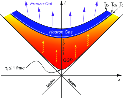
Figure 1: Schematic graph indicating the course of a heavy-ion collision, assuming the system passes through a QGP stage. See text for further details.

After first briefly, in section 2, discussing the experimental and reconstruction techniques used to identify strange particles I have organized this paper along the time-line of a collision as shown schematically in Fig. 1. In section 3, I use the strange hyperon rapidity spectra and anti-particle/particle ratios to probe how incoming protons and neutrons are transported from beam to mid-rapidity as a function of collision energy.

The issue of chemical equilibrium is discussed in section  4 and finally, section 5 describes how the p_T spectra are used to probe the source dynamics at kinetic freeze-out.

2 Techniques for Identification

Table 1 lists some of the weakly decaying strange particles, their quark content, dominant decay modes and their lifetimes. As can be seen many of these particles are either neutral or their major decay channel contains a neutral “daughter” particle, and they have lifetimes of only a few cm. Thus the majority of strange particles are identified via their decay topologies. The exception being the charged kaon, although this too is often reconstructed at higher p_T through its distinctive kink topological decay.

Particle	Quark Content	Dominant Decay Mode	Lifetime (c$\tau$)
$K^{\pm}$	($u\bar{s}$, $\bar{u}s$)	$\mu^{\pm}$ + $\nu_{\mu}$	3.7 m
$K^{0}_{s}$	($d\bar{s}$+$\bar{d}s$)	$\pi^{+}$ + $\pi^{-}$	2.7 cm
$\phi$	$s\bar{s}$	$K^{+}$ + $K^{-}$	44.6 fm
$\Lambda$	$uds$	$p$ + $\pi^{-}$	7.9 cm
$\Xi^{-}$	$dss$	$\Lambda$ + $\pi^{-}$	4.9 cm
$\Omega^{-}$	$sss$	$\Lambda$ + $K^{-}$	2.5 cm

Table 1: The major weak decaying strange particles, their quark content, dominant charged particle decay modes and lifetimes.

2.1 Topological Reconstruction

Once identified through their decay, strange particles are selected using invariant mass analysis. The decay point of the mother particle is located via the secondary vertex of the decay. The decay of the strange particles usually occurs before the tracking detectors’ active volumes, hence a visual identification of the vertex is not possible and reconstruction via combinatorial methods is employed. The decay topologies come in three distinct types and are known by the pattern they are identified via: the “V0”, the “Cascade”, and the “Kink”. These methods are described below in turn.

2.1.1 The “V0”

This pattern is produced by the decay of a neutral particle into two charged “daughters”. The neutral particle leaves no ionization trail, but upon its decay a “vee” appears in the chamber as two oppositely charged tracks apparently appear from nowhere. Reconstruction of these decay modes generally proceeds via the following process. All oppositely charged tracks are paired and projected towards the primary collision vertex. The two trajectories are compared to see if they appear to cross at a point before the primary vertex. If so these two tracks are considered candidates for a “V0” decay. The momentum components of the two charged daughters, at the now assumed decay point, are then used, assuming of the daughter particles’ masses for the decay of interest, to calculate the mother’s invariant mass using Eqn. 1. E₁ and E₂ signify the two charged daughter energies and p_x1 etc, their individual momentum components.

$$M_{invariant}=\sqrt{(E_{1}+E_{2})^{2}-p_{mother}^{2}}$$ (1)

$$p_{mother}^{2}=(p_{x1}+p_{x2})^{2}+(p_{y1}+p_{y2})^{2}+(p_{z1}+p_{z2})^{2}$$ (2)

If the identified tracks do indeed originate from the decay of the desired mother the invariant mass calculation will result in the correct mass, within the momentum resolution of the tracking detectors.

2.1.2 The “Cascade”

The “Cascade” decay is similar to the “V0” except there are now two decay vertices. Typically the mother decays first into a charged particle and a neutral one, which subsequently decays further into two charged daughters. Thus the decay creates a cascade of charged particles. The reconstruction of the “Cascade” decay occurs in a two step manner. First the decay vertex of the neutral daughter is reconstructed using the “V0” technique just described, and the mass and momentum components of the particle are determined. This neutral particle is then combined with all appropriately charged tracks for the mother’s decay mode and another secondary vertex is sought. Again the invariant mass is calculated assuming the masses and momenta of the decay products at the secondary vertex.

In a heavy-ion collision, where many charged particles are produced, these two techniques produce an enormous amount of random combinatorial background candidates which must be eliminated. This is done by applying various geometrical cuts to the each candidate. For instance, the parent should appear to be consistent with a particle being emitted from the primary collision point. The various daughter tracks should not have such trajectories. Another common requirement is that the secondary vertex occur more than a specified distance from the primary vertex. While this eliminates many true decay vertices it commonly removes more background than signal. As this cut is typically of several cm’s, it is obvious that the efficiency for strange particle reconstruction is low, of order a few percent. Nevertheless these methods are very successful at identifying clean signals as shown in the invariant mass plots for $\Lambda$ and $\Xi$ from STAR in Fig. 3 and Fig. 3.

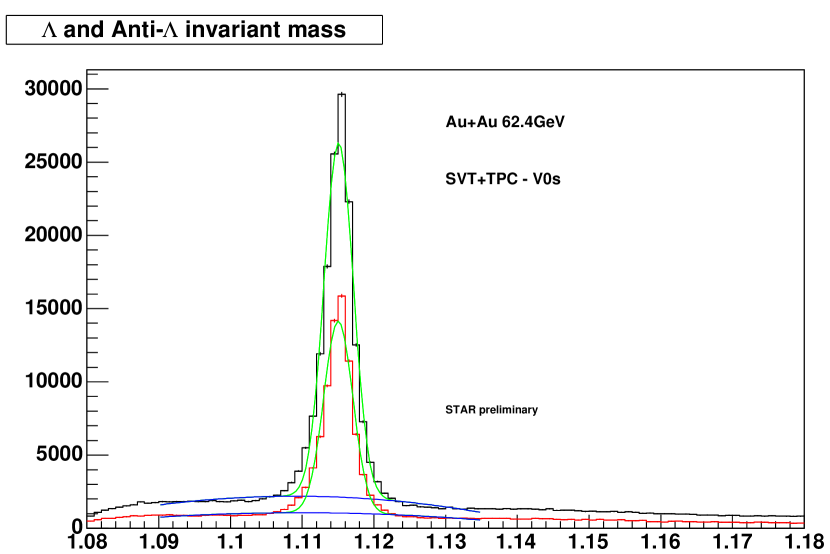
Figure 2: $\Lambda$ and $\overline{\Lambda}$ invariant mass peaks from Au+Au collisions at $\sqrt{s_{{}_{NN}}}$ = 62.4 GeV.

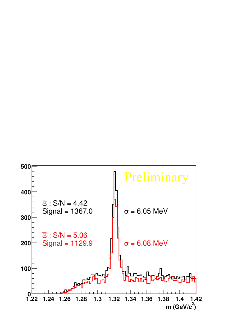
Figure 3: $\Xi^{-}$ and $\overline{\Xi}^{+}$ invariant mass peaks from Au+Au collisions at $\sqrt{s_{{}_{NN}}}$ = 200 GeV.

2.1.3 The “Kink”

The “Kink” is the result of a charged particle decaying into a stable neutral particle and a charged one. This reconstruction technique is only used when the lifetime of the parent is long and there is a high probability of the parent leaving a signal in the tracking chambers. Firstly all charged tracks appearing to emanate from the primary vertex are considered. These tracks are studied to see if their ionization paths terminate within the chamber. If such candidates are found all tracks of the same charge, whose ionization paths appear to start further away from the primary vertex than that of the now candidate parent, are considered. The two tracks are projected towards one another to see if they cross. If so this pair of tracks are considered to be a decay candidate. An invariant mass analysis is not possible with this technique as the neutral particle in the decay is not identified, hence the charged track appears to suddenly “kink” within the detector. As this technique is most commonly used to identify charged kaon decays, the main source of background is the pion decay. Kinematics force the pion to decay with a very small angle, so by insisting that the decay fall within a certain window in decay angle, and applying other geometrical cuts, the kaon can be cleanly identified.

All these techniques while having low efficiencies have an advantage over other direct particle identifications, such as dE/dx and TOF, in that they can be applied over large p_T ranges. The limit is generally the available statistics which can always be redressed through more beam time.

3 Yields and Baryon Transport

It is still a matter of debate how baryon number is carried by nucleons. It is however clear that baryon number is a conserved quantity. By colliding nuclei at high energies we can study how this baryon number becomes distributed across the whole collision region and hope to gain further insight. At top RHIC energies the beams are separated by over 10 units of rapidity. It is hard to comprehend how anything massive can be transported over such a large rapidity gap, so it was expected that the mid-rapidity region would be net-baryon free.

3.1 Net-Baryon Number at Mid-Rapidity

Fig. 4 shows the anti-baryon to baryon ratios ($\bar{p}/p$ and $\overline{\Lambda}$ /$\Lambda$) for $p+p$ and heavy-ion collisions as a function of $\sqrt{s_{{}_{NN}}}$  . It can be seen that there is a smooth transition from baryon domination at low $\sqrt{s_{{}_{NN}}}$ to a near net-baryon free region at $\sqrt{s_{{}_{NN}}}$ = 200 GeV. The new data from STAR at RHIC from Au+Au collisions as $\sqrt{s_{{}_{NN}}}$ = 62.4 GeV fits consistently into this trend.

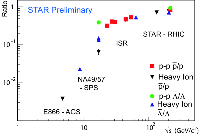
Figure 4: Anti-baryon/baryon ratios in $p+p$ and heavy-ion collisions vs. $\sqrt{s_{{}_{NN}}}$ .

In RHIC $\sqrt{s_{{}_{NN}}}$ = 200 GeV collisions $\sim$1.6 TeV appears within $-1<\eta<1$ [2], this means there is plenty of energy for the creation of strange particles. As not all of this energy is concentrated in one rapidity slice but spread over several units, it is interesting to measure not just the mid-rapidity yields but their distributions.

3.2 Rapidity Distributions

Fig. 5 shows the rapidity distributions of $\Lambda$ for four different energies at the CERN SPS [3]. It can be seen that there is a distinct evolution in shape as $\sqrt{s_{{}_{NN}}}$ increases. At $\sqrt{s_{{}_{NN}}}$ = 7.6 GeV the distribution is Gaussian, however by $\sqrt{s_{{}_{NN}}}$ = 12.3 GeV two distinct peaks, symmetric around mid-rapidity, are observed and at 17.3 GeV the distribution is approximately flat between $\pm$ 1 in rapidity. The $\Xi$ and $\Omega$ measured at 8.8 and 17.3 GeV show a less distinct change, although the Gaussian does broaden slightly in both cases. This is further evidence of baryon transport from the beams. These results and others of protons at RHIC energies [6], show clearly that on average the beam nucleons are shifted by $\sim$2 units of rapidity. At lower energies this corresponds to transportation to mid-rapidity, or near complete stopping. At higher energies this results in net baryon peaks away from mid-rapidity and a near net-baryon free region at RHIC, as shown in Fig 4.

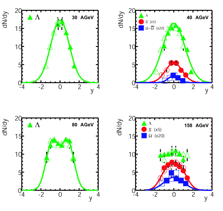
Figure 5: Energy evolution of the $\Lambda$, $\Xi$ and $\Omega$ rapidity distributions measured by NA49 at CERN SPS from $\sqrt{s_{{}_{NN}}}$ = 7.6, 8.8, 12.3, and 17.3 GeV. For clarity the $\Xi$ are scaled by a factor of 5 and the $\Omega$ by 20. The open symbols are a reflection around mid-rapidity. $\Lambda$ spectra are uncorrected for feed-down from multi-strange baryons. All spectra are preliminary except the $\Xi$ at 17.7 GeV.

It is also interesting to note that the mid-rapidity ratios are flat as a function of centrality for all collision energies suggesting that it is the collisions energy and not the number of participants, $N_{part}$, that determines the fraction of the baryon transport relative to pair production.

3.3 Mid-Rapidity Yields.

Several features can be seen in the $\sqrt{s_{{}_{NN}}}$ dependence of the strange particle yields, shown in Fig. 6. The most striking is the difference in the $\sqrt{s_{{}_{NN}}}$ dependence of the baryons and anti-baryons. This is once more a reflection of the changing net-baryon number as the collision energy increases. The anti-baryon and K${}^{0}_{s}$ yields increase smoothly as the available energy increases. The $\Lambda$ and $\Xi$ yields stay almost constant over an order of magnitude increase in energy. This is an interesting collusion of the decrease in baryon number, which causes a reduction in the yields, being counteracted by the increase in available energy.

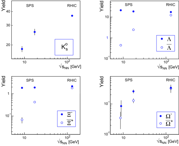
Figure 6: Mid-rapidity yields as a function of $\sqrt{s_{{}_{NN}}}$ . Data from [4] and [5].

3.4 Kaon Ratios

The quark contents of the $K^{+}$ and $K^{-}$ mesons are $\bar{s}u$ and $\bar{u}s$ respectively. Thus the $K^{-}$/$K^{+}$ ratio which effectively =$\bar{u}/u$ as $\bar{s}/s$==1, also reveals information about the systems’ baryon content, despite the Kaon being a meson. Fig. 7 shows the correlation between the $K^{-}$/$K^{+}$ and the $\bar{p}/p$ ratios for various beam energies and rapidities. As expected the two ratios show a smooth correlation, again indicating a falling net-baryon number with increasing collision energy. This correlation is well represented by the power law function $K^{-}$/$K^{+}$ = ($\bar{p}/p$)^1/4, shown as the dashed curve, rather that the function expected from a thermal interpretation with vanishing strange quark potential of $K^{-}$/$K^{+}$= ($\bar{p}/p$)^1/3, the dotted curve. This deviation might be expected as the different measurements represent different rapidity regions. However the solid curve shows the prediction from a statistical model[11] assuming T = 170 MeV and it shows good agreement. At RHIC energies the calculation show that the chemical potential, $\mu_{B}$, is $\approx$ 130 MeV at y=3 compared to $\approx$ 25 MeV at y=0. The basic premises of statistical models are described in section 4 below. The overlap of the CERN measurements, taken at mid-rapidity, to those of the BRAHMS measurements at forward rapidities should also be noted. This suggests that, chemically at least, the medium created at mid-rapidity at CERN occurs in the RHIC forward rapidities. This suggests the possibility of studying many different chemical environments by sitting at one collision energy and merely altering the rapidity region.

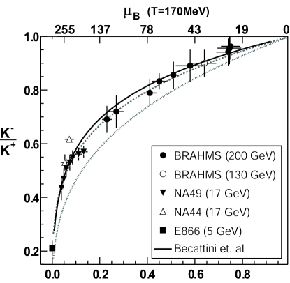
Figure 7: K^-/K⁺ ratio versus $\bar{p}$/p for various collision energies and rapidities. Data from BRAHMS [7], NA49 [8], NA44 [9] and E866 [10]. The dashed line shows K^-/K⁺ = ($\bar{p}$/p)^1/4, the dotted K^-/K⁺= ($\bar{p}$/p)^1/3 and the solid the prediction from the statistical model described in [11].

4 Chemistry

Determining the chemistry of the particles emitted from the collision region can tell us a great amount about the source created. A common way to do this is using a statistical hadronic model.

4.1 Statistical Hadronic Models

A vast amount of work has been done implementing these models to aid our understanding of heavy-ion collisions. This discussion is not intended to be exhaustive but to give an overview of the most salient points. Further details can be obtained from  [12] and references therein.

The most important features of statistical models are that they assume a thermally and chemically equilibrated system at chemical freeze-out. They make no assumptions about how the system arrived in such a state, or how long it exists in such fashion. They also assume that the system consists of non-interacting hadrons and resonances. Given these assumptions the number density of a given particle, i, with mass m_i, momentum p, energy E_i, baryon number B_i and strangeness S_i, can be calculated for a Grand Canonical ensemble where g is the spin degeneracy factor via Eqn. 3

$$N_{i}=\frac{g_{i}}{2\pi^{2}}\int_{0}^{\infty}\frac{p^{2}dp}{\exp[(E_{i}-\mu_{B}B_{i}-\mu_{s}S_{i})/(T_{ch}\pm 1)]}$$ (3)

for a given chemical freeze-out temperature, T_ch, baryo-chemical potential, $\mu_{B}$, and strangeness potential, $\mu_{s}$. The conservation laws of baryon number, strangeness and isospin have to be observed. In general these models are used to determine T_ch, $\mu_{B}$, and $\mu_{s}$ of a given data set by comparing ratios of different particles measured in the experiment to those calculated via the model. The temperature and chemical potentials are varied until a minimum in the comparison of the model to data is achieved. To obtain a good description of the data as many resonances as possible must be included. A study of Eqn. 3 shows that different particle ratios are sensitive in various degrees to T_ch, $\mu_{B}$ and $\mu_{s}$. For instance anti-baryon to baryon ratios are highly sensitive to $\mu_{B}$ but virtually insensitive to T_ch; the reverse being true of baryon to pion ratios. As the system is believed to be short lived there may not be time to fully saturate the strangeness content. What strangeness there is can be evenly distributed through the system however so the system can be thought of as in equilibrium, but the strangeness phase space will not be saturated. This non-saturation is often accounted for in the models by the factor, $\gamma_{s}$, where $\gamma_{s}$ $\leq$ 1.

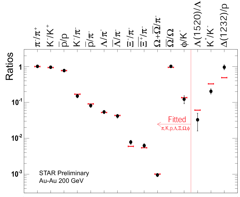
Figure 8: Measured particle ratios (symbols) and statistical model calculations (lines) [14] to the 5$\%$ most central Au+Au data at $\sqrt{s_{{}_{NN}}}$ = 200 GeV. Errors shown are systematic. The measured yields of $\pi$, K, p, $\Lambda$, $\Xi$, $\Omega$, and $\phi$ are used in the fit.

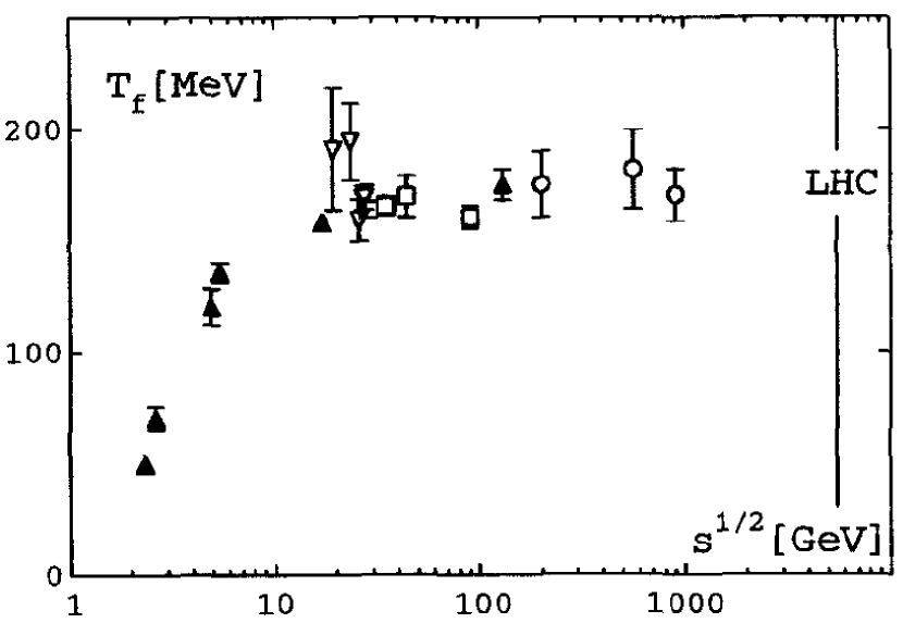
Figure 9: The calculated T_ch as a function of collision energy, for e⁺e^- (squares), pp (open triangles) $\bar{p}+p$ (circles) and A+A (closed triangles). Data from [17].

Fig. 9 shows the results of such a fit using the statistical model described in [14]. It can be seen that a good representation of the data is possible, except for the short lived resonances. A significant fraction of the particles are in resonant states at chemical freeze-out thus it is vital that they are included in thermal model descriptions despite this apparent failure to describe their yields. It is believed that the discrepancy between the calculation and measurements results from the measurable resonance yields being altered after chemical freeze-out due to re-scattering and/or regeneration in the hadronic phase. Neither re-scattering or re-generation alters the chemistry of the system they merely affect the measurable resonance signals. See [15] in these proceedings for more discussion discussion of this effect. The results of the fit give T_ch = 160 $\pm$ 5 MeV, $\mu_{B}$ = 24 $\pm$ 4 MeV, $\mu_{s}$ = 1.4 $\pm$ 1.6 MeV, and $\gamma_{s}$ = 0.99 $\pm$ 0.07. This fit suggests that the Au+Au system at RHIC is very close to complete strangeness saturation with near zero baryon and strangeness chemical potentials. Equally successful fits are obtained at lower energies and Fig. 9 shows the resulting T_ch as a function of $\sqrt{s_{{}_{NN}}}$ . There is an apparent limiting temperature reached, which is very close to the critical temperature, T_c of 170 MeV, predicted from Lattice QCD calulations[16].

It is surprising however to see that statistical models appear to work even for elementary collisions, see Fig. 9, so we should treat the results with caution. To understand how this could be possible it should be remembered that all these data sets represent the yields of particles from an event ensemble average. Therefore, it is possible that the fits do not represent true temperatures and chemical potentials but are instead the Lagrange multipliers that will result from a fit to any statistically sampled data set. These fits will only have physical meaning if each individual event can be thought of as a statistically independent system. We therefore need to establish at what collision energy, if any, state occurs and thus phase space considerations become important.

4.2 Phase Space Considerations

Statistical models utilize Grand Canonical Ensemble statistics, which is only appropriate when the system becomes large. In the Grand Canonical approach quantum numbers need only be conserved on average. Thus one can think of creating an $\Omega^{-}$ without explicitly creating, at that moment, matching particles containing 3 $\bar{s}$ quarks. Ultimately all quantum numbers have to be conserved but at each step, when the Grand Canonical limit is reached, the system can temporarily “pick up the slack”. This leads to an interesting effect upon strangeness production. In small systems, or the Canonical regime, all quantum numbers have to be conserved explicitly, this means there not only has to be energy available for strangeness creation but also the phase space. A small system therefore results in a suppression of strangeness, due to a lack of available phase space in which to create the quarks. Once the volume is sufficiently large this phase space suppression disappears and the amount of strange particle creation per unit volume becomes constant. The volume of the system is believed to be directly proportional to $N_{part}$. Although this is technically a suppression in smaller systems it is often referred to as an “enhancement” in more central A+A collisions. The “enhancement” is measured experimentally as the yield per participant relative to the yield per participant in $p+p$ (or $p+Light$ nuclei when $p+p$ is not available). Figure 11 shows the predicted behaviour for species as a function of volume, or $N_{part}$ [18]. As can be seen the larger the number of strange quarks in the particle the greater the phase space suppression effect. It has also been demonstrated that increasing the collision energy decreases the suppression of a given species.

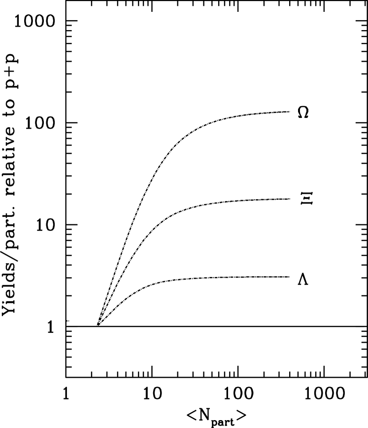
Figure 10: The calculated centrality dependence of strangeness “enhancement” for different particles in Pb+Pb collisions at $\sqrt{s_{{}_{NN}}}$ = 8.73 GeV. [18]

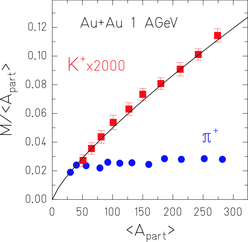
Figure 11: $K^{+}$ and $\pi^{+}$ multiplicities per participant as a function of $N_{part}$ for Au+Au collisions at $\sqrt{s_{{}_{NN}}}$ = 1 GeV[19].

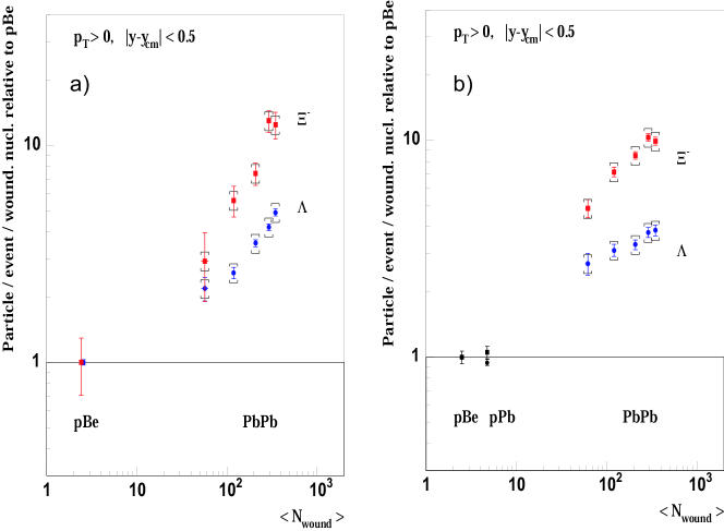
Figure 12: Hyperon enhancements as a function of number of wounded nucleons, $N_{part}$, for collisions at a) $\sqrt{s_{{}_{NN}}}$ = 8.8 GeV and b) $\sqrt{s_{{}_{NN}}}$ = 17.3 GeV as measured by the NA57 collaboration [20]. Statistical and systematic errors are shown for each data point.

At very low energies, such as those measured by the KAOS experiment at SIS, we can see the affects of canonical suppression even in the kaons[19], Fig 11. However, as the collision energy increases this kaon suppression dissipates and it has been shown that in Pb+Pb collisions of $\sqrt{s_{{}_{NN}}}$ = 17.3 GeV even the $\Lambda$ yield per participant (or wounded nucleon) appears to saturate, Fig. 12 b) [20]. There is also the suggestion of a possible saturation of the $\Xi$ yields in the most central data but the result is inconclusive. It would seem therefore that the top energy CERN collision data are showing evidence of the applicability of the Grand Canonical Ensemble for all particles up to the multi-strange baryons. The more recent $\sqrt{s_{{}_{NN}}}$ = 8.8 GeV, (Fig. 12a), however, shows enhancement factors for the $\Xi$ and $\Lambda$ that are approximately equal to the 17.3 GeV data. This result goes against our understanding of how canonical suppression is related to collision energy. Calculations have shown that the enhancement for $\Xi$ should be much higher at 8.8 than at 17.3 GeV. There are several possible explanations for this discrepancy. One could be that the assumed linear relationship between correlation volumes and $N_{part}$ is incorrect. Another is that the temperature of the source reached in the lower energy collision is not that assumed in the calculations, the enhancement factors being very sensitive to this temperature.

To try and gain further insight we turn to the RHIC measurements. Figure 14 shows the preliminary measured enhancement factors for strange hyperons from STAR. We see that for this data set the $\Lambda$ hyperons show no sign of reaching a plateau. As the SPS data appeared to saturate it is perhaps possible that the RHIC data shows an over population of strangeness in the $\Lambda$ channel. However, Figure 14, shows that the $\gamma_{s}$ factor only just reaches unity for the most central data. This indicates that the system at RHIC is only just reaching the Grand Canonical Ensemble limit for the most central collisions. So, once again, one is led to the conclusion that the correlation volume is not simply proportional to $N_{part}$. Further studies are needed to determine how the correlation volume can be mapped , if at all, onto a physically measurable quantity.

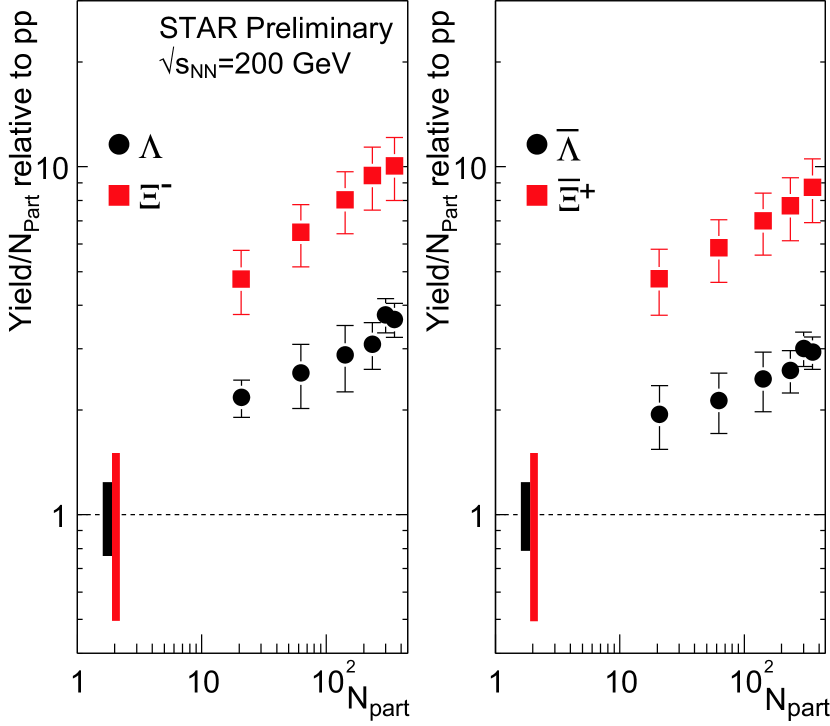
Figure 13: Enhancement factors as a function of $N_{part}$ for $\Lambda$ and $\Xi$. Error bars are statistical. The range for the $p+p$ results indicates the systematic uncertainty.

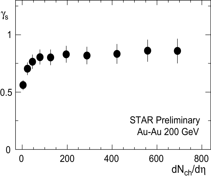
Figure 14: The $\gamma_{s}$ factor from statistical model fits of [14] as a function of the number of charged particles for Au+Au collisions at $\sqrt{s_{{}_{NN}}}$ = 200 GeV.

To conclude this section on system chemistry, we have established that for the most central Au+Au collisions at RHIC statistical models can be applied and that the resulting fits reveal physical quantities of the medium produced. It is also likely that at the top SPS energy and in the more peripheral RHIC data the models can be used but that the interpretation should be made with care.In elementary collisions and at lower energies the application of the Grand Canonical Ensemble is likely not to be correct and whilst the data can be fit by such models it is unlikely that the resulting parameters are related to physical source temperatures and chemical potentials. As stated previously, statistical models do not try to explain how the system came to be in equilibrium so the question ”How did the system arrive in this state?” remains. Microscopic hadronic models calculate that the system does not live for a sufficient amount of time to achieve equilibrium through re-scattering in the hadronic phase. An obvious mechanism is therefore to invoke a partonic phase where fast strangeness equilibration is predicted. However, a transition to a deconfined phase has not yet been confirmed.

5 Dynamics

Having established the likely properties of the source at chemical freeze-out we are next interested in its dynamical properties. The time $\Delta t$ between T_ch and T_fo, Fig. 1, can have a significant effect on the system. Elastic scatterings, while not changing the chemistry of the system, may strongly affect the momentum spectra of the particles and much of the transverse radial flow is built up during this phase. Therefore I look into the question of collective motion, I discuss only evidence for transverse radial flow as a whole session of this conference was dedicated to other types of collective motion, see [21].

5.1 m_T Scaling

Before looking for evidence for transverse radial flow in heavy ion collisions we first look at $p+p$ data from STAR. We wish to see how the m_T ( = $\sqrt{(p_{T}^{2}+m^{2})}$) spectra appear in a system where no radial flow is expected. Although we expect no collective motion in elementary collision systems there is the possibility of m_T scaling. The phenomena of m_T scaling means that the yields of all particles at a given m_T are identical. Thus the m_T spectra of all species will lie on a universal curve, ISR data have been successfully described in this manner [23]. Fig. 16 shows the m_T distributions for various particle species as measured by the STAR collaboration in $p+p$ collisions at $\sqrt{s_{{}_{NN}}}$ = 200 GeV. The spectra have been artificially normalized to obtain the agreement with a universal curve, so complete m_T scaling at 200 GeV is not observed. However, after scaling, the shape of the spectra do appear to be universal, Fig. 16. For further discussion of the $p+p$ results at $\sqrt{s_{{}_{NN}}}$ = 200 GeV see [22].

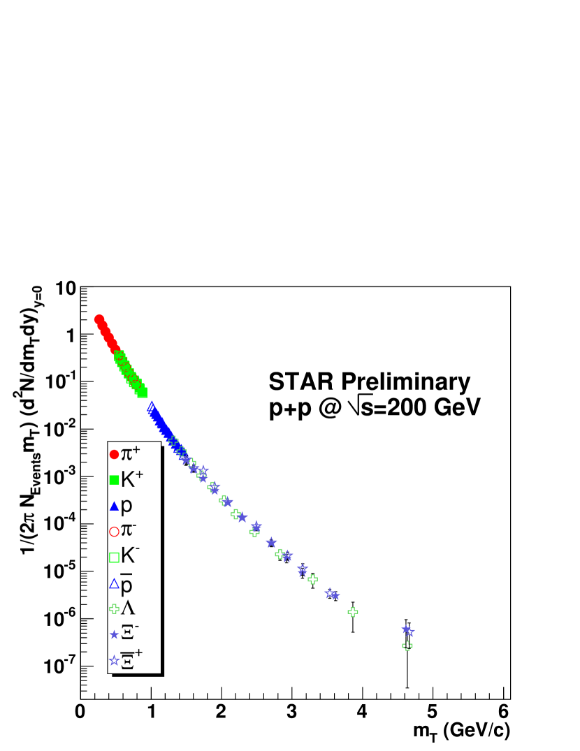
Figure 15: Preliminary $p+p$ spectra at $\sqrt{s_{{}_{NN}}}$ = 200 GeV from STAR. The data have been artificially scaled to get the best agreement with a universal curve. Errors are statistical only.

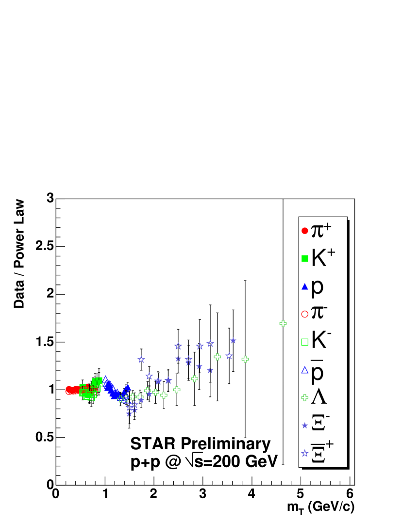
Figure 16: Ratio of data to a fit to a power law function for preliminary $p+p$ spectra from STAR after artificial scaling to get the best agreement between species.

Even such an incomplete m_T scaling is not applicable for Au+Au collisions, as is evident in Fig. 18. The Au+Au data show clear deviations for all species at low m_T, evidence for radial flow, where the push from a common flow velocity causes a depletion in all yields at low p_T.

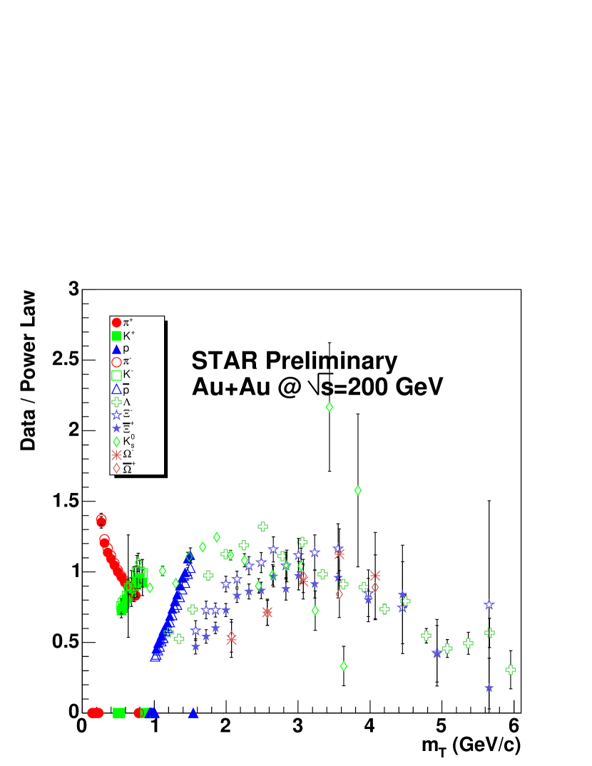
Figure 17: Ratio of data to a fit to a power law function for preliminary central Au+Au spectra from STAR after artificial scaling to get the best agreement between species.

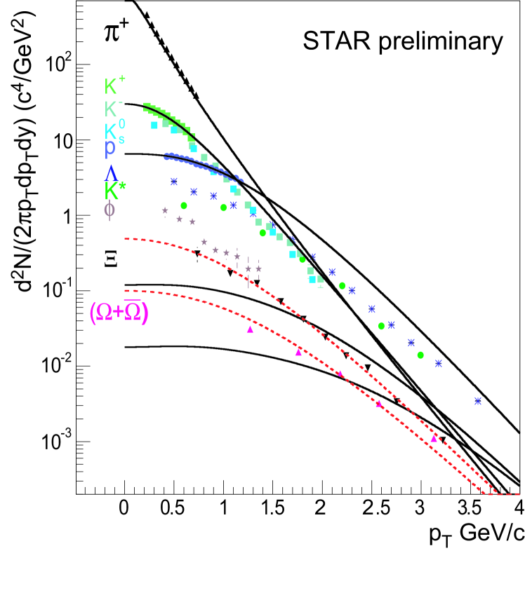
Figure 18: p_T spectra from top 5$\%$ most central Au+Au data at $\sqrt{s_{{}_{NN}}}$ = 200 GeV. Solid curves are blastwave fits to $\pi$, $K$, and $p$. The dashed curves are fits to the $\Xi$ and $\Omega$.

5.2 Transverse Radial Flow in Heavy-Ion Collisions

To extract further information about the scale of the radial flow in Au+Au collisions we try fitting a hydrodynamically inspired model, known as the “blastwave” [24]. This model assumes a common velocity profile for all particles and that they freeze-out kinetically with a common temperature, T_fo. The results of such fits can be seen in Fig. 18. A common fit to the $\pi$, $K$, and $p$ spectra yields a good representation of the data with T_fo = 89 $\pm$ 10 MeV and $<\beta>$ = 0.59 $\pm$ 0.05 c. The $\Xi$ and $\Omega$ spectra however are much steeper, indicating a hotter freeze-out temperature. Indeed when a fit is made to the $\Xi$ and $\Omega$ spectra alone, the dashed curve, T_fo = 165 MeV $\pm$ 40 MeV and $<\beta>$ = 0.45 $\pm$ 0.1 c result. This suggests that the multi-strange baryons freeze-out thermally at an earlier time than the lighter particles. At this stage the source is hotter and the radial flow is lower; it has not yet had sufficient time to build up to its final value.

The T_fo of multi-strange baryons calculated from the blastwave model is very close to that calculated by the statistical models for T_ch. This is an indication that these particles decouple almost instantly upon hadronization, but are already carring a significant radial flow. It is tempting to conclude that there is radial flow in the system before hadronization, $i.e.$ in a partonic phase.

A slightly different interpretation comes from a complete hydrodynamical simulation of the collisions [25]. In this work the authors conclude that the multi-strange baryons do not freeze-out at a significantly different time or with a different radial flow velocity. However, the key point that there is an intrinsic radial flow already , built up previous to hadronization is also one of their conclusions.

6 Summary and Conclusions

In summary I have shown that strange particle production and dynamics are key to understanding the source created in heavy-ion collisions.

The yields of strange baryons and mesons suggest a source that is in chemical equilibrium for the most central A+A collisions and that at RHIC this source displays strangeness saturation. The net-baryon number decreases smoothly with collision energy and is close to zero at RHIC. The scale of the baryon transport has a strong effect on the rapidity distributions of strange hyperons, which means that interpreting mid-rapidity yields should be done with caution. An enhancement of strange baryons per participant is observed in A+A collisions when compared to $p+p$ at the same energy. This “enhancement” is most probably due to a phase space suppression of the $p+p$ data. Obtaining such an enhancement requires a mechanism for fast saturation of the strangeness phase space which hadronic transport models cannot provide via the re-scattering of hadrons.

The dynamics of the multi-strange particles suggest a sequential freeze-out after hadronization that depends on the hadronic cross-sections. Thus the multi-strange particles appear, in a blastwave scenario, to freeze-out kinetically very close to the chemical freeze-out boundary. While this result relies on the validity of the blastwave approach both this method and a full hydrodynamical model calculate that the source created must have a sizeable radial flow during the pre-hadronic stage.

All these results, combined with those of the high p_T regime and v₂ measurements, can be taken a strong evidence of a system which, in the early phases, shows strong collective motion, is very dense and has properties consistent with partonic degrees of freedom.

References

- [1] J. Rafelski (1982) Phys. Rep. 88 331
- [2] B.B. Back et al. (PHOBOS Collaboration) nucl-ex/0410022
- [3] C. Meurer et al. (NA49 Collaboration) (2004) J. Phys. G 30 S1325
- [4] J. Adams et al. (STAR Collaboration) (2003) Phys. Lett B567 167
- [5] D. Elia et al. (NA57 Collaboration) (2004) J. Phys. G 30 S1329
- [6] I. Bearden et al. (BRAHMS Collaboration) (2004) Phys. Rev. Lett. 93 102301
- [7] I. Bearden et al. (BRAHMS Collaboration) (2003) Phys. Rev. Lett. 90 102301
- [8] Y. Afansassiev et al. (NA49 Collaboration) nucl-ex/02050002; J. Bachler et al. (1999) Nucl. Phys. A661 45
- [9] I.G. Bearden et al. (NA44 Collaboration) (1997) J.Phys. G, 23 1865,
- [10] L. Ahle et al. (E866 Collaboration) (1999) Phys. Rev. Lett. 81 2650 (1998) and Phys. Rev. C60 044904
- [11] F. Becattini et al., (2001) Phys. Rev. C64 024901
- [12] A. Bialas, (2003) Nucl. Phys. A715 95c, J. Rafelski and J. Letessier,(2003) Nucl. Phys. A715 97c , V. Koch (2003) Nucl. Phys. A715 108c
- [13] Z. Xu, (2004) J. Phys. G 30 S927
- [14] P. Braun-Munzinger, I. Heppe and J. Stachel, (1999) Phys. Lett. B465, 15
- [15] C. Markert, overview, ”What can we learn from resonance production?” These proceedings.
- [16] F. Karsch, (2002) Nucl. Phys. A698 199c
- [17] H. Satz, (2003) Nucl. Phys. A715 3c
- [18] A. Tounsi, A. Mischke and K. Redlich, (2003) Nucl. Phys. A715 565
- [19] H. Oeschler J. Cleymans and K. Redlich nucl-ex/0112005
- [20] G.E. Bruno et al. (NA57 Collaboration) (2004) J. Phys. G 30 S717
- [21] See papers from session one in these proceedings.
- [22] M. Heinz. et al. (STAR Collaboration) ”Strange particle production and systematics in at = 200 GeV” These procedings.
- [23] A. Dimitru et al., (1999) Phys. Lett. B446 326
- [24] E. Schnedermann, J. Sollfrank and U. Heinz, (1993) Phys. Rev. C48, 2462
- [25] P. Kolb and R. Rapp, (2003) Phys. Rev. C67 044903