Excitation functions of spin correlation parameters $A_{NN}$, $A_{SS}$, and $A_{SL}$ in elastic $\stackrel{{\scriptstyle\rightarrow}}{{p}}\stackrel{{\scriptstyle\rightarrow}}{{p}}$ scattering between 0.45 and 2.5 GeV

Abstract

Excitation functions of the spin correlation coefficients $A_{NN}(p_{lab},\theta_{c.m.})$, $A_{SS}(p_{lab},\theta_{c.m.})$, and $A_{SL}(p_{lab},\theta_{c.m.})$ have been measured with the polarized proton beam of the Cooler Synchrotron COSY and an internal polarized atomic beam target. Data were taken continuously during the acceleration for proton momenta $p_{lab}$ ranging from 1000 to 3300 MeV/c (kinetic energies $T_{lab}$ 450 - 2500 MeV) as well as for discrete momenta of 1430 MeV/c and above 1950 MeV/c covering angles $\theta_{c.m.}$ between 30^∘ and 90^∘. The data are of high internal consistency. Whereas $A_{SL}(p_{lab,}\theta_{c.m.})$ is small and without structures in the whole range, $A_{NN}$ and even more $A_{SS}$ show a pronounced energy dependence. The angular distributions for $A_{SS}$ are at variance with predictions of existing phase shift analyses at energies beyond 800 MeV. The impact of our results on phase shift solutions is discussed. The direct reconstruction of the scattering amplitudes from all available pp elastic scattering data considerably reduces the ambiguities of solutions.

I Introduction

This paper reports on the final part of a major experimental program devoted to a precision measurement of proton-proton elastic scattering by using the polarized beam of the Cooler Synchrotron COSY in conjunction with a polarized atomic beam target.

The EDDA experiment ALB97 ; ALT00 ; EDD03 has been conceived to provide highly accurate data of internal consistency for many projectile energies between 0.45 and 2.5 GeV covering an angular range in $\theta_{c.m.}$ from 30^∘ to 90^∘. For this purpose, it has been set up as internal beam experiment. Elastically scattered protons are detected in coincidence by a cylindrical multi-layered scintillator hodoscope. Data acquisition occurs during beam acceleration to measure quasi-continuous excitation functions as it was first done at SATURNE GAR85 . A highly polarized atomic hydrogen beam is used as target for fast and easy spin manipulation with magnetic guide fields to minimize systematic errors, a technique extensively applied by the PINTEX collaboration at IUCF VPR98 ; RAT98 at energies below 500 MeV.

Nucleon-nucleon (NN) interaction is a process fundamental to the understanding of the nuclear forces between free nucleons as well as in the nuclear environment. Elastic NN scattering data, condensed into energy dependent solutions of phase-shift analyses (PSA) BYS90 ; STO93 ; NAG96 ; ARN97 ; ARN00 , are used as an important ingredient in theoretical calculations modelling nuclear interactions. Below the pion production threshold at about 280 MeV elastic NN scattering is described with impressive precision MAC01 by several approaches, e.g. modern phenomenological and meson theoretical models LAC80 ; MAC87 ; STO94 ; WIR95 ; MAC01a , and more recently chiral perturbation theory BED02 .

Up to 800 MeV sufficient data exist that still allow an unambiguous determination of phase shift parameters and that are reasonably well reproduced by extended meson exchange models EYS04 . For even higher energies the number of contributing partial waves increases, and at the same time are the data more scarce and inconsistent. As an example no data are available for $A_{SS}$ between $T_{lab}=$ 792 MeV and 5 GeV. This coefficient is particularly sensitive to the spin-spin and spin-tensor parts of the NN interaction and the corresponding scattering amplitudes EDD03 . This may be one reason for the serious discrepancies between the PSA solutions of different groups ARN00 ; BYS98 in the regime $T_{lab}>$ 1.2 GeV, that could not be resolved with the (model independent) direct reconstruction of the scattering amplitudes. The final part of the EDDA experiment therefore aims at a substantial improvement of the data base on observables for the scattering of polarized protons on polarized protons.

In the first phase of the EDDA experiment, thin polypropylene $(CH_{2})_{n}$ fibers have been used in the circulating COSY beam to determine excitation functions of unpolarized differential cross sections ALB97 ; EDD04 . These data prompted a considerable modification and extension of PSA solutions up to 2.5 GeV ARN97 . In the second phase it was continued ALT00 ; EDD05 with the unpolarized COSY beam impinging on the polarized atomic beam target to access excitation functions of the analyzing power $A_{N}(p_{lab},\theta_{c.m.})$. In addition the results for $A_{N}$ are an important ingredient for a consistent analysis of the double polarized experiment presented here, because they allow to fix the overall polarization scale.

A short account of the results for the correlation coefficients of the third phase has been given in EDD03 , where their angular distributions were presented for the projectile energy 2.11 GeV. It was observed that the existing PSA solutions ARN00 ; BYS98 are in sharp contrast to the observable $A_{SS}$. The direct reconstruction of the scattering amplitudes (DRSA) with inclusion of our results helped to reduce ambiguities in the scattering amplitudes, indicating that these coefficients indeed provide additional constraints to the extraction of scattering amplitudes and phase shifts.

Here we present excitation functions $A_{NN}(p_{lab},\theta_{c.m.})$, $A_{SS}(p_{lab},\theta_{c.m.})$, and $A_{SL}(p_{lab},\theta_{c.m.})$ from measurements during the projectile beam acceleration as well as for 10 fixed energies ranging from 0.772 GeV to 2.493 GeV. They are compared to existing PSA solutions and enter into additional DRSA wherever the accumulated data base allows. Many details of the experiment and its analysis have been discussed in EDD04 ; EDD05 , to which we refer the reader for additional information. Here we concentrate on aspects of the experiment and its analysis for the double polarized $\stackrel{{\scriptstyle\rightarrow}}{{p}}\stackrel{{\scriptstyle\rightarrow}}{{p}}$ case. The paper is accordingly organized as follows: In Sec. II we give a short account of the experimental setup and the measurements performed. Sec. III deals with the background reduction and selection of valid scattering events. The data analysis is described in Sec. IV with emphasis on the determination of asymmetries, polarizations, correlation coefficients, and the minimization of their systematic errors. The results are then presented as excitation functions and angular distributions in Sec. V, followed by a DRSA for five projectile energies.

II The experiment

II.1 Detector and target setup

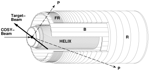
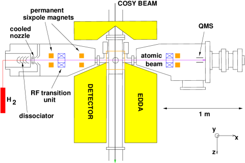
Figure 1: Scheme of the EDDA detector (top) and its combination with the atomic beam target (bottom).

The detector shown schematically in Fig. 1 consists of two cylindrical shells covering 30^∘ to 150^∘ in $\theta_{c.m.}$ for the elastic pp channel and about 85% of the full solid angle. The inner shell (HELIX) is composed of 4 layers of 160 scintillating fibers which are helically wound in opposing directions. The outer shell consists of 32 scintillator bars (B) which are running parallel to the beam axis. They are surrounded by 29 scintillator rings (R; FR), split into left and right semirings to allow independent radial readout of the scintillation light. The scintillator cross sections were designed in such a way that each particle traversing the outer layers produces a signal in two neighbouring bars and rings. Analysis of the fractional light output is used to improve the polar and azimuthal FWHM angle resolution to about 1^∘ and 1.9^∘, respectively. This geometry allows for a vertex reconstruction with a resolution of about 1 mm in the $x$-, $y$- and $z$-direction.

The polarized target EVE97 is shown in Fig. 1, too. Hydrogen atoms with nuclear polarization are prepared in an atomic beam source with dissociator, cooled nozzle, permanent sixpole magnets, and RF-transition units, where the former remove one of the two electron spin states and the latter induce a transition to a thus unpopulated hyperfine state, with only one nuclear spin state remaining. This preparation provides an atomic beam of $\sim$12 mm width (FWHM) and up to 2$\cdot 10^{11}$ $H$ atoms/cm² areal density at the intersection with the COSY beam, and a peak polarization of 90%. Details of the target performance and polarization distribution are given in EDD05 .

The direction of the target polarization in the vertex volume is defined by a magnetic guide field. Its components in the $xy$-plane are generated with two pairs of dipole magnets (A and B in Fig. 2) arranged at $z=0$ in the $xy$-plane under $\pm$45^∘ and $\pm$135^∘. Superposition of their fields of same strength yields components $\pm B_{x}$ or $\pm B_{y}$ depending on the polarities applied to the two pairs. The magnets are equipped with ferrite yokes such that field strengths in the order of 1 mT can be achieved with moderate, easily switchable currents (5 A). They exceed ambient field components by almost two orders of magnitude and thus guide the spin direction reliably. On the other hand distortions of the orbiting protons are sufficiently small; the angular kicks result in momentum dependent horizontal and vertical shifts between 20 and 50 $\mu$m. Components $\pm B_{z}$ are achieved with two solenoids mounted concentric to the COSY beam line upstream and downstream of the nominal target position.

\psfrag{Ferritjoch}{ferrite yoke}\psfrag{Targetstutzen}{flange}\psfrag{Strahlrohr}{beam pipe}\includegraphics[width=142.26378pt]{fig2.eps}

Figure 2: Magnet configuration generating the guide field in the $xy$-plane. The yoke carries 4 pole shoes that produce the field components in diagonal direction and surrounds the beam pipe. The atomic beam crosses the beam pipe horizontally.

II.2 COSY beam

$H^{-}$ ions are preaccelerated to $T_{lab}$ = 45 MeV with high nuclear polarization ($\geq$ 80%) normal to the storage orbit plane ($y$-direction) and are then stripping injected into the COSY storage ring. The protons are further accelerated with a ramping speed of 1.15 (GeV/c)/s to one of the ten flattop values $T_{ft}$ of 0.772, 1.226, 1.358, 1.546, 1.800, 1.939, 2.110, 2.301, 2.377, and 2.493 GeV with typically $3\cdot 10^{9}$ - $1.5\cdot 10^{10}$ protons circulating.

The momentary energies were derived from the RF of the cavities and the circumference of the closed orbit with uncertainties increasing from 0.25 to 2 MeV with energy. The reconstruction of beam parameters is described in EDD04 ; they vary with the momentary energy, but remain constant from cycle to cycle. COSY was tuned in a way that in vertical ($y$) direction the beam centroid and profile (6 mm FWHM) were not dependent on the momentary energy; as a consequence, the effective target polarization resulting for the overlap region with the 12 mm wide atomic beam remains constant during the ramping.

During acceleration the spins of the stored, polarized protons precess around the direction of the COSY guide fields normal to the orbit and experience depolarizing resonances. The so called imperfection resonances occur, if there is an integer number of precessions per turn such that field components in the orbit plane give rise to coherently accumulating distortions. In addition depolarization can be due to intrinsic resonances excited by horizontal field components from vertical focusing that cause betatron oscillations around the nominal orbit. At COSY, techniques have been developed LEH03 to cross both types of resonances, partly under spin flip, with a minimum of polarization loss. Figure 3 demonstrates the preservation of polarization during acceleration to the highest flattop energy as it was measured with the EDDA detector being operated as internal polarimeter LEH03 .

\psfrag{Polarisation}{polarization}\psfrag{Strahlimpuls (MeV/c)}{momentum (MeV/c)}\includegraphics[width=250.38434pt]{fig3.eps}

Figure 3: Depolarization of beam protons during acceleration across imperfection and intrinsic resonances indicated by vertical lines (the former with spin flip) to the flattop momentum of 3.3 GeV/c (kinetic energy 2.5 GeV).

II.3 Measurements

The excitation functions $A_{NN}(p_{lab},\theta_{c.m.})$, $A_{SS}(p_{lab},\theta_{c.m.})$, and $A_{SL}(p_{lab},\theta_{c.m.})$ were simultaneously measured in a sequence of acceleration cycles. Data acquisition started during ramping at 1 GeV/c (0.45 GeV) and extended over the flattop of 6 s length before the beam was decelerated to complete a COSY cycle by returning to the injection status after 13 s. Typical luminosities per cycle were 1.0 - 4.0$\cdot 10^{27}$ cm^-2s^-1. Sufficient statistics for excitation functions covering the full energy range from 0.45 GeV onward was achieved by accumulation of data in over 6$\cdot 10^{5}$ such cycles with an integrated luminosity of 12 nb^-1. The direction of the target polarization in the vertex volume was changed from cycle to cycle by switching the magnetic guide field in a sequence $+x,-x,+y,-y,+z,-z$ that was then repeated with the beam polarization flipped from $+y$ to $-y$. Such supercycles including 12 accelerator cycles were formed in order to minimize systematic errors in the extraction of the correlation coefficients (cf. Sec. IV.2) due to long term drifts of beam and/or target properties.

Measurements were performed in four running periods of up to 7 weeks length each. Each period was devoted to 2 - 4 flattop energies, with slightly varying conditions as to luminosity, cycle timing, maximum polarizations, and background conditions. Altogether 4.6$\cdot 10^{6}$ events were taken during ramping and 12.5$\cdot 10^{6}$ in the flattop time periods.

III Data Reconstruction

III.1 Selection of elastic events

The on-line triggering and off-line identification of elastic pp scattering is based on the requirement for coplanarity

$$\varphi_{1}-\varphi_{2}=180^{\circ}$$ (1)

and for kinematic correlation

$$\tan\theta_{1}\cdot\tan\theta_{2}=2\cdot\frac{m_{p}\cdot c^{2}}{(2\cdot m_{p}\cdot c^{2}+T_{lab})}$$ (2)

with $\theta_{i}$ and $\varphi_{i}$ denoting polar and azimuthal angle of the proton $i$ in the laboratory system, $m_{p}$ their mass and $T_{lab}$ the projectile proton energy. The geometry and granularity of the outer scintillator shell enables for two-prong events a fast trigger on these two requirements.

In the off-line analysis the trajectories of these correlated prongs are reconstructed from the hit and timing pattern in the inner and outer detector shell. The vertex associated with the trajectories is determined geometrically as the point of their closest approach in the target region. It is obtained with a FWHM resolution of 1.3 mm in $x$ and $y$ and 0.9 mm in $z$. The scattering angles $\theta_{i},\varphi_{i}$ are calculated with respect to this vertex position and transformed in the center-of-mass (c.m.) system assuming the kinematics of elastic pp scattering. The resulting angular resolution is 1.4^∘ in $\theta_{c.m.}$ and 1.9^∘ in $\varphi$.

Momentum conservation then requires the trajectories of elastic pp scattering to fulfill a 180^∘ correlation in the c.m. frame. The spatial angle deviation from this back-to-back scattering, furtheron referred to as kinematic deficit $\alpha$, can originate from finite angular resolution and angular straggling. It will, however, also occur for the vast majority of nonelastic background events, that can therefore be substantially suppressed with a cut on $\alpha$. The cut was optimized on data with known composition of elastic and inelastic events from our event generator ACK02 , and unpolarized EDDA-data EDD04 (using $(CH_{2})_{n}$ and carbon fiber targets), leading to a momentum dependence, viz.

$$\alpha\leq\alpha_{max}(p_{lab})=(8.32-0.72\cdot\frac{p_{lab}}{1~{}{\rm GeV/c}})^{\circ}.$$ (3)

The basic geometrical trajectory and vertex reconstruction is supplemented by a vertex fit. It improves the reconstruction within the limits of the spatial and angular resolution under the constraints of elastic scattering kinematics with intersecting trajectories. In case of convergence the $\chi^{2}_{vert}$ of this fit can be used as additional criterion for event selection.

III.2 Background reduction

Inelastic reactions and scattering involving unpolarized protons are sources of background and should be reduced or well known in the analysis. The detector is a pure hodoscope and does not allow for particle identification. Elastic events produce two sets of piercing points in both the inner and the outer detector shells. The hit pattern in the outer shell comprises two scintillator bars (B) and one semi-ring (R; FR) in each of the left and right sides. In the inner shell (HELIX) four scintillating fibers can be combined to two piercing points. Crosstalking between neighbouring channels increases the number of accepted fibers to six. The hit pattern selection reduces the amount of data by a factor of 2. Further analysis is then based on a converging vertex fit. The momentum dependent cut on the kinematic deficit, eq. (3), removes another 5% from the reconstructed events and restrains inelastic events to less than 1% in the remaining data.

Reconstructed vertices can occur far off the overlap region of projectile beam and atomic beam target, especially in the direction of the COSY beam. These events are outside the magnetic guide field region and comprise reactions with residual gas. This leads to a decreased beam polarization, which is suppressed by a cut on the $z$-vertex: -15 mm $\leq z\leq$ 20 mm. Similar effects arise in the $xy$-plane and are avoided by an elliptical cut with the axes being taken as 3 times the widths $\sigma_{x}$ and $\sigma_{y}$ of momentum dependent vertex distributions (cf. EDD04 ; EDD05 ).

After all cuts applied no more than 6% of the collected data remain for the determination of spin correlation coefficients.

IV Data analysis

IV.1 Nomenclature and coordinates

\psfrag{Beschleunigerebene}{detector plane}\psfrag{Streuebene}{scattering plane}\includegraphics[width=250.38434pt]{fig4.eps}

Figure 4: Coordinate systems: detector (laboratory) and scattering frames.

Polarization observables are described here by attaching a frame of reference to the projectile (and target) proton following the Madison convention (BYS78 , cf. Fig. 4). Its momenta $\vec{k}_{in}$ and $\vec{k}_{out}$ define the scattering plane, and $N$ is normal to it; $L$ points in the direction of $\vec{k}_{in}$, and $S$ completes the right handed frame. Using the Argonne notation BOU80 the differential cross section for scattering projectile protons of polarization $\vec{P}$ on target protons of polarization $\vec{Q}$ is then given by

$$\frac{d\sigma(\theta,\varphi)}{d\Omega}/I_{0}= 1 +A_{N}\;\;\,(P_{N}+Q_{N})$$ (4)

$$+A_{NN}\;P_{N}Q_{N}$$

$$+A_{SS}\;\,P_{S}Q_{S}$$

$$+A_{SL}(P_{S}Q_{L}+P_{L}Q_{S})$$

$$+A_{LL}\;\,P_{L}Q_{L}.$$

Here, $I_{0}=\left(\frac{d\sigma(\theta)}{d\Omega}\right)_{0}$ denotes the unpolarized differential cross section. In the experiment, $\vec{P}$ and $\vec{Q}$ are expressed in the frame $x$, $y$, $z$ that refers to the horizontal plane of the nominal projectile trajectory and the symmetry axis of the EDDA detector. It is transformed into the scattering frame with a rotation around the beam axis by the azimuthal angle $\varphi$. At present COSY provides only protons with polarization $\vec{P}=(0,P_{y},0)$ such that eq. (4) yields

$$\frac{d\sigma(\theta,\varphi)}{d\Omega}/I_{0} =1 +A_{N}\;\;\,[(P_{y}+Q_{y})\cos\varphi-Q_{x}\sin\varphi]$$ (5)

$$+A_{NN}[P_{y}Q_{y}\cos^{2}\varphi-P_{y}Q_{x}\sin\varphi\cos\varphi]$$

$$+A_{SS}\;\,[P_{y}Q_{y}\sin^{2}\varphi+P_{y}Q_{x}\sin\varphi\cos\varphi]$$

$$+A_{SL}\;\;P_{y}Q_{z}\sin\varphi.$$

The polarization observables $A_{N}$, $A_{SS}$, $A_{NN}$, and $A_{SL}$ can be deduced from the azimuthal modulation of the polarized cross section if the polarizations $P_{y},Q_{x},Q_{y}$, and $Q_{z}$ are known.

For an unpolarized beam, $\vec{P}$ = 0, and a target polarization $Q_{y}$ eq. (5) reduces to

$$\frac{d\sigma(\theta,\varphi)}{d\Omega}=I_{0}\cdot(1+A_{N}\cdot Q_{y}\cdot\cos\varphi).$$ (6)

IV.2 Determination of spin correlation coefficients

The number $N(\theta,\varphi,\vec{P},\vec{Q})$ of scattering events is related to the coefficients via

$$N(\theta,\varphi,\vec{P},\vec{Q})=\frac{d\sigma(\theta,\varphi)}{d\Omega}\cdot\Delta\Omega\cdot L(\vec{P},\vec{Q})\cdot\eta(\theta,\varphi)$$ (7)

with the integrated luminosity $L$, the detection efficiency $\eta$, and the solid angle $\Delta\Omega$ subtended by the detector element.

In ALT00 ; EDD05 the analyzing power $A_{N}$ has been obtained by calculating the azimuthal asymmetry from the numbers of events for scattering to the left $[N_{L}(\theta)]$ and the right side $[N_{R}(\theta)]$. In order to correct for false asymmetries OHL73 , measurements were performed with opposite polarizations $Q_{+y}$ and $Q_{-y}$ to determine the geometrical means $R(\theta)=\sqrt{N_{L_{-}}(\theta)N_{R_{+}}(\theta)}$ and $L(\theta)=\sqrt{N_{L_{+}}(\theta)N_{R_{-}}(\theta)}$. Starting from eq. (6), the left-right asymmetry $\epsilon_{LR}=(L(\theta)-R(\theta))/(L(\theta)+R(\theta))$ allows to calculate $A_{N}$ from

$$A_{N}\langle\cos{\varphi}\rangle=\frac{\epsilon_{LR}}{Q_{y}}$$ (8)

for identical detector segments centered around the azimuthal positions $\varphi$ and $\varphi+\pi$ and $\langle\cos{\varphi}\rangle$ being the weighted mean for a segment. Similarly, $A_{N}$ was calculated from the runs with horizontal polarization $Q_{\pm x}$, the bottom-top asymmetry $\epsilon_{BT}(\theta,\varphi)$ and the weighted mean $<\sin{\varphi}>$. Details are given in ALT00 ; EDD05 .

The coefficients $A_{NN},A_{SS}$, and $A_{SL}$ can be extracted in a similar way, however with asymmetries that constitute an extension of the formalism applied to deduce $A_{N}$. For this purpose, the azimuthal coverage of the detector is subdivided into 4 identical segments centered around $\varphi=\frac{\pi}{4},\frac{3\pi}{4},\frac{5\pi}{4}$, and $\frac{7\pi}{4}$. The respective numbers of events are denoted by $N^{n}$, with $n=1,3,5$, or $7$. They vary with the orientation of the polarizations $P_{y}$ and $Q_{i}$ ($i$ = x, y, z), which are therefore indicated as subscripts, e.g. as $N^{3}_{+-}$ in case of polarizations $+P_{y}$ and $-Q_{i}$. For each quadrant and value $i$ there are 4 numbers of events ($N^{i}_{++},N^{i}_{-+},N^{i}_{--},N^{i}_{+-}$), which yield 48 numbers of events for the 12 different polarization combinations.

Inspection of eq. (5) reveals, that each 4 out of the 16 numbers of events for a given target polarization $Q_{i}$ represent the same cross section (e.g. for $Q_{x}:N^{1}_{++},N^{3}_{-+},N^{5}_{--},N^{7}_{+-}$) and can be combined to geometrical mean values $N_{1}(Q_{x})=(N^{1}_{++}\cdot N^{3}_{-+}\cdot N^{5}_{--}\cdot N^{7}_{+-})^{\frac{1}{4}}$, $N_{2}(Q_{x})=(N^{1}_{+-}\cdot N^{3}_{--}\cdot N^{5}_{-+}\cdot N^{7}_{++})^{\frac{1}{4}}$, $N_{3}(Q_{x})=(N^{1}_{-+}\cdot N^{3}_{++}\cdot N^{5}_{+-}\cdot N^{7}_{--})^{\frac{1}{4}}$, and $N_{4}(Q_{x})=(N^{1}_{--}\cdot N^{3}_{+-}\cdot N^{5}_{++}\cdot N^{7}_{-+})^{\frac{1}{4}}$. Similar combinations are found BAU01 for $Q_{y}$ and $Q_{z}$ . This way the 16 numbers of events are reduced to 4 such mean values, which are then used to define 3 different asymmetries for each of the three target polarizations $Q_{i}$:

$$\epsilon_{1}(Q_{i}) = \frac{N_{1}(Q_{i})+N_{2}(Q_{i})-N_{3}(Q_{i})-N_{4}(Q_{i})}{N_{1}(Q_{i})+N_{2}(Q_{i})+N_{3}(Q_{i})+N_{4}(Q_{i})},$$

$$\epsilon_{2}(Q_{i}) = \frac{N_{1}(Q_{i})-N_{2}(Q_{i})+N_{3}(Q_{i})-N_{4}(Q_{i})}{N_{1}(Q_{i})+N_{2}(Q_{i})+N_{3}(Q_{i})+N_{4}(Q_{i})},$$ (9)

$$\epsilon_{3}(Q_{i}) = \frac{N_{1}(Q_{i})-N_{2}(Q_{i})-N_{3}(Q_{i})+N_{4}(Q_{i})}{N_{1}(Q_{i})+N_{2}(Q_{i})+N_{3}(Q_{i})+N_{4}(Q_{i})}.$$

Evaluation of the 9 asymmetries $\epsilon_{1}(Q_{x})$, $\dots\epsilon_{3}(Q_{z})$ with eq. (5) leads to the following expressions

$$\epsilon_{1}(Q_{x}) = P_{y}\cdot A_{N}\langle\cos{\varphi}\rangle,$$ (10)

$$\epsilon_{2}(Q_{x}) = -Q_{x}\cdot A_{N}\langle\sin{\varphi}\rangle,$$ (11)

$$\epsilon_{3}(Q_{x}) = P_{y}\cdot Q_{x}\cdot(A_{SS}-A_{NN})\langle\sin{\varphi}\cos{\varphi}\rangle,$$ (12)

$$\epsilon_{1}(Q_{y}) = P_{y}\cdot A_{N}\langle\cos{\varphi}\rangle,$$ (13)

$$\epsilon_{2}(Q_{y}) = Q_{y}\cdot A_{N}\langle\cos{\varphi}\rangle,$$ (14)

$$\epsilon_{3}(Q_{y}) = P_{y}\cdot Q_{y}\cdot(A_{SS}\langle\sin^{2}{\varphi}\rangle+A_{NN}\langle\cos^{2}{\varphi}\rangle),$$ (15)

$$\epsilon_{1}(Q_{z}) = P_{y}\cdot A_{N}\langle\cos{\varphi}\rangle,$$ (16)

$$\epsilon_{2}(Q_{z}) = 0,$$ (17)

$$\epsilon_{3}(Q_{z}) = P_{y}\cdot Q_{z}\cdot A_{SL}\langle\sin{\varphi}\rangle.$$ (18)

With the analyzing power $A_{N}$ being known from ALT00 ; EDD05 , the average value $P$ of the beam polarization $P_{y}$ is derived from eqs. (10), (13), and (16). Target polarizations $Q_{x}$ and $Q_{y}$ are obtained from eqs. (11) and (14); the average value $Q$ is used for $Q_{z}$ as well, because the polarized atomic beam is aligned with the magnetic guide field in the interaction zone, a process not correlated with the generation of polarization in the atomic beam source. The remaining eqs. (12), (15), and (18) allow then to determine $A_{NN}$, $A_{SS}$, and $A_{SL}$ from the respective asymmetries including the polarizations $P$ and $Q$.

IV.2.1 Corrections of asymmetries

Eqs. (10) - (18) are based on the assumption, that the detector efficiencies do not change between measurements with flipped polarizations and are the same for the four azimuthal segments. Changing efficiencies would lead to false asymmetries and wrong geometrical mean values. The numbers of events can be efficiency-corrected, though. The sum of all events from the possible polarization combinations comprise an unpolarized measurement with no azimuthal dependence except for efficiency differences. To correct for the efficiency the calculated expectation values of the trigonometric functions are replaced by means that apply the real numbers of events for weighting. These weighting factors were Gaussian distributed with typical standard deviations of 8% - 10%; they constitute also an additional correction of other false asymmetries.

Knowledge of the COSY beam intensity is not necessary, as long as there are no systematical differences between parallel and antiparallel beam and target polarizations, namely $\pm Q_{y}$. Integral beam intensities have been measured for all polarization combinations and have been used for correction of the numbers of events.

IV.3 Systematic errors

In a first step we have checked the analysis scheme outlined by applying it to Monte Carlo generated events. The simulation was developed for and applied to the measurement of the unpolarized ALB97 excitation functions and those of the analyzing power ALT00 ; EDD05 . It includes the detector geometry in all details, energy deposition of charged reaction products, their hadronic and electromagnetic interaction in the detector material. The event generator is described in ACK02 ; it produces the elastic part of the input in accordance with the solution FA00 of the phase shift analysis of ARN00 . Data analysis occurs with the same tools that are applied to real data. Typical polarization values $P=0.8$ and $Q=0.7$ were used to generate elastic events at $T_{lab}$ = 1546 MeV. Their analysis reproduced these polarizations ($P=0.804\pm 0.004$ and $Q=0.703\pm 0.006$) as well as the spin correlation coefficients (cf. Fig. 5) essentially within the statistical uncertainties and thus confirmed the scheme culminating in eqs. (10) - (18).

\psfrag{ass}{$A_{SS}$}\psfrag{ann}{$A_{NN}$}\psfrag{asl}{$A_{SL}$}\psfrag{theta}{$\theta_{c.m.}~{}(deg)$}\includegraphics[width=250.38434pt]{fig5.eps}

Figure 5: Correlation coefficients $A_{SS}$ (left side), $A_{NN}$ (middle), $A_{SL}$ (right) as obtained from an analysis of $12\cdot 10^{6}$ elastic events that were simulated for $T_{lab}$ = 1546 MeV, $P$ = 0.8 and $Q$ = 0.7 with an angular distribution given by the SAID solution FA00 (solid lines).

There are, however, several sources of possible systematic errors that are associated with deviations of the real polarization scenario from the simulated one, or with possible correlations of the polarizations to other quantities entering into eq. (8). Those which may have a sizeable impact on the analysis will be discussed in some detail.

IV.3.1 Misalignment of polarizations $\vec{Q}$ and $\vec{P}$

Target polarizations $\vec{Q}$ may deviate in the interaction region from the intended direction due to (i) a misalignment of the guide field $\vec{B}$ or (ii) additional external field components not sufficiently compensated. In case (i) additional polarization components are generated that change their directions together with a reversion of the guide field. In contrast, (ii) causes a constant field component not sensitive to a flip of the guide field. These two cases have therefore been studied separately BAU01 . Insertion of a main component $Q_{x}$ (or $Q_{y}$) with additional small components $\delta Q_{z}$ and $\delta Q_{y}$ (or $\delta Q_{x}$) into eq. (5) yields false asymmetries that depend for (ii) quadratically on $\delta Q$, because all first order terms cancel through the formation of geometrical mean values $N(Q)$. False asymmetries are therefore expected to be small. Monte Carlo simulations indeed show no systematic deviations within the statistical uncertainties, as can be seen in the example in Fig. 6 for the case of additional, constant components. The same results hold for components that flip with the main component, although the dependence on $\delta Q_{z}$ is in this case linear. The resulting false asymmetry, however, is proportional to $A_{SL}$ (see eq. (18)), and this coefficient is generally small compared to $A_{SS}$ and $A_{NN}$.

It remains to be shown that the deviating components of the guide field $\vec{B}$ in the interaction region are indeed sufficiently small. For this purpose, simultaneous measurements of $B_{x},B_{y}$, and $B_{z}$ have been performed with a fluxgate sensor (Bartington MAG-03MCTP). It allowed to scan $\vec{B}$ in steps of 5 mm in three dimensions with a dynamical range from $10^{-9}$ T to $10^{-3}$ T. In the vertex region permanent residual $\vec{B}$ components were observed with absolute values in the order of $10^{-5}$ T; they were compensated by offset values of the guide field coils. The main components of the guide field were typically 0.7$\cdot 10^{-3}$ T. Field gradients perpendicular to its nominal direction gave rise to additional components of up to 2$\cdot 10^{-5}$ T; they generate maximum deviations from the nominal directions of a main guide field $B_{z}$ $(B_{x},B_{y})$ of less than 3.5^∘ (1.5^∘) in the fiducial interaction volume. This is small compared to the deviations assumed for the Monte Carlo calculations. The resulting errors of $Q$ components are therefore estimated to be less than 0.2%.

\psfrag{Ass}{$A_{SS}$}\psfrag{Ann}{$A_{NN}$}\psfrag{Asl}{$A_{SL}$}\psfrag{THETACM}{$\theta_{c.m.}~{}(deg)$}\includegraphics[width=250.38434pt]{fig6.eps}

Figure 6: Deviations $\Delta A_{SS}$ (left side), $\Delta A_{NN}$ (middle), $\Delta A_{SL}$ (right) of the correlation coefficients from the values of Fig. 4 obtained with additional constant polarization components $\delta Q_{x}$ = 0.05 and $\delta Q_{y}$ = 0.05 in addition to the main component $Q$.

Deviations $\delta P$ of the absolute beam polarization may occur with revision of the polarization direction from $+P$ to $-P$ as $|\pm P|=P\pm\delta P$; they are, however, eliminated by the geometrical mean values $N(P)$ of the numbers of events in first order, such that only $(\delta P)^{2}$ terms enter into eqs. (IV.2). As a consequence, simulated deviations $\delta P$ up to absolute values $\pm$0.05 have negligible impact on correlation coefficients $A_{SS}$, $A_{NN}$, $A_{SL}$ or polarizations $P,Q$. The same result is obtained for deviations $\delta Q$. Moreover, the generation of the beam polarization and the alignment of the spins along the $x$-, $y$-, and $z$-directions are independent processes and therefore $\delta Q$ is expected to vanish. This has been confirmed in a dedicated analysis of representative experimental data with standard $\chi^{2}$ minimization techniques applied to the set of eqs. (5) for the 12 spin combinations.

IV.3.2 Further systematic errors

Sources for further systematic errors include unpolarized and inelastic background. The unpolarized background was reduced through restrictions of the accepted vertex region, as described in Sec. III.2. This of course also leads to a loss of polarized scattering events but improves the effective polarizations and results in decreased statistical uncertainties of the spin correlation coefficients. Their values are not affected.

\psfrag{D1}{$\Delta A_{NN}$}\psfrag{D2}{$\Delta A_{SS}$}\psfrag{momentum}{momentum bin}\psfrag{theta}{$\theta_{c.m.}~{}(deg)$}\includegraphics[width=250.38434pt]{fig7.eps}

Figure 7: Maximum deviations $\Delta A_{NN}(p_{lab},\theta_{c.m.})$ and $\Delta A_{SS}(p_{lab},\theta_{c.m.})$ of correlation coefficients after variation of accepted inelastic background for the momentum bins $\Delta p_{lab}=$ 61 MeV/c ranging from 1060 to 2890 MeV/c. Bins beyond 2500 MeV/c are shown in dark.

\psfrag{diff1}{$\Delta A_{NN}$}\psfrag{diff2}{$\Delta A_{SS}$}\psfrag{theta}{$\theta_{c.m.}~{}(deg)$}\psfrag{39}{\hskip 5.69046pt$2300~{}MeV/c$}\psfrag{89}{\hskip 5.69046pt$3180~{}MeV/c$}\psfrag{syst}{$\Delta_{syst}$}\psfrag{stat}{$\sigma_{stat}$}\includegraphics[width=250.38434pt]{fig8.eps}

Figure 8: Comparison of maximum deviations $\Delta A_{NN}$ and $\Delta A_{SS}$ (solid histograms) of correlation coefficients after variation of accepted inelastic background for the flattop measurements at $T_{ft}$ = 1.546 GeV ($p_{lab}$ = 2300 MeV/c) and 2.377 GeV ($p_{lab}$ = 3180 MeV/c) with statistical uncertainties $\sigma_{A_{NN}}$ and $\sigma_{A_{SS}}$ (dashed lines). The thick solid lines are polynomial fits to these maximum deviations.

The inelastic background is more problematic to access, because there are few data of differential cross sections from inelastic reactions available for Monte Carlo applications. This leads only to a rough knowledge of the fraction of numbers of inelastic events and says nothing about their spin dependent behaviour. On the other hand, the effect of the inelastic background can be estimated directly from the measurement without knowledge of its exact fraction. For this purpose the fraction of accepted inelastic events has been varied by modifying $\alpha_{max}$ in eq. (3) in small steps within reasonable limits, and the variations of the spin correlation coefficients have been deduced. These variations are highly sensitive to the covered statistics. Figure 7 shows the maximum deviations for $A_{NN}$ and $A_{SS}$ derived from the data taken during ramping. On the average they increase with $p_{lab}$ and $\theta_{c.m.}$. The same procedure was performed with the flattop data. The results in Fig. 8 for two of the flattop energies demonstrate, that the inelastic background leads to variations $\Delta A_{ij}$ of less than 0.01 - 0.06 in all three correlation coefficients, which is usually less than the statistical uncertainties. Our error estimates are based on the polynomial fit values. We conclude from the comparison of Fig. 7 with Fig. 8 that significant results can be obtained from the excitation functions below 2500 MeV/c. For higher momenta flattop data will be preferred and the excitation function data of this region is excluded from the final results.

IV.4 Consistency checks

The analyzing powers $A_{N}(p_{lab},\theta_{c.m.})$ entering into eqs. (10) - (18) are taken from the preceding stage of the EDDA experiment performed with our polarized atomic beam target and the unpolarized COSY beam ALT00 ; EDD05 . For this application they have been fitted with Legendre polynomial expansions up to $5^{th}$ order and momentum dependent coefficients. Figure 9 shows an example at medium momenta.

\psfrag{AN}{\hskip 5.69046pt$A_{N}$}\psfrag{1765}{1765~{}MeV}\psfrag{1793}{1793~{}MeV}\psfrag{theta}{$\theta_{c.m.}~{}(deg)$}\includegraphics[width=250.38434pt]{fig9.eps}

Figure 9: Angular distributions $A_{N}(\theta_{c.m.})$ (solid dots) for two projectile energies together with the polynomial best fits and the respective errors; the best fit to the right distribution is repeated as dashed line in the left one as an indication for the momentum dependence.

In principle the analyzing powers can be derived directly from the present data, too, by discarding measurements with $Q_{\pm z}$ and averaging the beam polarization $P_{\pm y}$. This has been done and some representative excitation functions are compared in Fig. 10 to those of EDD05 . The values $A_{N}$ deduced this way scatter around the statistically much more precise results of the dedicated $A_{N}$ experiment, but they do not indicate systematic deviations. A quantitative comparison of all excitation functions for $\theta_{c.m.}$ ranging in increments of 4^∘ from 32^∘ to 88^∘ yields reduced values $\chi^{2}_{red}$ between 0.71 and 1.53 with a $\chi^{2}_{red}=$ 0.93 for the whole data set. This internal consistency is important, because the precise derivation of the polarizations $P$, $Q$ is based upon it.

The four running periods (cf. Sec. II.3) contribute with comparable statistics to the excitation functions; they differ, however, in several technical aspects. Therefore they were first analyzed independently and separately for each of their flattop energies $T_{ft}$. Before merging two such subsets $j$ and $k$ to one ensemble of data, their mutual consistency has been checked with a $\chi^{2}$- test

$$\chi^{2}_{red}=\frac{1}{N-1}\sum_{i=1}^{N}\frac{(O_{i}^{(j)}-O_{i}^{(k)})^{2}}{\sigma_{j}^{2}+\sigma_{k}^{2}},$$ (19)

where $O_{i}^{(j)}(p_{lab},\theta_{c.m.})$ is a spin observable deduced from the $j^{th}$ subset, $\sigma_{j}$ its statistical error, with $i$ running over all $N$ observables common to both subsets. The resulting $\chi^{2}_{red}$ values vary between 0.96 and 2.52 and give no need to discard any of the subsets. Therefore all data were combined into one set.

In a similar way the compatibility of observables from data collected in the flattop times with those from the corresponding momentum bin of the combined excitation functions can be checked. We find $\chi^{2}_{red}<$ 1.75 in all cases. The flattop results, due to their small statistical uncertainties, therefore complement the excitation functions at high energies in a very consistent manner.

\psfrag{an}{$A_{N}$}\psfrag{3}{$\theta_{c.m.}=40^{o}$}\psfrag{8}{$\theta_{c.m.}=60^{o}$}\psfrag{13}{$\theta_{c.m.}=80^{o}$}\psfrag{p}{momentum (MeV/c)}\includegraphics[width=250.38434pt]{fig10.eps}

Figure 10: Excitation functions $A_{N}(p_{lab},\theta_{c.m.})$ as obtained from the present experiment (open symbols) and from the single polarization experiment EDD05 (solid dots). The dashed line indicates the normalization point of the latter to the reference MCN90 .

IV.5 Error summary

Estimates for the systematic errors of $A_{NN}$, $A_{SS}$, and $A_{SL}$ include the contributions from the misalignment of polarization ($\leq$ 0.01), from incomplete spin flipping ($\leq$ 0.01), and from the inelastic background ($\leq$ 0.06); they are typically smaller than the statistical uncertainties even for flattop energies, and even more so during ramping.

Normalization uncertainties of the polarizations $P\cdot Q$ arise from the statistical uncertainties of the used $A_{N}$ and of the measurement of the asymmetries (cf. eqs. 10-18). The resulting uncertainty is raised by the beam polarization during acceleration, as the target polarization remains constant. The beam polarization is treated as constant only between depolarizing resonances and leads to momentum dependent normalization uncertainties between 1.1% and 2.5% below 2500 MeV/c. Flattop measurements yield comparable normalization uncertainties ranging from 2.1% at 1430 MeV/c up to 4.5% at 3100 MeV/c (and 2.8% at 3300 MeV/c) due to a restricted statistical accuracy of the determined polarizations. Additionally the analyzing powers $A_{N}$ carry an overall absolute normalization uncertainty of 1.2% EDD05 , that spread into the polarizations $P$ and $Q$ (cf. eqs. 10, 11, 13, 14, 16) and give rise to a momentum independent normalization uncertainty of 1.7% via eqs. 12, 15, 18 of all spin correlation coefficients.

In the figures representing data of this work, only the statistical uncertainties are given as error bars. The systematic errors are listed in the data tables WWW04 . Here, only the results obtained at the flattop energies are tabulated (Table I).

V Results and discussion

V.1 Excitation functions

The results will be first presented as excitation functions. For this purpose the data taken during ramping are binned into $\Delta p_{lab}\approx$ 60 MeV/c (dependent on the position of the depolarizing resonances) and $\Delta\theta_{c.m.}=$ 5^∘ intervals, the latter centered around twelve angles $\theta_{c.m.}$ from 32.5^∘ to 87.5^∘. They are supplemented by the data taken at the ten flattop energies $T_{ft}$. A representative subset of 18 (out of 36) excitation functions is shown in Figs. 11 - 13. For comparison data from other experiments and a global phase shift solution from fall 2000 ARN00 have been included in the figures.

\psfrag{37.5}{$\theta_{c.m.}=37.5^{o}$}\psfrag{47.5}{$\theta_{c.m.}=47.5^{o}$}\psfrag{57.5}{$\theta_{c.m.}=57.5^{o}$}\psfrag{67.5}{$\theta_{c.m.}=67.5^{o}$}\psfrag{77.5}{$\theta_{c.m.}=77.5^{o}$}\psfrag{87.5}{$\theta_{c.m.}=87.5^{o}$}\psfrag{T}{$T_{lab}$ (MeV)}\psfrag{p}{$p_{lab}$ (MeV/c)}\psfrag{ramp}{\small excitation function}\psfrag{flattop}{\small fixed momentum}\psfrag{said}{\small\sc Said Fa00}\psfrag{lampf}{\small\sc Lampf}\psfrag{saturne}{\small Saturne}\psfrag{pnpi}{\small\sc Pnpi}\psfrag{sin}{\small\sc Sin}\psfrag{anl}{\small\sc Anl}\includegraphics[width=250.38434pt]{fig11.eps}

Figure 11: Excitation functions $A_{NN}(p_{lab})$ for 6 angles $\theta_{c.m.}$ together with data from the SAID database.

$A_{NN}$ is positive in the whole angular and momentum range and slowly decreasing with momentum. Our data fill gaps in the existing data base especially at intermediate energies and are otherwise in good consistency with other measurements BEL80 ; MCN81 ; BHA81 ; BYS85 ; LEH87 ; LES88 ; BAL99 ; ALL00 ; ALL01 . There are deviations from the PSA solution above $p_{lab}=2000$ MeV/c, though. Significant structures at large polar angles at small momenta are reproduced in the data as well as in the PSA solution.

\psfrag{37.5}{$\theta_{c.m.}=37.5^{o}$}\psfrag{47.5}{$\theta_{c.m.}=47.5^{o}$}\psfrag{57.5}{$\theta_{c.m.}=57.5^{o}$}\psfrag{67.5}{$\theta_{c.m.}=67.5^{o}$}\psfrag{77.5}{$\theta_{c.m.}=77.5^{o}$}\psfrag{87.5}{$\theta_{c.m.}=87.5^{o}$}\psfrag{T}{$T_{lab}$ (MeV)}\psfrag{p}{$p_{lab}$ (MeV/c)}\psfrag{ramp}{excitation function}\psfrag{flattop}{fixed momentum}\psfrag{said}{\sc Said Fa00}\psfrag{lampf}{\sc Lampf}\psfrag{sin}{\sc Sin}\includegraphics[width=250.38434pt]{fig12.eps}

Figure 12: Same as in Fig. 11 for $A_{SS}(p_{lab})$.

$A_{SS}$ is a crucial observable, as it has so far only been measured below $T_{lab}=$ 792 MeV, and for the two energies $T_{p}=$ 5.1 GeV AUE76 and 10.8 GeV AUE86 that are beyond the range of present PSA solutions. Our data are negative in the covered angle and momentum range (as are the high energy data just mentioned) and in good agreement with measurement of APR83 ; DIT84 below 792 MeV. The PSA solution is determined through other observables and becomes radically different with increasing momentum at medium angles. While the data are almost momentum independent, the PSA solution rises after a small drop and even becomes positive above $p_{lab}=$2500 MeV/c. A change of sign cannot be seen in the data at all.

\psfrag{37.5}{$\theta_{c.m.}=37.5^{o}$}\psfrag{47.5}{$\theta_{c.m.}=47.5^{o}$}\psfrag{57.5}{$\theta_{c.m.}=57.5^{o}$}\psfrag{67.5}{$\theta_{c.m.}=67.5^{o}$}\psfrag{77.5}{$\theta_{c.m.}=77.5^{o}$}\psfrag{87.5}{$\theta_{c.m.}=87.5^{o}$}\psfrag{T}{$T_{lab}$ (MeV)}\psfrag{p}{$p_{lab}$ (MeV/c)}\psfrag{ramp}{excitation function}\psfrag{flattop}{fixed momentum}\psfrag{said}{\sc Said Fa00}\psfrag{lampf}{\sc Lampf}\psfrag{saturne}{Saturne}\psfrag{sin}{\sc Sin}\psfrag{anl}{\sc Anl}\includegraphics[width=250.38434pt]{fig13.eps}

Figure 13: Same as in Fig. 11 for $A_{SL}(p_{lab})$.

The correlation coefficient $A_{SL}$ is compatible with zero over a wide range of energies and angles; only at small angles for momenta below 1400 MeV/c $A_{SL}$, i.e. the single spin flip mechanism, has some systematic influence on the scattering process. Our data are in general agreement with existing LES88 ; AUE83 ; PER88 ; FON89 ; ALL98a ; GLA92 data, they are, however, for small momenta and for the fixed momenta mostly superior in statistics.

V.2 Angular distributions

Rearrangement of the data yields angular distributions for each of the 24 momentum bins and 10 flattop energies. In Fig. 14 we present the results for $p_{ft}=$ 2572 MeV/c ($T_{ft}=$ 1.8 GeV). For $A_{NN}$, good agreement is found with the SATURNE data LEH87 ; ALL00 ; ALL01 and with the PSA solution from BYS98 for this fixed energy. The energy dependent global solution SM00 reproduces the angular dependence well, but with absolute values being about 20% above the experimental ones. The angular distributions $A_{SL}(\theta_{c.m.})$ turn out to be flat, as predicted by both phase shift solutions. However, we cannot confirm the positive values found in FON89 for small angles.

For $A_{SS}$, no data exist to compare with. The PSA solutions therefore essentially represent extrapolations beyond the energy 792 MeV; both are in striking disagreement (the agreement at 90^∘ is forced by the identity BYS78 $A_{SS}=A_{NN}-1-A_{LL}$ with experimental data being available for the right hand side). Huge discrepancies like those between the PSA solutions in Fig. 14 have been observed for the 2.1 GeV data EDD03 , too, although there the single energy solution from BYS98 shows the larger deviation from our experimental data. In ARN00 these discrepancies were attributed to differences in some partial wave solutions. They may reflect a non-uniqueness also visible in the DRSA of BYS98 . It is therefore expected that the addition of the spin correlation coefficients from this work will help to remove some of the ambiguities inherent to PSA and DRSA solutions.

\psfrag{theta}{$\theta_{c.m.}(deg)$}\psfrag{ann}{$A_{NN}$}\psfrag{ass}{$A_{SS}$}\psfrag{asl}{$A_{SL}$}\psfrag{this}{{\sc Edda}, this work}\psfrag{saturne}{\sc Saturne}\includegraphics[width=250.38434pt]{fig14.eps}

Figure 14: Angular distributions of spin correlation coefficients $A_{NN}$, $A_{SS}$, and $A_{SL}$ at $T_{lab}$ = 1.8 GeV ($p_{lab}$ = 2572 MeV/c) from this work (solid symbols) and Refs. PER88 ; FON89 ; ALL98a ; ALL00 ; ALL01 (open symbols) in comparison to phase shift predictions of SAID (SM00, solid line, Ref. ARN00 ) and Bystricky et al. (dashed line with error corridor, Ref. BYS98 ).

V.3 Direct reconstruction of scattering amplitudes

Knowledge of the scattering amplitudes uniquely defines the phase shifts and all observables of nucleon nucleon scattering. The transition matrix $T$ for elastic $\stackrel{{\scriptstyle\rightarrow}}{{p}}\stackrel{{\scriptstyle\rightarrow}}{{p}}$ scattering is fully determined by five complex amplitudes BYS78 . Using the positive and negative helicity states $\mid+\rangle$ and $\mid-\rangle$ in the c.m. frame, these helicity amplitudes are JAC59 :

$$\phi_{1}=\langle++\mid{\bf T}\mid++\rangle, \phi_{4}=\langle+-\mid{\bf T}\mid-+\rangle,$$

$$\phi_{2}=\langle++\mid{\bf T}\mid--\rangle, \phi_{5}=\langle++\mid{\bf T}\mid+-\rangle,$$ (20)

$$\phi_{3}=\langle+-\mid{\bf T}\mid+-\rangle.$$

Obviously the helicity amplitudes are directly connected to the NN-interaction with its dependence on double ($\phi_{2},\phi_{4}$), single ($\phi_{5}$), and no ($\phi_{1},\phi_{3}$) spin flip. All observables, and in particular the correlation coefficients of this paper, can be expressed by these amplitudes:

$$A_{SS}\cdot I_{0} = Re(\phi_{1}\phi_{2}^{\star}+\phi_{3}\phi_{4}^{\star}),$$ (21)

$$A_{NN}\cdot I_{0} = Re(\phi_{1}\phi_{2}^{\star}-\phi_{3}\phi_{4}^{\star})+2|\phi_{5}|^{2},$$ (22)

$$A_{SL}\cdot I_{0} = Re([\phi_{1}+\phi_{2}-\phi_{3}+\phi_{4}]\phi_{5}^{\star})$$ (23)

and can thus be related to the different kinds of spin dependence.

Elastic $\stackrel{{\scriptstyle\rightarrow}}{{p}}\stackrel{{\scriptstyle\rightarrow}}{{p}}$ scattering may occur with one of the four polarization options ($S$, $N$, $L$ or no polarization) for both the two protons in the entrance and exit channel. Basic symmetry and conservation principles of the strong interaction impose constraints such that only 25 out of 256 possible polarization observables can be linearly independent. Experimental data on at least nine of them at the same beam energy and scattering angle allow to determine the helicity amplitudes by a $\chi^{2}$-minimization, with the exception of an unobservable, global phase. Actually more than 9 observables are used for such a direct reconstruction, because not all of them are linearly independent and the impact of their uncertainties is minimized.

\psfrag{theta}{$\theta_{c.m.}~{}(deg)$}\psfrag{direkte}{direct reconstruction}\psfrag{said}{\sc Said Fa00}\psfrag{phi1}{$|\phi_{1}|$}\psfrag{ang1}{$\alpha_{1}$}\psfrag{phi2}{$|\phi_{2}|$}\psfrag{ang2}{$\alpha_{2}$}\psfrag{phi3}{$|\phi_{3}|$}\psfrag{ang3}{$\alpha_{3}$}\psfrag{phi4}{$|\phi_{4}|$}\psfrag{ang4}{$\alpha_{4}$}\psfrag{phi5}{$|\phi_{5}|$}\psfrag{ang5}{$\alpha_{5}$}\psfrag{1}{\tiny$\pi$}\psfrag{0.5}{\tiny$\pi/2$}\psfrag{-0.5}{\tiny$-\pi/2$}\psfrag{-1}{\tiny$-\pi$}\includegraphics[width=250.38434pt]{fig15.eps}

Figure 15: Direct reconstruction of scattering amplitudes at $T_{lab}=$ 1.8 GeV with (filled circles) and without (open circles) inclusion of the new EDDA data. Different solutions at one angle reflect the minimum $\chi^{2}$ ambiguities. The solutions at different angles are independent. Phases are defined in the interval $-\pi\leq\alpha_{i}<\pi$. This gives rise to spurious discontinuities e.g. for $\alpha_{4}$ and $\alpha_{5}$ at $\pm\pi$. The dotted lines give the PSA solution FA00.

The EDDA data have been added to the world data base. For narrow energy intervals at 1.3, 1.6, 1.8, 2.1, and 2.4 GeV there are now 16 or more observables available that allow a direct reconstruction over a wide angular range. Results for 2.1 GeV were reported in EDD03 ; here we emphasize the reconstructions at 1.8 GeV with up to 21 observables from LEH87 ; BAL99 ; ALL00 ; PER88 ; FON89 ; ALL98a ; BAL99a ; ALL99a ; KOB94 ; LAC89b ; LAC89a ; LAC89c ; LAC89d ; LEH88 ; PER87 , among them 11 with double and 8 with triple polarization information. Since the direct reconstruction is not a global phase shift analysis, it can easily lead to several solutions that describe the data equally well. The $\chi^{2}$ also is a measure of how the new data fits into the existing data base. Similar to the results for 2.1 GeV EDD03 and the findings in BYS98 we have obtained between one and four solutions in most cases. Best results are achieved at lower energies (1.3 - 1.8 GeV).

\psfrag{theta}{$\theta_{c.m.}~{}(deg)$}\psfrag{direkte}{direct reconstruction}\psfrag{said}{\sc Said Fa00}\psfrag{phi1}{$|\phi_{1}|$}\psfrag{ang1}{$\alpha_{1}$}\psfrag{phi2}{$|\phi_{2}|$}\psfrag{ang2}{$\alpha_{2}$}\psfrag{phi3}{$|\phi_{3}|$}\psfrag{ang3}{$\alpha_{3}$}\psfrag{phi4}{$|\phi_{4}|$}\psfrag{ang4}{$\alpha_{4}$}\psfrag{phi5}{$|\phi_{5}|$}\psfrag{ang5}{$\alpha_{5}$}\psfrag{1}{\tiny$\pi$}\psfrag{0.5}{\tiny$\pi/2$}\psfrag{-0.5}{\tiny$-\pi/2$}\psfrag{-1}{\tiny$-\pi$}\includegraphics[width=250.38434pt]{fig16.eps}

Figure 16: DRSA at $T_{lab}=$ 1.6 GeV. The symbols have the same meaning as in Fig. 15.

Figure 15 shows the scattering amplitudes for 1.8 GeV in terms of absolute values and directions in the complex plane

$$\phi_{k}=|\phi_{k}|e^{i\alpha_{k}}$$ (24)

in comparison to the Said phase shift solution FA00. Solid (open) symbols denote DRSA solutions with (without) inclusion of this work. For normalization, the amplitudes are divided by $(|\phi_{1}|^{2}+|\phi_{2}|^{2}+|\phi_{3}|^{2}+|\phi_{4}|^{2}+4|\phi_{5}|^{2})^{\frac{1}{2}}=\sqrt{2I_{0}}$. Our new data do not increase the $\chi^{2}$ values of the reconstruction. This indicates that they - and in particular $A_{SS}$ in spite of the prominent deviation of the PSA solutions - are compatible with the existing experiments and provide additional constraints on phase shifts and scattering amplitudes. Please note that the inclusion of the correlation coefficients of this work tends to concentrate the DRSA solutions on one of the two branches visible without them. The moduli $|\phi_{i}|$ of all amplitudes on the preferred branches are well described through the PSA solution FA00 though differences exist in detail.

The single spin flip amplitude $\phi_{5}$ is generally weak. This, together with the phase differences $|\alpha_{5}-\alpha_{1,3,4}|\approx\frac{\pi}{2}$, corresponds according to eq.(23) to the small values found for $A_{SL}$. Furthermore our DRSA yields that $|\alpha_{1}-\alpha_{2}|\approx\frac{\pi}{2}$ or $\frac{3\pi}{2}$ implying that $Re(\phi_{1}\phi_{2}^{\star})\approx 0$. From eqs. (21) and (22) follows then, that $A_{NN}$ and $A_{SS}$ are dominated by the bilinear product $Re(\phi_{3}\phi_{4}^{\star})$ of the amplitudes for no and double spin flip thus preserving an initial antiparallel spin configuration, cf. eq. (20). The experimental result of $A_{SS}\approx-A_{NN}$ is but another indication for an almost vanishing $|\phi_{5}|^{2}$. These findings confirm the results obtained in EDD03 at $T_{lab}$ = 2.1 GeV: the single spin flip amplitude $\phi_{5}$, mainly driven by spin-orbit forces CON94 is small at these energies and the amplitudes $\phi_{3}$ with no and $\phi_{4}$ with double spin flip prevail.

In contrast to this result is the phase difference $|\alpha_{1}-\alpha_{2}|$ of the solution Said FA00 in Fig. 15 smaller than $\frac{\pi}{2}$ such that $Re(\phi_{1}\phi_{2}^{\star})$ contributes and the resulting $A_{SS}$ exceeds our experimental result considerably.

Similiar conclusions can be drawn from the DRSA at 1.6 GeV (Fig. 16) such that a consistent picture emerges for 1.6 - 2.1 GeV. At 2.4 GeV the data base is less restrictive and permits a larger number of solutions. This is mostly due to the scarce data of triple polarized observables, which have been measured at four angles only.

VI Summary

The recirculating COSY beam has been used to study the elastic scattering of polarized protons on a polarized atomic hydrogen target during acceleration at beam energies between 0.45 and 2.50 GeV. The highly granulated EDDA detector covered the angular range 30${}^{\circ}\leq\theta_{c.m.}\leq$ 90^∘; it was not only used to identify elastic scattering events, but served also as internal polarimeter monitoring the beam polarization during acceleration. In addition data were taken at ten fixed energies between 0.77 and 2.44 GeV. Absolute beam polarizations were obtained with reference to the analyzing power excitation functions $A_{N}(T_{lab},\theta_{c.m.})$ derived previously with the same setup using an unpolarized beam and a polarized target EDD05 .

Excitation functions of the spin correlation coefficients $A_{NN}$, $A_{SS}$, and $A_{SL}$ have been determined over the whole energy and angular range. Those for $A_{NN}$ and $A_{SL}$ are mostly in reasonable agreement with previous data and PSA solutions. For $A_{SS}$, however, previous data for PSA analyses were restricted to energies $T_{lab}\leq$ 0.79 GeV, and the PSA solutions based on them are the more at variance with our data (and with one another) the more $T_{lab}$ exceeds this energy. We conclude that the previous world data base was insufficient to allow an extrapolation of PSA solutions into regions not represented in the data set. The data can be accessed via Ref. WWW04 .

The direct reconstructions of scattering amplitudes for selected energies discussed in Sec. V.3 indicate, that the addition of our excitation functions for $A_{NN}$, $A_{SS}$, and $A_{SL}$ to the world data set will reduce the ambiguities in PSA solutions and thus improve their reliability and predictive power.

Table 1: Spin correlation parameters $A_{NN}$, $A_{SS}$ and $A_{SL}$ for the 10 flattop energies

	$p_{lab}=$1430 MeV/c			$p_{lab}=$1950 MeV/c
	$\Delta_{norm}/norm=$ 2.7%			$\Delta_{norm}/norm=$ 4.3%
$\theta_{c.m.}$	$A_{NN}$			$A_{NN}$
32.5∘	0.404	$\pm 0.056$	$\pm 0.007$	0.485	$\pm 0.057$	$\pm 0.008$
37.5∘	0.504	$\pm 0.030$	$\pm 0.006$	0.536	$\pm 0.050$	$\pm 0.007$
42.5∘	0.512	$\pm 0.023$	$\pm 0.005$	0.545	$\pm 0.045$	$\pm 0.006$
47.5∘	0.521	$\pm 0.023$	$\pm 0.005$	0.482	$\pm 0.050$	$\pm 0.006$
52.5∘	0.527	$\pm 0.024$	$\pm 0.004$	0.590	$\pm 0.057$	$\pm 0.007$
57.5∘	0.616	$\pm 0.025$	$\pm 0.004$	0.579	$\pm 0.065$	$\pm 0.009$
62.5∘	0.562	$\pm 0.027$	$\pm 0.004$	0.486	$\pm 0.074$	$\pm 0.012$
67.5∘	0.598	$\pm 0.029$	$\pm 0.004$	0.722	$\pm 0.078$	$\pm 0.016$
72.5∘	0.618	$\pm 0.031$	$\pm 0.005$	0.446	$\pm 0.090$	$\pm 0.022$
77.5∘	0.600	$\pm 0.034$	$\pm 0.006$	0.522	$\pm 0.093$	$\pm 0.029$
82.5∘	0.639	$\pm 0.035$	$\pm 0.007$	0.497	$\pm 0.098$	$\pm 0.037$
87.5∘	0.720	$\pm 0.036$	$\pm 0.009$	0.644	$\pm 0.100$	$\pm 0.047$
	$p_{lab}=$2096 MeV/c			$p_{lab}=$2300 MeV/c
	$\Delta_{norm}/norm=$ 2.9%			$\Delta_{norm}/norm=$ 3.1%
$\theta_{c.m.}$	$A_{NN}$			$A_{NN}$
32.5∘	0.365	$\pm 0.014$	$\pm 0.003$	0.347	$\pm 0.013$	$\pm 0.002$
37.5∘	0.404	$\pm 0.012$	$\pm 0.003$	0.388	$\pm 0.012$	$\pm 0.002$
42.5∘	0.467	$\pm 0.013$	$\pm 0.004$	0.416	$\pm 0.014$	$\pm 0.003$
47.5∘	0.446	$\pm 0.016$	$\pm 0.004$	0.432	$\pm 0.017$	$\pm 0.003$
52.5∘	0.463	$\pm 0.018$	$\pm 0.004$	0.382	$\pm 0.019$	$\pm 0.004$
57.5∘	0.467	$\pm 0.022$	$\pm 0.005$	0.385	$\pm 0.023$	$\pm 0.005$
62.5∘	0.522	$\pm 0.024$	$\pm 0.005$	0.364	$\pm 0.025$	$\pm 0.007$
67.5∘	0.457	$\pm 0.026$	$\pm 0.006$	0.403	$\pm 0.028$	$\pm 0.008$
72.5∘	0.438	$\pm 0.029$	$\pm 0.007$	0.402	$\pm 0.030$	$\pm 0.010$
77.5∘	0.515	$\pm 0.030$	$\pm 0.008$	0.492	$\pm 0.031$	$\pm 0.012$
82.5∘	0.463	$\pm 0.032$	$\pm 0.009$	0.560	$\pm 0.031$	$\pm 0.015$
87.5∘	0.520	$\pm 0.031$	$\pm 0.010$	0.576	$\pm 0.032$	$\pm 0.017$
	$p_{lab}=$2572 MeV/c			$p_{lab}=$2720 MeV/c
	$\Delta_{norm}/norm=$ 3.4%			$\Delta_{norm}/norm=$ 4.2%
$\theta_{c.m.}$	$A_{NN}$			$A_{NN}$
32.5∘	0.312	$\pm 0.012$	$\pm 0.002$	0.264	$\pm 0.013$	$\pm 0.003$
37.5∘	0.317	$\pm 0.012$	$\pm 0.002$	0.290	$\pm 0.012$	$\pm 0.003$
42.5∘	0.305	$\pm 0.014$	$\pm 0.002$	0.276	$\pm 0.016$	$\pm 0.003$
47.5∘	0.294	$\pm 0.018$	$\pm 0.002$	0.248	$\pm 0.019$	$\pm 0.004$
52.5∘	0.296	$\pm 0.021$	$\pm 0.003$	0.229	$\pm 0.023$	$\pm 0.004$
57.5∘	0.292	$\pm 0.025$	$\pm 0.004$	0.185	$\pm 0.027$	$\pm 0.005$
62.5∘	0.273	$\pm 0.026$	$\pm 0.005$	0.219	$\pm 0.028$	$\pm 0.006$
67.5∘	0.322	$\pm 0.030$	$\pm 0.006$	0.316	$\pm 0.031$	$\pm 0.008$
72.5∘	0.347	$\pm 0.030$	$\pm 0.008$	0.350	$\pm 0.032$	$\pm 0.010$
77.5∘	0.419	$\pm 0.031$	$\pm 0.010$	0.414	$\pm 0.032$	$\pm 0.012$
82.5∘	0.514	$\pm 0.033$	$\pm 0.013$	0.467	$\pm 0.035$	$\pm 0.015$
87.5∘	0.523	$\pm 0.032$	$\pm 0.016$	0.502	$\pm 0.034$	$\pm 0.019$
	$p_{lab}=$2900 MeV/c			$p_{lab}=$3100 MeV/c
	$\Delta_{norm}/norm=$ 4.2%			$\Delta_{norm}/norm=$ 4.8%
$\theta_{c.m.}$	$A_{NN}$			$A_{NN}$
32.5∘	0.267	$\pm 0.018$	$\pm 0.005$	0.248	$\pm 0.022$	$\pm 0.003$
37.5∘	0.227	$\pm 0.018$	$\pm 0.005$	0.202	$\pm 0.022$	$\pm 0.004$
42.5∘	0.227	$\pm 0.023$	$\pm 0.005$	0.208	$\pm 0.028$	$\pm 0.005$
47.5∘	0.230	$\pm 0.029$	$\pm 0.005$	0.212	$\pm 0.034$	$\pm 0.006$
52.5∘	0.277	$\pm 0.036$	$\pm 0.006$	0.276	$\pm 0.042$	$\pm 0.008$
57.5∘	0.206	$\pm 0.040$	$\pm 0.008$	0.219	$\pm 0.047$	$\pm 0.010$
62.5∘	0.285	$\pm 0.042$	$\pm 0.009$	0.183	$\pm 0.052$	$\pm 0.012$
67.5∘	0.326	$\pm 0.046$	$\pm 0.012$	0.289	$\pm 0.055$	$\pm 0.014$
72.5∘	0.274	$\pm 0.049$	$\pm 0.015$	0.316	$\pm 0.058$	$\pm 0.016$
77.5∘	0.371	$\pm 0.051$	$\pm 0.019$	0.227	$\pm 0.062$	$\pm 0.019$
82.5∘	0.478	$\pm 0.053$	$\pm 0.024$	0.568	$\pm 0.064$	$\pm 0.022$
87.5∘	0.441	$\pm 0.055$	$\pm 0.030$	0.418	$\pm 0.064$	$\pm 0.025$
	$p_{lab}=$3180 MeV/c			$p_{lab}=$3300 MeV/c
	$\Delta_{norm}/norm=$ 4.4%			$\Delta_{norm}/norm=$ 3.3%
$\theta_{c.m.}$	$A_{NN}$			$A_{NN}$
32.5∘	0.264	$\pm 0.016$	$\pm 0.007$	0.157	$\pm 0.017$	$\pm 0.005$
37.5∘	0.266	$\pm 0.017$	$\pm 0.008$	0.163	$\pm 0.017$	$\pm 0.007$
42.5∘	0.233	$\pm 0.022$	$\pm 0.009$	0.205	$\pm 0.022$	$\pm 0.008$
47.5∘	0.235	$\pm 0.028$	$\pm 0.010$	0.176	$\pm 0.028$	$\pm 0.010$
52.5∘	0.172	$\pm 0.034$	$\pm 0.011$	0.161	$\pm 0.034$	$\pm 0.012$
57.5∘	0.307	$\pm 0.036$	$\pm 0.013$	0.215	$\pm 0.036$	$\pm 0.015$
62.5∘	0.296	$\pm 0.040$	$\pm 0.015$	0.300	$\pm 0.041$	$\pm 0.018$
67.5∘	0.386	$\pm 0.044$	$\pm 0.017$	0.241	$\pm 0.045$	$\pm 0.022$
72.5∘	0.373	$\pm 0.046$	$\pm 0.019$	0.290	$\pm 0.047$	$\pm 0.026$
77.5∘	0.375	$\pm 0.047$	$\pm 0.021$	0.334	$\pm 0.051$	$\pm 0.031$
82.5∘	0.423	$\pm 0.051$	$\pm 0.024$	0.298	$\pm 0.053$	$\pm 0.036$
87.5∘	0.431	$\pm 0.051$	$\pm 0.027$	0.330	$\pm 0.057$	$\pm 0.041$
	$p_{lab}=$1430 MeV/c			$p_{lab}=$1950 MeV/c
	$\Delta_{norm}/norm=$ 2.7%			$\Delta_{norm}/norm=$ 4.3%
$\theta_{c.m.}$	$A_{SS}$			$A_{SS}$
32.5∘	-0.323	$\pm 0.056$	$\pm 0.011$	-0.261	$\pm 0.057$	$\pm 0.010$
37.5∘	-0.516	$\pm 0.031$	$\pm 0.009$	-0.425	$\pm 0.051$	$\pm 0.011$
42.5∘	-0.492	$\pm 0.028$	$\pm 0.008$	-0.454	$\pm 0.056$	$\pm 0.012$
47.5∘	-0.487	$\pm 0.029$	$\pm 0.007$	-0.346	$\pm 0.064$	$\pm 0.013$
52.5∘	-0.426	$\pm 0.030$	$\pm 0.006$	-0.399	$\pm 0.072$	$\pm 0.014$
57.5∘	-0.548	$\pm 0.032$	$\pm 0.005$	-0.435	$\pm 0.082$	$\pm 0.015$
62.5∘	-0.513	$\pm 0.034$	$\pm 0.004$	-0.318	$\pm 0.093$	$\pm 0.015$
67.5∘	-0.494	$\pm 0.037$	$\pm 0.004$	-0.540	$\pm 0.095$	$\pm 0.016$
72.5∘	-0.571	$\pm 0.038$	$\pm 0.003$	-0.377	$\pm 0.111$	$\pm 0.017$
77.5∘	-0.533	$\pm 0.042$	$\pm 0.004$	-0.725	$\pm 0.116$	$\pm 0.018$
82.5∘	-0.523	$\pm 0.044$	$\pm 0.004$	-0.383	$\pm 0.120$	$\pm 0.019$
87.5∘	-0.482	$\pm 0.044$	$\pm 0.005$	-0.757	$\pm 0.123$	$\pm 0.019$
	$p_{lab}=$2096 MeV/c			$p_{lab}=$2300 MeV/c
	$\Delta_{norm}/norm=$ 2.9%			$\Delta_{norm}/norm=$ 3.1%
$\theta_{c.m.}$	$A_{SS}$			$A_{SS}$
32.5∘	-0.341	$\pm 0.014$	$\pm 0.001$	-0.292	$\pm 0.013$	$\pm 0.002$
37.5∘	-0.352	$\pm 0.015$	$\pm 0.002$	-0.278	$\pm 0.015$	$\pm 0.003$
42.5∘	-0.367	$\pm 0.017$	$\pm 0.003$	-0.297	$\pm 0.018$	$\pm 0.004$
47.5∘	-0.349	$\pm 0.020$	$\pm 0.005$	-0.292	$\pm 0.021$	$\pm 0.006$
52.5∘	-0.385	$\pm 0.023$	$\pm 0.006$	-0.252	$\pm 0.025$	$\pm 0.007$
57.5∘	-0.330	$\pm 0.027$	$\pm 0.007$	-0.341	$\pm 0.030$	$\pm 0.010$
62.5∘	-0.369	$\pm 0.030$	$\pm 0.009$	-0.292	$\pm 0.032$	$\pm 0.012$
67.5∘	-0.367	$\pm 0.033$	$\pm 0.010$	-0.421	$\pm 0.035$	$\pm 0.015$
72.5∘	-0.398	$\pm 0.036$	$\pm 0.012$	-0.421	$\pm 0.037$	$\pm 0.019$
77.5∘	-0.464	$\pm 0.038$	$\pm 0.013$	-0.562	$\pm 0.039$	$\pm 0.022$
82.5∘	-0.477	$\pm 0.040$	$\pm 0.015$	-0.594	$\pm 0.039$	$\pm 0.026$
87.5∘	-0.484	$\pm 0.039$	$\pm 0.017$	-0.643	$\pm 0.041$	$\pm 0.031$
	$p_{lab}=$2572 MeV/c			$p_{lab}=$2720 MeV/c
	$\Delta_{norm}/norm=$ 3.4%			$\Delta_{norm}/norm=$ 4.2%
$\theta_{c.m.}$	$A_{SS}$			$A_{SS}$
32.5∘	-0.229	$\pm 0.013$	$\pm 0.002$	-0.219	$\pm 0.013$	$\pm 0.001$
37.5∘	-0.227	$\pm 0.015$	$\pm 0.002$	-0.238	$\pm 0.016$	$\pm 0.004$
42.5∘	-0.257	$\pm 0.019$	$\pm 0.003$	-0.244	$\pm 0.020$	$\pm 0.006$
47.5∘	-0.221	$\pm 0.023$	$\pm 0.004$	-0.274	$\pm 0.024$	$\pm 0.009$
52.5∘	-0.298	$\pm 0.027$	$\pm 0.005$	-0.262	$\pm 0.030$	$\pm 0.012$
57.5∘	-0.351	$\pm 0.032$	$\pm 0.007$	-0.281	$\pm 0.033$	$\pm 0.014$
62.5∘	-0.377	$\pm 0.033$	$\pm 0.009$	-0.297	$\pm 0.035$	$\pm 0.017$
67.5∘	-0.410	$\pm 0.037$	$\pm 0.011$	-0.413	$\pm 0.038$	$\pm 0.019$
72.5∘	-0.457	$\pm 0.038$	$\pm 0.013$	-0.421	$\pm 0.039$	$\pm 0.020$
77.5∘	-0.459	$\pm 0.040$	$\pm 0.016$	-0.471	$\pm 0.042$	$\pm 0.022$
82.5∘	-0.509	$\pm 0.041$	$\pm 0.019$	-0.430	$\pm 0.043$	$\pm 0.022$
87.5∘	-0.505	$\pm 0.040$	$\pm 0.022$	-0.440	$\pm 0.042$	$\pm 0.022$
	$p_{lab}=$2900 MeV/c			$p_{lab}=$3100 MeV/c
	$\Delta_{norm}/norm=$ 4.2%			$\Delta_{norm}/norm=$ 4.8%
$\theta_{c.m.}$	$A_{SS}$			$A_{SS}$
32.5∘	-0.196	$\pm 0.018$	$\pm 0.000$	-0.222	$\pm 0.022$	$\pm 0.004$
37.5∘	-0.194	$\pm 0.023$	$\pm 0.005$	-0.189	$\pm 0.029$	$\pm 0.005$
42.5∘	-0.239	$\pm 0.030$	$\pm 0.009$	-0.249	$\pm 0.036$	$\pm 0.005$
47.5∘	-0.258	$\pm 0.037$	$\pm 0.013$	-0.303	$\pm 0.044$	$\pm 0.006$
52.5∘	-0.308	$\pm 0.045$	$\pm 0.017$	-0.395	$\pm 0.053$	$\pm 0.007$
57.5∘	-0.306	$\pm 0.050$	$\pm 0.020$	-0.321	$\pm 0.058$	$\pm 0.009$
62.5∘	-0.308	$\pm 0.052$	$\pm 0.022$	-0.357	$\pm 0.064$	$\pm 0.010$
67.5∘	-0.508	$\pm 0.056$	$\pm 0.023$	-0.464	$\pm 0.068$	$\pm 0.011$
72.5∘	-0.419	$\pm 0.060$	$\pm 0.024$	-0.432	$\pm 0.070$	$\pm 0.013$
77.5∘	-0.458	$\pm 0.063$	$\pm 0.023$	-0.311	$\pm 0.074$	$\pm 0.015$
82.5∘	-0.353	$\pm 0.063$	$\pm 0.020$	-0.559	$\pm 0.076$	$\pm 0.016$
87.5∘	-0.459	$\pm 0.065$	$\pm 0.017$	-0.593	$\pm 0.078$	$\pm 0.018$
	$p_{lab}=$3180 MeV/c			$p_{lab}=$3300 MeV/c
	$\Delta_{norm}/norm=$ 4.4%			$\Delta_{norm}/norm=$ 3.3%
$\theta_{c.m.}$	$A_{SS}$			$A_{SS}$
32.5∘	-0.194	$\pm 0.017$	$\pm 0.006$	-0.160	$\pm 0.017$	$\pm 0.005$
37.5∘	-0.207	$\pm 0.022$	$\pm 0.007$	-0.182	$\pm 0.022$	$\pm 0.008$
42.5∘	-0.288	$\pm 0.029$	$\pm 0.009$	-0.249	$\pm 0.029$	$\pm 0.012$
47.5∘	-0.262	$\pm 0.036$	$\pm 0.012$	-0.265	$\pm 0.035$	$\pm 0.015$
52.5∘	-0.274	$\pm 0.044$	$\pm 0.014$	-0.218	$\pm 0.042$	$\pm 0.019$
57.5∘	-0.317	$\pm 0.045$	$\pm 0.017$	-0.391	$\pm 0.044$	$\pm 0.022$
62.5∘	-0.443	$\pm 0.050$	$\pm 0.020$	-0.422	$\pm 0.049$	$\pm 0.025$
67.5∘	-0.549	$\pm 0.054$	$\pm 0.024$	-0.433	$\pm 0.054$	$\pm 0.027$
72.5∘	-0.442	$\pm 0.058$	$\pm 0.028$	-0.382	$\pm 0.056$	$\pm 0.029$
77.5∘	-0.519	$\pm 0.061$	$\pm 0.032$	-0.423	$\pm 0.061$	$\pm 0.030$
82.5∘	-0.531	$\pm 0.064$	$\pm 0.036$	-0.473	$\pm 0.063$	$\pm 0.030$
87.5∘	-0.627	$\pm 0.064$	$\pm 0.041$	-0.495	$\pm 0.066$	$\pm 0.030$
	$p_{lab}=$1430 MeV/c			$p_{lab}=$1950 MeV/c
	$\Delta_{norm}/norm=$ 2.7%			$\Delta_{norm}/norm=$ 4.3%
$\theta_{c.m.}$	$A_{SL}$			$A_{SL}$
32.5∘	-0.001	$\pm 0.053$	$\pm 0.011$	-0.083	$\pm 0.055$	$\pm 0.002$
37.5∘	-0.072	$\pm 0.030$	$\pm 0.009$	-0.101	$\pm 0.050$	$\pm 0.005$
42.5∘	-0.018	$\pm 0.026$	$\pm 0.008$	-0.064	$\pm 0.052$	$\pm 0.008$
47.5∘	-0.039	$\pm 0.026$	$\pm 0.007$	-0.092	$\pm 0.057$	$\pm 0.011$
52.5∘	-0.030	$\pm 0.027$	$\pm 0.006$	-0.030	$\pm 0.065$	$\pm 0.014$
57.5∘	-0.039	$\pm 0.029$	$\pm 0.006$	-0.008	$\pm 0.077$	$\pm 0.017$
62.5∘	0.014	$\pm 0.031$	$\pm 0.005$	-0.006	$\pm 0.086$	$\pm 0.019$
67.5∘	0.022	$\pm 0.034$	$\pm 0.005$	-0.118	$\pm 0.087$	$\pm 0.020$
72.5∘	-0.043	$\pm 0.035$	$\pm 0.005$	0.047	$\pm 0.100$	$\pm 0.020$
77.5∘	-0.049	$\pm 0.038$	$\pm 0.006$	-0.160	$\pm 0.108$	$\pm 0.020$
82.5∘	0.077	$\pm 0.040$	$\pm 0.007$	0.038	$\pm 0.109$	$\pm 0.019$
87.5∘	-0.014	$\pm 0.040$	$\pm 0.009$	-0.074	$\pm 0.113$	$\pm 0.018$
	$p_{lab}=$2096 MeV/c			$p_{lab}=$2300 MeV/c
	$\Delta_{norm}/norm=$ 2.9%			$\Delta_{norm}/norm=$ 3.1%
$\theta_{c.m.}$	$A_{SL}$			$A_{SL}$
32.5∘	-0.038	$\pm 0.014$	$\pm 0.004$	-0.042	$\pm 0.013$	$\pm 0.001$
37.5∘	-0.033	$\pm 0.014$	$\pm 0.004$	-0.024	$\pm 0.014$	$\pm 0.002$
42.5∘	-0.017	$\pm 0.016$	$\pm 0.003$	0.004	$\pm 0.016$	$\pm 0.002$
47.5∘	-0.028	$\pm 0.018$	$\pm 0.003$	-0.005	$\pm 0.019$	$\pm 0.003$
52.5∘	0.018	$\pm 0.021$	$\pm 0.003$	0.018	$\pm 0.023$	$\pm 0.004$
57.5∘	0.019	$\pm 0.025$	$\pm 0.004$	0.077	$\pm 0.027$	$\pm 0.005$
62.5∘	0.008	$\pm 0.027$	$\pm 0.004$	0.017	$\pm 0.029$	$\pm 0.006$
67.5∘	0.037	$\pm 0.030$	$\pm 0.004$	0.003	$\pm 0.031$	$\pm 0.007$
72.5∘	0.007	$\pm 0.033$	$\pm 0.005$	-0.029	$\pm 0.034$	$\pm 0.008$
77.5∘	-0.006	$\pm 0.034$	$\pm 0.005$	-0.029	$\pm 0.036$	$\pm 0.009$
82.5∘	0.026	$\pm 0.036$	$\pm 0.006$	0.043	$\pm 0.036$	$\pm 0.009$
87.5∘	-0.032	$\pm 0.036$	$\pm 0.007$	0.099	$\pm 0.037$	$\pm 0.010$
	$p_{lab}=$2572 MeV/c			$p_{lab}=$2720 MeV/c
	$\Delta_{norm}/norm=$ 3.4%			$\Delta_{norm}/norm=$ 4.2%
$\theta_{c.m.}$	$A_{SL}$			$A_{SL}$
32.5∘	-0.019	$\pm 0.012$	$\pm 0.002$	-0.035	$\pm 0.012$	$\pm 0.002$
37.5∘	0.010	$\pm 0.014$	$\pm 0.002$	-0.023	$\pm 0.015$	$\pm 0.002$
42.5∘	-0.024	$\pm 0.017$	$\pm 0.002$	0.014	$\pm 0.018$	$\pm 0.003$
47.5∘	-0.015	$\pm 0.020$	$\pm 0.003$	-0.010	$\pm 0.022$	$\pm 0.003$
52.5∘	0.007	$\pm 0.025$	$\pm 0.004$	0.013	$\pm 0.027$	$\pm 0.004$
57.5∘	0.004	$\pm 0.029$	$\pm 0.004$	0.025	$\pm 0.030$	$\pm 0.005$
62.5∘	0.009	$\pm 0.030$	$\pm 0.005$	-0.042	$\pm 0.032$	$\pm 0.006$
67.5∘	-0.007	$\pm 0.033$	$\pm 0.006$	0.059	$\pm 0.035$	$\pm 0.008$
72.5∘	-0.059	$\pm 0.034$	$\pm 0.007$	-0.047	$\pm 0.036$	$\pm 0.010$
77.5∘	-0.034	$\pm 0.037$	$\pm 0.009$	-0.022	$\pm 0.038$	$\pm 0.012$
82.5∘	-0.022	$\pm 0.037$	$\pm 0.010$	-0.022	$\pm 0.039$	$\pm 0.014$
87.5∘	-0.023	$\pm 0.037$	$\pm 0.012$	-0.071	$\pm 0.039$	$\pm 0.017$
	$p_{lab}=$2900 MeV/c			$p_{lab}=$3100 MeV/c
	$\Delta_{norm}/norm=$ 4.2%			$\Delta_{norm}/norm=$ 4.8%
$\theta_{c.m.}$	$A_{SL}$			$A_{SL}$
32.5∘	-0.026	$\pm 0.017$	$\pm 0.002$	-0.009	$\pm 0.021$	$\pm 0.002$
37.5∘	0.008	$\pm 0.021$	$\pm 0.003$	-0.016	$\pm 0.026$	$\pm 0.002$
42.5∘	-0.041	$\pm 0.027$	$\pm 0.005$	-0.022	$\pm 0.032$	$\pm 0.003$
47.5∘	0.034	$\pm 0.033$	$\pm 0.007$	-0.012	$\pm 0.039$	$\pm 0.004$
52.5∘	0.060	$\pm 0.041$	$\pm 0.008$	-0.022	$\pm 0.047$	$\pm 0.005$
57.5∘	-0.065	$\pm 0.045$	$\pm 0.010$	0.121	$\pm 0.051$	$\pm 0.006$
62.5∘	-0.038	$\pm 0.047$	$\pm 0.012$	0.031	$\pm 0.057$	$\pm 0.008$
67.5∘	-0.131	$\pm 0.051$	$\pm 0.013$	-0.033	$\pm 0.060$	$\pm 0.011$
72.5∘	-0.002	$\pm 0.054$	$\pm 0.015$	0.068	$\pm 0.064$	$\pm 0.014$
77.5∘	-0.039	$\pm 0.057$	$\pm 0.016$	0.038	$\pm 0.066$	$\pm 0.018$
82.5∘	-0.124	$\pm 0.058$	$\pm 0.018$	-0.073	$\pm 0.068$	$\pm 0.022$
87.5∘	-0.058	$\pm 0.059$	$\pm 0.019$	-0.022	$\pm 0.072$	$\pm 0.027$
	$p_{lab}=$3180 MeV/c			$p_{lab}=$3300 MeV/c
	$\Delta_{norm}/norm=$ 4.4%			$\Delta_{norm}/norm=$ 3.3%
$\theta_{c.m.}$	$A_{SL}$			$A_{SL}$
32.5∘	-0.008	$\pm 0.016$	$\pm 0.003$	-0.013	$\pm 0.016$	$\pm 0.003$
37.5∘	-0.036	$\pm 0.020$	$\pm 0.005$	-0.012	$\pm 0.020$	$\pm 0.005$
42.5∘	0.017	$\pm 0.026$	$\pm 0.007$	-0.010	$\pm 0.026$	$\pm 0.007$
47.5∘	0.024	$\pm 0.032$	$\pm 0.009$	0.040	$\pm 0.032$	$\pm 0.009$
52.5∘	-0.023	$\pm 0.040$	$\pm 0.011$	-0.073	$\pm 0.037$	$\pm 0.012$
57.5∘	-0.079	$\pm 0.041$	$\pm 0.013$	-0.060	$\pm 0.040$	$\pm 0.015$
62.5∘	0.023	$\pm 0.045$	$\pm 0.015$	0.000	$\pm 0.044$	$\pm 0.018$
67.5∘	-0.048	$\pm 0.049$	$\pm 0.016$	-0.059	$\pm 0.048$	$\pm 0.022$
72.5∘	0.037	$\pm 0.052$	$\pm 0.016$	-0.081	$\pm 0.050$	$\pm 0.027$
77.5∘	0.012	$\pm 0.055$	$\pm 0.016$	0.041	$\pm 0.055$	$\pm 0.031$
82.5∘	-0.038	$\pm 0.059$	$\pm 0.015$	0.014	$\pm 0.057$	$\pm 0.037$
87.5∘	0.006	$\pm 0.058$	$\pm 0.014$	-0.045	$\pm 0.060$	$\pm 0.042$