Pion interferometry in Au+Au collisions at $\sqrt{s_{NN}}$ = 200 GeV

Abstract

We present a systematic analysis of two-pion interferometry in Au+Au collisions at $\sqrt{s_{NN}}$ = 200 GeV using the STAR detector at RHIC. We extract the HBT radii and study their multiplicity, transverse momentum, and azimuthal angle dependence. The Gaussianess of the correlation function is studied. Estimates of the geometrical and dynamical structure of the freeze-out source are extracted by fits with blast wave parameterizations. The expansion of the source and its relation with the initial energy density distribution is studied.

I Introduction

In the late 1950’s two particle intensity interferometry (HBT) was proposed and developed by the astronomers Hanbury-Brown and Twiss to measure the angular size of distant stars HANBU56 . In 1960, Goldhaber et al. applied this technique to particle physics to study the angular distribution of identical pion pairs in $p\bar{p}$ annihilations GOLDH60 . They observed an enhancement of pairs at small relative momenta that was explained in terms of the symmetrization of the two-pion wave function.

In ultra-relativistic heavy ion collisions, where a quark gluon plasma (QGP) is expected to be formed, HBT is a useful tool to study the space-time geometry of the particle-emitting source BAUER92 ; HEINZ99 . It also contains dynamical information that can be explored by studying the transverse momentum dependence of the apparent source size PRATT84 ; MAKHL88 . In non-central collisions, information on the anisotropic shape of the pion-emitting region at kinetic freeze-out can be extracted by measuring two-pion correlation functions as a function of the emission angle with respect the reaction plane, see, for example, VOLOS96 ; VOLOS96b ; HEINZ02b .

Experimentally, two-particle correlations are studied by constructing the correlation function as HEINZ99 :

$$C(\vec{q})=\frac{A(\vec{q})}{B(\vec{q})}.$$ (1)

Here $A(\vec{q})$ is the pair distribution in momentum difference $\vec{q}$ = $\vec{p_{1}}-\vec{p_{2}}$ for pairs of particles from the same event, and $B(\vec{q})$ is the corresponding distribution for pairs of particles from different events. To good approximation this ratio is sensitive to the spatial extent of the emitting region and insensitive to the single particle momentum distribution, acceptance, and efficiency effects HEINZ99 .

At the Relativistic Heavy Ion Collider (RHIC), identical-pion HBT studies at $\sqrt{s_{NN}}$ = 130 GeV ADLER01 ; ADCOX02 lead to an apparent source size qualitatively similar to measurements at lower energies. In contrast to predictions of larger sources based on QGP formation RISCH96 ; RISCH96b , no long emission duration is seen. The extracted parameters do not agree with predictions of hydrodynamic models that, on the other hand, describe reasonably well the momentum-space structure of the emitting source and elliptic flow KOLB03b . This “HBT puzzle” could be related to the fact that the extracted timescales are smaller than those predicted by the hydrodynamical model KOLB03b . More sophisticated approaches such as 3D hydrodynamical calculations HIRAN04 or multi-stage models ZWLIN02 also cannot describe simultaneously the geometry and the dynamic of the system NOTE1 .

Further detail may be obtained from non-central collisions, where the initial anisotropic collision geometry has an almond shape with its longer axis perpendicular to the reaction plane. This generates greater transverse pressure gradients in the reaction plane than perpendicular to it. This leads to preferential in-plane expansion OLLIT92 ; KOLB00 ; ADLER01b ; VOLOS03 which diminishes the initial anisotropy as the source evolves. Thus, the source shape at freeze-out should be sensitive to the evolution of the pressure and the system lifetime. Hydrodynamic calculations KOLB03 predict that the source may still be out-of-plane extended after hydrodynamic evolution. However a subsequent rescattering phase tends to make the source in-plane extended TEANE01 . Therefore, the experimental freeze-out source shape might discriminate between different scenarios of the system’s evolution.

In this paper we present results of our systematic studies of two-pion HBT correlations in Au+Au collisions at $\sqrt{s_{NN}}$ = 200 GeV measured in the STAR (Solenoidal Tracker at RHIC) detector at RHIC. We describe the analysis procedure in detail and discuss several issues with importance to HBT such as different ways of taking the final state Coulomb interaction into account, and the Gaussianess of the measured correlation function. The paper is organized as follows: Section II introduces the experimental setup as well as the event, particle and pair selections. In section III, the analysis method is presented. In section IV, systematic results are shown. We discuss these results in section V, where the centrality dependence of the transverse mass $m_{T}$ dependence of the HBT parameters is investigated, the extracted parameters from a fit to a blast wave parametrization are discussed in detail and the expansion of the source is studied. We summarize and conclude in section VI. Extended details about the analysis method, the results and the discussion can be found in reference LOPEZ04 .

II Experimental setup, event and particle selection

II.1 STAR detector

The STAR detector is an azimuthally symmetric, large acceptance, solenoidal detector. The subsystems relevant for this analysis are a large Time Projection Chamber (TPC) located in a 0.5 Tesla solenoidal magnet, two zero-degree calorimeters (ZDCs) that detect spectator neutrons from the collision, and a central trigger barrel (CTB) that measures charged particle multiplicity. The latter two subsystems were used for online triggering only.

The TPC ANDER03 is the primary STAR detector and the only detector used for the event reconstruction of the analysis presented here. It is 4.2 m long and covers the pseudorapidity region $|\eta|<$ 1.8 with full azimuthal coverage ($-\pi<\phi<\pi$). It is a gas chamber, with inner and outer radii of 50 and 200 cm respectively, in a uniform electric field. The particles passing through the gas release secondary electrons that drift to the readout end caps at both ends of the chamber. The readout system is based on multiwire proportional chambers, with readout pads. There are 45 pad-rows between the inner and the outer radii of the TPC. The induced charge from the electrons is shared over several adjacent pads, so the original track position is reconstructed to $\sim$ 500 $\mu$m precision.

The STAR trigger detectors are the CTB and the ZDCs. In this analysis two trigger settings were used. Hadronic minimum-bias that requires a signal above threshold in both ZDCs, and hadronic central that requires low ZDC signal and high CTB signal.

II.2 Event selection and binning

For this analysis, we selected events with a collision vertex position within $\pm$ 25 cm measured along the beam axis from the center of the TPC. This event selection was applied to all data sets discussed here.

We further binned events by centrality, where the centrality was characterized according to the measured multiplicity of charged hadrons with pseudorapidity ($|\eta|<$ 0.5), and here we present results as a function of centrality bins. The six centrality bins correspond to 0–5%, 5–10%, 10–20%, 20–30%, 30–50%, and 50–80% of the total hadronic cross-section. A hadronic-central triggered data set of 1 million events was used only for the first bin. The other five bins are from a minimum-bias triggered data set of 1.7 million events.

Within each centrality bin, in order to form the background pairs for the correlation function (see section III.1), we only mixed “similar” events. In this analysis, “similar” events have primary vertex relative $z$ position within 5 cm, multiplicities within the same centrality bin described above, and, for the azimuthally-sensitive analysis, estimated reaction plane orientations within $20^{\circ}$.

II.3 Particle selection

We selected tracks in the rapidity region $|y|<$ 0.5. Particle identification was done by correlating the specific ionization of the particles in the gas of TPC with their measured momentum. The energy lost by a particle as it travels through a gas depends on the velocity $\beta$ at which it travels and it is described by the Bethe-Bloch formula WBLUM93 .

For a given momentum, each particle mass will have a different velocity and a different dE/dx as it goes through the gas of the TPC. For this analysis pions were selected by requiring the specific ionization to be within 2 standard deviations (experimentally determined as a function of the particle momentum and event multiplicity) from the Bethe-Bloch value for pions. To help remove kaons that could satisfy this condition, particles were also required to be farther than 2 standard deviations from the value for kaons. There is a small contamination of electrons in the low momentum region, $p<400$ MeV/c. Its effect was studied with different cuts and found to be unimportant.

To reduce contributions from non-primary (decay) pions, we applied a cut of 3 cm to each track on the distance of closest approach of the extrapolated track to the primary vertex.

In our previous HBT analysis ADLER01 , tracks were divided in different bins according to their transverse momentum, $p_{T}$, and only particles within a given bin were used to form correlation functions. In this analysis no such $p_{T}$ binning was applied. The $p_{T}$ range was set by limitations in the reconstruction of pions in the TPC, by the fact that we remove the kaon band and by the momentum pair cut described below and only tracks with $150<p_{T}<800$ MeV/c were accepted.

II.4 Pair cuts

In this section we describe pair cuts and binning. The first two cuts discussed are intended to remove the effects of two track reconstruction defects that are important to HBT: split tracks (one single particle reconstructed as two tracks) and merged tracks (two particles with similar momenta reconstructed as one track).

II.4.1 Split tracks

Figure 1: Distribution of same number of hits in two tracks for four possible cases. Closed circles are hits assigned to one track, open circles are assigned to the other. a$)$ SL = –0.5 (clearly two tracks) b$)$ SL = 1 (possible split track) c$)$ SL = 1 (possible split track) d$)$ SL = 0.08 (likely two tracks).

Track splitting causes an enhancement of pairs at low relative momentum $q$. This false enhancement is created by single tracks reconstructed as two with similar momenta. In order to remove split tracks we compare the location of the hits for each track in the pair along the pad-rows in the TPC and assign a quantity to each pair, called Splitting Level (SL), calculated as follows:

$$\textrm{SL}\equiv\frac{\sum_{i}S_{i}}{\textrm{Nhits}_{1}+\textrm{Nhits}_{2}}~{}~{}~{}\textrm{where}~{}~{}~{}\textrm{S}_{i}={}$$

$$\Bigg{\{}\begin{array}[]{ll}+1&\textrm{one~{}track~{}leaves~{}a~{}hit~{}on~{}pad-row}\\ -1&\textrm{both~{}tracks~{}leave~{}a~{}hit~{}on~{}pad-row}\\ 0&\textrm{neither~{}track~{}leaves~{}a~{}hit~{}on~{}pad-row},\\ \end{array}$$

where $i$ is the pad-row number, and $\textrm{Nhits}_{1}$ and $\textrm{Nhits}_{2}$ are the total number of hits associated to each track in the pair. If only one track has a hit in a pad-row +1 is added to the running quantity, if both tracks have a hit in the same pad-row, a sign of separate tracks, –1 is added to this quantity. After the sum is done, it is divided by the sum of hits in both tracks, this normalizes SL to a value between –0.5 (both tracks have hits in exactly same pad-rows) and 1.0 (tracks do not have any hit in same pad-row). Figure 1 shows four different cases for the same number of total hits: in case a) two different tracks with SL = –0.5, in b) and c) two different cases of possible split tracks with SL = 1, and in d) two different tracks with SL = 0.08.

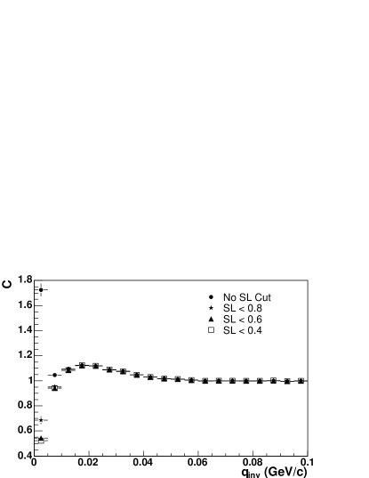
Figure 2: 1D correlation function for different values of SL (anti-splitting cut). The cut applied in the analysis is SL $<$ 0.6. The horizontal lines indicate the bin width.

We required every pair to have SL smaller than a certain value. This value was determined from the 1-dimensional correlation functions as a function of the relative momentum of the pair $q_{\textrm{inv}}$, for different values of SL; some of them are shown in Fig. 2. The relative momentum of the pair is defined as $q_{\textrm{inv}}=\sqrt{(q^{0})^{2}-|\vec{q}|^{2}}$ where $q^{0}$ and $\vec{q}$ are the components of the four-vector momentum difference. We observe that when making this cut more restrictive (reducing the maximum allowed value for SL) the enhancement is reduced until we reach SL = 0.6 when the correlation function becomes stable and does not change for lower values of SL. Therefore, all the pairs entering the correlation functions were required to have SL $<$ 0.6. Cutting at this value is also supported by simulation studies. While naturally track splitting can only give rise to false pairs, our SL cut also removes some real pairs which happen to satisfy the cut. Therefore, we apply the SL cut to both, “real” and “mixed” pairs, numerator and denominator of $C(\vec{q})$, Eq. (1).

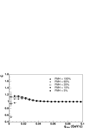
Figure 3: 1D correlation function for different values of the maximum fraction of merged hits allowed. Cut applied in the analysis is fraction of merged hits (FMH) $<$ 10%. The horizontal lines indicate the bin width.

II.4.2 Merged tracks

Once we have removed split tracks we can study the effects of two particles reconstructed as one track. These merged tracks cause a reduction of pairs at low relative momentum since the particles that have higher probability of being merged are those with similar momenta. To eliminate the effect of track merging, we required that all pairs entering numerator and denominator of the correlation function had a fraction of merged hits no larger than 10%. Two hits are considered merged if the probability of separating them is less than 99%. From simulation and data studies, this minimum separation was determined to be 5 mm. By applying this cut to “real” and “mixed” pairs, we introduce in the denominator the effect that merged tracks have in the numerator: a reduction of low q pairs. Note that tracks from different events will originate from primary vertices at different positions along the beam direction. Thus, even two tracks with identical momenta, which would surely be merged if they originated from the same event, may not be considered as a merged track when they formed a “mixed” pair if we would not account for the different primary vertex position. Our procedure is to calculate (using a helix model) the pad-row hit positions of each track, assuming that the track originated at the center of the TPC LOPEZ04 . These calculated hit positions are used in the merging cut procedure described above. By applying this cut to the numerator, we would remove “real” pairs that satisfy the cut. This would reduce the HBT fit parameters for a correlation function that is not completely Gaussian, and needs to be taken into account as will be described in the next section.

To determine the maximum fraction of merged hits allowed we proceed as we did for the anti-splitting cut. Figure 3 shows the 1-dimensional correlation functions as a function of $q_{\textrm{inv}}$, for different values of the maximum fraction of merged hits allowed. By requiring the fraction of merged hits to be less than 10% for every pair entering the correlation function, the effect of merged tracks in the correlation function was almost completely removed as will be discussed in section III.

II.4.3 $k_{T}$ cut and pair binning

As already mentioned, no explicit $p_{T}$ cut was applied to single tracks beyond the requirement for clean PID. However, in addition to the two cuts already described, pairs were required to have an average transverse momentum ($k_{T}=(|\vec{p}_{1T}|+|\vec{p}_{2T}|)/2$) between 150 and 600 MeV/c. No difference was observed between the extracted HBT parameters when applying equivalent $p_{T}$ or $k_{T}$ cuts. However statistics improved when using the latter cut, as two pions from different $p_{T}$ bins will be used in a $k_{T}$-cut analysis, but not in a $p_{T}$-cut analysis.

Pairs were then binned by $k_{T}$ in 4 bins that correspond to [150,250] MeV/c, [250,350] MeV/c, [350,450] MeV/c, and [450,600] MeV/c. Here the results are presented as a function of the average $k_{T}$ (or $m_{T}=\sqrt{k_{T}^{2}+m_{\pi}^{2}}$) in each of those bins.

In addition, in the azimuthally-sensitive HBT analysis, to observe the particle source from a series of angles, pairs were also binned according to the angle $\Phi=\phi_{\textrm{pair}}-\Psi_{2}$, where $\phi_{\textrm{pair}}$ is the azimuthal angle of the pair transverse momentum $\vec{k}_{T}$ and $\Psi_{2}$ is the second-order event plane azimuthal angle. The first-order event plane angle is not reconstructible with the STAR detector configuration for this analysis. Because we use the second-order reaction plane, $\Phi$ is only defined in the range [0,$\pi$].

III Analysis method

III.1 Construction of correlation function

The two-particle correlation function between identical bosons with momenta $\vec{p}_{1}$ and $\vec{p}_{2}$ is defined in Eq. (1). As already mentioned, $A(\vec{q})$ is the measured distribution of the momentum difference for pairs of particles from the same event and $B(\vec{q})$ is obtained by mixing particles in separate events KOPYL77 and represents the product of single particle probabilities. Each particle in one event is mixed with all the particles in a collection of events which in our case consists of 20 events. As discussed before, events in a given collection have primary vertex $z$ position within 5 cm, multiplicities within 5 to 30% of each other, and, for the azimuthally-sensitive analysis, estimated reaction plane orientations within $20^{\circ}$.

III.2 Pratt-Bertsch parametrization

In order to probe length scales differentially in beam and transverse directions, the relative momentum $\vec{q}$ is usually decomposed in the Pratt-Bertsch (or “out-side-long”) convention BERTS98 ; PRATT86 ; CHAPMA95 . In this parametrization the relative momentum vector of the pair $\vec{q}$ is decomposed into a longitudinal direction along the beam axis, $q_{l}$, an outward direction parallel to the pair transverse momentum, $q_{o}$, and a sideward direction perpendicular to those two, $q_{s}$.

We choose as the reference frame, the longitudinal comoving system (LCMS) frame of the pair, in which the longitudinal component of the pair velocity vanishes. At midrapidity, in the LCMS frame, and with knowledge of the second-order but not the first-order reaction plane, the correlation function is usually parameterized by a 3-dimensional Gaussian in the relative momentum components as HEINZ02b :

$$C(\vec{q})=1+\lambda e^{-q_{o}^{2}R_{o}^{2}-q_{s}^{2}R_{s}^{2}-q_{l}^{2}R_{l}^{2}-2q_{o}q_{s}R_{os}^{2}}.$$ (4)

For an azimuthally integrated analysis, the correlation function is symmetric under $q_{s}\rightarrow-q_{s}$ and $R_{os}^{2}=0$.

In principle, the possibility that the emission of particles is neither perfectly chaotic nor completely coherent can be taken into account by adding the parameter $\lambda$ to the correlation function, which, in general, depends on $k_{T}$. This $\lambda$ parameter should be unity for a fully chaotic source and smaller than unity for a source with partially coherent particle emission. In the analysis presented here we have assumed completely chaotic emission ADAMS03e and attribute the deviations from $C(q=0,k)=2$ to contribution from pions coming from long-lived resonances, and misidentified particles, such as electrons.

While for the azimuthally integrated analysis the sign of the $\vec{q}$ components is arbitrary, in the azimuthally-sensitive analysis, the sign of $R_{os}^{2}$ is important because it tells us the azimuthal direction of the emitted particles, so the signs of $q_{o}$ and $q_{s}$ are kept and particles in every pair are ordered such that $q_{l}>0$.

References WIEDE98 ; WIEDE99 give a detailed description of the relation between the HBT radius parameters ($R_{o}^{2}$, $R_{s}^{2}$, $R_{l}^{2}$ and $R_{os}^{2}$) and the space-time geometry of the final freeze-out stage.

III.3 Fourier components

For a boost-invariant system, the $\Phi$ dependence of the HBT radii of Eq. (4) are HEINZ02b :

$$R_{\mu}^{2}(k_{T},\Phi)=R_{\mu,0}^{2}(k_{T})+{}$$

$${}2\sum_{n=2,4,6\cdots}R_{\mu,n}^{2}(k_{T})\cos(n\Phi)~{}~{}~{}(\mu=o,s,l){}$$

$$R_{\mu}^{2}(k_{T},\Phi)={}$$ (5)

$${}2\sum_{n=2,4,6\cdots}R_{\mu,n}^{2}(k_{T})\sin(n\Phi)~{}~{}~{}(\mu=os),$$

where $R_{\mu,n}(k_{T})$ are the $n^{\textrm{th}}$ order Fourier coefficients for the $\mu$ radius. These coefficients, that are $\Phi$ independent, can be calculated as:

$$R_{\mu,n}^{2}(k_{T})=\Bigg{\{}\begin{array}[]{ll}\langle R_{\mu}^{2}(k_{T},\Phi)\cos(n\Phi)\rangle&(\mu=o,s,l)\\ \langle R_{\mu}^{2}(k_{T},\Phi)\sin(n\Phi)\rangle&(\mu=os).\end{array}$$ (6)

As we will show, the $0^{\textrm{th}}$ order Fourier coefficients correspond to the extracted HBT radii in an azimuthally integrated analysis. In this analysis we found that Fourier coefficients above $2^{\textrm{nd}}$ order are consistent with 0.

III.4 Coulomb interaction and fitting procedures

Equation (4) applies only if the sole cause of correlation is quantum statistics and the correlation function is Gaussian. We come to this second point in section IV.1. In our case, significant Coulomb effects must also be accounted for (strong interactions are within reasonable limit here WIEDE99 ). This Coulomb interaction between pairs, repulsive for like-sign particles, causes a reduction in the number of real pairs at low $q$ reducing the experimental correlation function as seen in Fig. 4.

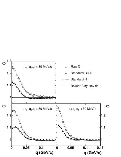
Figure 4: Projections of the 3 dimensional correlation function and corresponding fits for negative pions from the 0–5% most central events and $k_{T}$ = [150,250] MeV/c according to the standard and Bowler-Sinyukov procedures.

III.4.1 Standard procedure

Three different procedures can be applied in order to take this interaction into account. One procedure that was used in our analysis at $\sqrt{s{NN}}$ = 130 GeV ADLER01 as well as by previous experiments, consists of fitting the correlation function to

$$C(q_{o},q_{s},q_{l})=\frac{A(\vec{q})}{B(\vec{q})}=K_{\textrm{coul}}(q_{\textrm{inv}})\times$$

$$(1+\lambda e^{-q_{o}^{2}R_{o}^{2}-q_{s}^{2}R_{s}^{2}-q_{l}^{2}R_{l}^{2}-2q_{o}q_{s}R_{os}^{2}}),$$

normalized to unity at large $\vec{q}$, where $K_{\textrm{coul}}$ is the squared Coulomb wave-function integrated over the whole source, which in our case is a spherical Gaussian source of 5 fm radius. The effect on the final results of changing the radius of the spherical Gaussian source to calculate $K_{\textrm{coul}}$ was studied and found to be within reasonable limits. Traditionally, Eq. (III.4.1) has been expressed as

$$C^{\prime}(q_{o},q_{s},q_{l})=\frac{A(\vec{q})}{B(\vec{q})K_{\textrm{coul}}(q_{\textrm{inv}})}$$

$$=1+\lambda e^{-q_{o}^{2}R_{o}^{2}-q_{s}^{2}R_{s}^{2}-q_{l}^{2}R_{l}^{2}-2q_{o}q_{s}R_{os}^{2}},$$

and this new correlation function was called the Coulomb corrected correlation function since we introduce in the denominator a Coulomb factor with which we try to compensate the Coulomb interaction in the numerator. We call this standard procedure. However, this procedure overcorrects the correlation function since it assumes that all pairs in the background are primary pairs and need to be corrected PRATT86b .

III.4.2 Dilution procedure

In a second procedure, inspired by the previous procedure and implemented before by the E802 collaboration AHLE02 , the Coulomb term is “diluted” according to the fraction of pairs that Coulomb interact as:

$$K_{\textrm{coul}}^{\prime}(q_{\textrm{inv}})=1+f(K_{\textrm{coul}}(q_{\textrm{inv}})-1),$$ (9)

where $f$ has a value between 0 (no Coulomb weighting) and 1 (standard weight). The correlation function in this procedure is fitted to:

$$C(q_{o},q_{s},q_{l})=\frac{A(\vec{q})}{B(\vec{q})}=K_{\textrm{coul}}^{\prime}(q_{\textrm{inv}})\times$$

$$(1+\lambda e^{-q_{o}^{2}R_{o}^{2}-q_{s}^{2}R_{s}^{2}-q_{l}^{2}R_{l}^{2}-2q_{o}q_{s}R_{os}^{2}}),$$

normalized to unity at large $\vec{q}$. We call this the dilution procedure. A reasonable assumption is to take $f=\lambda$ assuming that $\lambda$ is the fraction of primary pions. This increases $R_{o}$ by 10–15% and has a very small effect on $R_{s}$ and $R_{l}$ as seen in Fig. 5. $\lambda$ decreases by 10–15%.

III.4.3 Bowler-Sinyukov procedure

An advantage of the previous two techniques is that after “correcting” for Coulomb effects, one winds up with a correlation function which may be fit with a simple Gaussian form. However if there exists more than one source of interaction, it is not valid to “correct” one way. For example, it is, in fact, the same pion pairs which Coulomb interact as which show quantum enhancement. This leads to a change in the expected form of the correlation function if not all particles participate in the interaction (i.e., $\lambda\neq 0$) NOTE2 . If $\lambda=1$, all three methods are equivalent.

In this analysis, we have implemented a new procedure, first suggested by Bowler BOWL91 and Sinyukov et al. SINY98 , and recently advocated by the CERES collaboration ADAMO03 , in which only pairs with Bose-Einstein interaction are considered to Coulomb interact. The correlation function in this procedure is fitted to:

$$C(q_{o},q_{s},q_{l})=\frac{A(\vec{q})}{B(\vec{q})}=(1-\lambda)+$$

$$\lambda K_{\textrm{coul}}(q_{\textrm{inv}})(1+e^{-q_{o}^{2}R_{o}^{2}-q_{s}^{2}R_{s}^{2}-q_{l}^{2}R_{l}^{2}-2q_{o}q_{s}R_{os}^{2}}),$$

normalized to unity at large $\vec{q}$, where $K_{\textrm{coul}}(q_{\textrm{inv}})$ is the same as in the standard procedure. The first term on the right-hand side of Eq. (III.4.3) accounts for the pairs that do not interact and the second term for the pairs that (Coulomb and Bose-Einstein) interact. We call this Bowler-Sinyukov procedure. It has a similar effect on the HBT parameters as the dilution procedure as seen in Fig. 5. A similar procedure has been recently implemented by the Phobos collaboration BACK04 . In this procedure only pairs which are close in the pair center of mass frame are considered to Coulomb interact.

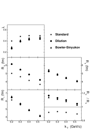
Figure 5: HBT parameters for the three possible fitting procedures to the correlation functions described in this paper depending on how Coulomb interaction is taken into account from the 0–5% most central events. Error bars contain only statistical uncertainties.

It is worth mentioning that the parameters $\lambda$ and $R_{o}$, and consequently the ratio $R_{o}/R_{s}$, extracted using the standard procedure here are smaller than the parameters obtained in our previous analysis ADLER01 . This is explained by a different particle selection. In the analysis presented here, the contribution from non-primary pions is larger than in the previous analysis, leading to smaller $\lambda$ and $R_{o}$ when using that procedure. However, the parameters obtained when applying the Bowler-Sinyukov procedure are almost not affected by the contribution from non-primary pions.

III.4.4 Comparison of methods

Figure 4 shows the projections of the 3-dimensional correlation function according to the Pratt-Bertsch parametrization described in section III.2 for an azimuthally integrated analysis. The closed symbols represent the correlation function and the open symbols the Coulomb corrected correlation function according to the standard procedure. The lines are fits to the data, the dashed line is the standard fit to the Coulomb corrected correlation function, and the continuous line the Bowler-Sinyukov fit to the uncorrected correlation function. The extracted parameters from both fits are the parameters for the lowest $\langle k_{T}\rangle$ in Fig. 5.

As a consistency check for the Bowler-Sinyukov procedure, we calculated the $\pi^{+}\pi^{-}$ correlation function, dominated by Coulomb interaction, and compare to different calculations. In Fig. 6 lines indicate the standard ($K_{c\textrm{oul}}(q_{\textrm{inv}})$) and Bowler-Sinyukov ($(1-\lambda)+\lambda K_{\textrm{coul}}(q_{\textrm{inv}})$) Coulomb functions where $\lambda$ was extracted from the fit to the 3D like-sign correlation function. This latter $\lambda$ is the same $\lambda$ as dilution for unlike sign pions and takes into account the percentage of primary pions through $\lambda$. Clearly, the Bowler-Sinyukov function (thick line) better reproduces the data (closed symbols) than the standard function (thin line). The small discrepancy between the Bowler-Sinyukov function and the data disappears when strong interaction (negligible for like-sign pions) is added to the Bowler-Sinyukov function as shown by the theoretical calculation LEDNI82 (open symbols). Between identical pions, there is a repulsive s-wave interaction for the isospin I=2 system BOWLE88 . However, the range of this interaction is estimated to be $\sim$ 0.2 fm, while the characteristic separation between pions in heavy ions collisions is $\sim$ 5 fm. Also, there are no doubly charged mesonic resonances that could decay into same charged pions that would strongly interact. For these reasons, the strong interaction will be ignored for like sign particles.

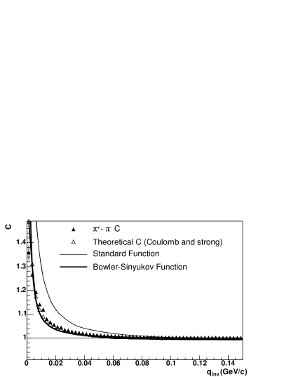
Figure 6: 1D correlation function for $\pi^{+}\pi^{-}$ compared to Standard, Bowler-Sinyukov functions and a theoretical calculation that includes Coulomb and strong interactions.

III.4.5 Coulomb interaction with the source

The Coulomb interaction between the outgoing charged pions and the residual positive charge in the source is negligible WZAJC84 ; HBARZ99 . This is confirmed by the good agreement observed between the parameters extracted from $\pi^{+}\pi^{+}$ and $\pi^{-}\pi^{-}$ correlation functions as shown later in this paper, Fig. 14.

III.5 Momentum resolution correction

The limited single-particle momentum resolution induces broadening of the correlation function and thus systematic underestimation of the HBT parameters. To determine the magnitude of this effect we need to know the momentum resolution for the particles under consideration. We estimate our single-particle momentum resolution by embedding simulated particles into real events at the TPC pixel level and comparing the extracted and input momenta. Figure 7 shows the RMS spreads as a function of $|\vec{p}|$ in $p_{T}$ and angles $\phi$ and $\theta$, where $\theta$ is the angle between the momentum of the particle and the beam axis and $\phi$ is the azimuthal angle of the particle. We see that the resolution in $p_{T}$, given by $\delta p_{T}/p_{T}$ (top panel of Fig. 7), has a width of about 1% for the momentum range under consideration.

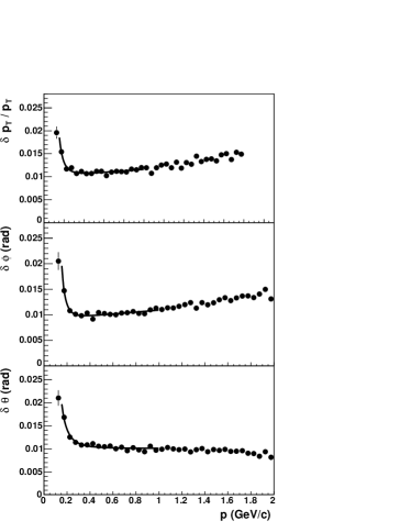
Figure 7: Momentum resolution for pions at midrapidity expressed by the widths $\delta p_{T}/p_{T}$, $\delta\varphi$ and $\delta\theta$ as a function of $p$.

To account for this limited momentum resolution, a correction, $K_{\textrm{momentum}}(\vec{q})$, is applied to each measured correlation function:

$$C(\vec{q}_{\textrm{}})=\frac{A(\vec{p}_{1\textrm{meas}},\vec{p}_{2\textrm{meas}})}{B(\vec{p}_{1\textrm{meas}},\vec{p}_{2\textrm{meas}})}K_{\textrm{momentum}}(\vec{q}).$$ (12)

The correction factor is calculated from the single-particle momentum resolution as follows:

$$K_{\textrm{momentum}}(\vec{q})=\frac{C(\vec{q}_{\textrm{ideal}})}{C(\vec{q}_{\textrm{smear}})}\\ =\frac{\frac{A(\vec{p}_{1\textrm{ideal}},\vec{p}_{2\textrm{ideal}})}{B(\vec{p}_{1\textrm{ideal}},\vec{p}_{2\textrm{ideal}})}}{\frac{A(\vec{p}_{1\textrm{smear}},\vec{p}_{2\textrm{smear}})}{B(\vec{p}_{1\textrm{smear}},\vec{p}_{2\textrm{smear}})}},$$

where the ideal and smear correlation function are formed as follows. Numerator and denominator of the ideal correlation function are formed by pairs of pions from different events. Each pair in the numerator is weighted, according with the Bowler-Sinyukov function, by:

$$weight=(1-\lambda)+\lambda K_{\textrm{coul}}(q_{\textrm{inv}})\times{}$$ (13)

$$(1+e^{-q_{o}^{2}R_{o}^{2}-q_{s}^{2}R_{s}^{2}-q_{l}^{2}R_{l}^{2}-2q_{o}q_{s}R_{os}^{2}}),$$

where $K_{\textrm{coul}}(q_{\textrm{inv}})$ is the same factor as described in section III.4 and $R_{os}^{2}$ = 0 in the azimuthally integrated analysis. If the measured momentum were the “real” momentum, this ideal correlation function would be the “real” correlation function. However this is not the case, so we calculate a smeared correlation function for which numerator and denominator are also formed by pairs of pions from different events but their momenta have been smeared according to the extracted momentum resolution. Pairs in the numerator are also weighted by the $weight$ given by (13). This smeared correlation function is to the ideal correlation function, as our “measured” correlation function is to the “real” correlation function, which allows us to calculate the correction factor.

For the $weight$, certain values for the HBT parameters ($\lambda$, $R_{o}$, $R_{s}$, $R_{l}$ and $R_{os}$) need to be assumed. Therefore, this procedure is iterative with the following steps:

1. Fit the correlation function without momentum resolution correction, and use the extracted HBT parameters for the first $weight$.

2. Construct the momentum resolution corrected correlation function.

3. Fit it according to Eq. (III.4.3).

4. If the extracted parameters agree with the parameters used to calculate the $weight$, those are the final parameters. If they differ from the parameters used, then use these latter extracted parameters for the new weight and go back to step 2.

Also, to be fully consistent, the Coulomb factor $K_{\textrm{coul}}(q_{\textrm{inv}})$ (where $q_{\textrm{inv}}$ is calculated from pairs of pions from different events) used in the fit to extract the HBT parameters must be modified to account for momentum resolution as follows:

$$K_{\textrm{coul}}(q_{\textrm{inv}}){}$$ (14)

$$=K_{\textrm{coul}}(q_{\textrm{inv,meas}})\frac{K_{\textrm{coul}}(q_{\textrm{inv,ideal}})}{K_{\textrm{coul}}(q_{\textrm{inv,smear}})}$$

$$=\frac{K_{\textrm{coul}}^{2}(q_{\textrm{inv,meas}})}{K_{\textrm{coul}}(q_{\textrm{inv,smear}})}.$$

For this analysis, after two iterations the extracted parameters were consistent with the input parameters. We also checked that when convergence is reached, the “uncorrected” HBT parameters matched the smeared parameters. The correction increases the HBT radius parameters between 1.0% for the lowest $k_{T}$ bin [150,250] MeV/c and 2.5% for the highest bin [450,600] MeV/c.

III.6 $\Phi$-dependent HBT analysis methods

The study of HBT radii relative to the reaction plane angle was performed ADAMS03c by extending the analysis techniques as presented in this section, to account for reaction plane resolution and small instabilities in the fits. We discuss these here. For the azimuthally-sensitive analysis, each of the four radii extracted from the Bowler-Sinyukov fit contains an implicit dependence on the azimuthal angle $\Phi$ between the pion pair and the reaction plane. Azimuthally-sensitive studies of the HBT radii $\bigl{(}R_{\mu}(\Phi)\bigr{)}$ ADAMS03c also must correct for finite resolution when estimating the true reaction plane $\Psi_{\rm rp}$ HEINZ02b . Finite reaction plane resolution acts to decrease the measured amplitude of the radii oscillations, similar to its effect on azimuthal particle distributions relative to the reconstructed event plane $\Psi_{2}$ (i.e., elliptic flow ACKER01 ). The technique for the resolution correction, which also corrects for finite $\Phi$-bin width, was developed extensively in Ref. HEINZ02b . Here we discuss briefly how this correction is implemented and the resulting effect on the HBT radii.

The basic principle behind the correction procedure is that, for a given ${\vec{q}}$-bin in the numerator $A(\vec{q})$ and denominator $B(\vec{q})$ of each correlation function, the measured contents for that ${\vec{q}}$-bin at different $\Phi$ are modified due to the $\Psi_{\rm rp}$ resolution. The true angular dependence of $\Phi$ (for each ${\vec{q}}$-bin) can be extracted from the measured $\Phi_{j}$ by performing a Fourier decomposition of $A(\vec{q})$ and $B(\vec{q})$, which leads to the correction factors HEINZ02b

$$A_{\alpha,n}^{\Delta}(\vec{q}) = A_{\alpha,n}(\vec{q})\frac{\sin(n\Delta/2)}{n\Delta/2},$$ (15)

$$A^{\textrm{exp}}_{\alpha,n}(\vec{q}) = A_{\alpha,n}^{\Delta}(\vec{q})\bigl{\langle}\cos\left(n(\Psi_{2}{-}\Psi_{\textrm{rp}})\right)\bigr{\rangle},$$

where $\alpha$ refers to both cosine and sine series, $\Delta$ is the width of each $\Phi$ bin, and $n$ is the Fourier component. The factors $\langle\cos\left(n(\Psi_{2}{-}\Psi_{\rm rp})\right)\rangle$ are the well-known correction factors for event plane resolution, obtained by extracting the anisotropic flow coefficients $v_{n}$ from the single particle spectrum VOLOS96c ; POSKA98 . The same procedure is used to correct the denominator $B(\vec{q})$.

In the present analysis, only the 2nd-order event plane ($\Psi_{2}$) is measured. Using Eq. (15), the numerator $A(\vec{q})$ and denominator $B(\vec{q})$ for each ${\vec{q}}$-bin at each measured angle $\Phi_{j}$ can be corrected for both the effects of angular binning and finite event plane resolution:

$$A(\vec{q},\Phi_{j})~{}=~{}N_{\textbf{exp}}(\vec{q},\Phi_{j})~{}+~{}~{}~{}~{}~{}~{}$$

$$2~{}\sum_{n=1}^{n_{\textrm{bin}}}\zeta_{2}(\Delta)\Big{[}A^{\textrm{exp}}_{c,2}(\vec{q})\cos(2\Phi_{j})~{}+$$ (16)

$$A^{\textrm{exp}}_{s,2}(\vec{q})\sin(2\Phi_{j})\Big{]},~{}~{}~{}~{}~{}~{}~{}~{}~{}~{}~{}~{}~{}~{}~{}~{}~{}~{}~{}~{}~{}~{}$$

with the correction parameter $\zeta_{2}(\Delta)$ given by

$$\zeta_{2}(\Delta)=\frac{\Delta}{\sin(\Delta)\langle\cos(2(\Psi_{2}{-}\Psi_{\rm rp}))\rangle_{p}}-1.$$ (17)

The procedure is model independent; the quantities on the right hand side of Eq. (III.6) are all measured experimentally.

For each set of $\Phi_{j}$ histograms, the correction procedure modifies both the numerators and denominators, and therefore the correlation functions as well.

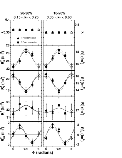
Figure 8: Squared HBT radii relative to the reaction plane angle, without and with the reaction plane resolution applied, for two different centrality-$k_{T}$ ranges. The solid lines show allowed fits to the individual oscillations.

Figure 8 shows the squared HBT radii, obtained using Eq. (III.3), as a function of $\Phi$ for two combinations of centrality and $k_{T}$. In each case, the oscillation amplitudes for the three transverse radii increases after the resolution correction has been applied, while the mean shows little change.

An additional technique employed in the azimuthally-sensitive HBT analysis is to use a common $\lambda$ parameter for each centrality/$k_{T}$ bin. This step was undertaken to improve the quality of the fits by restricting the $\lambda$ parameter, under the assumption that $\lambda$ should have no implicit $\Phi$ dependence. For an analysis with four $\Phi$ bins, this effectively reduces the number of free parameters per centrality/$k_{T}$ bin (after normalization) from 20 [(4 radii + $\lambda$) $\times N_{\Phi}$] to 17 [(4 radii $\times N_{\Phi}$) + $\lambda$]. Since fitting all four correlation functions with a 17-parameter function is arduous, we determined the average $\lambda$ parameter from the four fits and then re-fit each of the four correlation functions with $\lambda$ fixed to its average.

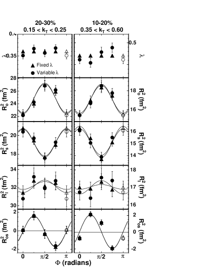
Figure 9: Squared HBT radii relative to the reaction plane angle, for the case where the $\lambda$ parameter is averaged and fixed in the fit, and the case where $\lambda$ is a free fit parameter for each $\Phi$. The solid lines show allowed fits to the individual oscillations.

Figure 9 compares the fit parameters obtained with and without averaging/fixing $\lambda$, for two centrality/$k_{T}$ ranges. While the individual radii show some deviations, the resulting Fourier coefficients (which are represented by the symmetry-constrained drawn in Fig. 9) are consistent within errors for the two methods.

III.7 Systematic uncertainties associated with pair cuts

The maximum fraction of merged hits cut described in section II.4 introduces a systematic variation on the HBT fit parameters $\lambda$, $R_{o}^{2}$, $R_{s}^{2}$, and $R_{l}^{2}$, since it discriminates against low-$q$ pairs which carry the correlation signal. This is a consequence of the non-Gaussianess of the correlation function. If it were a perfect Gaussian, this cut would not change the extracted parameters from the Gaussian fit, it would only reduce the statistics in certain bins and therefore the only effect would be an increase in the statistical errors.

Figure 10: For $\pi^{-}\pi^{-}$ ($\pi^{+}\pi^{+}$), merging occurs more often between tracks with $|q_{o}q_{s}|=q_{o}q_{s}$ ($|q_{o}q_{s}|\neq q_{o}q_{s}$) than with $|q_{o}q_{s}|\neq q_{o}q_{s}$ ($|q_{o}q_{s}|=q_{o}q_{s}$). Note that exchanging the designations “1” and “2” does not change the sign of $q_{o}q_{s}$.

In order to estimate this reduction we define a range in the number of merged hits in which the lower limit is 0 (i.e., no merging) and the higher limit is the value for which we consider there is too much merging. This value is determined from the $0^{\textrm{th}}$ order Fourier coefficients, $R_{os,0}^{2}$ which is expected to be 0, Eq. (6). However, track merging introduces a deviation of $R_{os}^{2}$ away from 0 caused by the preferential merging of track pairs with correlated transverse momenta, $q_{o}$ and $q_{s}$ as shown in Fig. 10. If we calculate the components of $\vec{q}$ in the plane transverse to the beam as $\vec{p}_{T,1}-\vec{p}_{T,2}$ where index 1 denotes the stiffer track and define $\vec{\hat{\rho}}$ as the direction of the radius of curvature of the stiffer track, then if $\vec{q}\cdot\vec{\hat{\rho}}$ is positive there is more merging on average. In the case of $\pi^{-}\pi^{-}$ pairs, there is a higher degree of track merging when $|q_{o}q_{s}|$ = $q_{o}q_{s}$ than when $|q_{o}q_{s}|$ $\neq$ $q_{o}q_{s}$ (top pairs). For $\pi^{+}\pi^{+}$ pairs the conditions are opposite (bottom pairs).

When $R_{os}^{2}$ for $\pi^{+}$ or $\pi^{-}$ analysis clearly deviates from 0, we consider that there is too much merging and use that value of the maximum fraction of merged hits as the upper limit of the range. We calculate the change of each HBT radius in this range and consider that to be the artificial reduction due to the cut for that specific parameter. This reduction is included as a systematic error in the final value. This is done for each centrality and each $k_{T}$ bin.

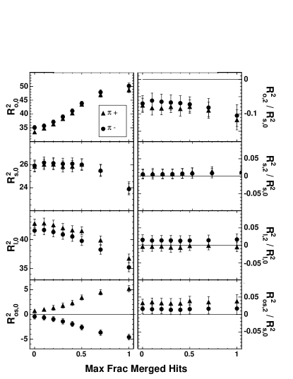
Figure 11: Fourier coefficients as a function of the maximum fraction of merged hits for the 5% most central events and $k_{T}$ between 150 and 250 MeV/c.

As an example, Fig. 11 shows the $0^{\textrm{th}}$ order (left) and $2^{\textrm{nd}}$ divided by $0^{\textrm{th}}$ order (right) Fourier coefficients as a function of the maximum fraction of merged hits allowed for the 5% most central events and 150 $<~{}k_{T}~{}<$ 250 MeV. From $R_{os,0}^{2}$, located in the bottom left panel, we determined the upper limit of merged fraction to be 0.2 and the corresponding variations in the HBT radii to be 7% for $R_{o}$, 5% for $R_{s}$ and 10% for $R_{l}$. The systematic errors calculated according to this method are less or equal than 10% for all radii, in all centralities and $k_{T}$ bins.

IV Pion HBT at $\sqrt{s{NN}}$ = 200 GeV

IV.1 How Gaussian is the measured correlation function?

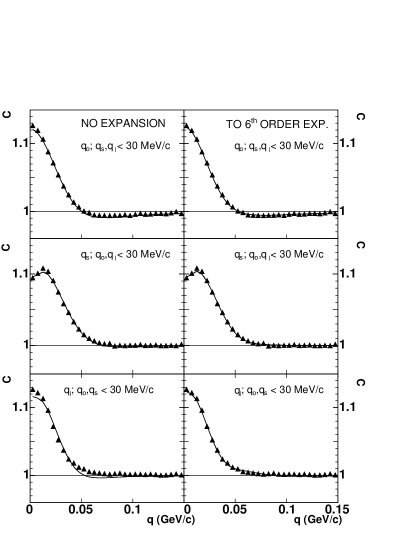
Figure 12: Projections of the 3 dimensional correlation functions and fits to Eq. (III.4.3) (left) and with the Edgeworth expansion to Eq. (18) to $6^{\textrm{th}}$ order (right).

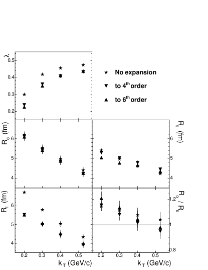
Figure 13: HBT parameters for 0–5% most central events for fits to Eq. (III.4.3) and to Eq. (18) to $4^{\textrm{th}}$ and to $6^{\textrm{th}}$ orders. Error bars reflect only statistical uncertainties.

Interferometric length scales are usually extracted from measured correlation functions by fitting to a Gaussian functional form, as discussed in III. However, there is no reason to expect the measured correlation function to be completely Gaussian, and it is well-known that it seldom is. Seemingly-natural questions such as “how non-Gaussian is the correlation function?” “how does the non-Gaussianness affect extracted length scales?” or “what is the shape of the correlation function?” have, unfortunately, no unique, assumption-free answers.

Often, non-Gaussian features are simply ignored in experimental analyses. Alternatively, the effect of non-Gaussianness is estimated (e.g. by varying the range of $q$-values used in the fit) and quoted as a systematic error on the HBT radii. Occasionally, some alternative functional form (e.g. a sum of two Gaussians, or an exponential plus a Gaussian) is chosen ad-hoc by the experimenter based on the general “appearance” of the data.

One disadvantage of this last approach is the difficulty in systematically comparing HBT results obtained with different functional forms. Since one might hope for evidence of “new” physics at RHIC, it is important to place RHIC HBT results into the context of previously-established systematics. Thus this paper mainly focusses on Gaussian HBT radius systematics. However, to address non-Gaussian issues, here we move beyond ad-hoc methods and adopt as a standard the Edgeworth expansion proposed by Csörgő and collaborators CSORG99 ; CSORG00 ; CSORG03 . Using the Bowler-Sinyukov Coulomb treatment, the correlation functions are fitted to

$$C(q_{o},q_{s},q_{l})=(1-\lambda)+\lambda K_{\textrm{coul}}(q_{\textrm{inv}})$$ (18)

$$+\lambda K_{\textrm{coul}}(q_{\textrm{inv}})\cdot e^{-q_{o}^{2}R_{o}^{2}-q_{s}^{2}R_{s}^{2}-q_{l}^{2}R_{l}^{2}}\times$$

$$\Big{[}1+\sum_{n=4,\textrm{n~{}even}}^{\infty}\frac{\kappa_{o,n}}{n!(\sqrt{2})^{n}}H_{n}(q_{o}R_{o})\Big{]}\times$$

$$\Big{[}1+\sum_{n=4,\textrm{n~{}even}}^{\infty}\frac{\kappa_{s,n}}{n!(\sqrt{2})^{n}}H_{n}(q_{s}R_{s})\Big{]}\times$$

$$\Big{[}1+\sum_{n=4,\textrm{n~{}even}}^{\infty}\frac{\kappa_{l,n}}{n!(\sqrt{2})^{n}}H_{n}(q_{l}R_{l})\Big{]},$$

where $\kappa_{i,n}$ ($i=o,s,l$) are fit parameters and $H_{n}(q_{i}R_{i})$ are the Hermite polynomials of order n:

$$H_{n}(x)=(-1)^{n}e^{x^{2}}\frac{d^{n}}{dx^{n}}~{}e^{-x^{2}}.$$ (19)

Only Hermite polynomials of even order are included in the expansion because the correlation function for identical particles must be invariant under $(q_{o},q_{s},q_{l})~{}\rightarrow~{}(-q_{o},-q_{s},-q_{l})$.

At midrapidity and integrated over azimuthal angle, the quantum interference term is factorizable into the $q_{o}$, $q_{s}$, and $q_{l}$ variables. Therefore, it may be uniquely decomposed in terms of any complete set of basis functions of these variables. Given a sufficient number of terms, any basis set will do. Thus, the potential advantage of the Edgeworth decomposition (Eq. 18) is not that it is any more “model-independent” CSORG00 than, say, a Tschebyscheff decomposition, but that a functional expansion about a Gaussian shape might most economically describe the data. Since they are approximately Gaussian, one hopes to capture the shape of measured correlation functions with only a few low-order terms.

$k_{T}$ (MeV/c)	150–250	250–350	350–450	450–600
$\lambda$	0.30 $\pm$ 0.01	0.42 $\pm$ 0.01	0.45 $\pm$ 0.01	0.47 $\pm$ 0.01
$\lambda$ ($4^{\textrm{th}}$ ord.)	0.24 $\pm$ 0.01	0.36 $\pm$ 0.01	0.41 $\pm$ 0.01	0.43 $\pm$ 0.01
$\lambda$ ($6^{\textrm{th}}$ ord.)	0.23 $\pm$ 0.01	0.35 $\pm$ 0.01	0.41 $\pm$ 0.01	0.44 $\pm$ 0.01
$R_{o}$	6.16 $\pm$ 0.01	5.51 $\pm$ 0.01	4.88 $\pm$ 0.02	4.32 $\pm$ 0.02
$R_{o}$ ($4^{\textrm{th}}$ ord.)	6.07 $\pm$ 0.04	5.40 $\pm$ 0.03	4.75 $\pm$ 0.03	4.14 $\pm$ 0.04
$\kappa_{o,4}$	0.37 $\pm$ 0.05	0.36 $\pm$ 0.04	0.33 $\pm$ 0.05	0.40 $\pm$ 0.06
$R_{o}$ ($6^{\textrm{th}}$ ord.)	6.05 $\pm$ 0.05	5.40 $\pm$ 0.04	4.78 $\pm$ 0.04	4.17 $\pm$ 0.04
$\kappa_{o,4}$	0.53 $\pm$ 0.11	0.45 $\pm$ 0.10	0.20 $\pm$ 0.11	0.22 $\pm$ 0.13
$\kappa_{o,6}$	0.83 $\pm$ 0.39	0.53 $\pm$ 0.38	0.63 $\pm$ 0.44	–0.84 $\pm$ 0.53
$R_{s}$	5.39 $\pm$ 0.01	4.93 $\pm$ 0.01	4.53 $\pm$ 0.01	4.14 $\pm$ 0.02
$R_{s}$ ($4^{\textrm{th}}$ ord.)	5.27 $\pm$ 0.03	4.98 $\pm$ 0.03	4.68 $\pm$ 0.03	4.36 $\pm$ 0.03
$\kappa_{s,4}$	0.22 $\pm$ 0.04	–0.03 $\pm$ 0.04	–0.27 $\pm$ 0.04	–0.50 $\pm$ 0.05
$R_{s}$ ($6^{\textrm{th}}$ ord.)	5.01 $\pm$ 0.05	4.74 $\pm$ 0.04	4.57 $\pm$ 0.04	4.26 $\pm$ 0.04
$\kappa_{s,4}$	0.99 $\pm$ 0.10	0.79 $\pm$ 0.10	0.16 $\pm$ 0.11	–0.07 $\pm$ 0.13
$\kappa_{s,6}$	3.07 $\pm$ 0.35	3.21 $\pm$ 0.37	1.71 $\pm$ 0.44	1.80 $\pm$ 0.51
$R_{l}$	6.64 $\pm$ 0.02	5.72 $\pm$ 0.02	4.94 $\pm$ 0.02	4.25 $\pm$ 0.02
$R_{l}$ ($4^{\textrm{th}}$ ord.)	5.47 $\pm$ 0.04	4.92 $\pm$ 0.03	4.33 $\pm$ 0.04	3.82 $\pm$ 0.04
$\kappa_{l,4}$	1.60 $\pm$ 0.06	1.25 $\pm$ 0.05	1.04 $\pm$ 0.06	0.78 $\pm$ 0.06
$R_{l}$ ($6^{\textrm{th}}$ ord.)	5.01 $\pm$ 0.05	5.01 $\pm$ 0.04	4.43 $\pm$ 0.04	3.91 $\pm$ 0.04
$\kappa_{l,4}$	1.32 $\pm$ 0.07	0.70 $\pm$ 0.07	0.54 $\pm$ 0.09	0.32 $\pm$ 0.11
$\kappa_{l,6}$	–1.76 $\pm$ 0.29	–2.82 $\pm$ 0.29	–2.41 $\pm$ 0.35	–2.12 $\pm$ 0.43

Table 1: HBT parameters and $\kappa$ parameters for fits of the correlations functions without and up to $4^{\textrm{th}}$ and $6^{\textrm{th}}$ order of the Edgeworth expansion for the 5% most central events. The extracted radii are also shown in Fig. 13.

$k_{T}$ (MeV/c)	No exp.	To $4th$ order	To $6th$ order
150–250	1.23	1.09	1.09
250–350	1.22	1.05	1.04
350–450	1.20	1.02	1.02
450–600	1.17	1.01	1.01

Table 2: $\chi^{2}$/dof for fits of the correlations functions without and up to $4^{\textrm{th}}$ and $6^{\textrm{th}}$ order of the Edgeworth expansion for the 5% most central events.

We fit our correlation functions to the form given by Eq. (18) for two different cases, up to $n=4$ and up to $n=6$ of the Hermite polynomials, and compare with fits to Eq.  (III.4.3) (without expansion). In Fig. 12 we show the fits to projections of the correlation function for the 0–5% most central events and $k_{T}$ between 150 and 250 MeV/c, with no expansion in the left column and with expansion up to $6^{\textrm{th}}$ order in the right column. We observe a small improvement in the fit when we include the expansion. In Fig. 13 the extracted HBT parameters as a function of $k_{T}$ for the 0–5% most central events for the fits without expansion, with expansion up to $4^{\textrm{th}}$ order and with expansion up to $6^{\textrm{th}}$ order are shown. In Table 1 are the corresponding values for the $\kappa$ parameters. When comparing the extracted parameters including the expansion to $6^{\textrm{th}}$ order to those extracted without the expansion, we observe that $R_{o}$ decreases by $\sim$ 2% for all $k_{T}$ bins, $R_{s}$ changes between $\sim$ –7% for the lowest $k_{T}$ bin [150,250] MeV/c and $\sim$ +3% for the highest bin [450,600] MeV/c, and $R_{l}$ decreases between $\sim$ 18% and $\sim$ 8% for the lowest and highest $k_{T}$ bins respectively. In Table 2 are the corresponding $\chi^{2}/dof$ for those same fits. $\chi^{2}$/dof slightly improves when including the expansion up to $4^{th}$ order and does not change with the expansion to $6^{th}$ order. Similar trends are observed at all centralities.

We do not consider the change in HBT radii when including an Edgeworth expansion to represent a systematic uncertainty when comparing to Gaussian radii traditionally discussed in the literature. Rather, the differences reflects a deviation from the Gaussian shape traditionally assumed. Furthermore, the expansion provides a more detailed, yet still compact, characterization of the measured correlation function. Further theoretical development of the formalism, outside the scope of this paper, is required to determine whether the expansion parameters convey important physical information beyond that carried by Gaussian radius parameters.

IV.2 $m_{T}$ dependence of the HBT parameters for most central collisions

The HBT radius parameters measure the sizes of the homogeneity regions (regions emitting particles of a given momentum) MAKHL88 . Hence, for an expanding source, depending on the momenta of the pairs of particles entering the correlation function, different parts of the source are measured. The size of these regions are controlled by the velocity gradients and temperature WIEDE98 ; TOMAS00 ; WIEDE96 . Therefore the dependence of the transverse radii on transverse mass $m_{T}$ contains dynamical information of the particle emitting source PRATT84 ; MAKHL88 .

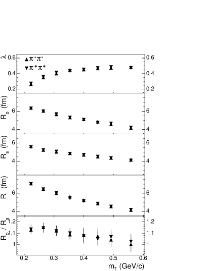
Figure 14: HBT parameters for 0–5% most central events for $\pi^{+}\pi^{+}$ and $\pi^{-}\pi^{-}$ correlation functions. Error bars include statistical and systematic uncertainties.

Figure 14 shows the HBT parameters $\lambda$, $R_{o}$, $R_{s}$, $R_{l}$ and the ratio $R_{o}/R_{s}$ for the 0–5% most central events as a function of $m_{T}$ for $\pi^{+}\pi^{+}$ and $\pi^{-}\pi^{-}$ correlation functions. We observe excellent agreement between the parameters extracted from the positively and negatively charged pion analyses. The $\lambda$ parameter increases with $m_{T}$. This is consistent with studies at lower energies ADLER01 ; BEARD98 ; LISA00 ; AGGAR00 , in which the increase was attributed to decreased contributions of pions from long-lived resonances at higher $p_{T}$. The three HBT radii rapidly decrease as a function of $m_{T}$; the decrease of the transverse radii ($R_{o}$ and $R_{s}$) with $m_{T}$ is usually attributed to the radial flow WIEDE98 ; TOMAS00 ; WIEDE96 ; the strong decrease in $R_{l}$ might be produced by the longitudinal flow WIEDE98 ; MAKHL88 ; WIEDE96 ; AKKEL95 ; HERRM95 . $R_{o}$ falls steeper than $R_{s}$ with $m_{T}$ which is consistent with $R_{o}$ being more affected by radial flow RETIE03 . In contrast to many model predictions RISCH96 ; HEINZ02 , $R_{o}/R_{s}~{}\sim~{}1$ which indicates short emission duration in a blast wave parametrization RETIE03 as will be discussed in next section.

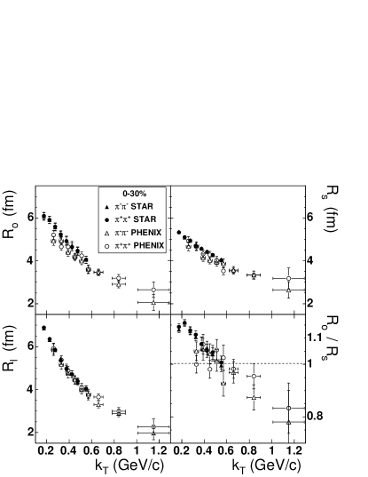
Figure 15: HBT parameters from STAR and PHENIX at the same beam energy for the 0–30% most central events. Error bars include statistical and systematic uncertainties.

Figure 15 compares our extracted HBT radius parameters from $\pi^{+}\pi^{+}$ and $\pi^{-}\pi^{-}$ correlation functions for the 0–30% most central events with those obtained by the PHENIX collaboration ADLER03 at the same beam energy and centrality. The same fitting procedure has been used in both analysis. In general, very good agreement is observed in the three radii, although small discrepancies are seen in $R_{o}$ at small $k_{T}$.

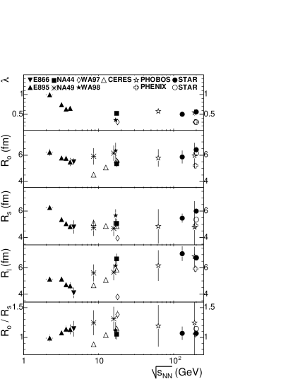
Figure 16: Energy dependence of $\pi^{-}$ HBT parameters for central Au+Au, Pb+Pb, and Pb+Au collisions at midrapidity and $\langle k_{T}\rangle~{}\approx~{}0.2$ GeV/c ADLER01 ; ADAMO03 ; BEARD98 ; LISA00 ; AGGAR00 ; ADLER03 ; SOLTZ99 ; BLUME02 ; ANTIN01 ; BACK04 . Open symbols indicate that fitting was done according to the Bowler-Sinyukov procedure (or a similar one in the case of the results from Phobos). Error bars on NA44, NA49, CERES, PHENIX, Phobos and STAR results include systematic uncertainties; error bars on other results are only statistical.

Figure 16 shows the HBT parameters vs. collision energy for midrapidity, low $p_{T}$ $\pi^{-}\pi^{-}$ from central Au+Au, Pb+Pb or Pb+Au collisions. In order to compare with our previous results at $\sqrt{s_{NN}}=130$ GeV, we applied similar cuts in our analysis as those described in ADLER01 and fit our correlation function according to the standard procedure described in section III.4 to extract the HBT parameters at $\sqrt{s_{NN}}=200$ GeV, closed circles at that energy in Fig. 16. We observe an increase of $\sim$ 10% in the transverse radii $R_{o}$ and $R_{s}$. In the case of $R_{s}$, this increase could be attributed to a larger freeze-out volume for a larger pion multiplicity. $R_{l}$ is consistent with our result at lower energy. The predicted increase by hydrodynamic models in the ratio $R_{o}/R_{s}$ as a probe of the formation of QGP is not observed at $\sqrt{s_{NN}}=200$ GeV. More discussion on the lack of energy dependence of the HBT radii and its possible relation with the constant mean free path can be found in reference ADAMO03b .

We have also included in Fig. 16 the values for the HBT parameters at $\sqrt{s_{NN}}=200$ GeV extracted when applying the cuts discussed in section II and fitting the correlation function according to the Bowler-Sinyukov procedure (section III.4), open circles in the figure. This procedure is also used by the CERES collaboration. The smaller $\lambda$, $R_{o}$, and $R_{s}$ can be explained by the different cuts as already discussed in section III.4. The larger value for $R_{o}/R_{s}$ is due to the improved procedure of taking Coulomb interaction into account in the Bowler-Sinyukov procedure, section III.4.

IV.3 Centrality dependence of the $m_{T}$ dependence

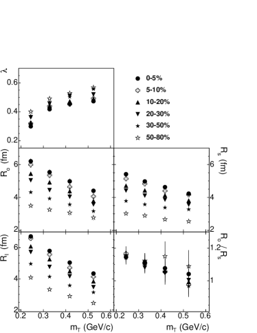
Figure 17: HBT parameters vs. $m_{T}$ for 6 different centralities. Error bars include statistical and systematic uncertainties.

We observe excellent agreement between the results for positively and negatively charged pion correlation functions for the most central collisions shown in the previous section. Therefore, we add the numerators and denominators of the correlation functions for positive and negative pions in order to improve statistics; all the results shown in the rest of this section correspond to these added correlation functions. The centrality dependence of the source parameters is presented in Fig. 17 where the HBT parameters are shown as a function of $m_{T}$ for 6 different centralities. The $\lambda$ parameter slightly increases with decreasing centrality. The three radii increase with increasing centrality and $R_{l}$ varies similar to $R_{o}$ and $R_{s}$. For $R_{o}$ and $R_{s}$ this increase may be attributed to the initial geometrical overlap of the two nuclei. $R_{o}/R_{s}~{}\sim~{}1$, for all centralities.

IV.4 Azimuthally-sensitive HBT

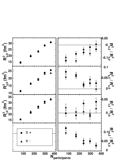
Figure 18: Fourier coefficients of azimuthal oscillations of HBT radii vs. number of participating nucleons, for $\pi^{+}$ and $\pi^{-}$ pairs separately ($0.25<k_{T}<0.35$ GeV/c). Left panels: means ($0^{\rm{th}}$-order FC) of oscillations; right panels: relative amplitudes (see text for details). Larger participant numbers correspond to more central collisions.

The results presented in ADAMS03c were for $\pi^{+}$ and $\pi^{-}$ correlation functions combined before fitting. Figure 18 shows the consistency of the Fourier coefficients obtained with Eq. (6) as a function of number of participants.

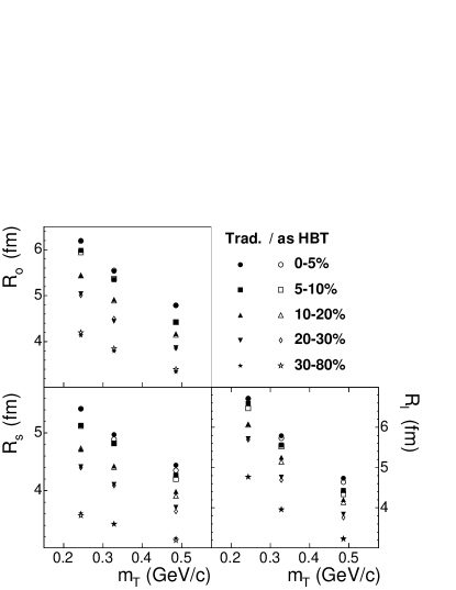
Figure 19: Comparison between the HBT radii obtained from and azimuthally integrated (traditional) HBT analysis and the $0^{\textrm{th}}$-order Fourier coefficients from an azimuthally-sensitive HBT analysis. Error bars include only statistical uncertainties.

In section III we noted that the $0^{\textrm{th}}$ order Fourier coefficients correspond to the extracted HBT radii in an azimuthally integrated analysis. This is confirmed in Fig. 19 that shows the excellent agreement between them. The azimuthally integrated (traditional) HBT radii (closed symbols) agree within 1/10 fm with the $0^{\textrm{th}}$-order Fourier coefficients (open symbols) from the azimuthally-sensitive HBT analysis.

V Discussion of results

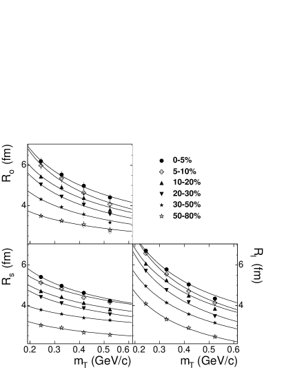
Figure 20: HBT radius parameters for 6 different centralities. The lines indicate power-law fits ($R_{i}(m_{T})~{}=~{}R_{i}^{\prime}\cdot(m_{T}/m_{\pi})^{-\alpha_{i}}$) to each parameter for each centrality.

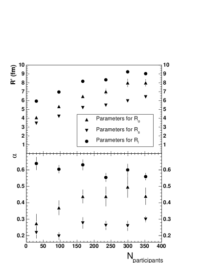
Figure 21: Extracted parameters $R^{\prime}$ in the top panel, $\alpha$ in the bottom from the power-law fits to the HBT radius parameters (lines in Fig. 20).

As already mentioned in section IV.2, the dependence of the HBT radii on the transverse mass contains dynamical information about the particle emitting source. In order to extract this information, we fit the $m_{T}$ dependence of the HBT radii for each centrality from Fig. 17 using a simple power-law fit: $R_{i}(m_{T})~{}=~{}R_{i}^{\prime}\cdot(m_{T}/m_{\pi})^{-\alpha_{i}}$ (solid lines in Fig. 20). Figure 21 shows the extracted fit parameters for the three HBT radii, $R^{\prime}$ in the top panel and $\alpha$ in the lower panel, as a function of the number of participants, where $N_{\textrm{participants}}$ has been calculated from a Glauber model described in ADAMS03b . $N_{\textrm{participants}}$ increases with the centrality of the collision. $R^{\prime}$ decreases with decreasing number of participants, which is consistent with the decreasing initial source size. $\alpha$ is approximately constant for $R_{l}$ which would indicate that the longitudinal flow is similar for all centralities. However, for the transverse radii $R_{o}$ and $R_{s}$, $\alpha$ seems to decrease for the most peripheral collisions which could be an indication of a small reduction of transverse flow and/or an increase of temperature for those most peripheral collisions. This is consistent with the values for flow and temperature extracted from blast wave fits to pion, kaon, and proton transverse momentum spectra ADAMS03 , as well as to HBT as will be discussed in next section. The drop of $\alpha$ with decreasing number of participants is faster in $R_{o}$ than in $R_{s}$ which could again indicate that $R_{o}$ might be more affected by radial flow RETIE03 .

V.1 Blast wave parametrization

Centrality (%)	$T$ (MeV)	$\rho_{0}$	$R$ (fm)	$\tau$ (fm/c)	$\Delta\tau$ (fm/c)	$\chi^{2}$/dof
0–5	97 $\pm$ 2	1.03 $\pm$ 0.01	13.3 $\pm$ 0.2	9.0 $\pm$ 0.3	2.83 $\pm$ 0.19	3.13/9
5–10	98 $\pm$ 2	1.00 $\pm$ 0.01	12.6 $\pm$ 0.2	8.7 $\pm$ 0.2	2.45 $\pm$ 0.17	2.71/9
10–20	98 $\pm$ 3	0.98 $\pm$ 0.01	11.5 $\pm$ 0.2	8.1 $\pm$ 0.2	2.35 $\pm$ 0.16	2.61/9
20–30	100 $\pm$ 2	0.94 $\pm$ 0.01	10.5 $\pm$ 0.1	7.2 $\pm$ 0.1	2.10 $\pm$ 0.09	0.99/9
30–50	108 $\pm$ 2	0.86 $\pm$ 0.01	8.8 $\pm$ 0.1	5.9 $\pm$ 0.1	1.74 $\pm$ 0.12	2.13/9
50–80	113 $\pm$ 2	0.74 $\pm$ 0.01	6.5 $\pm$ 0.1	4.0 $\pm$ 0.2	1.73 $\pm$ 0.10	1.12/9

Table 3: Extracted parameters from a blast wave fit to azimuthally integrated pion HBT radii, with $T$ and $\rho_{0}$ fixed from fits to pion, kaon, and proton transverse momentum spectra and $v_{2}$.

Cent. (%)	$T$ (MeV)	$\rho_{0}$	$\rho_{2}$	$R_{x}$ (fm)	$R_{y}$ (fm)	$\tau$ (fm/c)	$\Delta\tau$ (fm/c)	$\chi^{2}$/dof
0–5	97 $\pm$ 2	1.03 $\pm$ 0.01	0.03 $\pm$ 0.002	12.9 $\pm$ 0.1	13.4 $\pm$ 0.1	8.9 $\pm$ 0.2	3.16 $\pm$ 0.11	106.8/63
5–10	98 $\pm$ 2	1.00 $\pm$ 0.01	0.04 $\pm$ 0.002	12.1 $\pm$ 0.1	12.9 $\pm$ 0.1	8.2 $\pm$ 0.2	2.73 $\pm$ 0.12	103.2/63
10–20	98 $\pm$ 3	0.98 $\pm$ 0.01	0.05 $\pm$ 0.002	10.9 $\pm$ 0.1	11.9 $\pm$ 0.1	7.8 $\pm$ 0.2	2.59 $\pm$ 0.10	131.06/63
20–30	100 $\pm$ 1	0.94 $\pm$ 0.01	0.07 $\pm$ 0.002	9.7 $\pm$ 0.1	11.0 $\pm$ 0.1	6.9 $\pm$ 0.1	2.29 $\pm$ 0.10	87.2/63
30–80	112 $\pm$ 2	0.82 $\pm$ 0.05	0.10 $\pm$ 0.005	7.4 $\pm$ 0.1	8.7 $\pm$ 0.1	5.1 $\pm$ 0.2	1.94 $\pm$ 0.14	189.4/63

Table 4: Extracted parameters from a blast wave fit to azimuthally sensitive pion HBT radii, with $T$ and $\rho_{0}$ fixed from fits to pion, kaon, and proton transverse momentum spectra and $v_{2}$.

Hydrodynamic calculations that successfully reproduce transverse momentum spectra and elliptic flow, fail to reproduce the HBT parameters HEINZ02 . In most cases, these calculations underestimate $R_{s}$ and overestimate $R_{o}$ and $R_{l}$. Since $R_{s}$ only probes the spatial extent of the source while $R_{o}$ and $R_{l}$ are also sensitive to the system lifetime and the duration of the particle emission PRATT84 , they may be underestimating the system size and overestimating its evolution time and emission duration. We fit our data with a blast wave parametrization designed to describe the kinetic freeze-out configuration. In this section we will discuss the extracted parameters and their physical implications.

This blast wave parametrization RETIE03 assumes that the system is contained within an infinitely long cylinder along the beam line and requires longitudinal boost invariant flow. It will be shown that this latter assumption is not necessarily correct. It also assumes uniform particle density. The single set of free parameters in this parametrization is: the kinetic freeze-out temperature ($T$); the maximum flow rapidity ($\rho=\tilde{r}(\rho_{0}+\rho_{a}\cos(2\phi))$, for an azimuthally integrated analysis $\rho_{a}=0$); the radii ($R$ for the azimuthally integrated analysis and $R_{x},R_{y}$ for the azimuthally sensitive analysis) of the cylindrical system; the system longitudinal proper time ($\tau=\sqrt{t^{2}-z^{2}}$); and the emission duration ($\Delta\tau$).

We use this parametrization to fit the azimuthally integrated pion HBT radii, as well as the azimuthally sensitive pion HBT radii. In both fits, $T$ and $\rho_{0}$ are fixed to those extracted from a blast wave fit to pion, kaon and proton transverse momentum spectra ADAMS03 and $v_{2}$ ADAMS04 . By doing this, the azimuthally integrated and azimuthally sensitive radii are fitted with the same temperature and $\rho_{0}$, and the edge source radii can be compared directly. Also, a 5% error was added to all HBT radii before the fit in order to reflect the blast wave systematic errors described in RETIE03 . In the fit, the transverse flow rapidity linearly increases from zero at the center to a maximum value at the edge of the system.The best fit parameters are summarized in Table 4, for the azimuthally integrated analysis, and Table 4, for the azimuthally sensitive analysis.

Most of the parameters, as well as their evolution with centrality, agree with similar studies. Temperature decreases with increasing centrality and the average transverse flow velocity ($\langle\beta_{T}\rangle=\int\textrm{arctanh}(\rho_{0}\frac{r}{R})rdr/\int rdr$) increases with increasing centrality. Both results are consistent with those extracted from fits to spectra only ADAMS03 and reflect increased rescattering, expansion and system evolution time with increasing centrality.

Figure 22: Extracted freeze-out source radius extracted from a blast wave fit; source radius $R_{\textrm{geom}}$ from fits to $R_{s}$ (lines in Fig. 23); and $2\cdot R_{s}$ for the lowest $k_{T}$ bin as a function of number of participants. $R$ from blast wave contains only uncertainties from fit; $R_{\textrm{geom}}$ error bars contain systematic uncertainties from the input parameters; $2\cdot R_{s}$ contains the statistical and systematic uncertainties from $R_{s}$.

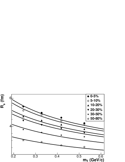
Figure 23: HBT parameter $R_{s}$. Lines represent the fits $R_{s}(m_{T})=\sqrt{R_{\textrm{geom}}^{2}/\Big{[}1+\rho_{0}^{2}(\frac{1}{2}+\frac{m_{T}}{T})\Big{]}}$.

Figure 22 shows the $R$ parameter extracted from the blast wave fit as they are in Table 4. Also shown in that plot is $R_{\textrm{geom}}$ calculated assuming a transverse expanding, longitudinally boost-invariant source, and a Gaussian transverse density profile, by fitting the $m_{T}$ dependence of $R_{s}$ to WIEDE96 :

$$R_{s}(m_{T})=\sqrt{\frac{R_{\textrm{geom}}^{2}}{1+\rho_{0}^{2}(\frac{1}{2}+\frac{m_{T}}{T})}},$$ (20)

where $T$ is the freeze-out temperature and $\rho_{0}$ is the surface transverse rapidity. Figure 23 shows such fits to $R_{s}$ for each centrality with $T$ and $\rho_{0}$ extracted from blast wave fits to pion, kaon, and proton transverse momentum spectra ($T$ = 90 MeV, $\rho_{0}$ = 1.20 for the most central collisions and $T$ = 120 MeV, $\rho_{0}$ = 0.82 for the most peripheral bins) ADAMS03 . Fig. 22 shows good agreement between these two extracted radii that increase from $\sim$ 5 fm for the most peripheral collisions to $\sim$ 13 fm for the most central collisions following the growth of the system initial size. The differences may be explained by the poor quality of the fits to $R_{s}$ as seen in Fig. 23.

As already mentioned, $R_{s}$ carries only spatial information about the source WIEDE98 ; WIEDE99 . In the special case of vanishing space-momentum correlations (no transverse flow or $T\rightarrow\infty$), the source spatial distribution may be modelled by a uniformly filled disk of radius $R$, which in this case is exactly two times $R_{s}$, the RMS of the distribution along a specific direction. In Fig. 22 we have included $2\cdot R_{s}$ for our lowest $k_{T}$ bin, $k_{T}$ = [150,250] MeV/c, in order to compare it with the extracted source radii. We observe the effect of space-momentum correlations that reduce the size of the regions of homogeneity in the results from the most central collisions for which $2\cdot R_{s}$ is smaller than the extracted radii from the fit.

Centrality	$R_{x,\textrm{initial}}$ (fm)	$R_{y,\textrm{initial}}$ (fm)
0–5%	5.70 $\pm$ 0.01	5.86 $\pm$ 0.01
5–10%	5.28 $\pm$ 0.01	5.72 $\pm$ 0.01
10–20%	4.74 $\pm$ 0.01	5.50 $\pm$ 0.01
20–30%	4.14 $\pm$ 0.01	5.12 $\pm$ 0.01
30–50%	3.58 $\pm$ 0.01	4.70 $\pm$ 0.01
50–80%	2.84 $\pm$ 0.01	4.02 $\pm$ 0.01
30–80%	3.48 $\pm$ 0.01	4.60 $\pm$ 0.01

Table 5: Initial in-plane ($R_{x,\textrm{initial}}$) and out-of-plane ($R_{y,\textrm{initial}}$) radii for 7 different centrality bins.

For an azimuthally asymmetric collision, the initial source has an elliptic shape with the larger axis perpendicular to the reaction plane (out-of-plane) and the shorter axis in the reaction plane (in-plane). In order to calculate the radii of the initial source in the $x$ (in-plane) and $y$ (out-of-plane) direction we first get the initial distribution of particles in the almond shaped initial overlap from a Monte Carlo Glauber model calculation as described in ADAMS03b . The in-plane ($R_{x,initial}$) and out-of-plane ($R_{y,initial}$) initial radii are calculated as the radii of the region that contains 95% of the particles. The values for the initial in-plane and out-of-plane edge radii are shown in Table 5. The azimuthally integrated initial radius ($R_{\textrm{initial}}$) can be calculated from those two radii as:

$$R_{\textrm{initial}}=\sqrt{\frac{R_{x,\textrm{initial}}^{2}+R_{y,\textrm{initial}}^{2}}{2}}.$$ (21)

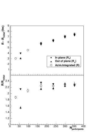
Figure 24: $R-R_{\textrm{initial}}$ (top panel) and $R/R_{\textrm{initial}}$ (bottom panel) for the azimuthally integrated analysis and in the x (in-plane) and y (out-of-plane) directions for the azimuthally-sensitive case vs. number of participants.

Figure 24 (bottom panel) shows $R/R_{\textrm{initial}}$ vs. number of participants for in-plane, out-of-plane and azimuthally integrated directions. The final source radii are those extracted from the blast wave parametrization. $R/R_{\textrm{initial}}$ is the relative expansion of the source which is stronger in-plane than out-of-plane for the most peripheral collisions, and it is similar in both directions for the most central collisions. The azimuthally integrated radius indicates a strong relative expansion of the source for central collisions. This expansion seems to be very similar for all centralities, decreasing just for the most peripheral cases. Figure 24 (top panel) shows the overall expansion of the source given by $R-R_{\textrm{initial}}$ vs. number of participants.

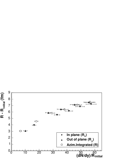
Figure 25: $R-R_{\textrm{initial}}$ for the azimuthally integrated analysis and in the x (in-plane) and y (out-of-plane) directions for the azimuthally-sensitive case vs. $(dN/dy)/R_{\textrm{initial}}$.

While the absolute expansion ($R-R_{\textrm{initial}}$) increases steadily going to more central collision, the relative expansion saturates when the number of participant reaches 150. Furthermore, both absolute and relative expansions differ significantly in peripheral events when comparing the in-plane and out-of-plane directions, while they are similar for the most central. This is expected arguing that the expansion, or in other word flow, is driven by particle reinteractions following the initial pressure gradients which in turn follow the initial energy density gradients. As the centrality increases the difference between the initial energy density gradient in-plane and out-of-plane diminishes, which brings the expansions in-plane and out-of-plane closer together.

The question is then what drives the transverse expansion. The difference between the in-plane and out-of-plane expansion at a given centrality shows that the initial energy density gradient matters. The initial energy density gradients are responsible for establishing the initial expansion velocity but the spatial expansion will also depend on for how long the system expands. The system lifetime is likely to depend on the initial energy density, which may be gauged by dividing the particle multiplicity ($dN/dy$) by the initial area estimated in the Glauber framework as done in ADAMS03b . Following this idea, we investigate how the transverse expansion evolves while varying centrality, which affects both the average energy density and the energy density gradient. We find that the transverse expansion scales with $(dN/dy)/R_{\textrm{initial}}$ as shown in Fig. 25. This figure shows $R-R_{\textrm{initial}}$ vs. $(dN/dy)/R_{\textrm{initial}}$, where $dN/dy$ is for pions as reported in ADAMS03 and $R_{\textrm{initial}}$ is the corresponding in-plane, out-of-plane or azimuthally integrated initial radius described above. This quantity scales neither as a gradient nor as an energy density but it appears to contain the relevant parameters that drive the transverse expansion. We observe a clear scaling for $R_{x}$ and $R_{y}$ as well as for the azimuthally integrated radius $R$, with $(dN/dy)/R_{\textrm{initial}}$. For the same collisions, the in-plane expansion corresponds to a higher value of $(dN/dy)/R_{\textrm{initial}}$ than the corresponding out-of-plane expansion.

The good fit to the data obtained with the blast wave parametrization, consistent with expansion, and the comparison in different ways of the initial and final sizes of the source clearly indicate that the results can be interpreted in terms of collective expansion that could be driven by the initial pressure gradient. However, the time scales extracted from the fit seem to be very small, smaller than the values predicted by hydrodynamic models.

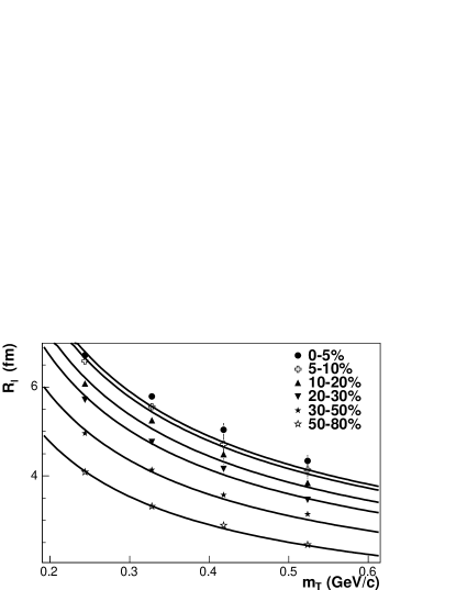
Figure 26: Longitudinal HBT radius $R_{l}$. Lines represent the fits $R_{l}=\tau\sqrt{\frac{T}{m_{T}}\frac{K_{2}(m_{T}/T)}{K_{1}(m_{T}/T)}}$ for each centrality.

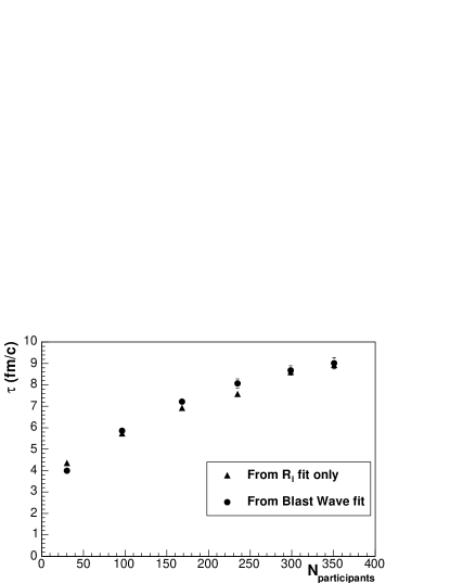
Figure 27: Evolution time $\tau$ vs. number of participants as extracted from a fit to $R_{l}$, lines in Figure 26 (triangles), and from a blast wave fit to HBT parameters and spectra (circles).

From the dependence of $R_{l}$ on $m_{T}$ shown in Fig. 26, and assuming boost-invariant longitudinal flow, we can extract information about the evolution time-scale of the source, or proper time of freeze-out, by fitting it to a formula first suggested by Sinyukov and collaborators MAKHL88 ; AKKEL95 and then improved by others RETIE03 :

$$R_{l}=\tau\sqrt{\frac{T}{m_{T}}\frac{K_{2}(m_{T}/T)}{K_{1}(m_{T}/T)}}$$ (22)

where $T$ is the freeze-out temperature and $K_{1}$ and $K_{2}$ are the modified Bessel functions of order 1 and 2. This expression for $R_{l}$ also assumes vanishing transverse flow and instantaneous freeze-out in proper time (i.e., $\Delta\tau$ = 0). The first assumption is approximatively justified by the small dependence of $R_{l}$ on $\rho_{0}$ in full calculation RETIE03 . The second approximation is justified by the small $\Delta\tau$ from blast wave fits, Table 4. Figure 26 also shows the fits to $R_{l}$ (lines) using temperatures, $T$, consistent with spectra as for the fit to $R_{s}$. The extracted values for the evolution time $\tau$ are shown in Fig. 27. The evolution time increases with centrality from $\tau\approx$ 4 fm/c for the most peripheral events to $\tau\approx$ 9 fm/c for the most central events. In the same plot, the extracted evolution time from the blast wave fit is shown. Good agreement is observed between the two extracted proper times for all centralities. They are surprisingly small as compared with hydrodynamical calculations that predict a freeze-out time of $\sim$ 15 fm/c in central collisions. These hydrodynamical calculations may over-predict the system lifetime or the assumption on which the extraction of $\tau$ is based in the blast wave parametrization, longitudinal boost invariant expansion, might not be completely justified.

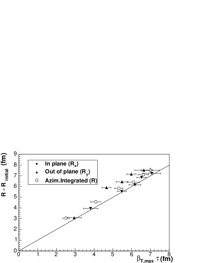
Figure 28: $R-R_{\textrm{initial}}$ for the azimuthally integrated analysis and for the in-plane and out-of-plane directions vs. $\beta_{T,\textrm{max}}\cdot\tau$. The line is a “$y=x$” line.

As a check for the consistency of the evolution time extracted from the blast wave fit, Fig. 28 shows the final source radius as extracted from the blast wave fit minus the initial source size vs. $\beta_{T,\textrm{max}}\cdot\tau$. This $\beta_{T,\textrm{max}}$ is the maximum flow velocity and is expected to be the velocity at the edge of the expanding source at kinetic freeze-out. It has been calculated from the $\rho_{0}$ and $\rho_{a}$ blast wave parameters as $\beta_{T,\textrm{max}}=\tanh(\rho_{0}+\rho_{a}\cos(2\phi))$. $\phi$ is 0 in-plane and $\pi/2$ out-of-plane RETIE03 , and $\rho_{a}$ is 0 for the azimuthally integrated analysis and is given in Table 4 for the azimuthally sensitive analysis. The evolution time, $\tau$, is the blast wave parameter shown in Fig. 27, and Table 4. The systematic errors in $\beta_{T,\textrm{max}}\cdot\tau$ come from the finite size bin in centrality. If the extracted radius and proper-time are right, the initial and final edge radii should be related by the relation $R_{\textrm{final}}~{}<~{}R_{\textrm{initial}}~{}+~{}\beta_{T,\textrm{max}}\cdot\tau$ so that the points in the figure should all be clearly below the solid line ($\beta_{T,\textrm{max}}\cdot\tau~{}=~{}R-R_{\textrm{initial}}$). Since most points are above the line, a possible explanation is that $\tau$ is not properly calculated within the blast wave parametrization. A larger $\tau$ would move the points below the line.

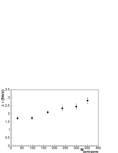
Figure 29: Emission duration time $\Delta\tau$ vs. number of participants as extracted using a blast fit to HBT parameters and spectra.

Figure 29 shows the emission duration time, $\Delta\tau$ as a function of number of participants. $\Delta\tau$ increases with increasing centrality up to $\sim$ 3 fm/c. It is relatively small for all centralities, however it has increased with respect to the values extracted from our analysis at $\sqrt{s_{NN}}$ = 130 GeV RETIE03 due to the improved procedure of taking Coulomb interaction into account and the consequent increase in $R_{o}$.

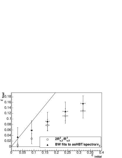
Figure 30: Final source eccentricity ($\varepsilon_{\textrm{final}}$) as calculated from the Fourier coefficients ($2R_{s,2}^{2}/R_{s,0}^{2}$) and from the final in-plane and out-of-plane radii ($(R_{y}^{2}-R_{x}^{2})/(R_{y}^{2}+R_{x}^{2})$) vs. initial eccentricity ($\varepsilon_{\textrm{initial}}$). The most peripheral collisions correspond to the largest eccentricity. The line indicates $\varepsilon_{\textrm{final}}=\varepsilon_{\textrm{initial}}$. Systematic errors of 30%, based on sensitivity to model parameters RETIE03 , are assigned to $\varepsilon_{\textrm{final}}$ extracted from the Fourier coefficients.

The freeze-out shape of the source in non-central collisions and its relation to the spatial anisotropy of the collision’s initial overlap region give us another hint about the system lifetime. The initial anisotropic collision geometry generates greater transverse pressure gradients in the reaction plane than perpendicular to it. This leads to a preferential in-plane expansion KOLB00 ; VOLOS03 ; ADLER01b which diminishes the initial anisotropy. A long-$\tau$ source would be less out-of-plane extended and perhaps in-plane extended. The eccentricity of the initial overlap region has been calculated from the initial RMS of the distribution of particles, as given by the Monte Carlo Glauber calculation, in the in-plane and out-of-plane directions as:

$$\varepsilon=\frac{(R_{y,\textrm{initial}}^{\textrm{RMS}})^{2}-(R_{x,\textrm{initial}}^{\textrm{RMS}})^{2}}{(R_{y,\textrm{initial}}^{\textrm{RMS}})^{2}+(R_{x,\textrm{initial}}^{\textrm{RMS}})^{2}}.$$ (23)

Figure 30 shows the relation between initial and final eccentricities, with more peripheral collisions showing a larger final anisotropy. The final source eccentricity has been calculated from the Fourier coefficients ($2R_{s,2}^{2}/R_{s,0}^{2}$), as well as from the final in-plane and out-of-plane radii ($(R_{y}^{2}-R_{x}^{2})/(R_{y}^{2}+R_{x}^{2})$) extracted from the blast wave fit to azimuthally sensitive HBT and spectra described above. The source at freeze-out remains out-of-plane extended indicating that the outward pressure and/or expansion time was not sufficient to quench or reverse the initial spatial anisotropy. The large elliptic flow and small HBT radii observed at RHIC energies might favor a large pressure build-up in a short-lived system compared to hydrodynamic calculations. Also, out-of-plane freeze-out shapes tend to disfavor a long-lived hadronic rescattering phase following hydrodynamic expansion TEANE01 . This short hadronic phase is consistent with a short emission time.

VI Conclusion

We have presented a detailed description of a systematic HBT analysis in Au+Au collisions at $\sqrt{s_{NN}}$ = 200 GeV. We have analyzed the Gaussianess of the correlation function and conclude that there is a deviation from a pure Gaussian, however it is not clear how this affects the HBT parameters, extracted assuming a Gaussian, that will be compared to models. We have studied the centrality dependence of the $k_{T}$ dependence of the HBT parameters and extracted geometrical and dynamical information on the source at freeze-out. We conclude that there is a significant expansion in Au+Au collisions, and that the relative expansion does not significantly depend on centrality. The system expands by a factor of at least 2.0 for most centralities. This is well established by HBT. The initial pressure gradient seems to be driving the expansion. The extracted time scales from a blast wave fit are small. The blast wave evolution time $\tau$ is small as compared with hydrodynamical calculations which could suggest that the longitudinal boost invariant assumption has only limited validity.

We thank the RHIC Operations Group and RCF at BNL, and the NERSC Center at LBNL for their support. This work was supported in part by the HENP Divisions of the Office of Science of the U.S. DOE; the U.S. NSF; the BMBF of Germany; IN2P3, RA, RPL, and EMN of France; EPSRC of the United Kingdom; FAPESP of Brazil; the Russian Ministry of Science and Technology; the Ministry of Education and the NNSFC of China; Grant Agency of the Czech Republic, FOM and UU of the Netherlands, DAE, DST, and CSIR of the Government of India; Swiss NSF; and the Polish State Committee for Scientific Research.

References

- (1) R. Hanbury-Brown and R. Q. Twiss, Nature 178, 1046 (1956).
- (2) G. Goldhaber et al., Phys. Rev. 120, 300 (1960).
- (3) W. Bauer, C. K. Gelbke and S. Pratt, Annu. Rev. Nucl. Part. Sci. 42, 77 (1992).
- (4) U. Heinz and B. V. Jacak, Ann. Rev. Nucl. Sci. 49, 529 (1999).
- (5) S. Pratt, Phys. Rev. Lett. 53, 1219 (1984).
- (6) A. N. Makhlin and Y. M. Sinyukov, Z. Phys. C39, 69 (1988).
- (7) S. A. Voloshin and W. E. Cleland, Phys. Rev. C53, 896 (1996).
- (8) S. A. Voloshin and W. E. Cleland, Phys. Rev. C54, 3212 (1996).
- (9) U. Heinz, A. Hummel, M. A. Lisa, U. A. Wiedemann, Phys. Rev. C66, 044903 (2002).
- (10) C. Adler et al. (STAR Collaboration), Phys. Rev. Lett. 87, 082301 (2001).
- (11) K. Adcox et al. (PHENIX Collaboration), Phys. Rev. Lett. 88, 242301 (2002).
- (12) D. H. Rischke and M. Gyulassy, Nucl. Phys. A608, 479 (1996).
- (13) D. H. Rischke, Nucl. Phys. A610, 88c (1996).
- (14) P. F. Kolb and U. Heinz, nucl-th/0305084.
- (15) T. Hirano, nucl-th/0403042.
- (16) Z-W. Lin, C. M. Ko and S. Pal, Phys. Rev. Lett. 89, 152301 (2002).
- (17) The multistage AMPT model reproduces flow with mb ZWLIN02b , after non-flow effects are removed from the data ZWLIN02 . HBT projections are reproduced, however, only when mb. We thank Z-W. Lin from bringing this to our attention.
- (18) J. Y. Ollitrault, Phys. Rev. D46, 229 (1992).
- (19) P. F. Kolb, J. Sollfrank and U. Heinz, Phys. Rev. C62, 054909 (2000).
- (20) C. Adler et al. (STAR Collaboration), Phys. Rev. Lett. 87, 182301 (2001).
- (21) S. A. Voloshin, Nucl. Phys. A715, 379c (2003).
- (22) P. F. Kolb and U. Heinz, Nucl. Phys. A715, 653 (2003).
- (23) D. Teaney, J. Lauret and E. Shuryak, nucl-th/0110037.
- (24) M. López Noriega, Ph.D. Thesis, Ohio State University (2004).
- (25) M. Anderson et al., Nucl. Instrum. Meth. A499, 659 (2003).
- (26) W. Blum and L. Rolandi. Particle Detection with drift chambers. Springer-Verlag (1993).
- (27) G. I. Kopylov, Sov. J. Nucl. Phys. 25, 578 (1977).
- (28) G. F. Bertsch, M. Gong and M. Tohyama, Phys. Rev. C37, 1428 (1998).
- (29) S. Pratt, Phys. Rev. D33, 1314 (1986).
- (30) S. Chapman, P. Scotto and U. W. Heinz, Phys. Rev. Lett. 74, 4400 (1005).
- (31) J. Adams et al. (STAR Collaboration), Phys. Rev. Lett. 91, 262301 (2003).
- (32) U. A. Wiedemann, Phys. Rev. C57, 266 (1998).
- (33) U. A. Wiedemann and U. Heinz, Phys. Rept. 319, 145 (1999).
- (34) S. Pratt, Phys. Rev. D33, 72 (1986).
- (35) L. Ahle et al. (E802 Collaboration), Phys. Rev. C66, 054906 (2002).
- (36) We thank H. Appelshäuser for explaining this to us.
- (37) M. G. Bowler, Phys. Lett. B270, 69 (1991).
- (38) Yu. M. Sinyukov et al., Phys. Lett. B432, 249 (1998).
- (39) D. Adamova et al. (CERES Collaboration), Nucl. Phys. A714, 124 (2003).
- (40) R. Lednicky and V. L. Lyuboshitz, Yad. Fiz 35, 1316 (1982) [Sov. J. Nucl. Phys. 35, 770 (1982)]. Fortran program provided by R. Lednicky.
- (41) M. G. Bowler, Z. Phys. C39, 81 (1988).
- (42) W. A. Zajc, Phys. Rev. C29, 2173 (1984).
- (43) H. W. Barz, Phys. Rev. C59, 2214 (1999).
- (44) J. Adams et al. (STAR Collaboration), Phys. Rev. Lett. 93, 012301 (2004).
- (45) K. Ackermann et al. (STAR Collaboration), Phys. Rev. Lett. 86, 402 (2001).
- (46) S. Voloshin and Y. Zhang, Z. Phys. C70, 665 (1996).
- (47) A. M. Poskanzer and S. A. Voloshin, Phys. Rev. C58, 1671 (1998).
- (48) T. Csörgő and A. T. Szerzo, hep-ph/9912220.
- (49) T. Csörgő and S. Hegyi, Phys. Lett. B489, 15 (2000).
- (50) T. Csörgő, S. Hegyi and W. A. Zajc, nucl-th/0310042.
- (51) B. Tomasik, U. A. Wiedemann, U. Heinz, Nucl. Phys. A663, 753 (2000).
- (52) U. Wiedemann, P. Scotto and U. Heinz, Phys. Rev. C53, 918 (1996).
- (53) I. G. Bearden et al. (NA44 Collaboration), Phys. Rev. C58, 1656 (1998).
- (54) M. A. Lisa et al. (E895 Collaboration), Phys. Rev. Lett. 84, 2798 (2000).
- (55) M. M. Aggarwal et al. (WA98 Collaboration), Eur. Phys. J. C. 16, 445 (2000).
- (56) S. V. Akkelin and Yu. M. Sinyukov, Phys. Lett. B356, 525 (1995).
- (57) M. Herrmann and G. F. Bertsch, Phys. Rev. C51, 328 (1995).
- (58) F. Retière and M. A. Lisa, Phys. Rev. C70, 044907 (2004).
- (59) U. Heinz and P. F. Kolb, hep-ph/0204061.
- (60) S. S. Adler et al. (PHENIX Collaboration), Phys. Rev. Lett. 93, 152302 (2004).
- (61) R. Soltz et al. (E866 Collaboration), Nucl. Phys. A661, 448c (1999).
- (62) C. Blume et al. (NA49 Collaboration), Nucl. Phys. A698, 104 (2002).
- (63) F. Antinori et al. (WA97 Collaboration), J. Phys. G27, 2325 (2001).
- (64) B.B. Back et al. (Phobos Collaboration), submitted to Phys. Rev. C., nucl-ex/0409001.
- (65) D. Adamova et al. (CERES Collaboration), Phys. Rev. Lett. 90, 022301 (2003).
- (66) J. Adams et al. (STAR Collaboration), submitted to Phys. Rev. C., nucl-ex/0311017.
- (67) J. Adams et al. (STAR Collaboration), Phys. Rev. Lett. 92, 112301 (2004).
- (68) J. Adams et al. (STAR Collaboration), submitted to Phys. Rev. C., nucl-ex/0409033.
- (69) Z-W. Lin, C. M. Ko, Phys. Rev. C 65, 034904 (2002).