Azimuthal anisotropy in Au+Au collisions at $\mbox{$\sqrt{s_{\mathrm{NN}}}$}=200$ GeV

Abstract

The results from the STAR Collaboration on directed flow ($v_{1}$), elliptic flow ($v_{2}$), and the fourth harmonic ($v_{4}$) in the anisotropic azimuthal distribution of particles from Au+Au collisions at $\mbox{$\sqrt{s_{\mathrm{NN}}}$}=200$ GeV are summarized and compared with results from other experiments and theoretical models. Results for identified particles are presented and fit with a Blast Wave model. Different anisotropic flow analysis methods are compared and nonflow effects are extracted from the data. For $v_{2}$, scaling with the number of constituent quarks and parton coalescence is discussed. For $v_{4}$, scaling with $v_{2}^{2}$ and quark coalescence is discussed.

I Introduction

In heavy-ion collisions at the Relativistic Heavy Ion Collider (RHIC), the initial spatially-anisotropic participant zone evolves, via possible novel phases of nuclear matter, into the observed final state, consisting of large numbers of produced particles with anisotropic momentum distributions in the transverse plane. Important insights into the evolution may be obtained from the study of this azimuthal anisotropy, most of which is believed to originate at the early stages of the collision process. Unlike at lower beam energies review , the measured anisotropies at RHIC reach the large values predicted by hydrodynamic models and conform to the particle mass dependence expected from hydrodynamics in the kinematic region where this type of model is expected to be applicable, i.e., for transverse momenta below a couple of $\mathrm{GeV}/c$ anonQM04 . The large observed anisotropy at RHIC is argued to be indicative of early local thermal equilibrium, and the particle mass dependence is highly relevant to interpretations involving a strongly interacting Quark Gluon Plasma phase anonQM04 ; RikenWSmay04 ; miklos . At larger transverse momenta, measurements of azimuthal anisotropy are also relevant to the observation of jet quenching STARchargedhighpt ; STARhighPtV2Corr . Given the current debate around these interpretations, we summarize STAR’s findings to date in the area of azimuthal anisotropy, present additional results for identified particles, compare in detail the different analysis methods and their systematic uncertainties, compare the data to various models, and systematize the results with fits to the hydrodynamic motivated Blast Wave model.

The paper is organized into sections on the Experiment, Methods of Analysis, Results, comparison of analysis methods, comparison of results to various models, and Conclusions. The Methods Comparisons section is rather technical, dealing with systematic errors, nonflow effects, and fluctuations.

II Experiment

Table 1: Cuts used in the TPC analysis of Au+Au collisions at $\mbox{$\sqrt{s_{\mathrm{NN}}}$}=200$ GeV. Vertex refers to the event vertex, fit points are the space points on a track, and dca is the distance of closest approach of the track to the event vertex.

cut	value
$p_{t}$	0.15 to 2.0 $\mathrm{GeV}/c$
$\eta$	–1.3 to 1.3
multiplicity	$\ >\$10
vertex z	–25. to 25. cm
vertex x, y	–1.0 to 1.0 cm
fit points	$\ >\$15
fit pts / max. pts	$\ >\$0.52
dca	$\ <\$2.0 cm
trigger	min. bias

The main detectors of the STAR experiment used in these analyses are the Time Projection Chamber (TPC) STARTPC and the Forward TPCs (FTPCs) STARFTPC . The Ring Imaging Cherenkov detector (RICH) STARRICH of the STAR-RICH collaboration is also used for particle identification. The cuts on the data for most of the TPC analyses are described in Table 1, except for the upper $p_{t}$ cutoff which often goes higher as shown in the graphs. For the FTPCs the pseudorapidity acceptance is $2.4\mbox{$\ <\ $}|\eta|\mbox{$\ <\ $}4.2$, only at least 5 hits are required, the distance of closest approach of the track to the vertex (dca) is restricted to less than 3 cm, and for the $v_{1}$ analysis the vertex z is opened up to $\pm 50$ cm. The RICH detector STARRICH covers $|\eta|\mbox{$\ <\ $}0.30$ with a $20^{\circ}$ bite in azimuth. The RICH detector separates charged mesons from protons + anti-protons identified track by track. The admixture of baryons in the meson sample is always less than 10%. The momenta of the particles identified in the RICH come from tracking in the TPC.

Table 2: Listed for $\mbox{$\sqrt{s_{\mathrm{NN}}}$}=200$ GeV for each centrality bin are the range of the % most central of the hadronic cross section and its mean value, the mean charged particle multiplicity with its standard deviation spread, the estimated mean number of wounded nucleons, the estimated mean number of binary collisions, and the estimated mean impact parameter, with the uncertainties in these quantities.

Centrality bin	1	2	3	4	5	6	7	8	9
% most central	70 – 80	60 – 70	50 – 60	40 – 50	30 – 40	20 – 30	10 – 20	5 – 10	0 – 5
$\left\langle centrality\right\rangle(\%$)	73.8	64.1	53.9	44.7	35.2	25.4	15.1	7.7	2.3
$\left\langle M\right\rangle\pm\sigma$	38$\pm$11	76$\pm$17	134$\pm$24	214$\pm$32	323$\pm$42	468$\pm$53	651$\pm$64	819$\pm$48	961$\pm$56
$\left\langle N_{WN}\right\rangle\pm\sigma$	13$\pm$4	26$\pm$7	46$\pm$9	75$\pm$11	114$\pm$12	165$\pm$12	232$\pm$10	298$\pm$10	352$\pm$6
$\left\langle N_{binary}\right\rangle\pm\sigma$	11$\pm$5	28$\pm$10	61$\pm$17	120$\pm$28	216$\pm$38	364$\pm$51	587$\pm$61	825$\pm$72	1049$\pm$72
$\left\langle b\right\rangle\pm\sigma$ (fm)	13.2$\pm$0.6	12.3$\pm$0.6	11.3$\pm$0.6	10.2$\pm$0.5	9.0$\pm$0.5	7.6$\pm$0.4	5.9$\pm$0.3	4.2$\pm$0.3	2.3$\pm$0.2

The data were collected with a minimum bias trigger which required a coincidence from the two Zero Degree Calorimeters, with each signal being greater than 1/4 of the single neutron peak and arriving within a time window centered for the interaction diamond. The centrality definition, which is based on the raw charged particle TPC multiplicity with $|\eta|\mbox{$\ <\ $}0.5$, is the same as used previously centrality . The centrality bins are specified in Table 2. The mean charged particle multiplicity given in the Table 2 is for the cuts in Table 1. The estimated values in the Table come from a Monte Carlo Glauber model calculation Miller . In this calculation, the number of participants is equal to the number of wounded nucleons. The estimated errors shown for the calculated quantities come from a linear combination of the changes in the quantities caused by reasonable variations in the parameters of the model. Minimum bias refers to 0 to 80% most central hadronic cross section. Two million events are analyzed for this paper. For the analysis involving FTPCs only 70 thousand events are available. Errors presented for the data are statistical. Systematic errors are mainly due to the method of analysis, nonflow effects, and fluctuations; these will be discussed in Sec. V on Methods Comparisons.

Several methods are used to identify particles. The energy loss in the gas of the TPC identifies particles at low $p_{t}$. For this the probability PID method STARPID ; TangThesis is used requiring 95% particle purity unless otherwise stated. In the FTPCs the energy loss is not sufficient for good particle identification. The RICH detector can separate mesons from baryons up to higher $p_{t}$. Using the characteristic kink decay of $\mathrm{K}^{0}_{S}$ , one is able to go to higher $p_{t}$. Strange particles up to high $p_{t}$ are identified by their topological decay.

For the kink analysis of charged kaons, flow parameters were measured for particles that decay in flight within a fiducial volume in the TPC. The one-prong decay vertex (“kink”) provides topological identification of the particle species with good rejection of background kinkMethod . The main sources of possible misidentification are pion decays, random combinatoric background, and secondary hadronic interactions in the TPC gas. The level of background in the analyzed sample was estimated to be 5–10% but is $p_{t}$-dependent. Several cuts were applied to the raw signal in order to remove most of the background. Pion decays were removed by applying a momentum-dependent decay angle cut, which exploits differences in the decay kinematics. Other cuts were also applied to the $dE/dx$, pseudorapidity, and invariant mass of the parent track candidate, to the daughter momentum, and to the distance of closest approach associated with the two track segments at the kink vertex. Finally, there was a quality cut to remove candidates with vertices inside the TPC sector gaps where spurious kink vertices can arise kinkMethod . Currently the kink method can reconstruct charged kaons up to $p_{t}\sim 4$ GeV$/c$. The tracking software has difficulty resolving a kink vertex when the decay angle is less than about $6^{\circ}$. For kaons with $p_{t}\mbox{$\ >\ $}3$ $\mathrm{GeV}/c$, the decay angle is almost always around $6^{\circ}$ or less, so efficiency falls off rapidly above 3 GeV$/c$. The efficiency also suffers from the limited fiducial volume; the kaon must decay inside a small sub-volume of the TPC in order to provide adequate track length for both parent and daughter tracks.

Other strange particles were identified by their decay topology STARstrange ; STARspectra130 . These methods used for the strange particle decays have already been described STARstrange ; STARmultistrange .

III Methods of analysis

Directed and elliptic flow are defined as the first, $v_{1}$, and second, $v_{2}$, harmonics in the Fourier expansion of the particle azimuthal anisotropic distribution with respect to the reaction plane. The reaction plane contains the collision impact parameter. However, normally measurements are made relative to the observed event plane, and are corrected for the resolution of the event plane relative to the reaction plane. The event plane angle is defined for each harmonic, $n$, by the angle, $\Psi_{n}$, of the flow vector, $Q$, whose x and y components are given by

$$Q_{n}\cos(n\Psi_{n})=\sum[w_{i}\cos(n\phi_{i})]$$ (1)

$$Q_{n}\sin(n\Psi_{n})=\sum[w_{i}\sin(n\phi_{i})],$$

where the $\phi_{i}$ are the azimuthal angles of all the particles used to define the event plane and the weights, $w_{i}$, are used to optimize the event plane resolution. In this paper the weights for the even harmonics have been taken to be proportional to $p_{t}$ up to 2 $\mathrm{GeV}/c$ and constant above that. For the odd harmonics they have been taken to be proportional to $\eta$ for $|\eta|>1$.

STAR has previously presented results using different methods of analysis. In the standard method methods , denoted by $v_{n}$, particles are correlated with an event plane of the same harmonic. Using this method STAR has presented results on elliptic flow ($v_{2}$) for charged hadrons STARcharged ; STARchargedhighpt , identified particles STARPID , strange particles STARstrange ; STAR_Rcp , and multi-strange baryons STARmultistrange . In the $N$-particle cumulant method cumulants , denoted by $v_{n}\{N\}$, $N$-particle correlations are calculated and nonflow effects subtracted to first order when $N$ is greater than 2. Nonflow effects which affect $v_{n}$ are particle correlations which are not correlated with the reaction plane. Two-particle cumulants should give essentially the same results and errors as the standard method, but multi-particle cumulants have larger statistical errors. STAR has presented four-particle cumulant results STARcumulants for charged hadrons. In three-particle mixed harmonic methods relative to the second harmonic event plane, denoted by $v_{n}\{\mathrm{EP}_{2}\}$ when $n\neq 2$, the particles of a different harmonic are correlated with the well-determined second harmonic event plane. With mixed harmonics, nonflow effects are greatly suppressed. With this method STAR has reported results on directed flow ($v_{1}$) STARv1v4 ; STARv1 ; FTPC and higher harmonics ($v_{4}$) STARv1v4 ; STARv4 for charged hadrons.

III.1 Directed flow methods

Because directed flow goes to zero at midrapidity by symmetry, the first harmonic event plane is poorly defined in the TPC. A better way to measure $v_{1}$ is to use mixed harmonics involving the second harmonic event plane; this also suppresses nonflow contributions at the same time. One such method is the three particle cumulant method which has been described v13 .

We also measure $v_{1}$ using another mixed harmonic technique: we determine two first order reaction planes $\Psi_{1}^{\mathrm{FTPC_{1}}}$ and $\Psi_{1}^{\mathrm{FTPC_{2}}}$ in the FTPCs and the second order reaction plane $\Psi_{2}^{\mathrm{TPC}}$ in the TPC. Using the recently proposed notation (see STARv1v4 ) we denote this measurement as $v_{1}\!\left\{\mathrm{EP}_{1},\mathrm{EP}_{2}\right\}$.

$$v_{1}\{\mathrm{EP}_{1},\mathrm{EP}_{2}\}=$$ (2)

$$\frac{\left\langle\cos\left(\phi+\Psi_{1}^{\mathrm{FTPC}}-2\Psi_{2}^{\mathrm{TPC}}\right)\right\rangle}{\sqrt{\left\langle\cos\left(\Psi_{1}^{\mathrm{FTPC}_{1}}+\Psi_{1}^{\mathrm{FTPC}_{2}}-2\Psi_{2}^{\mathrm{TPC}}\right)\right\rangle\cdot\mathrm{Res}(\Psi_{2}^{\mathrm{TPC}})}},$$

where the $\phi$ of the particle is correlated with the $\Psi_{1}^{\mathrm{FTPC}}$ in the other subevent, and

$$\mathrm{Res}(\Psi_{2}^{\mathrm{TPC}})=\langle\cos[2(\Psi_{2}-\Psi_{\mathrm{RP}})]\rangle$$ (3)

represents the resolution of the second order event plane measured in the TPC. This resolution, as usual, is derived from the square-root of the correlation of TPC subevent planes. For the derivation of Eq. (2) see Appendix B.

This new $v_{1}$ method also provides an elegant tool to determine the sign of $v_{2}$. One of the quantities involved in the above measurement of $v_{1}\!\left\{\mathrm{EP}_{1},\mathrm{EP}_{2}\right\}$ (see Appendix B, Eq. (26) and compare to methods , Eq. (18)) is approximately proportional to the product of integrated values of $v_{1}^{2}$ and $v_{2}$. Applying factors for weights and multiplicities methods leads to

$$v_{1}^{2}\cdot v_{2}\approx\left(\frac{4}{\pi}\right)^{\frac{3}{2}}\sqrt{\prod_{d}\frac{1}{M_{d}}\frac{\langle w_{d}^{2}\rangle}{\langle w_{d}\rangle^{2}}}$$ (4)

$$\times\left\langle\cos\left(\Psi_{1}^{\mathrm{FTPC}_{1}}+\Psi_{1}^{\mathrm{FTPC}_{2}}-2\Psi_{2}^{\mathrm{TPC}}\right)\right\rangle,$$

where the index $d$ represents the three detectors used in the analysis: $\mathrm{FTPC}_{1}$, $\mathrm{FTPC}_{2}$, and $\mathrm{TPC}$. For each centrality class $M_{d}$ denotes the corresponding multiplicities and $w_{d}$ are the applied weights ($\eta$-weighting for $\Psi_{1}$ and $p_{T}$-weighting for $\Psi_{2}$).

III.2 Elliptic flow methods

The standard method methods correlates each particle with the event plane determined from the full event minus the particle of interest. Since the event plane is only an approximation to the true reaction plane, one has to correct for this smearing by dividing the observed correlation by the event plane resolution, which is the correlation of the event plane with the reaction plane. The event plane resolution is always less than one, and thus dividing by it raises the flow values. To make this correction the full event is divided up into two subevents (a,b), and the square root of the correlation of the subevent planes is the subevent plane resolution. The full event plane resolution is then obtained using the equations in Ref. methods which describe the variation of the resolution with multiplicity.

The scalar product method STARcumulants is a simpler variation of this method which weights events with the magnitude of the flow vector $Q$:

$$v_{n}(\eta,p_{t})=\frac{\langle Q_{n}u_{n,i}^{*}(\eta,p_{t})\rangle}{2\sqrt{\langle Q^{a}_{n}{Q^{b}_{n}}^{*}\rangle}}\,,$$ (5)

where $u_{n,i}=\cos(n\phi_{i})+i\sin(n\phi_{i})$ is the unit vector of the $i^{th}$ particle. If $Q_{n}$ is replaced by its unit vector, the above reduces to the standard method. Taking into account the non-flow contribution, the numerator of Eq. (5) can be written as STARcumulants ; STARhighPtV2Corr :

$$\langle\sum_{i}\cos 2(\phi_{p_{t}}-\phi_{i})\rangle=M\,v_{2}(p_{t})\,\bar{v}_{2}+\{\text{non-flow}\}$$ (6)

where $\phi_{p_{t}}$ is the azimuthal angle of the particle from a given $p_{t}$ bin. The first term in the r.h.s. of Eq. (6) represents the elliptic flow contribution, where $v_{2}(p_{t})$ is the elliptic flow of particles with a given $p_{t}$, and $\bar{v}_{2}$ is the average flow of particles used in the sum; $M$ is the multiplicity of particles contributing to the sum, which in this paper is performed over particles in the region $0.15\mbox{$\ <\ $}p_{t}\mbox{$\ <\ $}2.0\ \mbox{$\mathrm{GeV}/c$}$ and $|\eta|\mbox{$\ <\ $}1.0$.

The cumulant method has been well described cumulants ; cumuPraticeGuide and previously used for the analysis of STAR data STARcumulants .

To reduce the nonflow effects from intra-jet correlations at high transverse momentum, we also use a modified event plane reconstruction algorithm, where all subevent particles in a pseudorapidity region of $|\Delta\eta|\mbox{$\ <\ $}$ 0.5 around the highest $p_{t}$ particle in the event are excluded from the event plane determination. With this modified event plane method, the full event plane resolution is 15–20% worse than with the standard method due to the smaller number of tracks used for the event plane determination.

III.3 Higher harmonic methods

Since the second harmonic event plane is determined so well, one can try to determine the higher even harmonics of the azimuthal anisotropy by correlating particles with the second harmonic event plane. However, then the event plane resolution is worse because of the various possible orientations of the higher harmonics relative to the second harmonic event plane. Taking $k$ to be the ratio of the higher harmonic number to the event plane harmonic number, and using the equations in Ref. methods we obtain the resolutions in Fig. 1 for $v_{k2}\{\mathrm{EP}_{2}\}$. This method works when the resolution of the standard method ($k=1$) is large and therefore those for the higher harmonics are not too low. Also, these $k\neq 1$ methods use mixed harmonics, which involve multiparticle correlations, greatly reducing the nonflow contributions.

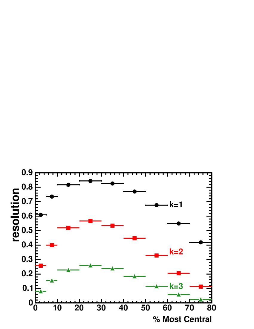
Figure 1: (color online). The event plane resolutions as a function of centrality for $v_{k2}\{\mathrm{EP}_{2}\}$.

The cumulant method with mixed harmonics has also been used for $v_{4}$ STARv1v4 .

IV Results

In the following sections we present results for directed flow, elliptic flow, and the higher harmonics. Some of the graphs have model calculations on them which will be discussed in Sec. VI. The tables of data for this paper are available at http://www.star.bnl.gov/central/publications/ .

IV.1 Directed flow, $v_{1}\!\left\{\mathrm{EP}_{1},\mathrm{EP}_{2}\right\}$

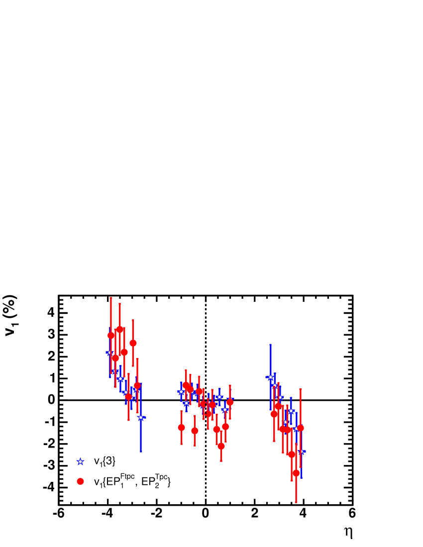
Figure 2: (color online). Directed flow of charged hadrons as a function of pseudorapidity. The measurements of $v_{1}\!\left\{\mathrm{EP}_{1},\mathrm{EP}_{2}\right\}$ (circles; centrality 20–60%) agree with the published results of $v_{1}\{3\}$ (stars; centrality 10–70%).

The STAR TPC has very good capabilities to measure elliptic flow at mid-rapidity, while the FTPCs allow one to measure directed flow. Figure 2 plots directed flow as a function of pseudorapidity, showing that $v_{1}$ appears to be close to zero near mid-rapidity. First, the analysis was done successfully on simulated data containing a fixed $v_{1}$. For real data, using random subevents in the two FTPCs to determine $\Psi_{1}^{\mathrm{FTPC}_{1}}$ and $\Psi_{1}^{\mathrm{FTPC}_{2}}$ in Eq. (2), the results are in agreement with the published measurements obtained by the three-particle cumulant method $v_{1}\{3\}$ STARv1v4 ; STARv1 , as shown in Fig. 2. Recently, PHOBOS has also reported PHOBOSQM04 $v_{1}$ values using a two-particle correlation method. While we approximately agree at $\eta=4.0$, they have finite values at $\eta=$ 2.5–3.0, while ours are close to zero, as can be seen for ours in Fig. 2.

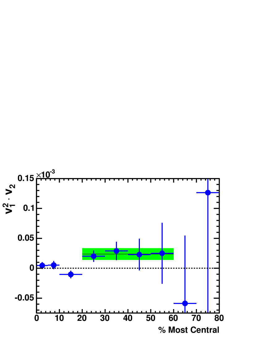
Figure 3: (color online). The product of $v_{1}^{2}$ and $v_{2}$. The shaded band is the mean value of this quantity with its error, averaged over centralities 20–60%. Since this quantity is positive, elliptic flow is measured to be in-plane.

The sign of $v_{2}$ determines whether the elliptic flow is in-plane or out-of-plane. Although the sign of $v_{2}$ had been determined to be positive from three particle correlations STARv1v4 , the above new method for $v_{1}$ allows another method based on the sign of $v_{1}^{2}\cdot v_{2}$. Since $v_{1}^{2}$ is always positive, the sign of $v_{1}^{2}\cdot v_{2}$ determines the sign of $v_{2}$.

Averaged over centralities 20–60% we measure $v_{1}^{2}\cdot v_{2}$ in Fig. 3 to be $(2.38\pm 0.99)\cdot 10^{-5}$. This is only a 2.4 sigma effect and if 10% systematic errors are assumed based on Sec. V for both $v_{1}$ and $v_{2}$ this becomes a 2.2 sigma effect. Only the mid-centrality bins are averaged because in this centrality region the expected nonflow contributions are much smaller than for the more central and peripheral bins. Therefore, with these caveats, the sign of $v_{2}$ is confirmed to be positive: in-plane elliptic flow.

IV.2 Elliptic flow, $v_{2}$

There have been many elliptic flow results from RHIC. STAR has extensive systematics which we will present and compare to the other experiments. Many of the graphs will contain Blast Wave model fits which will be discussed in Sec. VI.4 in Model Comparisons. We will present data separately for the central rapidity region, the forward region, and for high $p_{t}$.

IV.2.1 The central region

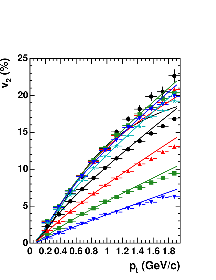
Figure 4: (color online). Charged hadron $v_{2}$ vs. $p_{t}$ for the centrality bins (bottom to top) 5 to 10% and in steps of 10% starting at 10, 20, 30, 40, 50, 60, and 70 up to 80%. The solid lines are Blast Wave fits.

The $v_{2}(p_{t})$ values for charged hadrons for individual centralities are shown in Fig. 4 with Blast Wave fits performed assuming that all charged hadrons have the mass of the pion. The data are well reproduced by the Blast Wave parameterization when $p_{t}$ is below 1 $\mathrm{GeV}/c$. Above this limit, the contribution of protons in the charged hadron sample becomes significant and changes with centrality, which challenges the pion mass assumption. Furthermore it has been found that hydrodynamic flow may not be applicable above 1 $\mathrm{GeV}/c$, especially for light particles, as new phenomena such as hadronization by recombination may become significant reco .

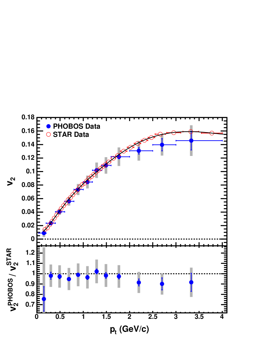
Figure 5: (color online). $v_{2}$ vs. $p_{t}$ for charged hadrons from 0–50% centrality collisions in comparison to data from PHOBOS PHOBOSQM04 . The line is a polynomial fit to the STAR data. The gray error boxes represent the PHOBOS systematic errors. The bottom panel shows the ratio of the PHOBOS data to the polynomial fit.

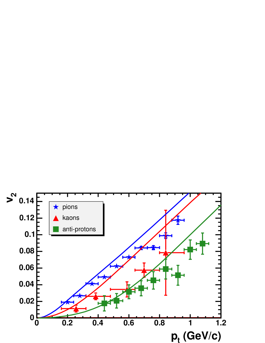
Figure 6: (color online). $v_{2}\{4\}$ vs. $p_{t}$ for identified particles in the 20–60% centrality range. The solid lines are hydrodynamic calculations pasi01 .

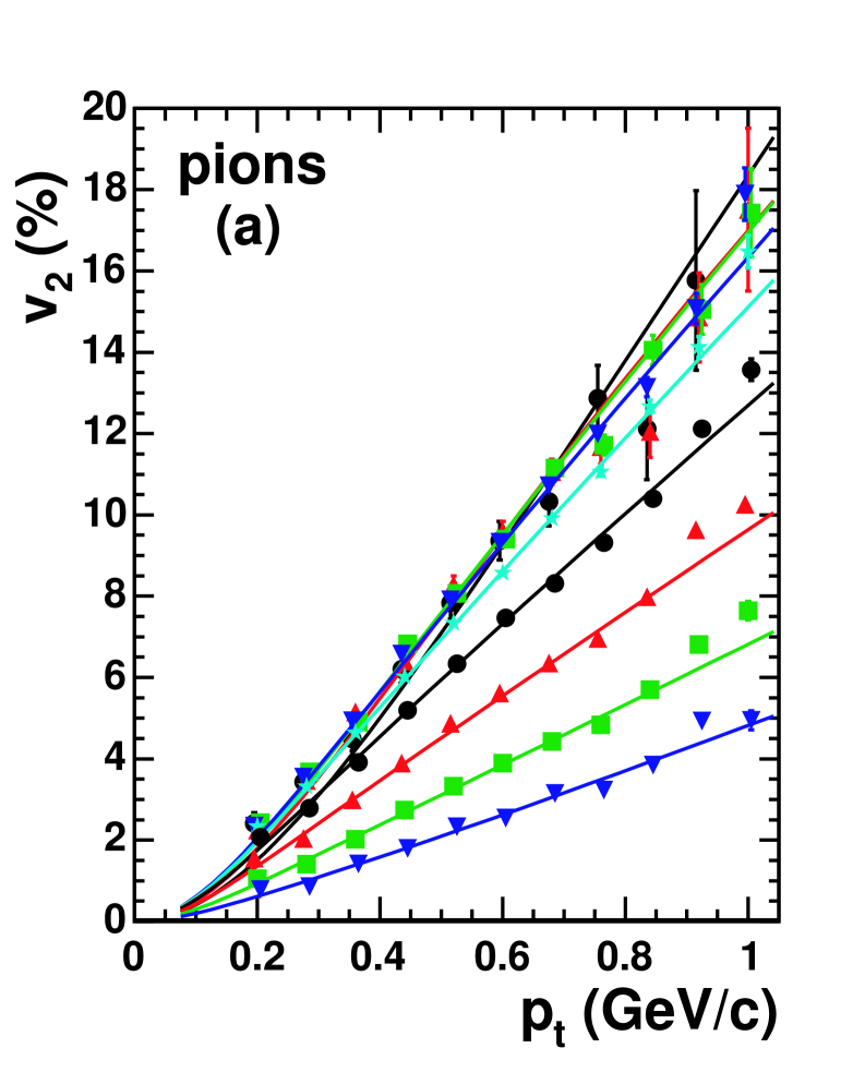
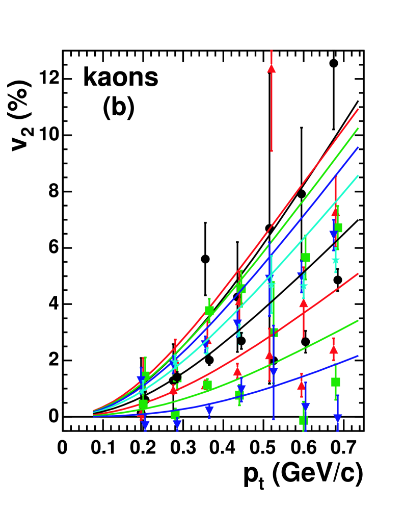
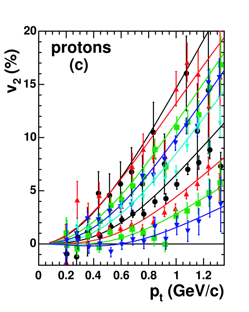
Figure 7: (color online). $v_{2}\{2\}$ vs. $p_{t}$ for charged pions, charged kaons, and anti-protons for the centrality bins (bottom to top) 5 to 10% and in steps of 10% starting at 10, 20, 30, 40, 50, 60, and 70 up to 80%. The solid lines are Blast Wave fits.

Although all the data presented in this paper were collected using the full magnetic field (0.5 $T$) of the STAR detector, some data were also collected using half the magnetic field. Below 0.5 $\mathrm{GeV}/c$ the half field $v_{2}$ values are lower, especially for the more central collisions. These are regions where the $v_{2}$ values are small. Adding the absolute value of 0.0025 to the half field $v_{2}(p_{t})$ data brought the two sets of data into approximate agreement in this $p_{t}$ range. This additive value is for both sets of data analyzed with a dca cut of 2 cm as is done in this paper. The discrepancy gets worse as the upper dca cut decreases. The effect is not understood and none of the half field data are included in this paper. However, a possible explanation is that the half field data have poorer two-track resolution and are more sensitive to track merging, giving a negative nonflow contribution. If true, there could be a possible small residual systematic effect on the full field data. However, the $v_{2}$ results are compared to PHOBOS data PHOBOSQM04 for 0–50% centrality and $0\mbox{$\ <\ $}\eta\mbox{$\ <\ $}1.5$ in Fig. 5. The STAR data is for the TPC integrated also for 0–50% centrality. The full field data presented here agree well with the PHOBOS data.

Results from four-particle cumulants, $v_{2}\{4\}$, are shown in Fig. 6 for particles identified by energy loss in the TPC. Also shown are hydrodynamic calculations pasi01 . The two-particle values, $v_{2}\{2\}$, for pions, kaons, and anti-protons are shown for the individual centralities with Blast Wave fits in Fig. 7. We use only anti-protons at low $p_{t}$ due to contamination of the proton sample from hadronic interactions in the detector material.

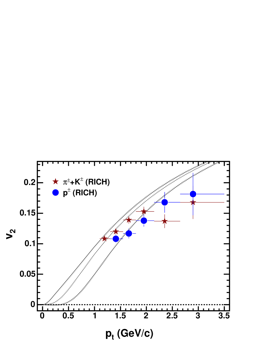
Figure 8: (color online). $v_{2}$ vs. $p_{t}$ for particles identified in the RICH detector from minimum bias collisions. The lines are hydrodynamic calculations pasi01 for pions (upper line), kaons (middle line), and protons (lower line).

Figure 8 shows $v_{2}(p_{t})$ for charged mesons and protons + anti-protons identified in the RICH detector. The experimental results are compared to hydrodynamic calculations pasi01 . In the hydrodynamic picture, the mass ordering of $v_{2}$ (the lighter particles have larger $v_{2}$ than the heavier particles) is predicted to hold at all transverse momenta. Up to $p_{t}\sim 2\$ $\mathrm{GeV}/c$, $v_{2}$ of charged mesons is found to be larger than that of the heavier baryons, in agreement with hydrodynamic predictions. Above $p_{t}=2$ $\mathrm{GeV}/c$, the data seem to indicate a reversed trend where the protons + anti-protons might have larger $v_{2}$ values than the charged mesons.

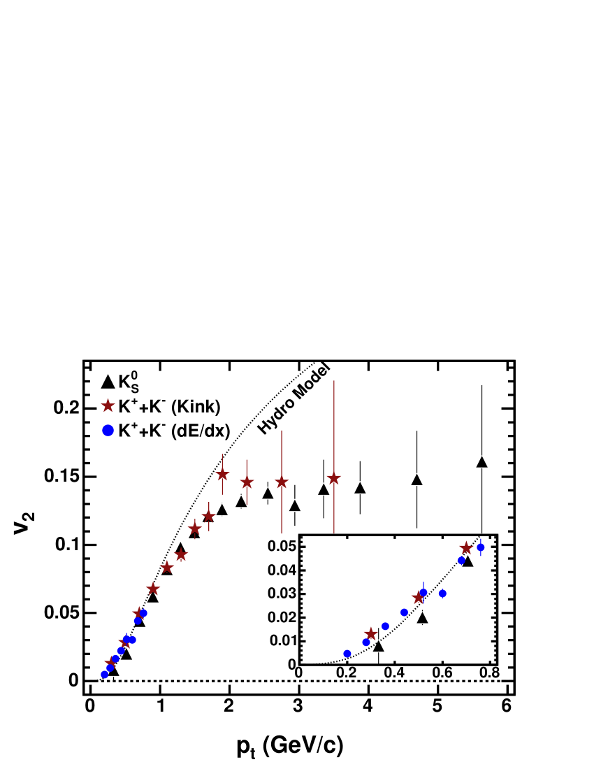
Figure 9: (color online). $v_{2}$ vs. $p_{t}$ for neutral and charged kaons for minimum bias collisions. The $\mathrm{K}^{0}_{S}$ values are from Ref. STAR_Rcp . The hydrodynamic model line is from Ref. pasi01 . The insert expands the low $p_{t}$ region to make the kaons from $dE/dx$ more visible.

Figure 10: (color online). $v_{2}$ vs. $p_{t}$ for strange particles from minimum bias collisions. The STAR $\mathrm{K}^{0}_{S}$ and $\Lambda+\overline{\Lambda}$ values are from Ref. STAR_Rcp . The PHENIX data are from Ref. PHENIXPID . The hydro calculations are from Ref. pasi03 .

From the kink analysis the results are shown in Fig. 9. There were about 0.4 accepted candidate kaons reconstructed per event.

Results are shown in Fig. 10 comparing STAR data for $\mathrm{K}^{0}_{S}$  and $\Lambda+\overline{\Lambda}$  out to 6 $\mathrm{GeV}/c$ with some PHENIX data PHENIXPID , and with hydro calculations pasi03 . For kaons, we can now compare $v_{2}(p_{t})$ for neutral kaons, charged kaons from kinks, and charged kaons from energy loss identification. This is shown in Fig. 9, where the agreement is good, but in the insert one can see that the neutral kaons tend to be slightly lower than the charged kaons.

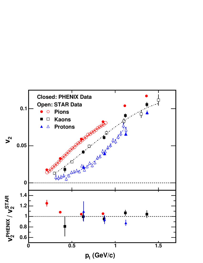
Figure 11: (color online). $v_{2}$ vs. $p_{t}$ for charged pions, charged kaons, and anti-protons from minimum bias collisions in comparison to similar data from PHENIX. The lines are polynomial fits to the STAR data. The bottom panel shows the ratio of the PHENIX data to the polynomial fits.

We can also compare our results in more detail at lower $p_{t}$ with those from PHENIX PHENIXPID . Figure 11 shows $v_{2}(p_{t})$ for charged pions and anti-protons from the energy loss analysis requiring 90% purity, and kaons from the kink analysis. The PHENIX results are for $|\eta|\mbox{$\ <\ $}0.35$, for 0–70% centrality, and for protons and anti-protons combined. In the $p_{t}$ range where the data overlap, the agreement is seen to be good.

It is interesting to see how azimuthal correlations evolve from elementary collisions (p+p) through collisions involving cold nuclear matter (d+Au), and then on to hot, heavy-ion collisions (Au+Au). A convenient quantity for such comparisons is the scalar product. In the case of only “nonflow”, the scalar product should be the same for all three collision systems regardless of their system size. This assumes independent collisions and that other effects like short range correlations are small. Thus, deviations of the scalar product from elementary p+p collisions result from collective motion and/or effects of medium modification.

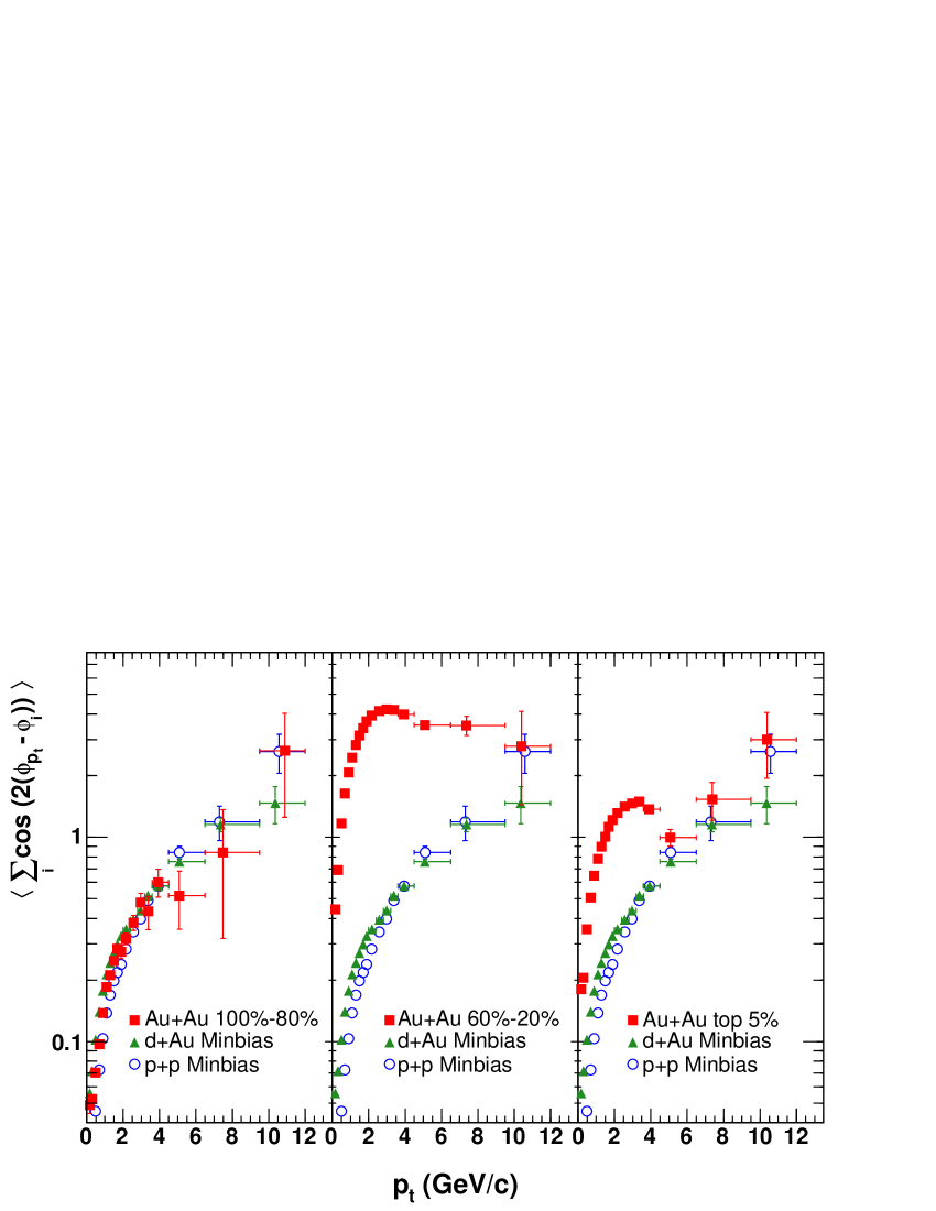
Figure 12: (color online). Charged hadron azimuthal correlations vs. $p_{t}$ in Au+Au collisions (squares) as a function of centrality (peripheral to central from left to right) compared to minimum bias azimuthal correlations in p+p collisions (circles) and d+Au collisions (triangles). The Au+Au and p+p data are from Ref. STARhighPtV2Corr .

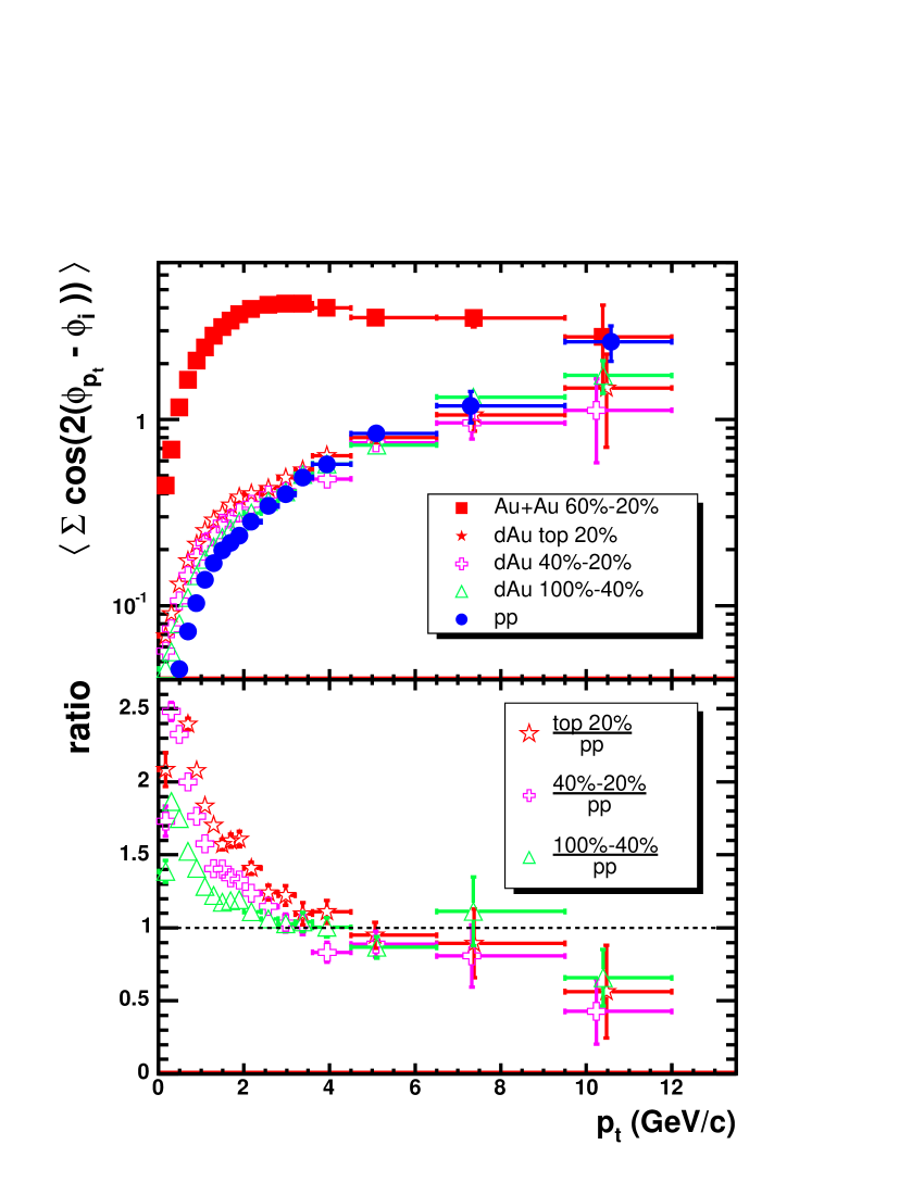
Figure 13: (color online). The top panel shows the charged hadron scalar product vs. $p_{t}$ for different centrality classes in d+Au collisions, and minimum bias p+p collisions. The Au+Au result is put there for a reference. The bottom panel shows the ratio of scalar product from d+Au collisions to minimum bias p+p collisions for three different centrality classes.

Figure 12 shows the scalar product as defined in Eq. 6 as a function of $p_{t}$ for three different centrality ranges in Au+Au collisions compared to minimum bias p+p collisions STARhighPtV2Corr and d+Au collisions. For Au+Au collisions, in middle central events we observe a big deviation from p+p collisions that is due to the presence of elliptic flow, while in peripheral events, collisions are essentially like elementary p+p collisions. The azimuthal anisotropy goes up to 10 $\mathrm{GeV}/c$  but we cannot distinguish whether it is from hydro-like flow or from jet quenching. For $p_{t}$ beyond 5 $\mathrm{GeV}/c$ in central collisions, we again find a similarity between Au+Au collisions and p+p collisions, indicating the dominance of nonflow effects. The scalar product in d+Au collisions is relatively close to that from p+p collisions but there is a finite difference at low $p_{t}$. This difference is small if compared to the difference between middle central Au+Au collisions and minimum bias p+p collisions. If we examine the difference by looking in d+Au collisions at different event classes that are defined by the multiplicity from the Au side (Fig. 13), we find that the scalar product in d+Au increases as a function of multiplicity class, which is contradictory to Au+Au collisions, in which the differences rise and fall as a function of centrality; a typical pattern that is caused by collective flow. The trend in d+Au could be explained by the Cronin effect, because in high multiplicity events, the Cronin effect is expected to produce more collective motion among soft particles in order to generate a high $p_{t}$ particle dAu . To further test the Cronin effect hypothesis, we studied the asymmetry of the scalar product in d+Au collisions in Fig. 14. The ratio of scalar product from the Au side divided by that from the deuteron side is greater than one at low $p_{t}$, and decreases to $\sim$0.9 above $2~{}\mbox{$\mathrm{GeV}/c$}$. This indicates that there is more collective motion for $p_{t}\mbox{$\ >\ $}2~{}\mbox{$\mathrm{GeV}/c$}$ in the deuteron side and $p_{t}\mbox{$\ <\ $}1~{}\mbox{$\mathrm{GeV}/c$}$ in the Au side, which is again consistent with the Cronin effect. Recently, the Cronin effect has been explained by final-state recombination Hwa2004 . However the influence of recombination on azimuthal correlations needs detailed study. In addition to spectra, the scalar product results open new possibilities for testing these models.

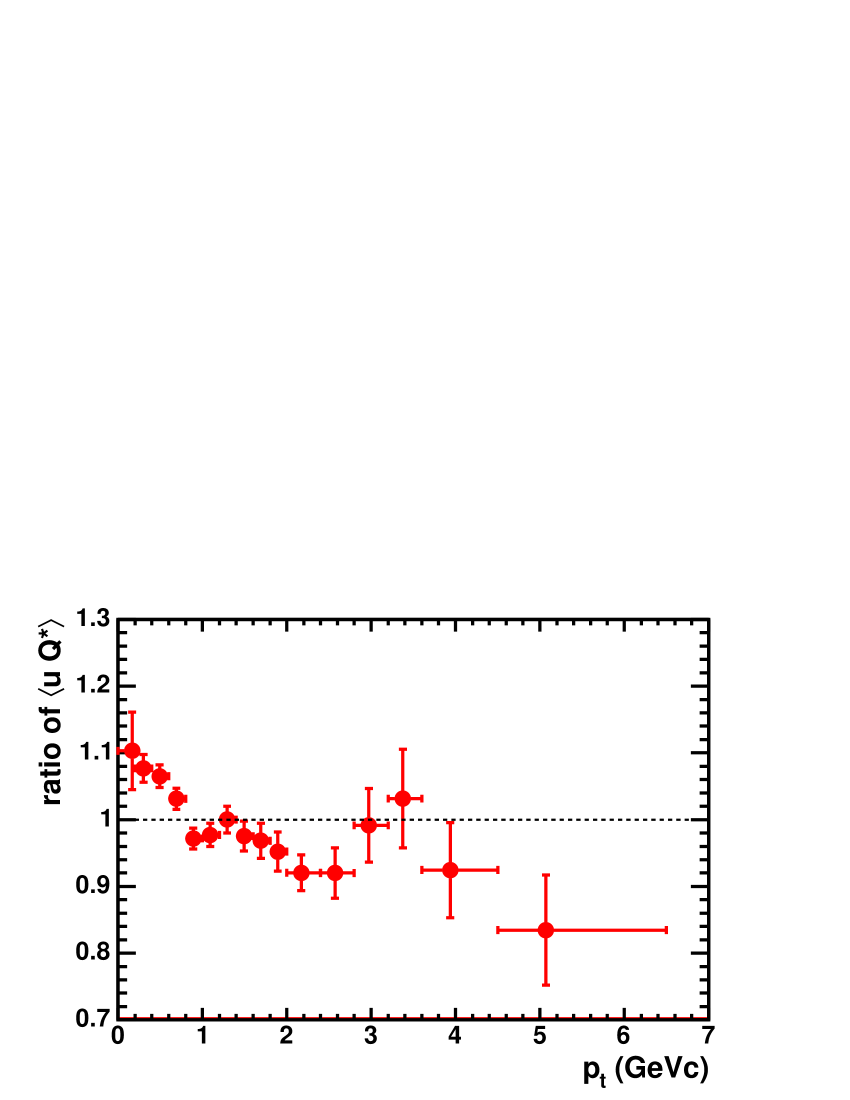
Figure 14: (color online). The ratio of the scalar product from Au side ($-1.0\mbox{$\ <\ $}\eta\mbox{$\ <\ $}$$-0.5$) to that from deuteron side ($0.5\mbox{$\ <\ $}\eta\mbox{$\ <\ $}1.0$) vs. $p_{t}$ from minimum bias collisions.

IV.2.2 The forward regions

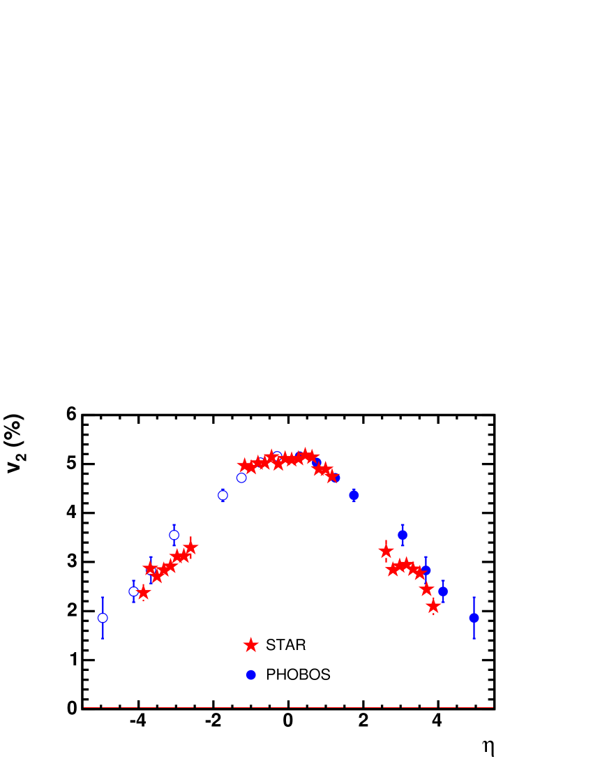
Figure 15: (color online). Charged hadron $v_{2}$ vs. $\eta$ at $\mbox{$\sqrt{s_{\mathrm{NN}}}$}=200$ GeV for STAR minimum bias (stars) and PHOBOS PHOBOSQM04 mid-central (15–25%) centrality (circles). The open circles are PHOBOS data reflected about mid-rapidity.

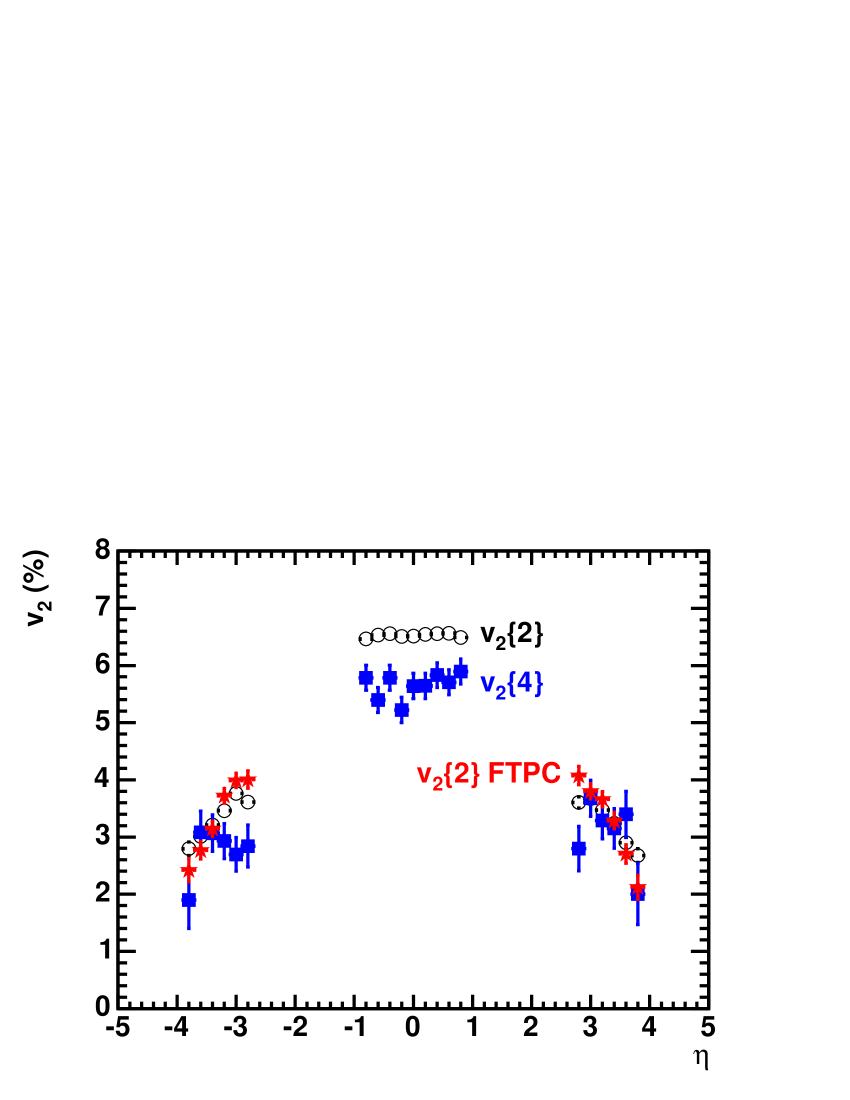
Figure 16: (color online). Charged hadron $v_{2}$ vs. $\eta$ for 20–70% centrality collisions including the FTPC regions. The open circles are $v_{2}\{2\}$, the filled squares are $v_{2}\{4\}$ and the stars are $v_{2}\{2\}$ for only FTPC particles, not using the main TPC particles.

Our measurements of elliptic flow $v_{2}(\eta)$ for charged hadrons at forward pseudorapidities along with those from the central region are shown in Fig. 15. The published results PHOBOS ; PHOBOSQM04 obtained by the PHOBOS collaboration showing a bell-shaped curve are confirmed. We observe a fall-off by a factor of 1.8 comparing $v_{2}(\eta=0)$ with $v_{2}(\eta=3)$. While STAR determined the event plane near mid-rapidity, PHOBOS did it at forward rapidities, which probably accounts for the slightly less fall-off that they see. Both measurements were done using the standard method. Figure 16 compares our results for $v_{2}$ obtained with the method of two-particle cumulants, $v_{2}\{2\}$, to that for four-particle cumulants, $v_{2}\{4\}$. The difference at mid-rapidity will be discussed in Sec. V. The FTPC $v_{2}\{4\}$ values are not quite symmetric about mid-rapidity, but not unreasonable considering the statistical errors. Within the errors in the FTPC regions, the values from the different methods are about the same.

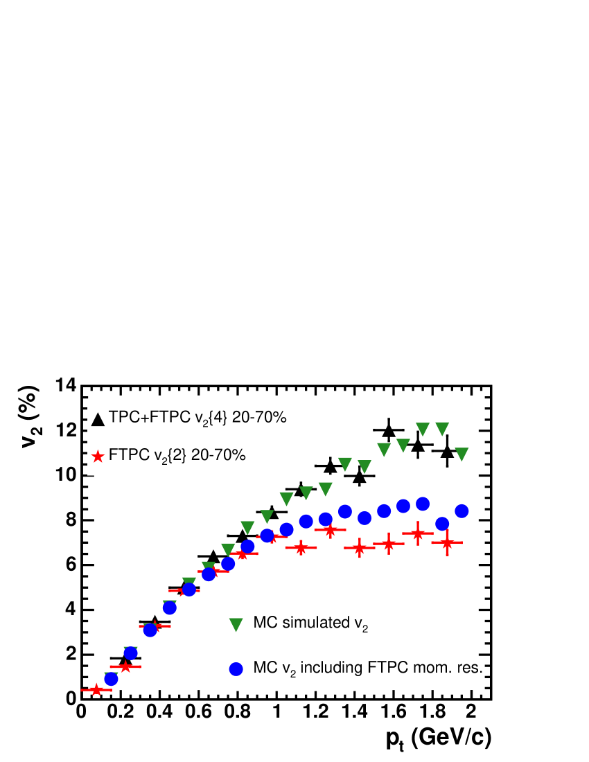
Figure 17: (color online). Charged hadron $v_{2}\{2\}$ vs. $p_{t}$ for centrality 20–70% in the FTPC ($2.5\mbox{$\ <\ $}|\eta|\mbox{$\ <\ $}4.0$) regions (stars) compared to $v_{2}\{4\}$ in the TPC + FTPCs (up-triangles). The down-triangles are Monte Carlo results fit to the up-triangles, and the solid circles include the FTPC momentum resolution.

Figure 17 shows $v_{2}\{4\}(p_{t})$ obtained from the four-particle cumulant method. Since there are many more particles in the main TPC than in the FTPCs, these $v_{2}$ values are mainly at mid-rapidity. $v_{2}\{4\}$, which is much less sensitive to nonflow effects, is compared to $v_{2}\{2\}$ at forward rapidities, where nonflow may be small. The observed flattening at $p_{t}$ values around 1 $\mathrm{GeV}/c$ for the FTPC measurements might be explained by the momentum resolution of the FTPCs. To quantify the influence of the momentum resolution a Monte-Carlo simulation of $v_{2}(p_{t})$ based on the measurements at mid-rapidity was done, but the input $\eta$ and $p_{t}$ spectra were obtained from measurements of the Au+Au minimum bias data at forward rapidities. Results of embedding charged pions (neglecting protons) in real Au+Au events up to 5% of the total multiplicity in the FTPCs were used to estimate the momentum resolution as a function of $\eta$ and $p_{t}$. At $\eta=3.0$ the momentum resolution goes from 10% at low $p_{t}$ to 35% at $p_{t}=2.0\ \mbox{$\mathrm{GeV}/c$}$, but gets about a factor of two worse at $\eta=3.5$. In Fig. 17 the MC simulation $v_{2}(p_{t})$ including the momentum resolution of the FTPCs seems to explain the observed flattening by smearing low $p_{t}$ particles to higher $p_{t}$. Thus we can not conclude that the shape of the $p_{t}$ dependence of elliptic flow at forward rapidities is different from that at mid-rapidity, even though the values integrated over $p_{t}$ are considerably smaller as shown in Fig. 16.

IV.2.3 High $p_{t}$

Hadron yields at sufficiently high transverse momentum in Au+Au collisions are believed to contain a significant fraction originating from the fragmentation of high energy partons resulting from initial hard scatterings. Calculations based on perturbative QCD predict that high energy partons traversing nuclear matter lose energy through induced gluon radiation quenching . Energy loss (jet quenching) is expected to depend strongly on the color charge density of the created system and the traversed path length of the propagating parton. Consistent with jet quenching calculations, strong suppression of the inclusive high-$p_{t}$ hadron production centrality ; highptsuppression and back-to-back high-$p_{t}$ jet-like correlation btob compared to the reference p+p and d+Au systems was measured in central Au+Au collisions at RHIC. In non-central heavy-ion collisions, the geometrical overlap region has an almond shape in the transverse plane, with its short axis lying in the reaction plane. Partons traversing such a system, on average, experience different path-lengths and therefore different energy loss as a function of their azimuthal angle with respect to the reaction plane. This leads to an azimuthal anisotropy in particle production at high transverse momenta. Finite values of $v_{2}$ were measured in non-central Au+Au collisions for $p_{t}$ up to $\sim$ 7–8 $\mathrm{GeV}/c$ STARchargedhighpt ; STARhighPtV2Corr using the standard reaction plane method and two- and four-particle cumulants. The measurements of azimuthal anisotropies at high transverse momenta with the standard reaction plane method and two-particle cumulants are influenced by the contribution from the inter- and intra-jet correlations. These correlations, in general, may not be related to the true reaction plane orientation and, hence, are a source of nonflow effects. A multi-particle cumulant analysis, which has been shown to suppress nonflow effects, may give lower $v_{2}$ values because of the opposite sensitivity of $v_{2}\{2\}$ and $v_{2}\{4\}$ to the fluctuations of $v_{2}$ itself described in Sec. V.2 and Ref. epsilonMC .

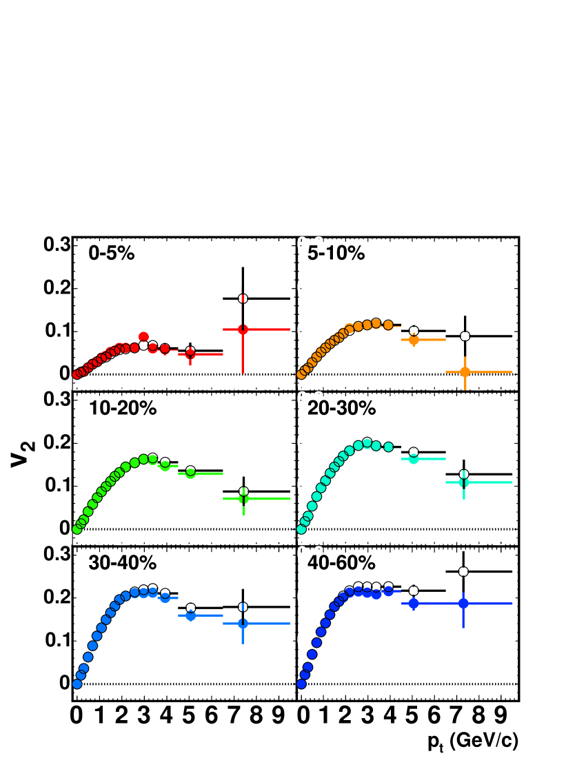
Figure 18: (color online). $v_{2}$ vs. $p_{t}$ for charged hadrons for different centrality bins. The standard reaction plane method is shown by open symbols and the modified reaction plane method by solid symbols.

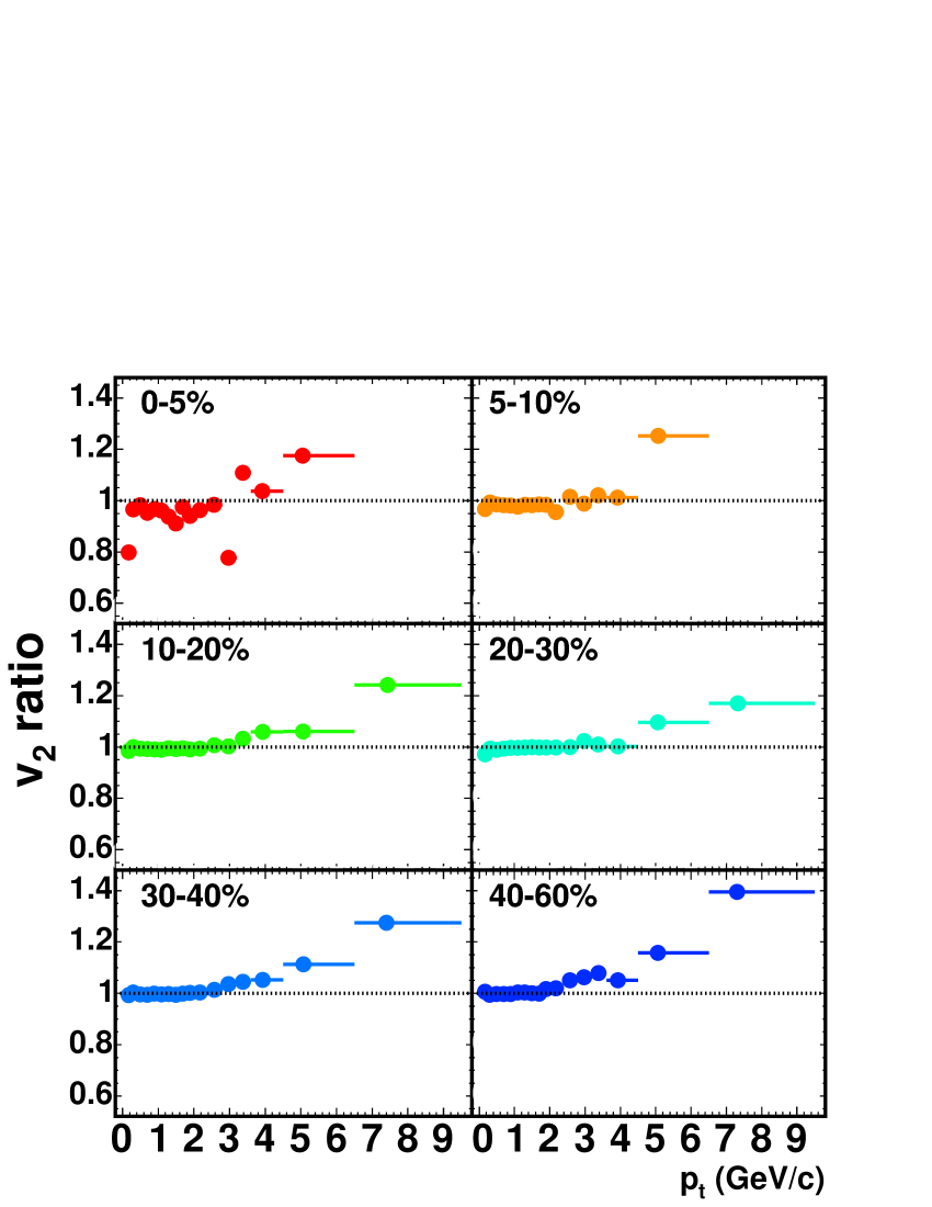
Figure 19: (color online). $v_{2}$ for the standard reaction plane method divided by $v_{2}$ for the modified reaction plane method vs. $p_{t}$ for charged hadrons in different centrality bins. Error bars are not shown as the same dataset is used for both methods.

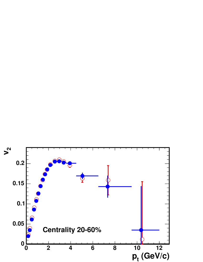
Figure 20: (color online). $v_{2}$ vs. $p_{t}$ for charged hadrons from the modified reaction plane method (solid circles). Open circles (from Ref. STARhighPtV2Corr , Fig. 2) are the two-particle cumulant results after subtracting the correlations measured in p+p collisions. Error bars show statistical uncertainties only.

Figure 18 shows the differential elliptic flow $v_{2}$ obtained with the standard and modified reaction plane methods as a function of $p_{t}$ for different collision centralities. The modified event plane method excludes particles within $|\Delta\eta|\mbox{$\ <\ $}$ 0.5 around the highest $p_{t}$ particle. For both methods $v_{2}$ rises linearly up to $p_{t}=1$ $\mathrm{GeV}/c$, then deviates from a linear rise and saturates for $p_{t}\mbox{$\ >\ $}$3 $\mathrm{GeV}/c$ for all centralities. Fig. 9 shows a similar behavior. Although the statistical errors are large, we observe a systematic difference in Fig. 18 for the $v_{2}$ values obtained with the two methods at high transverse momenta. This is better illustrated in Fig. 19, where we show the ratio of $v_{2}$ obtained with the standard and modified reaction plane methods. At low transverse momenta ($p_{t}\mbox{$\ <\ $}$ 2 $\mathrm{GeV}/c$), the $v_{2}$ values are very similar for both methods. At higher transverse momenta, $v_{2}$ is systematically larger for the standard reaction plane method. For more peripheral collisions this effect is larger, and it also begins at lower $p_{t}$. The modified reaction plane method seems to eliminate at least some of the nonflow effects at high transverse momenta (up to 15–20% at $p_{t}=$ 5–6 $\mathrm{GeV}/c$ in the most peripheral collisions). The contribution of the azimuthal correlations not related to the reaction plane orientation has been previously studied using p+p collisions STARhighPtV2Corr . In p+p collisions, all correlations are considered to be of nonflow origin. In Fig. 12 the azimuthal correlations in mid-central Au+Au collisions are very different from those in p+p collisions in both magnitude and $p_{t}$ dependence. Figure 20 shows the modified reaction plane results on $v_{2}(p_{t})$ for charged hadrons of centrality 20–60%. We find a very good agreement of $v_{2}$ from the modified reaction plane analysis with the two-particle cumulant results after subtracting the correlations measured in p+p collisions STARhighPtV2Corr . Neither of these modified methods which seem to be necessary at high $p_{t}$ give results which differ from the simple standard method below $p_{t}$ of 2 $\mathrm{GeV}/c$, and thus are not used in the other analyses of this paper.

IV.3 Higher harmonics

IV.3.1 The central region

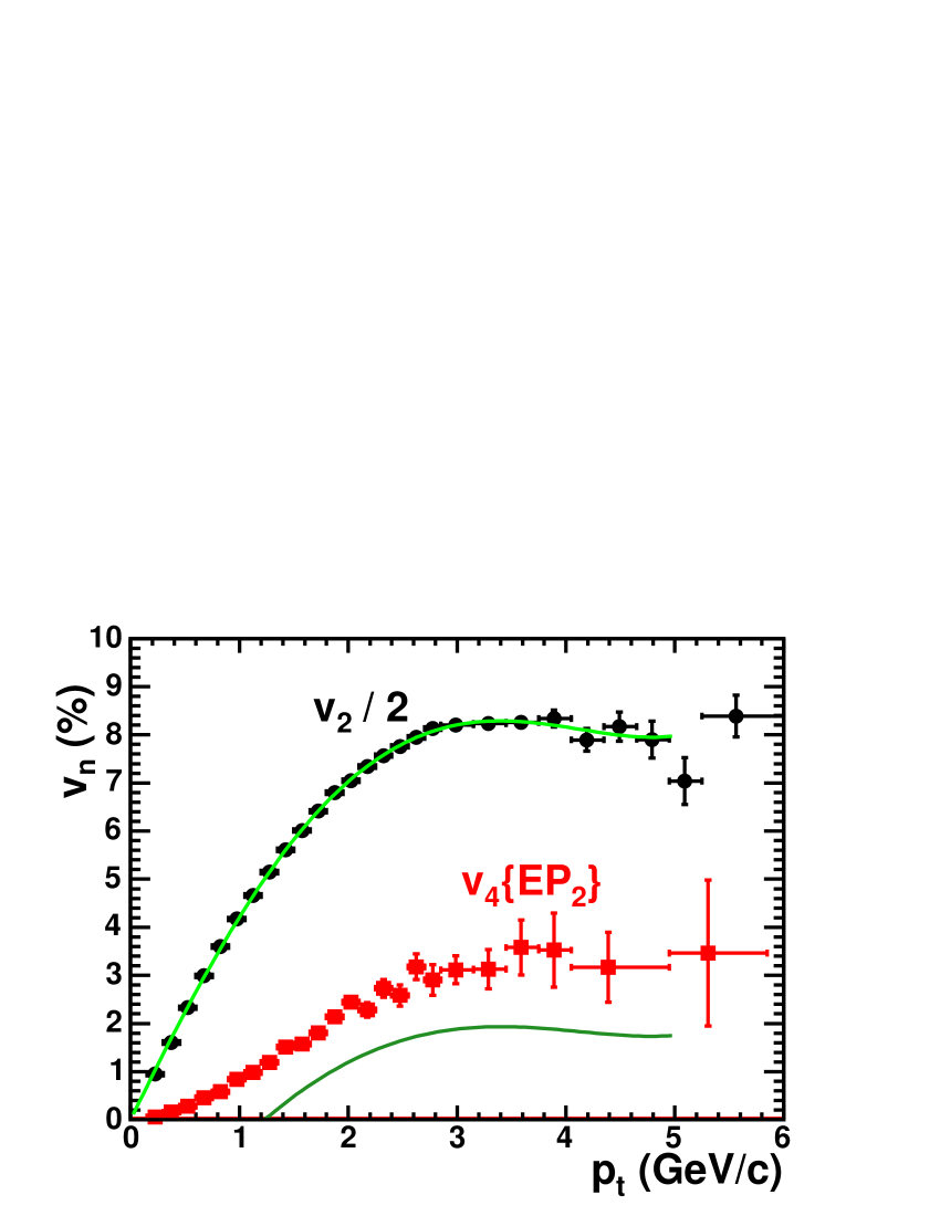
Figure 21: (color online). $v_{2}$ scaled down by a factor of 2, and $v_{4}\{\mathrm{EP}_{2}\}$ vs. $p_{t}$ for charged hadrons from minimum bias events. Using a fit to the $v_{2}$ values, the lower solid line is the predicted $v_{4}$ needed to just remove the “peanut” waist (see text).

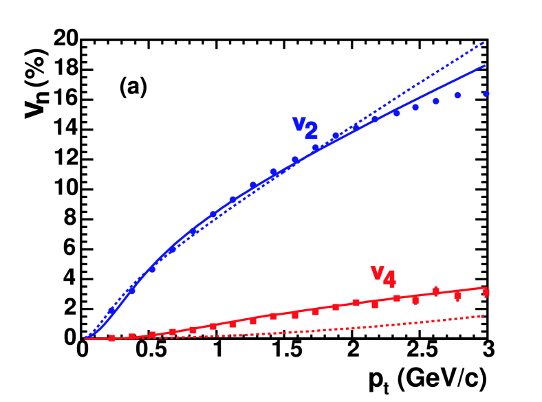
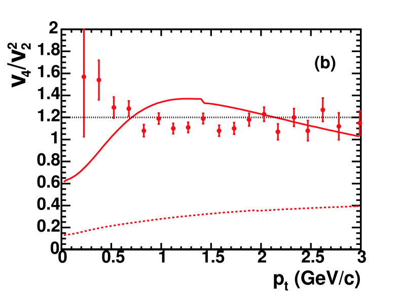
Figure 22: (color online). Graphs of $v_{n}$ and $v_{4}/v_{2}^{2}$. The dashed lines are surface shell Blast Wave fits with no $\rho_{4}$ or $s_{4}$ terms (See Sec. VI.4) to the charged hadron $v_{2}$ minimum bias data. The resultant ratio $v_{4}/v_{2}^{2}$ is shown as the lower dashed line in the ratio graph (b). The solid lines are the fits with the addition of $\rho_{4}$ and $s_{4}$. The resultant ratio $v_{4}/v_{2}^{2}$ is shown as the solid curve in the ratio graph (b). The dotted line in the ratio graph (b) at 1.2 represents the average value of the data.

Our results for charged hadron $v_{4}$ and $v_{6}$ from this study have already been published STARv1v4 ; STARv4 , and $v_{4}(p_{t})$ is shown again in Fig. 21. It also was found that $v_{4}$ scales as $v_{2}^{2}$. The value of $v_{4}/v_{2}^{2}$ was found to be 1.2, almost independent of $p_{t}$ STARv4 , as can be seen in the ratio graph of Fig. 22 (b).

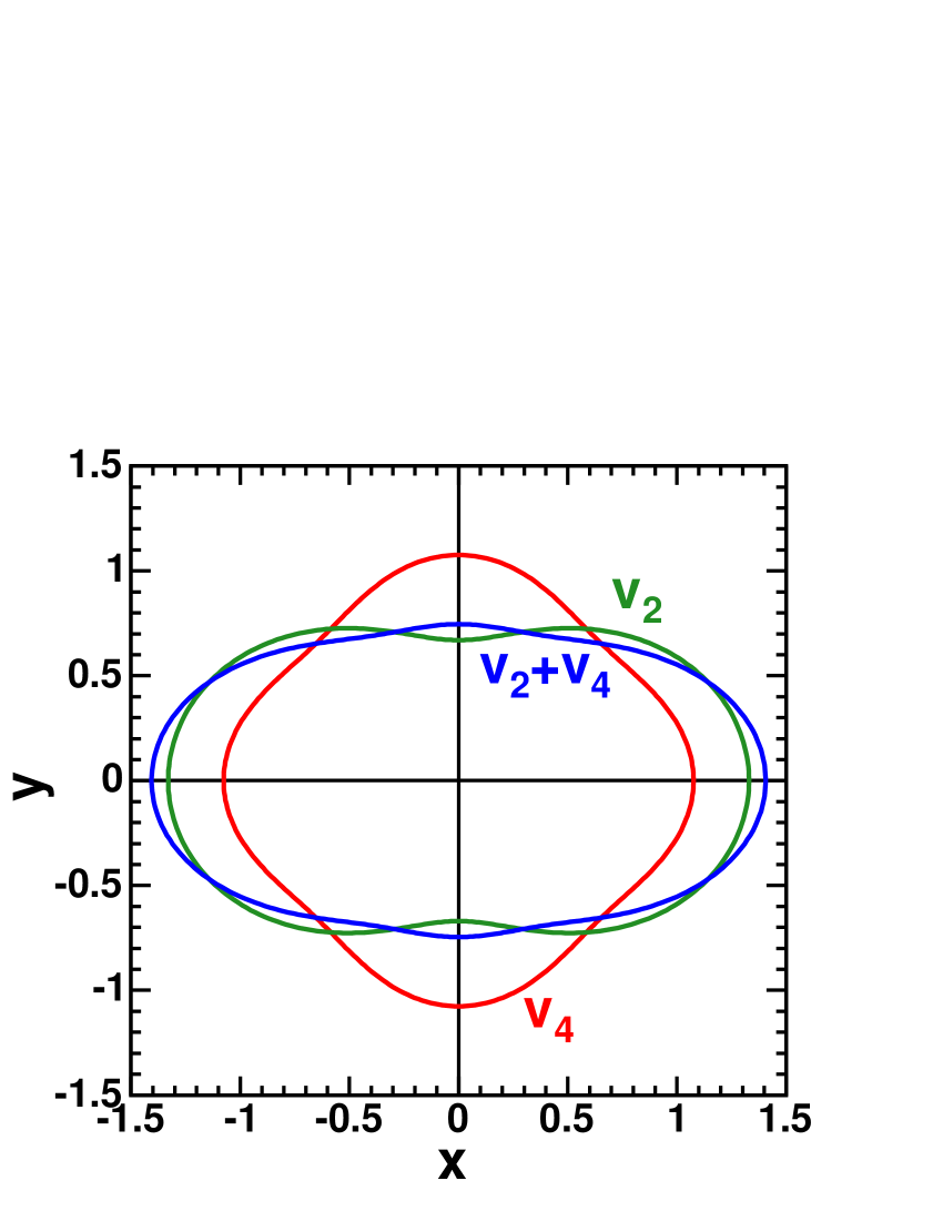
Figure 23: (color online). A polar graph of the distribution $1+2v_{2}\cos(2\phi)+2v_{4}\cos(4\phi)$ where $\phi$ is the azimuthal angle relative to the positive $x$ axis. Plotted are the distributions for $v_{2}=16.5$% showing the waist, $v_{4}=3.8$% having a diamond shape, and both coefficients together.

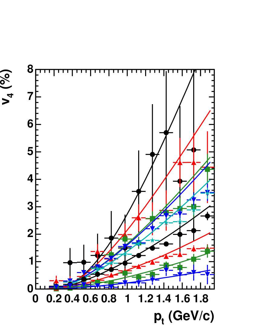
Figure 24: (color online). $v_{4}\{\mathrm{EP}_{2}\}$ vs. $p_{t}$ for charged hadrons for the centrality bins (bottom to top) 5 to 10% and in steps of 10% starting at 10, 20, 30, 40, 50, 60, and 70 up to 80%. The solid lines are Blast Wave fits.

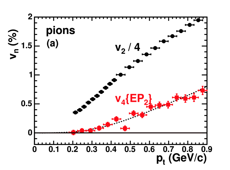
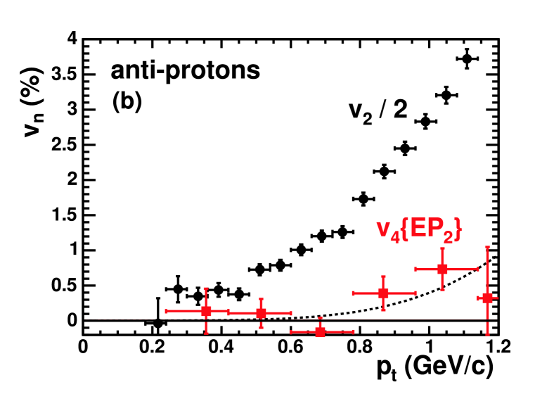
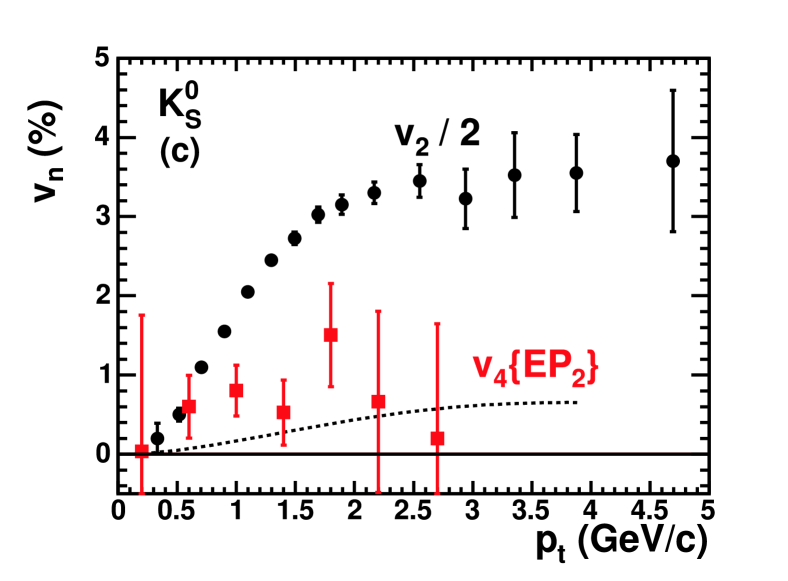
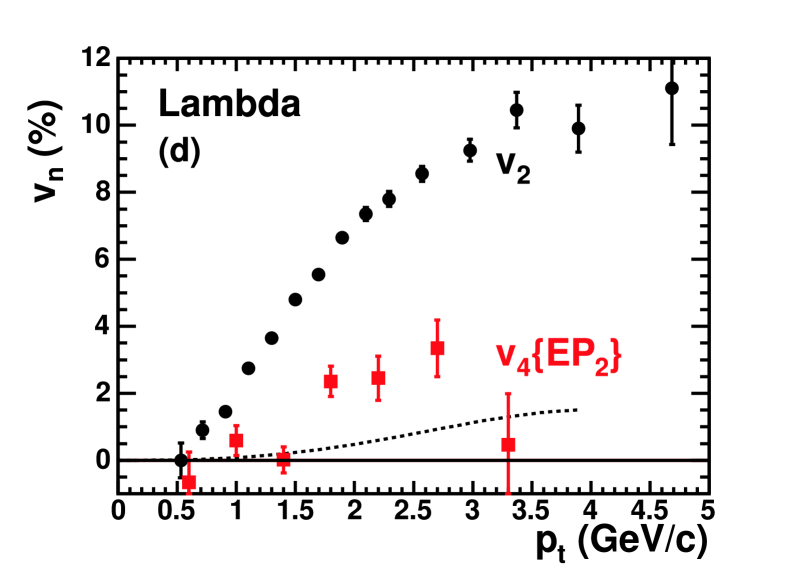
Figure 25: (color online). $v_{4}\{\mathrm{EP}_{2}\}$ and $v_{2}$ vs. $p_{t}$ for identified pions, anti-protons, $\mathrm{K}^{0}_{S}$ , and $\Lambda+\overline{\Lambda}$ for minimum bias collisions. The dashed lines are at $1.2~{}v_{2}^{2}$.

Kolb Kolb_v4 pointed out that for large $v_{2}$ the azimuthal shape in momentum space described by the $v_{n}$ Fourier expansion is no longer elliptic, but becomes “peanut” shaped. Using our high $p_{t}$ plateau experimental values, we show this in Fig. 23. Kolb also gives an equation for the amount of $v_{4}$ needed to just eliminate the peanut waist. Figure 21 shows that the experimental $v_{4}$ values considerably exceed this value.

Fig. 24 shows the $\mbox{$v_{4}\{\mathrm{EP}_{2}\}$}(p_{t})$ values for the individual centralities with filled elliptic cylinder Blast Wave fits assuming all charged hadrons have the mass of a pion.

Using the probability PID method STARPID ; TangThesis for charged pions and anti-protons, and a topological analysis method for $\mathrm{K}^{0}_{S}$ and $\Lambda+\overline{\Lambda}$ , we obtain the $\mbox{$v_{4}\{\mathrm{EP}_{2}\}$}(p_{t})$ and $v_{2}(p_{t})$ values shown in Fig. 25. For pions the $v_{2}^{2}$ scaling ratio is shown in Fig. 26. To make this graph it was necessary to combine data points to get reasonable errors bars for the ratio because the $v_{4}$ values are so small. The resulting scaling ratio is consistent with that for charged hadrons shown in the Fig. 22 (b) ratio graph.

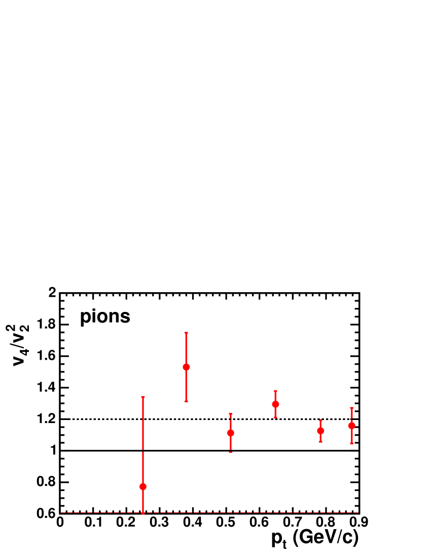
Figure 26: (color online). The ratio $v_{4}/v_{2}^{2}$ vs. $p_{t}$ for identified pions. The dashed line is at $v_{4}/v_{2}^{2}=1.2$.

IV.3.2 The forward regions

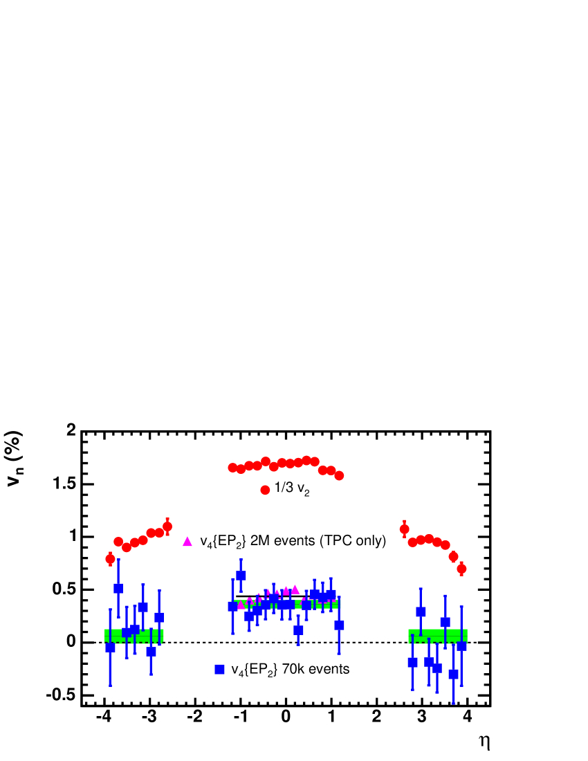
Figure 27: (color online). Comparison of $v_{2}$ to $v_{4}\{\mathrm{EP}_{2}\}$ for charged hadrons from minimum bias collisions as a function of pseudorapidity. The fourth harmonic (squares) is consistent with zero at forward pseudorapidities but not at mid-rapidity. $v_{2}$ is shown by circles, scaled by a factor of 1/3 to fit on the plot. The larger dataset available for the TPC only (triangles) confirms our measurement of $v_{4}\{\mathrm{EP}_{2}\}$ at mid-rapidities.

In Fig. 27 the fourth harmonic $v_{4}\{\mathrm{EP}_{2}\}$ shows an average value of $(0.4\pm 0.1)\%$ in the pseudorapidity coverage of the TPC ($|\eta|\mbox{$\ <\ $}1.2$). In contrast, its value of $(0.06\pm 0.07)\%$ in the forward regions is consistent with zero, with a $2\sigma$ upper limit of 0.2%. Therefore the relative fall-off of $v_{4}$ from $\eta=0$ to $\eta=3$ appears to be stronger than for $v_{2}$. This behavior is consistent with $v_{4}\ \propto\ v_{2}^{2}$ scaling.

IV.3.3 High $p_{t}$

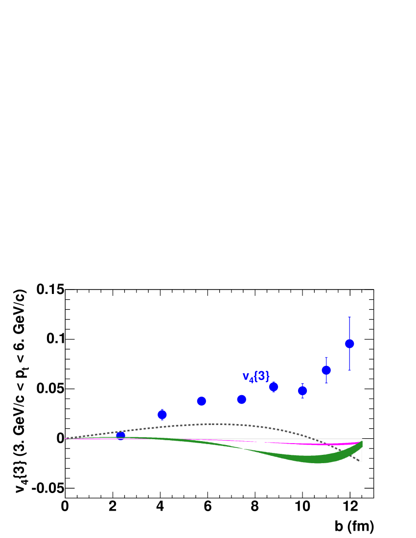
Figure 28: (color online). High $p_{t}$ charged hadron $v_{4}\{3\}$ integrated for $3\leq p_{t}\leq 6\ \mbox{$\mathrm{GeV}/c$}$ vs. impact parameter $b$, compared to models of particle absorption: dashed curve is the hard shell, higher narrow band is Woods-Saxon, lower wider band is hard sphere. The bands have widths for absorption to match the observed range of yield suppression.

It has been emphasized that $v_{4}$ has a stronger potential than $v_{2}$ to constrain jet-quenching model calculations Kolb_v4 . Following the same procedure as described in Ref. STARhighPtV2Corr , we plot in Fig. 28 the $v_{4}\{3\}$ from moderately high $p_{t}$. It should be noted that the two most peripheral points go up rather than down as they do for $v_{2}$, in apparent violation of $v_{4}/v_{2}^{2}$ scaling at this high $p_{t}$. We compare the results with the fourth harmonic anisotropy generated by energy loss in a static medium with a Woods-Saxon density profile, hard sphere (step function in density), and the extreme case – hard shell limit. The results are shown in Fig. 28. The dashed curve corresponds to the hard shell; the upper and lower bands corresponds to a parameterization of jet energy loss where the absorption coefficient is set to match the suppression of the inclusive hadron yields. The lower and upper boundaries of the bands around $b=11$ fm correspond to an absorption that gives suppression factors of 5 and 3, respectively. Note that compared to the case of $v_{2}$ STARhighPtV2Corr , the calculations are less sensitive to the suppression factors (narrow bands). These model calculations cannot reproduce the correct sign of $v_{4}$ over the whole range of impact parameters, and neither can they reproduce the magnitude of $v_{4}$. A similar observation was made for the magnitude of $v_{2}$ in this $p_{t}$ range in Ref. STARhighPtV2Corr . In the present case, evidently the absorption of jet particles is not the dominant mechanism for producing $v_{4}$ in this $p_{t}$ range.

V Methods comparisons

In addition to the standard and scalar product methods already described, there are also several subevent methods where each particle is correlated with the event plane of the other subevent. If the subevents are produced randomly, we will call this the random subs method. If the particles are sorted according to their pseudorapidity, we will call it the eta subs method. In these methods, since only half the particles are used for the event plane, the statistical errors are approximately $\sqrt{2}$ larger, but autocorrelations do not have to be removed since the particle of interest is not in the other subevent.

Another method involves fitting the distribution of the lengths of the flow vectors normalized by the square root of the multiplicity Voloshin-Zhang ; OlliQM95 ; STARcumulants :

$$q_{n}=Q_{n}/\sqrt{M}$$ (7)

$$\frac{dP}{q_{n}dq_{n}}=\frac{1}{\sigma_{n}^{2}}e^{\displaystyle{-\frac{v_{n}^{2}M+q_{n}^{2}}{2\sigma_{n}^{2}}}}I_{0}(\frac{q_{n}v_{n}\sqrt{M}}{\sigma_{n}^{2}}),$$ (8)

where $I_{0}$ is the modified Bessel function and

$$\sigma_{n}^{2}=0.5(1+g_{n}).$$ (9)

Nonflow effects are fit with the parameter $g_{n}$. The values of $M$ are in Table 2.

V.1 Comparisons

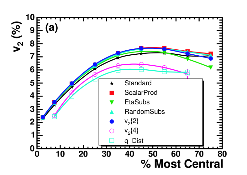
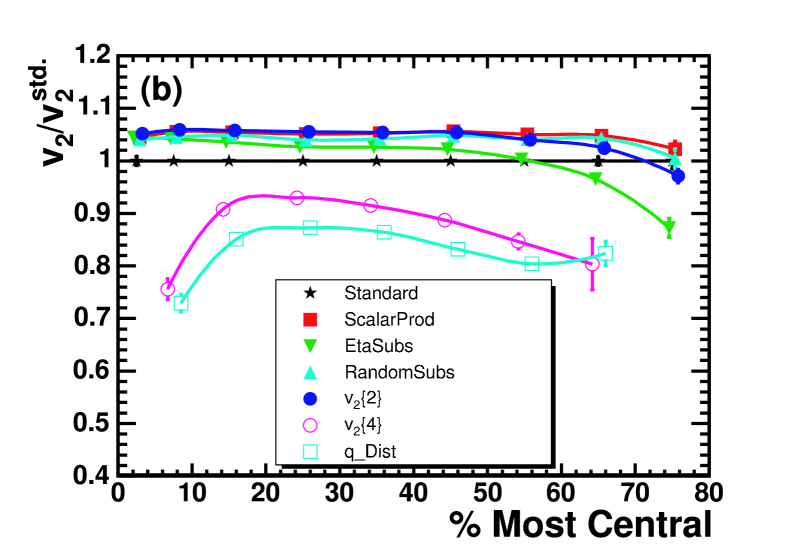
Figure 29: (color online). Charged hadron $v_{2}$ integrated over $p_{t}$ and $\eta$ vs. centrality for the various methods described in the text. In panel (b) is shown the ratio of $v_{2}$ to the standard method $v_{2}$.

To make a precise comparison of the various methods we have calculated $v_{2}$ integrated over $p_{t}$ and $\eta$ for the main TPC, and plotted it vs. centrality in Fig. 29 (a). To make the comparison valid we have used the same events and the same cuts, which are shown in Table 1. The integrated values have not been corrected for the missing regions beyond the integration limits given. The systematic error at the lowest $p_{t}$ values ($\approx$ 0.2 $\mathrm{GeV}/c$) is probably larger than at higher $p_{t}$, but its contribution to the integrated $v_{n}$ values is small because the yield is so low there. For constructing the $Q$ vector, linear $p_{t}$ weighting was used for all methods except the $q$-distribution method, where no weighting was used. From the agreement of different software implementations of the same method, we estimate a relative systematic error (not included) of at least 2% of the $v_{2}$ values shown.

The results fall generally into two bands: those for two-particle correlations methods, and those for multi-particle methods. The difference is due either to the decreased sensitivity of the multi-particle methods to nonflow effects, or to their increased sensitivity to fluctuation effects epsilonMC . Thus, the “true” flow values must be between these two limits. To expand the graph in order to look for small differences we also have plotted the ratios to the standard method in Fig. 29 (b). It appears that the standard method is about 5% lower than the other two-particle correlation methods. We first thought that this might be due to nonflow effects affecting the extrapolation in the standard method from the subevent resolution to the full event resolution. However, it also could be due to the fact that the standard method uses twice as many particles as the subevent methods, and therefore is less sensitive to nonflow effects. But this does not explain why the scalar product method falls in the band with the subevents. The values from the eta subevent method decrease for peripheral collisions. This could be due to decreased nonflow effects for particles separated in pseudorapidity.

V.2 Nonflow effects and fluctuations

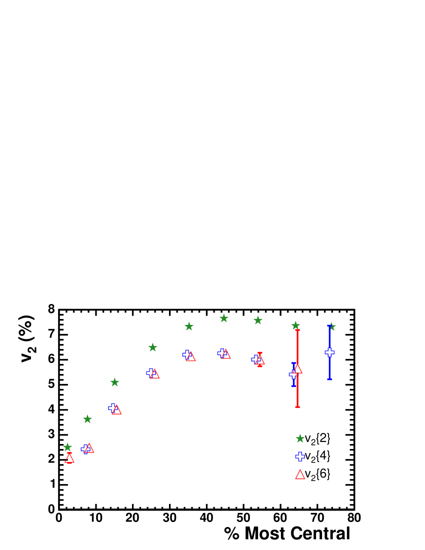
Figure 30: (color online). Charged hadron $v_{2}\{2\}$, $v_{2}\{4\}$, and $v_{2}\{6\}$ integrated values as a function of centrality.

Particle correlations which are not correlated with the reaction plane are called nonflow effects when they affect $v_{n}$. Figure 30 shows the two, four, and six-particle integral cumulant $v_{2}$ values using the cuts in Table 1. The four- and six- particle results agree, showing that nonflow effects are eliminated already with four-particle correlations.

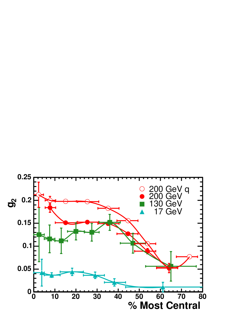
Figure 31: (color online). The nonflow parameter, $g_{2}$, as a function of centrality. The solid points are from the cumulant method. The open circles are from the $q$-distribution method.

Nonflow can be calculated by the difference between the squares of the two-particle and four-particle cumulant $v_{2}$ values, normalized with the number of wounded nucleons from Table 2. Thus, STARcumulants ; NA49 ; v13

$$g_{2}=N_{WN}\cdot(v_{2}^{2}\{2\}-v_{2}^{2}\{4\}),$$ (10)

which is shown in Fig. 31 for $\mbox{$\sqrt{s_{\mathrm{NN}}}$}=$ 200 GeV, 130 GeV, and from the SPS at 17.2 GeV NA49 . The SPS $g_{2}$ values were divided by the multiplicity used and multiplied by $N_{WN}$, both given in that paper NA49 . From the $q$-distribution method of calculating $v_{2}$, $g_{2}$ can be obtained by the increase in the width of the distribution from Eq. (9). (It should be pointed out that in these fits, $v_{2}$ and $g_{2}$ are somewhat anti-correlated.) For the $q$-distribution method the $g_{2}$ values were also divided by the multiplicity used and multiplied by $N_{WN}$. Thus, all four results have been renormalized to use the number of wounded nucleons. Instead of being independent of centrality as originally thought, $g_{2}$ seems to decrease somewhat for the more peripheral collisions, but appears to have the same shape for all the systems. The 17 GeV results may be different from the others because $g_{2}$ could vary with the acceptance of the detector. At 200 GeV it is possible that $g_{2}$ from the $q$-distribution method is larger than from the cumulant method because of real fluctuations in $v_{2}$ broadening the $q$-distribution. Although the definition of $q$ in Eq. (7) removes most of the multiplicity dependence of $Q$, Eq. (8) still contains the quantity $M$, and thus is subject to the spread in $M$ in a centrality bin.

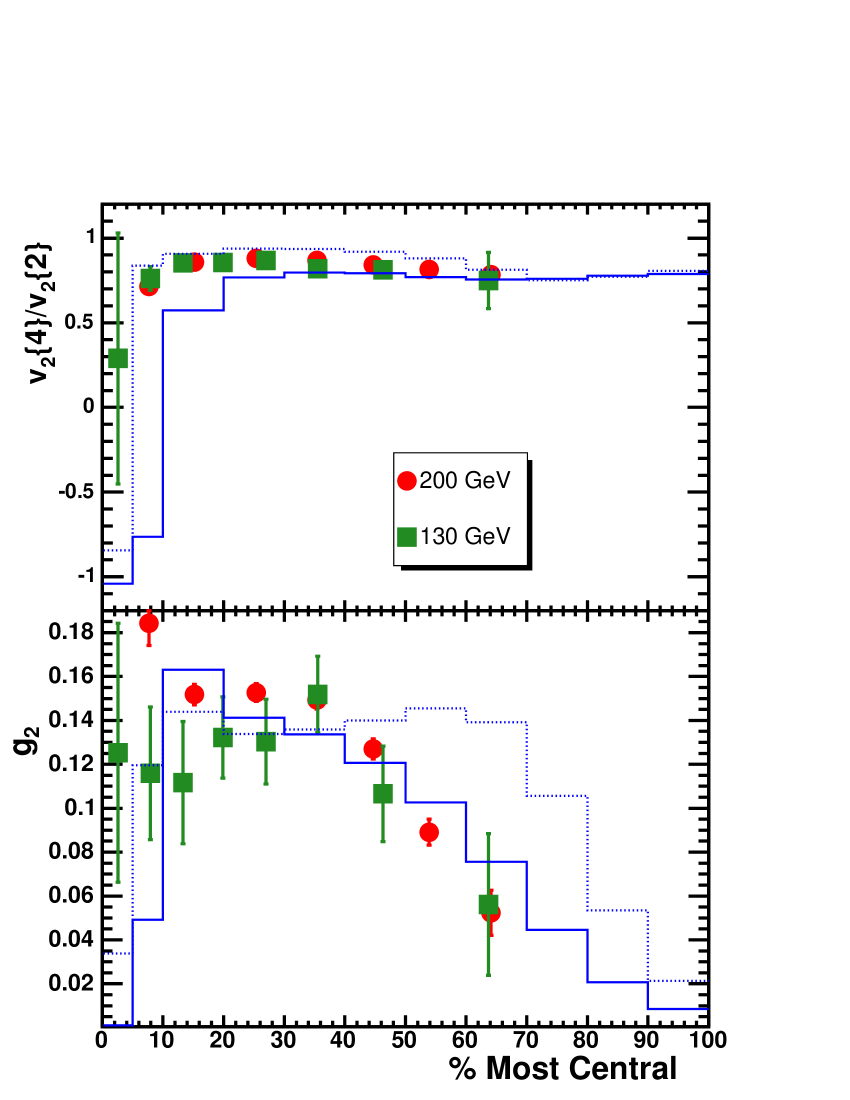
Figure 32: (color online). Upper panel: The ratio $v_{2}\{4\}/v_{2}\{2\}$ for charged hadrons as a function of centrality. The lines are a Monte Carlo Glauber model calculation of ${\varepsilon}_{2}\{4\}/{\varepsilon}_{2}\{2\}$. Lower panel: The nonflow parameter, $g_{2}$, as a function of centrality. The lines are a Monte Carlo Glauber model calculation of $N_{WN}\cdot(v_{2}/{\varepsilon})^{2}\cdot({\varepsilon}_{2}^{2}\{2\}-{\varepsilon}_{2}^{2}\{4\})$. In both panels the solid lines assume nucleons, while the dotted lines assume quarks.

Fluctuations of the true $v_{2}$ can lead to an increase in the $v_{2}\{2\}$ values and an equal decrease in the $v_{2}\{4\}$ values STARcumulants . In Ref. epsilonMC initial spatial eccentricity fluctuations are calculated in a Monte Carlo Glauber (MCG) model and their possible effect on the determination of elliptic flow is estimated. To do this they take

$$({\varepsilon}\{2\})^{2} = \langle{\varepsilon}^{2}\rangle$$

$$({\varepsilon}\{4\})^{4} = 2\langle{\varepsilon}^{2}\rangle^{2}-\langle{\varepsilon}^{4}\rangle,$$

where the averages are over events and ${\varepsilon}$ is the eccentricity which will be defined in Eq. (15). The physics assumption is that $v_{2}\propto{\varepsilon}$. Figure 32 top panel shows ${\varepsilon}\{4\}/{\varepsilon}\{2\}$ for the quark and nucleon MCG. As with nonflow, this ratio is smaller than unity over the whole centrality range, with the largest suppression for the nucleon MCG. The 130 GeV STARcumulants and 200 GeV data are in between the calculated values, and are closer to the nucleon (quark) MCG results for peripheral (central) collisions. When the fluctuations are small it can be shown that $v_{2}\{4\}\approx v_{2}\{6\}$, and from Fig. 30 it is clear that the data indeed support this.

Figure 32 bottom panel shows the calculated $g_{2}$ due to eccentricity fluctuations epsilonMC . In contrast to expectations from nonflow, which would predict a constant value of $g_{2}$ vs. centrality, the eccentricity fluctuations reproduce the observed drop of about a factor 3 vs. centrality as observed in the data.

Thus it appears that either nonflow or fluctuations can explain the two bands in Fig. 29. Most probably it is some of both. Since nonflow effects and fluctuations raise the two-particle correlation values, and fluctuations lower the multi-particle correlation values, the truth must lie between the lower band and the mean of the two bands. At the moment we can only take the difference of the bands as an estimate of our systematic error.

VI Model comparisons

This section compares the experimental results with model calculations. Measurements of event anisotropy, especially elliptic flow $v_{2}$, are sensitive to the early collision dynamics sorge97 ; sorge99 ; ollitrault92 ; shuryak01 . Extracting physics from the huge set of presented data is done via a variety of methods, ranging from transport models which include really quite detailed (and diverse) descriptions of the sub-nuclear dynamics, to hydrodynamic models which make simplifying assumptions (zero mean free path and thermalization) rendering all dynamic details irrelevant and focusing all physics on the equation of state. We first consider schematic concepts like coalescence which propose an underlying nature of the flowing constituents and allow observable tests of scaling relations implied by those concepts. Finally we use a simple Blast Wave parameterization, which tries to see whether a consistent picture of all data can be achieved and to identify what are the required driving features (like geometric anisotropy at freeze-out, etc).

VI.1 Coalescence of constituent quarks

Models of hadron formation by coalescence or recombination of constituent quarks successfully describe hadron production in the intermediate $p_{t}$ region ($1.5\mbox{$\ <\ $}p_{t}\mbox{$\ <\ $}5$ $\mathrm{GeV}/c$) Adler:2003kg ; STAR_Rcp ; reco . These models predict that at intermediate $p_{t}$, $v_{2}$ will approximately scale with the number of constituent quarks ($n$) with $v_{2}/n$ vs. $p_{t}/n$ for all hadrons falling on a universal curve. When hadron formation is dominated by coalescence, this universal curve represents the momentum-space anisotropy of constituent quarks prior to hadron formation. This simple scaling, however, neglects possible higher harmonics and possible differences between light and heavy quark flow.

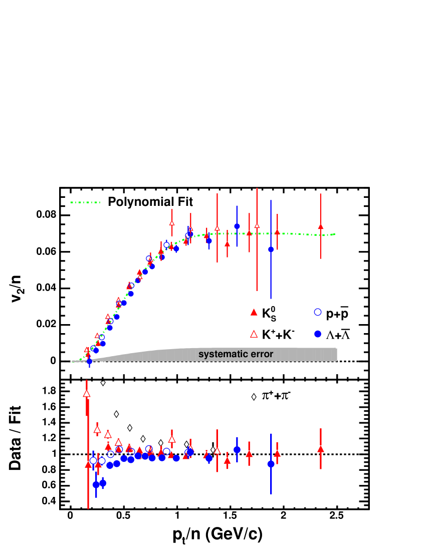
Figure 33: (color online). Top panel: Identified particle $v_{2}$ from minimum bias collisions. The vertical axis and horizontal axis have been scaled by the number of constituent quarks ($n$). Pions are not plotted. A polynomial curve is fit to the data. The possible systematic error is indicated by the gray band. Bottom panel: The ratio of $v_{2}/n$ to the fitted curve.

Figure 33 (top panel) shows $v_{2}$ vs. $p_{t}$ for the identified particle data of Fig. 10, where $v_{2}$ and $p_{t}$ have been scaled by the number of constituent quarks ($n$). A polynomial function has been fit to the shown scaled values. To investigate the quality of agreement between particle species, the data from the top panel are scaled by the fitted polynomial function and plotted in the bottom panel. For $p_{t}/n\mbox{$\ >\ $}0.6$ $\mathrm{GeV}/c$, the scaled $v_{2}$ of $\mathrm{K}^{0}_{S}$ , $K^{\pm}$, p+$\mathrm{\overline{p}}$, and $\Lambda+\overline{\Lambda}$ lie on a universal curve within statistical errors. The pion points, however, deviate significantly from this curve even above 0.6 $\mathrm{GeV}/c$. This deviation may be caused by the contribution of pions from resonance decays decayv2 . Alternatively, it may reflect the difficulty of a constituent-quark-coalescence model to describe the production of pions whose masses are significantly smaller than the assumed constituent-quark masses reco .

At the end of Sec. V.2 we estimated that the $v_{2}$ values from two-particle correlations could be systematically high by between about 10 to 20%. This was based on the integrated values for charged particles and we do not know yet how this varies with $p_{t}$ and particle type. However, to indicate this estimated systematic error a shaded band of 10% is shown in Fig. 33 (top panel).

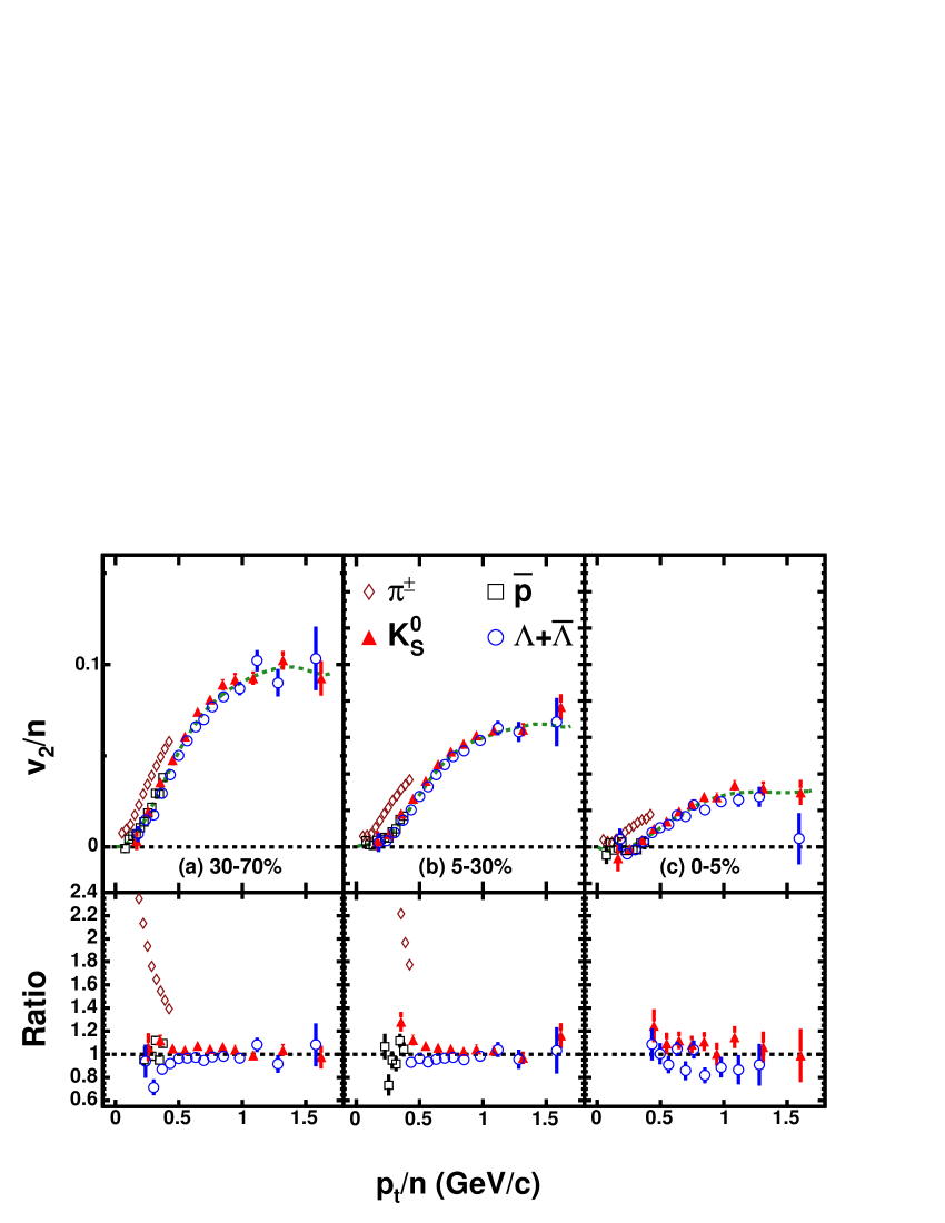
Figure 34: (color online). Top panels: The $v_{2}$ of $\pi^{\pm}$, $\overline{p}$, $\mathrm{K}^{0}_{S}$ , and $\Lambda+\overline{\Lambda}$ from three centrality bins (30–70%, 5–30%, and 0–5% of the collision cross section) scaled by the number of constituent quarks ($n$) vs. $p_{t}/n$. Polynomial curves are fit to the data excluding the pions. Bottom panel: The ratios of $v_{2}/n$ to the fitted curves.

The $v_{2}/n$ of $\pi^{\pm}$, $\overline{p}$, $\mathrm{K}^{0}_{S}$ , and $\Lambda+\overline{\Lambda}$ from three centrality intervals are shown in the top panels of Fig. 34. The $\mathrm{K}^{0}_{S}$ and $\Lambda+\overline{\Lambda}$ values are from Ref. STAR_Rcp . In the bottom panels, the ratios to the fitted curves are shown. The most central data (0–5%) are thought to be affected by nonflow correlations (See Sec. V). For the 30–70% and 5–30% centrality intervals, the $v_{2}$ of $\overline{p}$, $\mathrm{K}^{0}_{S}$ and $\Lambda+\overline{\Lambda}$ agree with constituent-quark-number scaling for the expected $p_{t}/n$ range above 0.6 $\mathrm{GeV}/c$ to within 10%.

Figure 10 showed that the data for the heavier baryons seem to cross over the data for the mesons at sufficiently high $p_{t}$. The data in Fig. 8 are consistent with this. In the low $p_{t}$ region the heavier particles have lower $v_{2}$ values as expected for the mass ordering from hydrodynamics. In the intermediate $p_{t}$ coalescence plateau region the three quark baryons have a larger $v_{2}$ than the two quark mesons. Thus the experimentally observed cross-over is thought to be due to a change in the particle production mechanism.

Table 3: The ratio $v_{4}/v_{2}^{2}$ for all $p_{t}$ and only for $p_{t}/n>0.6$ $\mathrm{GeV}/c$.

	all $p_{t}$	$p_{t}/n>0.6$ $\mathrm{GeV}/c$
$h^{\pm}$	1.17 $\pm$ 0.01	1.14 $\pm$ 0.02
$\pi^{\pm}$	1.19 $\pm$ 0.04
$\mathrm{K}^{0}_{S}$	3.1 $\pm$ 1.2	2.5 $\pm$ 1.3
$\overline{p}$	1.46 $\pm$ 0.53
$\Lambda+\overline{\Lambda}$	0.97 $\pm$ 0.18	0.87 $\pm$ 0.22

From a simple parton coalescence model one can calculate coalescence the observed $v_{4}/v_{2}^{2}$ scaling ratio in terms of the same quantity for the quarks. The relationships between meson ($M$) or baryon ($B$) $v_{4}/v_{2}^{2}$ and quark ($q$) $v_{4}/v_{2}^{2}$ are

$$\left[v_{4}/v_{2}^{2}\right]^{M}_{p_{t}}\approx 1/4+(1/2)\left[v_{4}/v_{2}^{2}\right]^{q}_{p_{t}/2},$$ (11)

and

$$\left[v_{4}/v_{2}^{2}\right]^{B}_{p_{t}}\approx 1/3+(1/3)\left[v_{4}/v_{2}^{2}\right]^{q}_{p_{t}/3}.$$ (12)

These can be rearranged coalescence to relate $v_{4}/v_{2}^{2}$ for mesons and baryons:

$$\left[v_{4}/v_{2}^{2}\right]^{B}_{p_{t}/3}\approx(2/3)\left[v_{4}/v_{2}^{2}\right]^{M}_{p_{t}/2}+1/6.$$ (13)

The observed $v_{4}/v_{2}^{2}$ scaling ratios, which appear to be fairly independent of $p_{t}$ in Figs. 22 (b), 25 and 26, are shown in Table 3. Although in Fig. 33, quark-number scaling is shown to work within errors at $p_{t}/n>0.6$ $\mathrm{GeV}/c$ for all particles except pions, it appears that $v_{4}/v_{2}^{2}$ scaling may be applicable over a wider range of $p_{t}$. Charged hadrons are in the Table but should be used with care because they represent a complicated superposition of baryons and mesons from different values of $p_{t}/n$ where the B/M ratio is strongly dependent on centrality and we cannot even assume that the values are a good estimator for mesons. The kaon values are not accurate enough to test the above equation. Even though the pions are known to deviate from the constituent quark number coalescence predictions, we can calculate with Eq. 13, from the charged pions for the wide $p_{t}$ range, that $v_{4}/v_{2}^{2}$ for baryons should be 0.96 $\pm$ 0.03. This is compatible with the values for anti-protons and $\Lambda+\overline{\Lambda}$ in Table 3. Equation 13 would be valuable for testing the concept of quark coalescence in an equilibrated medium, but the accuracy of the data so far do not allow a conclusion.

If, in addition, one assumes partonScaling ; coalescence that the scaling relation for the partons is

$$v_{4}^{q}=(v_{2}^{q})^{2},$$ (14)

then from Eq. (11) $v_{4}/v_{2}^{2}=1/4+1/2=3/4$. For baryons this ratio from Eq. (12) is $1/3+1/3=2/3$, which is even smaller. But, one can see in Table 3 that experimentally this ratio is close to 1.2 for charged hadrons and pions, so that either the parton scaling relation (Eq. (14)) must have a proportionality constant of about 2, or the simple coalescence model needs improvement.

VI.2 Transport models

Most of the transport model analyses were done for charged hadrons, but we will only compare some of the models with identified hadrons. Microscopic hadronic transport calculations under-predict the absolute amplitude of $v_{2}$ by a factor of 2 to 3. However, most of the observed features, like mass hierarchies in both the low $p_{t}$ region and the meson-baryon order, are seen in hadron transport model calculations bleicher02 . The strength of $v_{2}$ should be sensitive to the density and interaction frequency of the constituents. Indeed, when reducing the hadron formation time, the $v_{2}$ values are found to increase bleicher02 . In addition, the tests with the parton cascade models AMPT zwlin02 and ZPC zpc99 give the correct mass hierarchy but require a large parton cross section in order to mimic the early development of $v_{2}$ at mid-rapidity. In ultra-relativistic nuclear collisions, hadrons may not be the right degrees of freedom to describe the early dynamics. At large values of pseudorapidity, however, the AMPT Ko04 model seems able to describe the $v_{1}$, $v_{2}$, and $v_{4}$ results without the large parton cross sections and string melting. At all pseudorapidities, at the later stage, when particle density becomes dilute, transport effects will become important teaney01 ; bravina04 .

For $v_{4}$ the parton cascade model AMPT partonScaling with string melting and a large parton cross section, does calculate reasonable values. However, the calculated proportionality constant in Eq. (14) is about 1, while our data with a simple coalescence model reco imply it to be about 2.

VI.3 Hydrodynamic models

Azimuthal momentum anisotropies in the final state are generated by particle re-interactions from azimuthal spatial anisotropy in the initial state. In the hydrodynamic framework, these re-interactions are modeled by assuming zero mean free-path and therefore local thermalization. Hydrodynamic calculations have been successful at reproducing previously published data on $v_{2}$ and spectra heinz04 ; kolb04 ; heinz04a .

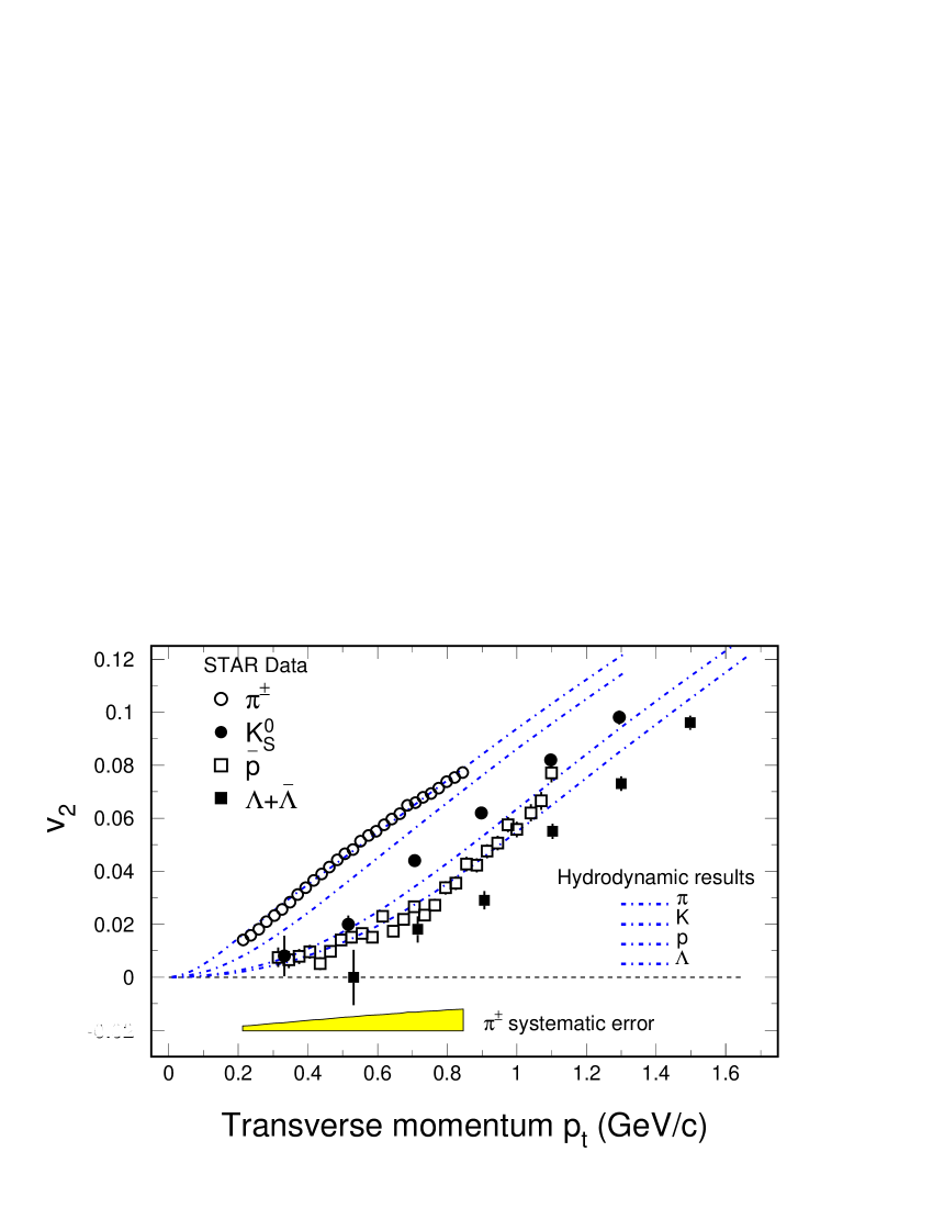
Figure 35: (color online). $v_{2}(p_{t})$ for charged $\pi$, $\mathrm{K}^{0}_{S}$ , $\overline{p}$ and $\Lambda+\overline{\Lambda}$ from minimum bias collisions. Hydrodynamic calculations pasi01 ; pasi03 are shown as dot-dashed lines. The possible systematic error is shown at the bottom.

Hydrodynamic calculations have been shown in Figs. 6, 8, 9, and 10, with reasonable agreement with the $v_{2}$ and $v_{2}\{4\}$ data up to $p_{t}$ of 1-2 $\mathrm{GeV}/c$. Additional results for $v_{2}$ at low $p_{t}$ from minimum bias collisions, are shown in Fig. 35. Results of $\mathrm{K}^{0}_{S}$ and $\Lambda+\overline{\Lambda}$ are from Ref. STAR_Rcp . The hydrodynamic calculations pasi01 ; heinz04 ; pasi03 are consistent with the experimental results considering the systematic errors, such as the matching of the centralities are not included. Also, as described in Sec. V, the data could be 10 to 20% systematically high. To indicate this in the plot a band of 10% of the charged pions is shown. The characteristic hadron mass ordering of $v_{2}$ is seen in the low $p_{t}$ region, where at a given $p_{t}$, the higher the hadron mass the lower the value of $v_{2}$. This supports the hypothesis of early development of collectivity and possible thermalization in collisions at RHIC heinz04 ; heinz04a , although the underlying mechanism for the equilibration process remains an open issue.

As seen in Fig. 33 the observed values of $v_{2}$ saturate and the level of the saturation seems dependent on the number of constituent quarks (n) in the hadron. The saturation value is about $0.07n$ for $p_{t}/n>$ 1 $\mathrm{GeV}/c$. Hydrodynamic calculations do not saturate in this $p_{t}$ region.

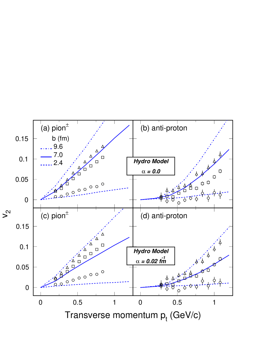
Figure 36: (color online). Charged $\pi$ plots on the left and $\overline{p}$ plots on the right for $v_{2}$ for three centrality bins are shown as a function of $p_{t}$. The data are from centralities 40–50% (open triangles), 20–30% (open squares) and 0–5% (open circles). The corresponding results of a hydrodynamic calculation are shown as dot-dashed lines, solid-lines, and dashed-lines, respectively. Plots on the top are for $\alpha=0$ and plots on the bottom are for $\alpha=0.02\ \rm{fm}^{-1}$. Here $\alpha$ determines the initial velocity kick for the hydrodynamic model calculation kolb02 .

Figure 36 shows the centrality dependence of pion and anti-proton $v_{2}$ compared with hydrodynamic results kolb02 . The three centrality bins shown are described in Table 2. Systematic uncertainties, such as the matching of the centralities, are not included. Also, from the Fig. 29 (b) ratio graph in Sec. V it can be seen that the 0–5% centrality data could be 25% high. An important concern for the 0–5% centrality bin is the fluctuations. Just averaging over the spread in impact parameters in this bin could lower $v_{2}$ a factor of two STARcumulants ; epsilonMC . In the hydrodynamic calculation, the decoupling temperature was set to 100 MeV. In order to fit the $p_{t}$ spectra of (anti-)protons, the hydrodynamic evolution was started with an initial transverse velocity kick of $\tanh(\alpha\cdot r)$, where $\alpha$ is a parameter kolb02 . The results for $v_{2}$ are shown in Fig. 36. For $\alpha=0$, Fig. 36 (a) and (b), neither pion nor anti-proton results can be fitted . For $\alpha=0.02\ {\rm fm}^{-1}$, anti-proton (d) $v_{2}$ can be fitted reasonably well but, for pions (c), the model results still miss the data. It appears that with the initial velocity, there is too much kick for pions at both mid-central and central collisions. Due to their light mass, perhaps pions decouple from the system relatively earlier than protons, as also indicated in the pion interferometry results rhic130hbt . It seems that for the 40–50% centrality data the hydro calculations over-predict the data, which is not surprising for peripheral collisions.

Both Hirano hirano and Heinz and Kolb noTherm explain the fall-off of $v_{2}$ at high $\eta$ as being due to incomplete thermalization. The particle density, $dN/dy$, also falls off in the same way, and at high $\eta$ is similar to that at mid-rapidity at the SPS NA49 , where the flow values are also lower. Possibly, the lower particle density leads to less thermalization, and therefore smaller $v_{2}$ values.

Hydrodynamic inspired fits have been done for spectra heinz93 . Csanád et al. now report results where the authors claim that the resulting $p_{t}$ spectra, interferometry parameters, and anisotropy can all be fitted csanad04 . In particular, they have a fall-off of $v_{2}$ at high $\eta$. But their $v_{1}(\eta)$ has a large wiggle near mid-rapidity which is not observed. They further determined the source parameters and concluded that about 15% of the hadrons are emitted directly from the super-heated region.

So far there have been very few model calculations of $v_{4}$. However, the magnitude and even the sign of $v_{4}$ are more sensitive than $v_{2}$ to initial conditions in the hydrodynamic calculations Kolb_v4 . This calculation predicted $v_{4}/v_{2}^{2}$ to vary from 0.7 to 0.3 going from low to high $p_{t}$, which is about a factor of two lower than observed in the Fig. 22 (b) ratio graph and Table 3. This calculation also predicted a strongly negative $v_{6}$, which is not observed STARv1v4 .

VI.4 Blast Wave models

Blast Wave models parameterize the coordinate and momentum freeze-out configuration generated in hydrodynamic calculations. In a self-consistent hydrodynamic calculation, this configuration is determined by the Equation of State and freeze-out prescription; in Blast Wave calculations, parameters of the distribution may be varied arbitrarily to fit the data. In this sense, Blast Wave is a “toy” model useful mainly to characterize the data and determine the magnitude of thermal (random) motion, collective motion, geometry, etc. The model also provides parameters that can be used to study the evolution of flow varying the initial conditions, which in this paper is achieved by varying centrality.

The present paper uses two versions of the Blast Wave parameterization. In the first one, all particles are emitted from a surface shell boosted by a constant flow velocity STARPID ; STARv4 . In the second one, particles are emitted from a filled elliptic cylinder boosted perpendicular to the surface of the cylinder, and with a linear transverse rapidity profile inside the cylinder BlastWave . In this paper, unless otherwise specified, Blast Wave fits have referred to the filled elliptic cylinder version.

Figure 37: (color online). Schematic illustration of an elliptical sub-shell of the source. Here, the source is extended in the direction out of the event plane ($R_{y}>R_{x}$). Arrows represent the direction and magnitude of the flow boost. In this example, $\rho_{2}>0$. From Ref. BlastWave .

In recent versions of Blast Wave models, the system is assumed boost-invariant in the beam direction. As suggested in Fig. 37 for the filled elliptic cylinder, the geometry in the transverse direction is a filled ellipse with the major axis aligned with the reaction plane or perpendicular to it. One may quantify the geometrical anisotropy of the system with the eccentricity

$${\varepsilon}\equiv\frac{R^{2}_{y}-R^{2}_{x}}{R^{2}_{y}+R^{2}_{x}},$$ (15)

where the $x$ direction is in the reaction plane. Superimposed on a randomly-directed energy component quantified by a temperature, $T$, each geometrical cell of the system is boosted “outward” by a velocity (flow) field. Here, “outward” indicates the direction normal to the surface of the elliptical shell on which the element sits. The magnitude of the flow field vanishes (by symmetry) at the center of the system and grows linearly with the distance from the center, reaching its maximum at the transverse edge of the system (here assumed to be a sharp, non-diffuse edge). The average value of the flow magnitude is quantified by a parameter $\rho_{0}$. The flow magnitude may be larger (or smaller) for sources emitting in the $x$- versus the $y$-direction; the magnitude of this boost oscillation with azimuthal angle is quantified by the parameters $\rho_{2}$ and $\rho_{4}$. In Fig. 37, a larger in-plane than out-of-plane boost (corresponding to $\rho_{2}>0$) is suggested by the longer boost angles in-plane.

Several parameters of the system affect $v_{2}$. Obviously, the larger the magnitude of $\rho_{2}$, the larger the momentum-space anisotropy. Further, the geometric anisotropy plays a role even if the boost strength is identical in all directions ($\rho_{2}=\rho_{4}=0$), if $R_{y}>R_{x}$ ($R_{y}<R_{x}$) it is clear from Fig. 37 that a greater (lesser) number of elements boost particles into the reaction plane, resulting in anisotropy in azimuthal momentum space. Finally, it is clear that the temperature, $T$, plays a role, since if the random energy component is dominant ($T$ larger than the rest mass), momentum anisotropies will be reduced. An extensive discussion of the interplay between these effects may be found in Ref. BlastWave .

To summarize, the free parameters of the fits in the shell case are $T$, $\rho_{0}$, $\rho_{2}$, $\rho_{4}$, $s_{2}$ and $s_{4}$, where $T$ is the temperature parameter, the $\rho_{n}$ are the harmonic coefficients of the source element boost in transverse rapidity, and the $s_{n}$ are the harmonic coefficients of the source density which boosts into a particular direction. In previous parameterizations STARPID where there was no $\rho_{4}$, $\rho_{2}$ was called $\rho_{a}$. In the filled ellipse case the free parameters are $T$, $\rho_{0}$, $\rho_{2}$, $\rho_{4}$, $R_{x}$, and $R_{y}$, where $R_{x}$ is the in-plane radius of the ellipse and $R_{y}$ is kept constant at a non-zero value. In fitting data with a surface shell model $\rho_{0}$ is about $2/3$ as large as for a solid cylinder with a linear profile. The eccentricity is approximately equal to $2s_{2}$. For an ellipse, the parameter $s_{4}$ is approximately equal to $s_{2}^{2}$. The actual equations used are given in Appendix A.

First we verified that the hydrodynamic calculations reported in Ref. Kolb_v4 can be successfully fit by the Blast Wave model with reasonable parameters: $T$ = 93 MeV, $\rho_{0}$ = 0.91, $\rho_{2}$ = 0.080, $\rho_{4}$ = 0.0017, ${\varepsilon}$ = 0.122. Since the hydro had no error bars there is no $\chi^{2}/ndf$. While spectra and $v_{2}$ are well reproduced up to $p_{t}=$ 1.5–2 $\mathrm{GeV}/c$, the $p_{t}$ dependence of $v_{4}$ appears quadratic in the Blast Wave, while rather linear in the hydrodynamic calculation.

We have seen in Fig. 7 that the Blast Wave parameterization does a good job at simultaneously reproducing pion, kaon and anti-proton $v_{2}$. The fits are performed simultaneously to spectra as well as on $v_{2}$ and $v_{4}$, in order to be over-constrained. Pion, kaon and proton spectra (not shown) are well reproduced. Because spectra have typically more data points and smaller error bars, both $T$ and $\rho_{0}$ can be determined, while $\rho_{2}$, $\rho_{4}$, and ${\varepsilon}$ are constrained by the $v_{n}$. The total $\chi^{2}$ per degree of freedom varies for different centralities around an average value of 56/65, without exhibiting any specific dependences. The average $\chi^{2}$ per data point is 14/6 for pions, 7/4 for kaons and 17/10 for protons. When looking at individual data sets (e.g pion $v_{2}$, proton spectra), the $\chi^{2}$ is compared to the number of data points because the degrees of freedom can only be calculated including all the data points as each parameter is constrained by more than one data set. Because the $v_{2}$ error bars are small (less than 5%) compared to the spectra error bars (between 5 and 10%) the total $\chi^{2}$ is dominated by the contributions from the $v_{2}$ results. The calculation fits the peculiar negative values of the anti-proton $v_{2}$ in Fig 7 (c) in central collisions with $p_{t}$ below 0.5 $\mathrm{GeV}/c$. This feature is reproduced when $\rho_{2}$ is significant while the thermal velocity is small. In this case the flow boost is strong enough that it suppresses the low $p_{t}$ anti-proton emission in-plane compared to out-of-plane pasi01 . When the eccentricity is sufficiently large this phenomenon does not take place. The pion $v_{2}(p_{t})$ data points in Fig 7 (a) are similar in the three most peripheral bins. However, the anti-proton values are not, and thus meaningful fits are still possible. The $p_{t}$ ranges in $\mathrm{GeV}/c$ used for the Blast Wave fits where the data had reasonable error bars were 0.4 to 1.0 for pions, 0.15 to 0.5 for kaons, and 0.3 to 1.1 for anti-protons.

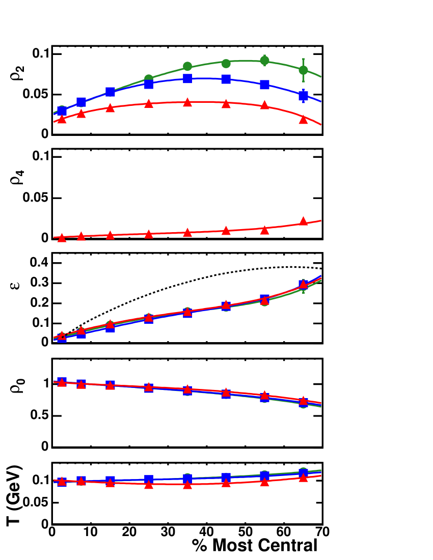
Figure 38: (color online). The Blast Wave parameters $\rho_{2}$, $\rho_{4}$, ${\varepsilon}$, $\rho_{0}$ and T plotted vs. centrality. The circles are for pions from a two-particle cumulant analysis, the squares for pions from a standard event-plane analysis, and the the triangles for charged hadrons from a standard analysis. The lines are polynomial fits. In the middle panel the initial geometrical eccentricity is also plotted as a dashed line. The actual parameter values are available at http://www.star.bnl.gov/central/publications/ .

The Blast Wave parameters obtained from fitting $v_{2}$ and $v_{4}$ data are shown in Fig. 38. They provide a good way to systematize a large amount of experimental data. It should be emphasized that other formulations of the Blast Wave model would give different fit parameters tomasik . As the parameters $T$ and $\rho_{0}$ are constrained mostly by spectra, they agree with the values published STARspectra200 . $\rho_{2}$ and ${\varepsilon}$ are fully constrained by the $v_{2}$ data. $\rho_{2}$ reaches a maximum in the centrality region 30–60%. This is easily understood recalling that in this centrality region, the initial spatial azimuthal anisotropy of the system is large, while the initial energy density is still large enough to trigger a significant collective expansion. This expansion is clearly visible comparing the initial and final eccentricities. The system spatial deformation is a maximum in the region where the azimuthal push quantified by $\rho_{2}$ is a maximum. Thus, the Blast Wave parameterization provides an intuitive self-consistent description of the data.

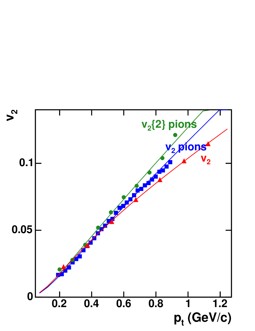
Figure 39: (color online). For centrality 20–30% we show $v_{2}\{2\}$ for pions (circles), $v_{2}$ for pions (squares), and $v_{2}$ for charged hadrons (triangles). The solid lines are Blast Wave fits.

For one centrality we show in Fig. 39 the charged hadron results from this standard event-plane analysis, together with pion results for a standard analysis and a two-particle cumulant analysis. As shown in Sec. V, the integrated two-particle cumulant $v_{2}\{2\}$ values are usually 5% higher than the standard $v_{2}$ values. The charged hadron values are somewhat smaller than the pion values, because of the presence of protons. Even though the flow values are fairly close, the $\rho_{2}$ fit parameters shown in Fig. 38 differ appreciably. This is because the ${\varepsilon}$ values come out the same and the small differences in the $v_{2}$ values are all forced into the $\rho_{2}$ values. It appears that the ${\varepsilon}$ values are at least half as large as the initial eccentricities of the overlap region.

Both hydrodynamic calculations and Blast Wave fits can well reproduce transverse momentum spectra and second-harmonic anisotropy ($v_{2}$). However, as mentioned above, hydrodynamic calculations do not agree with measured values of $v_{4}$. The question, then, is whether Blast Wave parameters may be adjusted to simultaneously fit $v_{2}$ and $v_{4}$, hopefully providing useful feedback to theorists doing the hydrodynamic calculations. Blast Wave fits to $v_{4}$ are shown in Fig. 24.

Even with only second-harmonic anisotropies in flow strength and spatial geometry, fourth-harmonic momentum-space anisotropies ($v_{4}$) are produced in Blast Wave calculations. Thus it is possible that one could generate $v_{4}$ without any fourth harmonic anisotropy $\rho_{4}$ in Eq. (16) coalescence . Using the surface shell Blast Wave model, we have fit the $v_{2}$ data using only $\rho_{2}$ and $s_{2}$, and then calculated $v_{4}$ as shown in Fig. 22 as the dashed lines. The calculated $v_{4}$ values are much too small, indicating that a real fourth harmonic term is necessary. Then we allowed $\rho_{4}$ and $s_{4}$ to vary as well and obtained the fits shown in Fig. 22 as solid lines. The fact that these parameters are significant suggests that the spatial distribution of the system initial state has a significant fourth harmonic component, which translates into a fourth harmonic flow oscillation.

VII Conclusions

All the presently available STAR data for anisotropic flow in Au+Au collisions at $\mbox{$\sqrt{s_{\mathrm{NN}}}$}=200$ GeV are presented for charged particles and for identified species. Agreement between flow data for STAR and other RHIC experiments is good. New evidence confirms our earlier finding that elliptic flow is in-plane at RHIC. $v_{2}$ as a function of pseudorapidity is not flat, but confirmed to be bell shaped. A detailed comparison of flow analysis methods, shows that either nonflow effects or fluctuations can explain the difference between $v_{2}$ from two-particle correlation results and multi-particle correlation results. The mass dependence of $v_{2}$ at low $p_{t}$ follows the pattern predicted by hydrodynamic models, but a transition to a behavior consistent with quark coalescence at higher $p_{t}$ is observed. For identified particles, $v_{2}$ scales with the number of constituent quarks, $n$, within errors above $p_{t}/n\sim 0.6$ $\mathrm{GeV}/c$ for charged and neutral kaons, for anti-protons, and for $\Lambda+\overline{\Lambda}$  hyperons. This supports the picture of hadron production via coalescence of constituent quarks involved in collective anisotropic motion. If confirmed it would be a strong argument for the deconfinement reached in the system. Only pions deviate from this behavior, which partially can be explained by the large resonance decay contribution to pion production, and by the light pion mass. For the higher flow harmonics of order $n$, $v_{n}$ scales with $v_{2}^{n/2}$, consistent with quark coalescence. However, the ratio $v_{4}/v_{2}^{2}$ is unexpectedly large. Some hadronic transport models are a factor of 2–3 lower than the data, but others achieve reasonable agreement. However, hydrodynamic model calculations provide the best predictions for $v_{2}$ compared with data. The characteristic collectivity feature – hadron mass dependence in the low $p_{t}$ region – is observed. Hydrodynamic models seem to work for minimum bias data but not for centrality selected pion and anti-proton data. The discrepancy for the central collision data may be due to nonflow effects and fluctuations in the data, and for the peripheral collisions from a failure of hydrodynamics. Perhaps, more work is needed to improve the hydrodynamic fits, especially for the different centrality bins, in order to make the case for early thermalization of collisions at RHIC. Awaiting further theoretical input or explanation are a number of STAR results, such as the large $v_{2}$ at high $p_{t}$ STARhighPtV2Corr and the $v_{4}$ observations. $v_{4}$ is highly sensitive to initial conditions and the equation of state used in hydrodynamic calculations, and therefore a challenge to all model descriptions. The data were systematized with fits to a Blast Wave model. The Blast Wave framework is capable of describing the large volume of experimental data up to $p_{t}$ of 1 or 2 $\mathrm{GeV}/c$ using a relatively small set of fit parameters in each centrality interval, and the fit parameters are found to vary smoothly with centrality.

VIII Acknowledgments

We thank the RHIC Operations Group and RCF at BNL, and NERSC at LBNL for their support. This work was supported in part by the HENP Divisions of the Office of Science of the U.S. DOE; the U.S. NSF; the BMBF of Germany; IN2P3, RA, RPL, and EMN of France; EPSRC of the United Kingdom; FAPESP of Brazil; the Russian Ministry of Science and Technology; the Ministry of Education and the NNSFC of China; Grant Agency of the Czech Republic, FOM and UU of the Netherlands, DAE, DST, and CSIR of the Government of India; Swiss NSF; and the Polish State Committee for Scientific Research.

Appendix A Blast Wave equations

In both the surface shell and the filled elliptic cylinder cases the transverse rapidity parameterization is extended to account for a possible fourth harmonic anisotropy:

$$\rho(\phi_{b})=\rho_{0}+\rho_{2}\cos(2\phi_{b})+\rho_{4}\cos(4\phi_{b}),$$ (16)

where the flow magnitude and anisotropy are accounted for by the $\rho_{n}$ parameters and $\phi_{b}$ is the azimuthal angle of the boost source element defined with respect to the reaction plane, as shown in Fig. 37.

The distribution of source elements relative to $\phi_{b}$ in the case of a surface shell is written including 2^nd and 4^th harmonic azimuthal anisotropy quantified by the $s_{2}$ and $s_{4}$ parameters respectively:

$$\Omega(\phi_{b})=1+2s_{2}\cos(2\phi_{b})+2s_{4}\cos(4\phi_{b})$$ (17)

When $s_{2}$ is positive more particles are boosted in-plane than out-of-plane. In the case of a filled ellipse, the boost direction ($\phi_{b}$) is assumed to be perpendicular to the freeze-out surface, which leads to a relationship between the space and boost azimuthal angles of the emitted particles

$$\tan(\phi_{s})=(R_{y}/R_{x})^{2}\tan(\phi_{b}),$$ (18)

with $R_{x}$ and $R_{y}$ the in-plane and out-of-plane radii, respectively. For the $v_{n}$ analysis $R=(R_{x}^{2}+R_{y}^{2})^{1/2}$ is an arbitrary radius, but when interferometry data are also fit, the units become significant. The system is bounded within an ellipse such as $\Omega(r,\phi_{s})=\theta(\tilde{r}(\phi_{s}))$ with $\theta$ the step function and

$$\tilde{r}(\phi_{s})=\sqrt{(r\cos(\phi_{s})/R_{x})^{2}+(r\sin(\phi_{s})/R_{y})^{2}}.$$ (19)

In the filled ellipse case there is no explicit 2^nd and 4^th harmonic parameterization of the spatial distribution of the particle emitting source because it is done implicitly by the ellipse parameterization. A profile, linear in transverse rapidity is used in the filled ellipse case:

$$\rho(r,\phi_{b})=(\rho_{0}+\rho_{2}\cos(2\phi_{b})+\rho_{4}\cos(4\phi_{b}))~{}\tilde{r}(\phi_{b}).$$ (20)

The flow Fourier coefficients are defined by

$$v_{n}=\langle\cos[n(\phi_{p}-\Psi)]\rangle,$$ (21)

where $\phi_{p}$ is the azimuthal angle of the particle momentum. Assuming a Boltzmann plus flow distribution and longitudinal boost invariance, leads to the following expression for $v_{n}$:

$$v_{n}(p_{t})=\frac{\int_{-\pi}^{\pi}d\phi_{s}\int_{0}^{\infty}rdr\int_{0}^{\pi}d\phi_{p}K_{1}(\beta(r,\phi_{b}))\cos(n\phi_{p})e^{\alpha(r,\phi_{b})\cos(\phi_{b}-\phi_{p})}\Omega(r,\phi_{s})}{\int_{-\pi}^{\pi}d\phi_{s}\int_{0}^{\infty}rdr\int_{0}^{\pi}d\phi_{p}K_{1}(\beta(r,\phi_{b}))e^{\alpha(r,\phi_{b})\cos(\phi_{b}-\phi_{p})}\Omega(r,\phi_{s})},$$ (22)

with $\alpha(r,\phi_{b})=(p_{t}/T)\sinh(\rho(r,\phi_{b}))$ and $\beta_{t}(r,\phi_{b})=(m_{t}/T)\cosh(\rho(r,\phi_{b}))$. The relation between $\phi_{b}$ and $\phi_{s}$ is given by Eq. (18). All the integrals are done numerically in the filled ellipse calculation in order to preserve the possibility of computing interferometry radii, even though the formula can be simplified to:

$$v_{n}(p_{t})=\frac{\int_{-\pi}^{\pi}d\phi_{b}\int_{0}^{\infty}rdrK_{1}(\beta(r,\phi_{b}))\cos(n\phi_{b})I_{n}(\alpha(r,\phi_{b}))\Omega(r,\phi_{b})}{\int_{-\pi}^{\pi}d\phi_{b}\int_{0}^{\infty}rdrK_{1}(\beta(r,\phi_{b}))I_{0}(\alpha(r,\phi_{b}))\Omega(r,\phi_{b})}.$$ (23)

For the surface shell case the integral over $r$ is trivial.

Appendix B Derivation of the mixed harmonic event plane method $v_{1}\!\left\{\mathrm{EP}_{1},\mathrm{EP}_{2}\right\}$

Following the discussion in STARv1v4 , we try to reduce the nonflow contribution of the first harmonic signal, $v_{1}$, by subtracting the contributions to the flow vector perpendicular to the reaction plane from the component within the reaction plane. As an estimate of the reaction plane we use the second order event plane $\Psi_{2}$. Correlating the azimuthal angle of a particle, $\phi$, with the first order event plane, $\Psi_{1}$, one then obtains

$$\langle\cos(\phi-\Psi_{2})\cdot\cos(\Psi_{1}-\Psi_{2})-\sin(\phi-\Psi_{2})\cdot\sin(\Psi_{1}-\Psi_{2})\rangle = \langle\cos(\phi+\Psi_{1}-2\Psi_{2})\rangle=$$ (24)

$$\langle\cos(\phi-\Psi_{\mathrm{RP}})\cdot\cos(\Psi_{1}-\Psi_{\mathrm{RP}})\cdot\cos[2(\Psi_{2}-\Psi_{\mathrm{RP}})]\rangle =$$

$$\langle\cos(\phi-\Psi_{\mathrm{RP}})\rangle\cdot\langle\cos(\Psi_{1}-\Psi_{\mathrm{RP}})\rangle\cdot\langle\cos[2(\Psi_{2}-\Psi_{\mathrm{RP}})]\rangle \equiv v_{1}\cdot\mathrm{Res}(\Psi_{1})\cdot\mathrm{Res}(\Psi_{2}).$$ (25)

The factorization in Eq. (25) left-hand side is valid due to the statistical independence of the three factors. While the resolution of the second order event plane, $\mathrm{Res}(\Psi_{2})$, can be obtained by calculating the square-root of the correlation of two subevent planes, the resolution of the first order event plane, $\mathrm{Res}(\Psi_{1})$, can be calculated by considering

$$\langle\cos[2(\Psi_{1}-\Psi_{2})]\rangle =$$

$$\langle\cos^{2}(\Psi_{1}-\Psi_{\mathrm{RP}})\cdot\cos[2(\Psi_{2}-\Psi_{\mathrm{RP}})]\rangle =$$

$$\langle\cos(\Psi_{1}-\Psi_{\mathrm{RP}})\rangle^{2}\cdot\langle\cos[2(\Psi_{2}-\Psi_{\mathrm{RP}})]\rangle =$$

$$\mathrm{Res}^{2}(\Psi_{1})\cdot\mathrm{Res}(\Psi_{2}).$$ (26)

Combining Eqs. (25) right-hand side and (26) yields

$$\mbox{$v_{1}\!\left\{\mathrm{EP}_{1},\mathrm{EP}_{2}\right\}$}=\frac{\langle\cos(\phi+\Psi_{1}-2\Psi_{2})\rangle}{\sqrt{\langle\cos[2(\Psi_{1}-\Psi_{2})]\rangle\cdot\mathrm{Res}(\Psi_{2})}}.$$

This approach is similar to the three-particle correlation method of Borghini, Dinh, and Ollitrault v13 . One obtains their result by replacing the event plane angles $\Psi_{1}$ and $\Psi_{2}$ in the right-hand side of Eq. (24) by emission angles of two particles STARv1v4 .

Experimentally one wants to optimize the resolution of the second order event plane by measuring it in a region $c$ where the signal of $v_{2}$ is strong. This will be around mid-rapidity, preferentially. On the other hand, the influence of nonflow can be reduced even further by measuring the azimuthal angle of the particle in one subevent, $\phi^{a}$, and correlating it to the first order event plane in the other subevent, $\Psi_{1}^{b}$. These subevents might by chosen randomly, or by dividing the acceptance into different regions in pseudorapidity. Since only half of all particles are used to determine each $\Psi_{1}^{a}$ and $\Psi_{1}^{b}$, the statistical errors are increased by a factor of $\sqrt{2}$ compared to the three-particle cumulant method $v_{1}\{3\}$. The final observable looks like this:

$$\mbox{$v_{1}\!\left\{\mathrm{EP}_{1},\mathrm{EP}_{2}\right\}$}=\frac{\langle\cos(\phi^{a}+\Psi_{1}^{b}-2\Psi_{2}^{c})\rangle}{\sqrt{\langle\cos(\Psi_{1}^{a}+\Psi_{1}^{b}-2\Psi_{2}^{c})\rangle\cdot\mathrm{Res}(\Psi_{2}^{c})}}.$$

In our case each particle azimuth was correlated to the first order event plane determined in the other subevent within the FTPCs, and to the second order event plane measured in the TPC.

References

- (1) W. Reisdorf and H.G. Ritter, Annu. Rev. Nucl. Part. Sci. 47, 663 (1997).
- (2) For an overview, see Proc. of Quark Matter 2004, J. Phys. G: Nucl. Part. Phys. 30 (2004).
- (3) RIKEN BNL Research Center Proceedings, vol. 62: New Discoveries at RHIC — The Strongly Interacting Quark-Gluon Plasma, BNL-72391-2004 (2004).
- (4) M. Gyulassy, arXiv: nucl-th/0405013.
- (5) STAR Collaboration, C. Adler , Phys. Rev. Lett. 90, 032301 (2003).
- (6) STAR Collaboration, J. Adams , Phys. Rev. Lett. 93, 252301 (2004).
- (7) M. Anderson , Nucl. Instrum. Meth. A 499, 659 (2003).
- (8) K.H. Ackermann , Nucl. Instrum. Meth. A 499, 713 (2003).
- (9) A. Braem , Nucl. Instrum. Meth. A 499, 720 (2003); B. Lasiuk , Nucl. Phys. A 698, 452c (2002).
- (10) STAR Collaboration, C. Adler , Phys. Rev. Lett. 89, 202301 (2002).
- (11) Mike Miller, PhD dissertation, Yale University (2003).
- (12) STAR Collaboration, C. Adler , Phys. Rev. Lett. 87, 182301 (2001).
- (13) Aihong Tang, PhD dissertation, Kent State University (2002), http://phys.kent.edu/PhDdiss/ .
- (14) W.S. Deng, PhD dissertation, Kent State University (2002); B.E. Norman, PhD dissertation, Kent State University (2003), http://phys.kent.edu/PhDdiss/ .
- (15) STAR Collaboration, C. Adler , Phys. Rev. Lett. 89, 132301 (2002).
- (16) STAR Collaboration, J. Adams , Phys. Rev. Lett. 92, 182301 (2004).
- (17) STAR Collaboration, J. Castillo, J. Phys. G: Nucl. Part. Phys. 30, S1207 (2004).
- (18) A.M. Poskanzer and S.A. Voloshin, Phys. Rev. C58, 1671 (1998).
- (19) STAR Collaboration, K.H. Ackermann , Phys. Rev. Lett. 86, 402 (2001).
- (20) STAR Collaboration, J. Adams , Phys. Rev. Lett. 92, 052302 (2004).
- (21) N. Borghini, P.M. Dinh, and J.-Y. Ollitrault, Phys. Rev. C64, 054901 (2001).
- (22) STAR Collaboration, C. Adler , Phys. Rev. C66, 034904 (2002).
- (23) STAR Collaboration, J. Adams , Phys. Rev. Lett. 92, 062301 (2004).
- (24) STAR Collaboration, A.H. Tang, J. Phys. G: Nucl. Part. Phys. 30, S1235 (2004), arXiv: nucl-ex/0403018.
- (25) STAR Collaboration, M.D. Oldenburg, arXiv: nucl-ex/0403007.
- (26) STAR Collaboration, A.M. Poskanzer, J. Phys. G: Nucl. Part. Phys. 30, S1225 (2004), arXiv: nucl-ex/0403019.
- (27) N. Borghini, P.M. Dinh, and J.-Y. Ollitrault, Phys. Rev. C66, 014905 (2002).
- (28) N. Borghini, P.M. Dinh, and J.-Y. Ollitrault, arXiv: nucl-ex/0110016.
- (29) PHOBOS Collaboration, M. Belt Tonjes, J. Phys. G: Nucl. Part. Phys. 30, S1243 (2004); arXiv: nucl-ex/0403025; S. Manly, arXiv: nucl-ex/0405029; B.B. Back, arXiv: nucl-ex/0407012 (submitted to Phys. Rev. CRapid Comm.); C.M. Vale, arXiv: nucl-ex/0410008.
- (30) D. Molnar and S. A. Voloshin, Phys. Rev. Lett. 91, 092301 (2003); R.C. Hwa and C.B. Yang, Phys. Rev. C67, 064902 (2003); R.J. Fries, B. Müller, C. Nonaka and S.A. Bass, Phys. Rev. C68, 044902 (2003); V. Greco, C.M. Ko and P. Levai, Phys. Rev. C68, 034904 (2003); V. Greco, C.M. Ko and P. Levai, Phys. Rev. Lett. 90, 202302 (2003); R.J. Fries, B. Müller, C. Nonaka and S.A. Bass, Phys. Rev. Lett. 90, 202303 (2003); R.C. Hwa and C.B. Yang, Phys. Rev. C70, 024905 (2004); R.C. Hwa and C.B. Yang, Phys. Rev. C70, 024904 (2004); D. Molnar, arXiv: nucl-th/0408044; S. Pratt and S. Pal, arXiv: nucl-th/0409038.
- (31) P. Huovinen, P.F. Kolb, U.W. Heinz, P.V. Ruuskanen, and S.A. Voloshin, Phys. Lett. B 503, 58 (2001).
- (32) PHENIX Collaboration, S.S. Adler , Phys. Rev. Lett. 91, 182301 (2003).
- (33) STAR Collaboration, J. Adams , Phys. Rev. Lett. 91, 072304 (2003); PHENIX Collaboration, S.S. Adler , Phys. Rev. Lett. 91, 072303 (2003); PHOBOS Collaboration, B.B. Back , Phys. Rev. Lett. 91, 072302 (2003); BRAHMS Collaboration, I. Arsene , Phys. Rev. Lett. 91, 072305 (2003).
- (34) R.C. Hwa and C.B. Yang, Phys. Rev. Lett. 93, 082302 (2004).
- (35) PHOBOS Collaboration, B.B. Back , Phys. Rev. Lett. 89, 222301 (2002).
- (36) M. Gyulassy and M. Plümer, Phys. Lett. B 243, 432 (1990); X.N. Wang and M. Gyulassy, Phys. Rev. Lett. 68, 1480 (1992); R. Baier, D. Schiff and B. G. Zakharov, Ann. Rev. Nucl. Part. Sci. 50, 37 (2000).
- (37) STAR Collaboration, J. Adams , Phys. Rev. Lett. 91, 172302 (2003); Phys. Rev. Lett. 91, 072304 (2003).
- (38) STAR Collaboration, C. Adler , Phys. Rev. Lett. 90, 082302 (2003).
- (39) M. Miller and R. Snellings, arXiv: nucl-ex/0312008.
- (40) P.F. Kolb, Phys. Rev. C68, 031902(R) (2003), and private communication.
- (41) S.A. Voloshin and Y. Zhang, Z. Phys. C 70, 665 (1996).
- (42) J.-Y. Ollitrault, Nucl. Phys. A 590, 561c (1995).
- (43) H. Sorge, Phys. Lett. B 402, 251 (1997).
- (44) H. Sorge, Phys. Rev. Lett. 82, 2048 (1999).
- (45) J.-Y. Ollitrault, Phys. Rev. D46, 229 (1992).
- (46) D. Teaney, J. Lauret, and E.V. Shuryak, Phys. Rev. Lett. 86, 4783 (2001).
- (47) PHENIX Collaboration, S.S. Adler , Phys. Rev. Lett. 91, 172301 (2003).
- (48) V. Greco and C.M. Ko, Phys. Rev. C70, 024901 (2004); X. Dong, S. Esumi, P. Sorensen, N. Xu and Z. Xu, Phys. Lett. B 597, 328 (2004).
- (49) P.F. Kolb, L.-W. Chen, V. Greco, and C.M. Ko, Phys. Rev. C69, 051901(R) (2004).
- (50) L.-W. Chen, C.M. Ko, and Z.-W. Lin, Phys. Rev. C69, 031901(R) (2004).
- (51) M. Bleicher and H. Stöcker, Phys. Lett. B 526, 309 (2002).
- (52) Z.-W. Lin and C.M. Ko, Phys. Rev. C65, 034904 (2002); L.-W. Chen and C.M. Ko, arXiv: nucl-th/0409058; Z.-W. Lin, C.M. Ko, B.-A. Li, B. Zhang, and S. Pal, arXiv: nucl-th/0411110.
- (53) B. Zhang, M. Gyulassy, and C.M. Ko, Phys. Lett. B 455, 45 (1999).
- (54) L.-W. Chen, V. Greco, C.M. Ko, and P.F. Kolb, arXiv: nucl-th/0408021.
- (55) D. Teaney, J. Lauret, and E.V. Shuryak, Nucl. Phys. A698, 479 (2002).
- (56) E. Zabrodin, L. Bravina, C. Fuchs, and A. Faessler, Prog. Part. Nucl. Phys. 53, 183 (2004); G. Burau , arXiv: nucl-th/0411117.
- (57) P.F. Kolb and U. Heinz, in “Quark Gluon Plasma 3”, editors: R.C. Hwa and X.N. Wang, World Scientific, Singapore; arXiv: nucl-th/0305084.
- (58) P.F. Kolb, arXiv: nucl-th/0407066.
- (59) U. Heinz, arXiv: nucl-th/0407067.
- (60) P. Huovinen, private communication (2004). =165 MeV, =130 MeV, EoS=Q.
- (61) P.F. Kolb and R. Rapp, Phys. Rev. C67, 044903 (2003).
- (62) STAR Collaboration, C. Adler, , Phys. Rev. Lett. 87, 082301 (2001); PHENIX Collaboration, K. Adcox, , Phys. Rev. Lett. 88, 192302 (2002).
- (63) T. Hirano, Phys. Rev. C65, 011901(R) (2002).
- (64) U. Heinz and P.F. Kolb, J. Phys. G: Nucl. and Part. Phys. 30, S1229 (2004).
- (65) NA49 Collaboration, C. Alt , Phys. Rev. C68, 034903 (2003).
- (66) E. Schnedermann, J. Sollfrank, and U. Heinz, Phys. Rev. C48, 2462 (1993).
- (67) M. Csanád, T. Csörgő, B. Lörstad, and A. Ster, J. Phys. G: Nucl. and Part. Phys. 30, S1079 (2004).
- (68) F. Retiere and M.A. Lisa, Phys. Rev. C70 044907 (2004).
- (69) B. Tomás̆ik, arXiv: nucl-th/0409074.
- (70) STAR Collaboration, J. Adams , Phys. Rev. Lett. 92, 112301 (2004).