1

Abstract

Recent experimental and theoretical advances in investigating electromagnetic meson production reactions in the nucleon resonance region are reviewed. The article gives a description of current experimental facilities with electron and photon beams and presents an unified derivation of most of the phenomenological approaches being used to extract the resonance parameters from the data. The analyses of $\pi$ and $\eta$ production data and the resulting transition form factors for the $\Delta(1232)P_{33}$, N(1535)$S_{11}$, N(1440)$P_{11}$, and N(1520)$D_{13}$ resonances are discussed in detail. The status of our understanding of the reactions with production of two pions, kaons, and vector mesons is also reviewed.

1 Introduction

The quest for understanding the structure and interaction of hadrons has been the motivation of strong interaction physics for decades. The advent of Quantum Chromodynamics (QCD) ^? has led to a general theoretical description of the strong interaction in terms of the fundamental constituents, quarks and gluons. At very high energies, perturbative methods have proven very effective in the description of many processes. However, because of the complexity of the theory, we are still a long way from being able to describe the strong force as it is manifest in the structure of baryons and mesons. The most fundamental approach to resolve this difficulty is to develop accurate numerical simulations of QCD on the Lattice (Lattice QCD)^?. Alternatively, hadron models with effective degrees of freedom have been constructed for interpreting data. For example, near threshold pion-pion scattering, pion-nucleon scattering, and pion photoproduction can be successfully described by chiral perturbation theory^? which is formulated in terms of hadron degrees of freedom and constrained only by the symmetry properties of QCD. The constituent quark model^?,? is another successful, though not fully understood, example. In some cases, the results from these two different theoretical efforts are complementary in understanding the data and making predictions for future experiments.

For heavy quark systems, Lattice QCD (LQCD) can now predict accurate quantities for interpreting the data from, for example, $B$ meson facilities. For light-quark systems, the small quark masses are difficult to implement, and approximations have been necessary in Lattice QCD calculations. Nevertheless, significant progress has been made in calculating some basic properties of baryons, such as masses of ground states, as well as of low lying excited states ^?,?,?,?. Even the first LQCD calculation of the electromagnetic transition form factors from the ground state proton to the first excited state, the $\Delta(1232)$, has been attempted recently^?. However, reliable Lattice QCD calculations for electromagnetic meson production reactions, the subject of this article, seem to be in the distant future. In the foreseeable future, models of hadron structure and reactions will likely continue to play an important role and provide theoretical guidance for experimenters.

The development of hadron models for the nucleon and nucleon resonances ($N^{*}$) has a long history. In the past three decades, the constituent quark model has been greatly refined to account for residual quark-quark interactions due to one-gluon-exchange^?,? and/or Goldstone boson exchange^?,?. Efforts are underway to re-formulate the model within the relativistic quantum mechanics^?,?,?. Conceptually completely different models have also been developed, such as bag models^?, chiral bag models^?,?, algebraic models^?, soliton models^?, color dielectric models^? Skyrme models^?, and covariant models based on Dyson-Schwinger equations^?. With suitable phenomenlogical procedures, most of these models are comparable in reproducing the low-lying $N^{*}$ spectra as determined by the amplitude analyses of elastic $\pi N$ scattering. However they have rather different predictions on the number and ordering of the highly excited $N^{*}$ states. They also differ significantly in predicting some dynamical quantities such as the electromagnetic and mesonic $N$-$N^{*}$ transition form factors. Clearly, accurate experimental information for these $N^{*}$ observables is needed to distinguish these models. This information can be extracted from the data of electromagnetic meson production reactions. In the past few years, such data with high precision have been extensively accumulated at Thomas Jefferson National Accelerator Facility(JLab), MIT-Bates, and LEGS of Brookhaven National Laboratory in the United States, MAMI of Mainz and ELSA of Bonn in Germany, GRAAL of Grenoble in France, and LEPS of Spring-8 in Japan. In this paper we will review these xperimental developments and the status of our understanding of the data accumulated in recent years. Our focus will be on the study of $N^{*}$ excitations. The use of these data for other investigations will not be covered.

It is useful to briefly describe here the recent advances in using the new data to address some of the long-standing problems in the study of $N^{*}$ physics. The first one is the so-called missing resonance problem. This problem originated from the observation that some of the $N^{*}$ states predicted by the constituent quark model are not seen in the baryon spectra determined mainly from the amplitude analyses of $\pi N$ elastic scattering. There are two possible solutions for this problem. First, it is possible that the constituent quark model has wrong effective degrees of freedom of QCD in describing the highly excited baryon states. Other models with fewer degrees of freedom, such as quark-diquark models or models based on alternative symmetry schemes^?, could be more accurate in reproducing the baryon spectra. The second possibility is that these missing resonances do not couple strongly with the $\pi N$ channel and can only be observed in other processes, as suggested by Isgur and Koniuk^? in 1980. Data from the experiments measuring as many meson-baryon channels as possible are needed to resolve the missing resonance problem.

The second outstanding problem in the study of $N^{*}$ physics is that the partial decay widths of baryon resonances compiled and published periodically by the Particle Data Group (PDG) have very large uncertainties in most cases ^?. For some decay channels, such as $\eta N$, $K\Sigma$ and $\omega N$, the large uncertainties are mainly due to insufficient data. But the discrepancies between the results from using different amplitude analysis methods is also a source of the uncertainties. This problem can be resolved only with a sufficiently large data base that allows much stronger constraints on amplitude analyses, and a strong reduction of the model dependence of the extracted partial decay widths as well as other $N^{*}$ parameters. This requires that the data must be precise and must cover very large kinematic regions in scattering angles, energies, and momentum transfers. The data of polarization observables must also be as extensive as possible.

The above two experimental challenges have been met with the operations of the electron and photon facilities mentioned above. These facilities are also equipped with sophisticated detectors for measuring not only the dominant single pion channel but also kaon, vector meson, and two-pion channels. The CEBAF Large Acceptance Spectrometer (CLAS) at JLab is the most complete and advanced detector in the field.

The third long-standing problem is in the theoretical interpretations of the $N^{*}$ parameters listed by the PDG. Most of the model predictions on $N^{*}\rightarrow\gamma N$ helicity are only in a very qualitative agreement with the PDG values. In some cases, they disagree even in signs. One could attribute this to the large experimental uncertainties, as discussed above. However, the well determined empirical values of the simplest and most unambiguous $\Delta\rightarrow\gamma N$ helicity amplitudes are about $40\%$ larger than the predictions from practically all of the hadron models mentioned above. This raises the question about how the hadron models as well as the Lattice QCD calculations are related to the $N^{*}$ parameters extracted from empirical amplitude analyses. We need to evaluate critically their relationships from the point of view of fundamental reaction theory. The discrepancies in the $\Delta(1232)$ region must be understood before meaningful comparisons between theoretical predictions and empirical values can be made. Much progress has been made in this area. The results, as will be detailed in section 5.1, strongly indicate that it is necessary to apply an appropriate reaction theory in making meaningful comparisons of the empirical values from amplitude analyses and the predictions from hadron models and LQCD.

Summing up the above discussions, it is clear that in the absence of a fundamental solution of QCD in the resonance regions, the study of $N^{*}$ excitations needs close collaborations between theoretical and experimental efforts. This is illustrated in Fig. 1. On the theoretical side, we need to use Lattice QCD calculations and/or hadron structure models to predict properties of nucleon resonances, such as the $N$-$N^{*}$ transition form factors indicated in Fig. 1. On the experimental side, we need to accumulate sufficiently extensive and precise data of meson production reactions. We then must develop reaction models for interpreting the data in terms of hadron structure calculations. The development of empirical amplitude analyses of the data is an important part of this task.

Figure 1: Scheme for $N^{*}$ study

In section 2, the current experimental facilities will be reviewed. The general formulation for calculating cross sections of electromagnetic meson production is presented in section 3. Section 4 is devoted to provide a unified derivation of models used in the interpretation of the data. Results are presented in section 5. Concluding remarks and outlook are given in section 6.

2 Experimental Facilities

2.1 Thomas Jefferson National Accelerator Facility

The Thomas Jefferson National Accelerator Facility (JLab) in Newport News, Virginia, operates a CW electron accelerator with energies in the range up to 6 GeV ^?. Three experimental Halls receive highly polarized electron beams with the same, or with different but correlated energies, simultaneously. Beam currents in the range from 0.1 nA to 150 $\mu$A can be delivered to the experiments, simultaneously.

2.1.1 Experimental Hall A - HRS²

Hall A houses a pair of identical focussing magnetic spectrometers ^? with high resolution (HRS²), each with a momentum resolution of $\Delta p/p\sim 2\times 10^{-4}$, one of them is instrumented with a gas Cerenkov counter and a shower counter for the identification of electrons. The hadron arm is instrumented with a proton recoil polarimeter. The detector package allows identification of charged pions, kaons, and protons. A polarized ${}^{3}He$ target is used for experiments that require polarized neutron targets. The HRS² spectrometers have been used to measure the reaction $\vec{e}p\rightarrow e\vec{p}\pi^{\circ}$ in the $\Delta(1232)$ region and to extract various single and double polarization response functions.

2.1.2 Experimental Hall B - CLAS

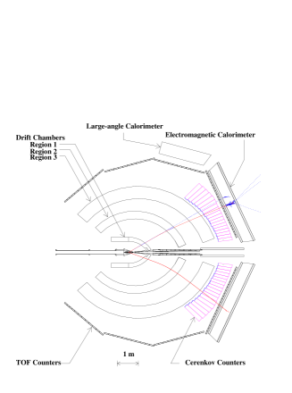
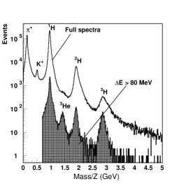
Hall B houses the CEBAF Large Acceptance Spectrometer (CLAS) detector, and a photon energy tagging facility ^?. CLAS can be operated with electron beams and with energy tagged photon beams. The photon beam can be either unpolarized or can be linearly or circularly polarized. The detector system was designed specifically with the detection of multiple particle final states in mind. The driving motivation for the construction of CLAS was the nucleon resonances ($N^{*}$) program, with the emphasis on the study of the $\gamma NN^{*}$ and $\gamma N\Delta^{*}$ transition form factors, and the search for missing resonances. Figure 2 shows the CLAS detector. At the core of the detector is a toroidal magnet consisting of six superconducting coils symmetrically arranged around the beam line. Each of the six sectors is instrumented as an independent spectrometer with 34 layers of tracking chambers allowing for the full reconstruction of the charged particle 3-momentum vectors. Charged hadron identification is accomplished by combining momentum and time-of-flight, and the measured path length from the target to the plastic scintillation counters which surround the entire tracking chambers. Timing resolutions of $\Delta{T}=120-200$ psec (rms) are achieved, depending on the length of the scintillator bar which ranges from 30 cm to 350 cm. Mass and charge number (Z) reconstruction is shown in the left panel of Fig. 3. Protons and pions can be separated for momenta up to 4 GeV/c, and pions and kaons up to about 2 GeV/c. The wide range of particle identification allows to study the complete range of reactions relevant to the $N^{*}$ program. In the polar angle range of up to 70^∘ photons and neutrons can be detected using the electromagnetic calorimeters. The forward angular range from about 10^∘ to 50^∘ is instrumented with gas Cerenkov counters for the identification of electrons.

Figure 2: The CLAS detector at JLab. Left panel: The longitudinal cut along the beam line shows the 3 drift chamber regions, the Cherenkov counter at forward angles, the time-of-flight (TOF) system, and the electromagnetic calorimeters. A simulated event shows an electron (upper) and a positively charged hadron. Right panel: Transverse cut through CLAS. The six superconducting coils provide a six sector structure with independent detectors. A polarized target can be inserted into the large bore near the center.

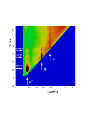
In the $N^{*}$ program, CLAS is often used as a “missing mass” spectrometer, where all final state particles except one particle are detected. The undetected particle is inferred through the overdetermined kinematics, making use of the good momentum and angle resolution. The right panel in figure 3 shows an example of the kinematics covered in the reaction $ep\rightarrow epX$. It shows the invariant hadronic mass $W$ versus the missing mass $M_{X}$. The undetected particles $\pi^{\circ}$, $\eta$, and $~{}\omega$ are clearly visible as bands of constant $M_{X}$. The correlation of certain final states with specific resonance excitations is also clearly seen.

Figure 3: Left panel: Charged particle identification in CLAS. The reconstructed mass/Z(charge number) for positive tracks from a carbon target is shown. Additional sensitivity to high-mass particles is obtained by requiring large energy loss in the scintillators (shaded histogram). Right panel: Invariant mass versus missing mass for $ep\rightarrow epX$ at an electron beam energy of 4 GeV.

2.1.3 Experimental Hall C - HMS and SOS

Hall C houses the high momentum spectrometer (HMS) and the short orbit spectrometer (SOS). The HMS reaches a maximum momentum of 7 GeV/c, while the SOS is limited to about 1.8 GeV/c. The spectrometer pair has been used to measure the $\gamma^{*}N\Delta(1232)$ and $\gamma^{*}NN^{*}(1535)$ transition at high $Q^{2}$ values. For these kinematics the SOS was used as electron spectrometer and the HMS to detect the proton. To achieve a large kinematics coverage, the spectrometers have to be moved in angles, and the spectrometer optics has to be adjusted to accomodate different particle momenta. This makes such a two spectrometer setup most useful for studying meson production at high momentum transfer, or close to threshold. In either case, the Lorentz boost guarantees that particles are produced in a relatively narrow cone around the virtual photon, and can be detected in magnetic spectrometers with relatively small solid angles.

2.2 MAMI-B

The MAMI-B microtron electron accelerator ^? at Mainz in Germany reaches a maximum beam energy of 850 MeV. There are experimental areas for electron scattering experiments with three focussing magnetic spectrometers with high resolution ^?. A two-spectrometer configuration has been used in cross section and polarization asymmetry measurements of $\pi^{\circ}$ electroproduction from protons in the $\Delta(1232)$ region.

Another experimental area is equipped for physics with an energy-tagged photon bremsstrahlung beam ^?. Experimental setups with $BaF_{2}$ crystals (TAPS) have been employed for measurements of differential cross sections for $\pi^{\circ}$ and $\eta$ production and for beam asymmetry measurements using a linearly polarized coherent bremsstrahlung beam.

2.3 MIT-Bates

The Bates 850 MeV linear electron accelerator has been used to study $\pi^{\circ}$ production in the $\Delta(1232)$ region using an out-of-plane spectrometer setup ^?. A set of four independent focussing spectrometers was used to measure various response functions, including the beam helicity-dependent out-of-plane response function. Because of the small solid angles covered by this seteup, a limited range of the polar angles in the center of mass frame of the $p\pi^{\circ}$ subsystem could be covered. These spectrometers are no longer in use, but data are still being analyzed.

2.4 Laser backscattering photon facilities

Electron storage rings built as light sources for material science studies are often used parasitically to produce high energy photons for nuclear physics applications. An intense laser beam is directed tangentially at the electron beam circulating in the storage ring producing high energy Compton backscattered photons in an energy range dependent upon the wavelength of the laser light. While the photon intensities are quite modest, the energy spectrum is peaked at the high energy end providing an efficient source of high energy photons for nuclear physics experiments. The laser light is easily polarized linearly or circularly. In the Compton backscattering process the polarization of the laser light is transferred to the high energy photon beam providing a convenient source of polarized photons.

2.4.1 The Graal Tagged Photon Facility

The Grenoble Synchrotron Light Source facility is used to generate a laser backscattered polarized photon beam of up to 1470 MeV energy for nuclear physics applications. A BGO crystal detector is used for the detection of photons ^? covering a large portion of 4$\pi$. Multi-wire proportional chambers allow charged particle tracking. Particle identification is achieved by time-of-flight measurements at forward angles, and by energy loss measurements at large angles. The large solid angle coverage allows the study of reactions with multiple photons in the final state which is important for nucleon resonance studies in $\pi^{\circ}$ and $\eta$ production ^?.

2.4.2 The LEGS at Brookhaven National Laboratory

Brookhaven National Laboratory operates an electron synchrotron as a light source with an energy of 2.8 GeV/c. A laser backscattered real photon beam with an energy up to 470 MeV is used for nuclear physics experiments ^?. A tagging system measures the energy of the Compton-scattered electron from which the photon energy is inferred. The photon beam is used with an unpolarized hydrogen or nuclear target, and with a polarized HD target ^?. Several arrays of NaI(Tl) crystal detectors have been used to measure Compton scattering and $\pi^{\circ}$ production off protons in the $\Delta(1232)$ region.

2.4.3 LEPS at Spring-8

SPring-8 operates an 8 GeV electron synchrotron near Osaka in Japan. A laser-backscattered, energy-tagged polarized photon beam with an energy up to 2.4 GeV is produced for nuclear and particle physics applications ^?. The LEPS detector consists of a plastic scintillator to detect charged particles produced in the target, an aerogel Cerenkov counter for particle identification, charged-particle tracking counters, a large dipole magnet, and a time-of-flight wall for particle identification. The LEPS detector has been used for $\omega$, and near-threshold $\phi$ production, and for strange particle production.

2.5 Electron Stretcher and Accelerator (ELSA).

The University of Bonn operates a 2.5 GeV electron synchrotron and a stretcher ring and post accelerator to obtain a high duty factor beam and an energy of 3 GeV. Three experimental setups have been used for meson production experiments during the past decade.

2.5.1 The SAPHIR Detector

SAPHIR is a large acceptance detector with 2$\pi$ azimuthal coverage. An external electron beam was used to generate an energy-tagged real photon beam for experiments with the SAPHIR detector ^?. At the core of the detector is a large-gap dipole magnet. Tracking is provided by a central drift chamber located inside the dipole magnet, and additional chambers outside the magnetic field region. Scintillation counters are used for triggering and to provide time-of-flight information for particle identification.

2.5.2 The Crystal Barrel Detector at ELSA

The Crystal Barrel (CB-ELSA) detector was originally used at the LEAR $p\bar{p}$ ring at CERN. The detector was recently brought to ELSA for operation in an energy-tagged bremsstrahlung photon beam ^?. The detector consists of CsI crystals providing nearly full solid angle coverage for neutral particle detection. The main focus is the detection of multiple neutral particle final states.

2.5.3 The Elan Apparatus

The Elan apparatus has been used for studies of single pion electroproduction in the $\Delta(1232)$ region. A focussing magnetic spectrometer detects the scattered electrons, and electromagnetic shower detectors measure photons from $\pi^{\circ}$ decays. Protons and charged pions are detected as well. Charged hadrons are not magnetically analyzed. This setup has been used for measurements of $\pi^{\circ}$ and $\pi^{+}$ in the $\Delta(1232)$ region.

3 General Formalism

The bulk of data from the facilities described in the previous section are from experiments with a single meson and baryon in the final state. We therefore only present the formulation for such reactions. The generalization of the formulation to the cases that the final states are three-body states is straightforward.

We consider the process $N(e,e^{\prime}M)B$ illustrated in Fig. 4. The final meson-baryon states are two-body states, such as $\pi N,\eta N,K\Lambda$, $\omega N$ and $\phi N$. Within the Relativistic Quantum Field Theory, the Hamiltonian density for describing this process can be concisely written as

$$H_{em}(x)=eA_{\mu}(x)[j^{\mu}(x)+J^{\mu}(x)]\,,$$ (1)

where $A_{\mu}$ is the photon field,

$$j^{\mu}(x)=\bar{\psi}_{e}(x)\gamma^{\mu}\psi_{e}(x)$$ (2)

is the lepton current, and the electromagnetic interactions involving hadrons are induced by the hadron current $J^{\mu}$.

Figure 4: One-photon exchange mechanism for meson electroproduction from a nucleon.

With the convention of Bjorken and Drell^?, the Hamiltonian density Eq.(1) leads to

$$<kp^{\prime}\mid\int dxA^{\mu}(x)J_{\mu}(x)\mid qp>=(2\pi)^{4}\delta^{4}(p+q-k-p^{\prime})<kp^{\prime}\mid\epsilon_{\mu}(q)J^{\mu}(0)\mid qp>\,,$$ (3)

where $q$, $p$, $k$, and $p^{\prime}$ are the momenta for the intial photon, intial nucleon, final meson, and final nucleon, respectively, $\epsilon_{\mu}(q)$ is the photon polarization vector. Throughout this paper, we will suppress the spin and isospin indices unless they are needed for detailed explanations.

Figure 5: Kinematics of meson electroproduction reaction.

It is convenient to write

$$<kp^{\prime}\mid\epsilon_{\mu}(q)J^{\mu}(0)\mid qp> = \frac{1}{(2\pi)^{6}}\sqrt{\frac{m_{N}}{E_{N}(p^{\prime})}}\frac{1}{\sqrt{2E_{\pi}(k)}}\epsilon_{\mu}(q)J^{\mu}(k,p^{\prime};q,p)$$ (4)

$$\times \sqrt{\frac{m_{N}}{E_{N}(p)}}\frac{1}{\sqrt{2\omega}}\,.$$

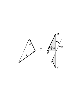
The expression for calculating electromagnetic meson production cross sections can be expressed in terms of $J^{\mu}(k,p^{\prime};q,p)$. For evaluating electroproduction cross sections, it is common and convenient to choose a coordinate system that the virtual photon is in the quantization $z-$direction, and the angle between the $e-e^{\prime}$ plane and $M-B$ plane is $\phi_{M}$, as illustrated in Fig. 5. With some straightforward but lengthy derivations, it is possible to write the differential cross section of $N(\vec{e},e^{\prime}M)B$ reaction in the following form

$$\frac{d^{5}\sigma_{h}}{dE_{e^{\prime}}d\Omega_{e^{\prime}}d\Omega_{M}^{*}} = \Gamma\frac{d\sigma_{h}}{d\Omega^{*}_{M}}\,$$

with

$$\frac{d\sigma_{h}}{d\Omega^{*}_{M}} = \Gamma[\frac{d\sigma_{unpol}}{d\Omega_{M}^{*}}+h\sqrt{2\epsilon(1-\epsilon)}\frac{d\sigma_{LT^{\prime}}}{d\Omega^{*}_{M}}sin\phi_{M}]\,,$$ (5)

where $h$ is the helicity of the incoming electron. The kinematic factors associated with the incoming and outgoing electrons are only contained in the following two variables

$$\epsilon = \{1+\frac{2\mid{\bf q}\mid^{2}}{Q^{2}}tan^{2}\frac{\theta_{e}}{2}\}^{-1}\,,$$ (6)

$$\Gamma = \frac{\alpha K_{H}}{2\pi^{2}Q^{2}}\frac{E_{e}^{\prime}}{E_{e}}\frac{1}{1-\epsilon}\,,$$ (7)

where $K_{H}=\omega-Q^{2}/2m_{N}$ is the virtual photon flux, $\alpha=1/137$ is the electromagnetic coupling constant, $q^{\mu}=(\omega,{\bf q})$ is the momentum of the photon, and $Q^{2}=-q^{2}=\mid{\bf q}\mid^{2}-\omega^{2}$. The incident and outgoing electron energies are related to $q^{\mu}$ by

$$\omega = E_{e}-E^{\prime}_{e}\,,$$ (8)

$$Q^{2} = 4E_{e}E^{\prime}_{e}sin^{2}\frac{\theta_{e}}{2}\,,$$ (9)

where $\theta_{e}$ is the angle between the incident and outgoing electrons.

For investigating $N^{*}$ excitations, the kinematics is often characterized by the initial $\gamma^{*}N$ invariant mass $W$ and $Q^{2}$. For such a choice, the energy transfer is then defined by

$$\omega=\frac{W^{2}+Q^{2}-m_{N}^{2}}{2m_{N}}.$$ (10)

The corresponding electron kinematics for conducting experiments with a given $(Q^{2},W)$ can then be evaluated by using Eqs.(8)-(9).

Note that the differential cross sections in the right-hand side of Eq.(5) is defined in the center of mass (c.m.) frame of the initial $\gamma^{*}N$ and the final $MB$ systems. These quantities must be evaluated in terms of the momenta in that c.m. frame. For the coordinate system chosen as ${\bf q}\parallel\hat{z}$, all momenta needed in calculating $d\sigma/d\Omega^{*}_{M}$ must be transformed by a Lorentz boost with ${\bf\beta}=\hat{z}\mid{\bf q}\mid/(\omega+m_{N})$. In terms of variables $W$ and $Q^{2}$, a momentum $p^{\mu}_{c}$ in the considered c.m. frame is related to a momentum $p^{\mu}$ in the laboratory frame by

$$p^{0}_{c} = \frac{m_{N}+\omega}{W}p^{0}-\frac{\mid{\bf q}\mid}{W}p^{z}\,,$$ (11)

$$p^{x}_{c} = p^{x}\,,$$ (12)

$$p^{y}_{c} = p^{y}\,$$ (13)

$$p^{z}_{c} = -\frac{\mid{\bf q}\mid}{W}p^{0}+\frac{m_{N}+\omega}{W}p^{z}.$$ (14)

Specifically, we have for the virtual photon

$$\mid{\bf q}_{c}\mid = \frac{m_{N}}{W}\mid{\bf q}\mid\,,$$ (15)

$$\omega_{c} = \frac{\omega m_{N}-Q^{2}}{W}\,.$$ (16)

It is easy to see that $Q^{2}={\bf q}^{2}-\omega^{2}={\bf q}^{2}_{c}-\omega^{2}_{c}$

We next present formulae for calculating the c.m. differential cross sections in the right-hand-side of Eq.(5). The unpolarized cross section is given by

$$\frac{d\sigma_{unpol}}{d\Omega^{*}_{M}}=\frac{d\sigma_{T}}{d\Omega^{*}_{M}}+\epsilon\frac{d\sigma_{L}}{d\Omega^{*}_{M}}+\epsilon\frac{d\sigma_{TT}}{d\Omega^{*}_{M}}cos2\phi_{M}+\sqrt{2\epsilon(1+\epsilon)}\frac{d\sigma_{LT}}{d\Omega^{*}_{M}}cos\phi_{M}\,,$$ (17)

where $\sigma_{T}$, $\sigma_{L}$, $\sigma_{TT}$, and $\sigma_{LT}$ are called the transverse, longitudinal, polarization, and interference cross sections. These four cross sections and the $d\sigma_{LT^{\prime}}/d\Omega^{*}$ in Eq.(5) can be written as

$$\frac{d\sigma_{\beta}}{d\Omega^{*}_{M}}=\frac{\mid{\bf k_{c}}\mid}{q^{\gamma}_{c}}M_{\beta}(k_{c},p_{c}^{\prime};q_{c},p_{c})\,,$$ (18)

where $q^{\gamma}_{c}=(W^{2}-m_{N}^{2})/(2m_{N})=K_{H}$ is the effective photon c.m. momentum, $\beta=T,L,TT,LT$ and $LT^{\prime}$, and the c.m. momenta $k_{c}$, $p^{\prime}_{c}$, $q_{c}$, and $p_{c}$ can be calculated from the corresponding momenta in the laboratory frame by using Eqs.(11)-(14). Obviously $q^{\gamma}_{c}=\mid{\bf q_{c}}\mid$ at the photon point $Q^{2}=0$.

The meson production dynamics is contained in $M_{\beta}$ of Eq.(18). They are calculated from various combinations of current matrix elements evaluated on the $\phi_{M}=0$ plane (see Fig.5):

$$M_{T}(k_{c},p_{c}^{\prime};q_{c},p_{c}) = \frac{F}{4}\sum_{spins}[\mid J^{x}(k_{c},p^{\prime}_{c};q_{c},p_{c})\mid^{2}+\mid J^{y}(k_{c},p^{\prime}_{c};q_{c},p_{c})\mid^{2}]_{\phi_{M}=0}$$

$$M_{L}(k_{c},p_{c}^{\prime};q_{c},p_{c}) = \frac{F}{2}\sum_{spns}\frac{Q^{2}}{\omega^{2}}[\mid J^{z}(k_{c},p^{\prime}_{c};q_{c},p_{c})\mid^{2}]_{\phi_{M}=0}$$

$$M_{TT}(k_{c},p_{c}^{\prime};q_{c},p_{c}) = \frac{F}{4}\sum_{spins}[\mid J^{x}(k_{c},p^{\prime}_{c};q_{c},p_{c})\mid^{2}-\mid J^{y}(k_{c},p^{\prime}_{c};q_{c},p_{c})\mid^{2}]_{\phi_{M}=0}$$

$$M_{LT}(k_{c},p_{c}^{\prime};q_{c},p_{c}) = -\frac{F}{2}\sum_{spins}\sqrt{\frac{Q^{2}}{\omega^{2}}}Re\{J^{z}(k_{c},p^{\prime}_{c};q_{c},p_{c})J^{x*}(k_{c},p^{\prime}_{c};q_{c},p_{c})\}_{\phi_{M}=0}$$

$$M_{LT^{\prime}}(k_{c},p_{c}^{\prime};q_{c},p_{c}) = \frac{F}{2}\sum_{spins}\sqrt{\frac{Q^{2}}{\omega^{2}}}Im\{J^{z}(k_{c},p^{\prime}_{c};q_{c},p_{c})J^{x*}(k_{c},p^{\prime}_{c};q_{c},p_{c})\}_{\phi_{M}=0}$$

with

$$F=\frac{e^{2}}{(2\pi)^{2}}\frac{1}{2E_{M}(k_{c})}\frac{m_{N}}{E_{B}(p^{\prime}_{c})}\frac{m_{N}}{E_{N}(p_{c})}\frac{E_{M}(k_{c})E_{B}(p^{\prime}_{c})}{2W}$$ (20)

where $E_{a}(p)=\sqrt{{\bf p}^{2}+m_{a}^{2}}$ with $m_{a}$ denoting the mass of particle $a$.

The differential cross sections of $N(\vec{e},e^{\prime}M)B$ are often expressed in terms of response functions^? $R_{\alpha}$ which are related to the differential cross sections of Eq.(18) by

$$\frac{d\sigma_{T}}{d\Omega^{*}_{M}} = \frac{\mid{\bf k_{c}}\mid}{q^{\gamma}_{c}}R_{T}\,$$

$$\frac{d\sigma_{TT}}{d\Omega^{*}_{M}} = \frac{\mid{\bf k_{c}}\mid}{q^{\gamma}_{c}}R_{TT}\,$$

$$\frac{d\sigma_{L}}{d\Omega^{*}_{M}} = \frac{\mid{\bf k_{c}}\mid}{q^{\gamma}_{c}}\frac{Q^{2}}{\omega_{c}^{2}}R_{L}\,$$

$$\frac{d\sigma_{LT}}{d\Omega^{*}_{M}} = \frac{\mid{\bf k_{c}}\mid}{q^{\gamma}_{c}}\sqrt{\frac{Q^{2}}{\omega_{c}^{2}}}R_{LT}\,$$

$$\frac{d\sigma_{LT^{\prime}}}{d\Omega^{*}_{M}} = \frac{\mid{\bf k_{c}}\mid}{q^{\gamma}_{c}}\sqrt{\frac{Q^{2}}{\omega_{c}^{2}}}R_{LT^{\prime}}.$$

The above formulation can be readily used to calculate various polarization observables with a polarized initial nucleon. For observables with a polarized recoiled final baryon, the situation is more complicated. They have been explicitly derived for pseudo-scalar meson production ^?,?. Formulations for analyzing spin observables of vector meson production were developed in Ref.^?.

We also note that the unpolarized photoproduction cross section is given by $d\sigma_{T}/d\Omega^{*}_{M}$ evaluated at $Q^{2}=0$ and $q^{\gamma}_{c}\rightarrow\mid{\bf q_{c}}\mid$. For polarized photons, one needs to choose an appropriate combination of $J^{x}$ and $J^{y}$. For instance, $d\sigma_{\perp}/d\Omega^{*}_{M}$($d\sigma_{\parallel}/d\Omega^{*}_{M}$)for the photon polarization normal (parallel) to the hadron plane is calculated from keeping only $J^{y}$ ($J^{x}$) contribution and multipling the resulting cross section by a factor of 2. The photon asymmetry is defined as

$$\Sigma_{\gamma}=\frac{\sigma_{\perp}-\sigma_{\parallel}}{\sigma_{\perp}+\sigma_{\parallel}}.$$ (22)

Calculations of other photoproduction polarization observables are given, for example, in the appendix C of Ref.^?.

We next present formulae which are often used in analyzing the production of pseudo-scalar mesons, such as $MB=\pi N,\eta N,KY$. The Lorentz invariance and gauge invariance allow us to write the hadron current matrix elements as

$$\epsilon_{\mu}(q)J^{\mu}(k,p^{\prime};q,p)=\sum_{i=1,6}\bar{u}[({\bf p}^{\prime})A_{i}(s,t,u)M_{i}]u({\bf p})\,,$$ (23)

where $u({\bf p})$ is the Dirac spinor, $A_{i}(s,t,u)$ are Lorentz invariant functions, and $M_{i}$ are independent invariances formed from $\gamma^{\mu}$, $\gamma_{5}$, and momenta variables. The expressions for $M_{i}$ are irrelevant to this paper and hence are omitted here. But they can be found, for example, on page 5 of Ref.^?. For $\pi$ production, the amplitudes defined above can be further classified by isospin quantum numbers. There are $A^{(0)}$ for the isoscalar photon, and for the isovector the two amplitudes $A^{(1/2)}$ and $A^{(3/2)}$ for the final $\pi N$ system with total isospin $I=1/2$ and $I=3/2$ respectively. Each invariant amplitude in Eq.(23) can be expanded as

$$A_{i}=\frac{1}{2}A_{i}^{(-)}[\tau_{\alpha},\tau_{3}]+A^{(+)}_{i}\delta_{\alpha,3}+A_{i}^{(0)}\tau_{\alpha}\,,$$ (24)

where $\tau$ is the isospin Pauli operator, and $\alpha$ is the isospin quantum number associated with the produced pion. Eq.(24) then leads to $A_{i}^{(1/2)}=A_{i}^{(+)}+2A_{i}^{(-)}$ and $A_{i}^{(3/2)}=A_{i}^{(+)}-A_{i}^{(-)}$. It is useful to further define proton ${}_{p}A^{(1/2)}$ and neutron ${}_{n}A^{(1/2)}$ amplitudes with total isospin $I=1/2$

$${}_{p}A_{i}^{(1/2)} = A_{i}^{(0)}+\frac{1}{3}A_{i}^{(1/2)}\,,$$

$${}_{n}A_{i}^{(1/2)} = A_{i}^{(0)}-\frac{1}{3}A_{i}^{(1/2)}\,.$$ (25)

Then the amplitudes for four physical processes can be written as

$$A_{i}(\gamma^{*}p\rightarrow n\pi^{+}) = \sqrt{2}[_{p}A_{i}^{(1/2)}-\frac{1}{3}A_{i}^{(3/2)}]\,,$$

$$A_{i}(\gamma^{*}p\rightarrow n\pi^{0}) = {}_{p}A_{i}^{(1/2)}+\frac{2}{3}A_{i}^{(3/2)}\,,$$

$$A_{i}(\gamma^{*}n\rightarrow n\pi^{-}) = \sqrt{2}[_{n}A_{i}^{(1/2)}+\frac{1}{3}A_{i}^{(3/2)}]\,,$$

$$A_{i}(\gamma^{*}n\rightarrow n\pi^{0}) = -_{n}A_{i}^{(1/2)}+\frac{2}{3}A_{i}^{(3/2)}\,.$$ (26)

The above invariant functions $A_{i}^{(\pm,0)}$ are the starting point for developing dispersion relation approach which will be given in section 4.7. The isospin relations Eqs.(24)-(26) are valid for all of the amplitudes we are going to discuss. However, the isospin quantum numbers as well as spin quantum numbers will be suppressed in the remainder of this article.

For investigating nucleon resonances, it is useful to have a formulation expressing the meson production cross sections in terms of multipole amplitudes. If the final hadron state consists of only a pseudo-scalar and a spin 1/2 baryon, such as $\pi N$, $KY$ and $\eta N$ states, such a formulation has been well developed. This is accomplished by casting Eq.(23) into the Chew, Goldberger, Low, and Nambu (CGLN)^? form defined in the c.m. frame of the final meson-baryon system

$$\epsilon^{\mu}J^{\mu}(k_{c},p^{\prime}_{c};q_{c},p_{c})=\sum_{i=1,6}F_{i}(s,t,Q^{2})\bar{u}({\bf p_{c}}^{\prime})O_{i}{u}({\bf p_{c}})\,,$$ (27)

where $F_{i}(s,t,u)$ are the Lorentz invariant CGLN amplitudes and $O_{i}$ are operators defined in the baryon spin space

$$O_{1} = i{\bf\sigma}\cdot{\bf b}\,,$$ (28)

$$O_{2} = {\bf\sigma}\cdot{\bf\hat{k_{c}}}{\bf\sigma}\cdot({\bf\hat{q}}\times{\bf b})\,,$$ (29)

$$O_{3} = i{\bf\sigma}\cdot{\bf\hat{q_{c}}}{\bf\hat{k}_{c}}\cdot{\bf b}\,,$$ (30)

$$O_{4} = i{\bf\sigma}\cdot{\bf\hat{k_{c}}}{\bf\hat{k}_{c}}\cdot{\bf b}\,,$$ (31)

$$O_{5} = -i{\bf\sigma}\cdot{\bf\hat{k_{c}}}b_{0}\,,$$ (32)

$$O_{6} = -i{\bf\sigma}\cdot{\bf\hat{q_{c}}}b_{0}\,,$$ (33)

with

$$b^{\mu}=\epsilon^{\mu}(q_{c})-\frac{\vec{\epsilon}\cdot\vec{q}_{c}}{\mid{\bf q}_{c}\mid}q_{c}^{\mu}$$ (34)

Obviously we have ${\bf b}\cdot{\bf q_{c}}=0$. The CGLN amplitudes $F_{i}(s,t,Q^{2})$ can be expanded in terms of multipole amplitudes characterized by the angular momentum quantum numbers of the initial $\gamma^{*}N$ and the final $MB$ systems. The relations are found to be

$$F_{1} = \sum_{\ell}[P^{\prime}_{\ell+1}(x)E_{\ell+}+P^{\prime}_{\ell-1}(x)E_{\ell-}+P^{\prime}_{\ell+1}(x)M_{\ell+}+(\ell+1)P^{\prime}_{\ell-1}(x)M_{\ell-}]$$ (35)

$$F_{2} = \sum_{\ell}[(\ell+1)P^{\prime}_{\ell}(x)M_{\ell+}+\ell P^{\prime}_{\ell}(x)M_{\ell}]$$ (36)

$$F_{3} = \sum_{\ell}[P^{\prime\prime}_{\ell+1}(x)E_{\ell+}+P^{\prime\prime}_{\ell-1}(x)E_{\ell-}-P^{\prime\prime}_{\ell+1}(x)M_{\ell+}+P^{\prime\prime}_{\ell-1}(x)M_{\ell-}]$$ (37)

$$F_{4} = \sum_{\ell}[-P^{\prime\prime}_{\ell}(x)E_{\ell+}-P^{\prime\prime}_{\ell}(x)E_{\ell-}+P^{\prime\prime}_{\ell}(x)M_{\ell+}-P^{\prime\prime}_{\ell}(x)M_{\ell-}]$$ (38)

$$F_{5} = \sum_{\ell}[-(\ell+1)P^{\prime}_{\ell}(x)S_{\ell+}+\ell P^{\prime}_{\ell}(x)S_{\ell-}]$$ (39)

$$F_{6} = \sum_{\ell}[(\ell+1)P^{\prime}_{\ell+1}(x)S_{\ell+}-\ell P^{\prime}_{\ell-1}(x)S_{\ell-}]$$ (40)

In the above equations, the multipole amplitudes $E_{\ell\pm}$, $M_{\ell\pm}$ and $S_{\ell\pm}$ are functions of $W$ and $Q^{2}$ only. They describe the transitions which can be classified according to the character of the photon, transverse or scalar(or longitudinal), and the total angular momentum $J=\ell\pm 1/2$ of the final state. In addition, the transverse photon states can either be electric with parity $(-1)^{L_{\gamma}}$, or magnetic, with parity $(-1)^{L_{\gamma}+1}$, where $L_{\gamma}$ is the orbital angular momentum of the $\gamma^{*}N$ system. In Table 1 1, we list how each multipole amplitude with $J\leq 3/2$ is related to the initial $L_{\gamma}$ and final $(\ell,J)$ angular momentum quantum numbers. The longitudinal multipoles are related to the scalar multipoles by $L_{\ell\pm}=(\omega/\mid{\bf q}\mid)S_{\ell\pm}$.

Table 1: Angular momentum quantum numbers associated with $\gamma^{*}N\rightarrow\pi N$ multipole amplitudes. See text for the explanations.

$\ell$ J $L_{\gamma}$ Notation 0 1/2 1 $E_{0+}$ 1 3/2 2 $E_{1+}$ 1 1/2 1 $M_{1-}$ 1 3/2 1 $M_{1+}$ 0 1/2 1 $S_{0+}$ 1 1/2 0 $S_{1-}$ 1 3/2 2 $S_{1+}$

We now note that the matrix elements $J^{i}$ with $i=x,y,z$ for evaluating Eq.(19) can be obtained from Eq.(27) by setting $\epsilon^{\mu}=(0,\hat{x})$,$\epsilon^{\mu}=(0,\hat{y})$, $\epsilon^{\mu}=(0,\hat{z})$, respectively. By further using the relations Eqs.(35)-(40), the differential cross sections Eq.(5) or Eq.(18) can then be expressed in terms of multipole amplitudes. For example, Eq.(5) can lead to the total inclusive cross section

$$\frac{d\sigma}{dE_{e}^{\prime}d\Omega_{e}^{\prime}}=\Gamma[\sigma_{T}+\frac{Q^{2}}{\mid{\bf q}\mid^{2}}\epsilon\sigma_{L}]\,,$$ (41)

where

$$\sigma_{T} = \frac{2\pi k_{c}}{\mid{\bf q_{c}}\mid}\sum_{\ell}\ell(\ell+1)[\mid M_{\ell+}\mid^{2}+\mid E_{(\ell+1)-}\mid^{2}+\ell^{2}(\ell+1)[\mid M_{\ell-}\mid^{2}+\mid E_{(\ell-1)+}\mid^{2}]$$

$$\sigma_{L} = \frac{4\pi k_{c}}{\mid{\bf q_{c}}\mid}\sum_{\ell}[(\ell+1)^{3}\mid L_{(\ell+1)-}\mid^{2}+\ell^{3}\mid L_{(\ell-1)+}\mid^{2}]\,.$$ (42)

With the above formulation, we then turn to describe various theoretical models for analyzing electromagnetic meson production reactions.

4 Theoretical Models

The development of theoretical models for investigating electromagnetic pion production reactions began in 1950’s with the pioneering work by Chew, Goldberger, Low, and Nambu(CGLN)^?. In the subsequent years, their dispersion-relation approach was the basis of many analyses^? of pion production data in the $\Delta$ excitation region. This approach has been revived^?,? recently and extended^?,? to also analyze $\eta$ production. For investigating the data at higher energies where the production of two pions and other mesons($\eta$ and $K$, $\omega$, and $\phi$) could arise , the isobar models^? were developed to extract the parameters of higher mass nucleon resonances. During the years around 1980, the K-matrix effective Lagrangian models^?,? were developed to study the $\Delta$ excitation. The K-matrix method and isobar parameterization have been used subsequently to develop tools for performing amplitude analyses of the data and determining the resonance parameters. Examples are the very useful dial-in codes SAID^? and MAID^?. Progress has also been made in extracting resonance parameters using the multi-channel K-matrix method^?,?,? and the unitary coupled-channel isobar model^?,?,?.

In recent years, a rather different theortical point of view has been taken to develop dynamical models^{?,?,?,?,?,?,?,?,?,?,?,?,?,?,?} of meson production reactions. These models account for the off-shell scattering effects and can therefore provide a much more direct way to interpret the resonance parameters in terms of the existing hadron structure models. So far, the dynamical reaction model has been able to interprete the resonance parameters, in particular the $\Delta$ resonance, in terms of constituent quark models. Its connection with the results from quenched and unquenched Lattice QCD calculations remains to be established.

In the first part of this section, we will give a general derivation of most of the exisiting models in order to clarify their differences. We then give some detailed formula for the dynamical model which are needed for discussing the results in section 5. The analyses based on the dispersion relation approach will be described at the end of this section.

4.1 Hamiltonian Formulation

Most of the existing models for analyzing the data of electromagnetic meson production reactions can be schematically derived from a Hamiltonian formulation of the problem. The starting point of our derivation is to assume that the meson-baryon ($MB)$ reactions can be described by a Hamiltonian of the following form

$$H=H_{0}+V\,,$$ (43)

where $H_{0}$ is the free Hamiltonian and

$$V=v^{bg}+v^{R}\,.$$ (44)

Here $v^{bg}$ is the non-resonant(background) term due to the mechanisms such as the tree-diagram mechanisms illustrated in Fig. 6(a)-(d), and $v^{R}$ describes the $N^{*}$ excitation in Fig. 6(e). Schematically, the resonant term can be written as

$$v^{R}(E)=\sum_{N^{*}_{i}}\frac{\Gamma^{\dagger}_{i}\Gamma_{i}}{E-M^{0}_{i}}\,,$$ (45)

where $\Gamma_{i}$ defines the decay of the $i$-th $N^{*}$ state into meson-baryon states, and $M^{0}_{i}$ is a mass parameter related to the resonance position.

Figure 6: Tree diagrams for meson-baryon interactions. $N^{*}$ is a nucleon resonance.

The next step is to define a channel space spanned by the considered meson-baryon ($MB$) channels: $\gamma N$, $\pi N$, $\eta N$, $\pi\Delta$, $\rho N$ $\sigma N$, $\cdot\cdot$. The S-matrix of the meson-baryon reaction is defined by

$$S(E)_{a,b}=\delta_{a,b}-2\pi i\delta(E-H_{0})T_{a,b}(E)\,,$$ (46)

where ($a,b$) denote $MB$ channels, and the scattering T-matrix is defined by the following coupled-channel equation

$$T_{a,b}(E)=V_{a,b}+\sum_{c}V_{a,c}g_{c}(E)T_{c,b}(E)\,.$$ (47)

Here the meson-baryon propagator of channel $c$ is

$$g_{c}(E)=<c\mid g(E)\mid c>$$

with

$$g(E) = \frac{1}{E-H_{0}+i\epsilon}\,$$ (48)

$$= g^{P}(E)-i\pi\delta(E-H_{0})\,,$$

where

$$g^{P}(E) = \frac{P}{E-H_{0}}\,.$$ (49)

Here $P$ denotes taking the principal-value part of any integration over the propagator. We can also define K-matrix as

$$K_{a,b}(E)=V_{a,b}+\sum_{c}V_{a,c}g^{P}_{c}(E)K_{c,b}(E)\,.$$ (50)

Eqs.(47)-(50) then define the following relation between the K-matrix and T-matrix

$$T_{a,b}(E)=K_{a,b}(E)-\sum_{c}T_{a,c}(E)[i\pi\delta(E-H_{0})]_{c}K_{c,b}(E)\,.$$ (51)

By using the two potential formulation^?, one can cast Eq.(47) into the following form

$$T_{a,b}(E) = t^{bg}_{a,b}(E)+t^{R}_{a,b}(E)$$ (52)

with

$$t^{R}_{a,b}(E) = \sum_{N^{*}_{i},N^{*}_{j}}\bar{\Gamma}^{\dagger}_{N^{*}_{i},a}(E)[G(E)]_{i,j}\bar{\Gamma}_{N^{*}_{j},b}(E)\,.$$ (53)

The first term of Eq.(52) is determined only by the non-resonant interaction

$$t^{bg}_{a,b}(E)=v^{bg}_{a,b}+\sum_{c}v^{bg}_{a,c}g_{c}(E)t^{bg}_{c,b}(E)\,.$$ (54)

The resonant amplitude Eq.(53) is determined by the dressed vertex

$$\bar{\Gamma}_{N^{*},a}(E) = {\Gamma_{N^{*},a}}+\sum_{b}\Gamma_{N^{*},b}g_{b}(E)t^{bg}_{b,a}(E)\,,$$ (55)

and the dressed propagator

$$[G(E)^{-1}]_{i,j}(E)=(E-M^{0}_{N^{*}_{i}})\delta_{i,j}-\Sigma_{i,j}(E)\,.$$ (56)

Here $M_{N^{*}}^{0}$ is the bare mass of the resonance state $N^{*}$, and the self-energy is

$$\Sigma_{i,j}(E)=\sum_{a}\Gamma^{\dagger}_{N^{*},a}g_{a}(E)\bar{\Gamma}_{N^{*}_{j},a}(E)\,.$$ (57)

Note that the meson-baryon propagator $g_{a}(E)$ for channels including an unstable particle, such as $\pi\Delta$, $\rho N$ and $\sigma N$, must be modified to include a width due to their decay into $\pi\pi N$ channel. In the Hamiltonian formulation, this amounts to the following replacement

$$g_{a}(E)\rightarrow<a\mid\frac{1}{E-H_{0}-\Sigma_{V}(E)}\mid a>\,,$$ (58)

where the energy shift is

$$\Sigma_{V}(E)=\sum_{i}\Gamma^{+}_{V}(i)\frac{P_{\pi\pi N}}{E-H_{0}+i\epsilon}\Gamma_{V}(i)\,.$$ (59)

Here $\Gamma_{V}$ describes the decay of $\rho$, $\sigma$ or $\Delta$ in the quasi-particle channels.

Eq.(47), Eqs.(52)-(59), and Eq.(51) are the starting points of our derivations. ¿From now on, we consider the formulation in the partial-wave representation. The channel labels, ($a,b,c$), will also include the usual angular momentum and isospin quantum numbers.

4.2 Tree-diagram models

The tree-diagram models are based on the simplification that $T\sim V=v^{bg}+v^{R}$. The resonant effect is included by modifing the mass parameter of $v^{R}$, defined in Eq.(45), to include a width, such as $M^{0}_{i}=M_{{}_{i}}-\frac{i}{2}\Gamma^{tot}_{i}(E)$. Eq.(47) is then simplifed into

$$T_{a,b}(tree)=v^{bg}_{a,b}+\sum_{N^{*}_{i}}\frac{\Gamma^{\dagger}_{i,a}\Gamma_{i,b}}{E-M^{0}_{i}+\frac{i}{2}\Gamma^{tot}_{i}(E)}\,,$$ (60)

where $v^{bg}$ is calculated from the tree-diagrams(Fig. 6(a)-(d)) of a chosen Lagrangian, and $\Gamma^{tot}_{i}$ is the total decay width of the $i-$th $N^{*}$.

In recent years, the tree-diagram models have been applied mainly to investigate the photoproduction and electroproduction of $K$ mesons^?,?,?,?,?,?, vector mesons^?,?,?($\omega$, $\phi$) and two pions^?. At high energies, the t-channel amplitudes(Fig. 6(b)-(c)) are replaced by the Regge parameterization in some tree-diagram models^?,?. The validity of using the tree-diagram models to investigate nucleon resonances is obviously very questionable, as discussed in a study of $\omega$ photoproduction^? and kaon photoproduction^?.

4.3 Unitary Isobar Models ($UIM$)

4.3.1 MAID:

The Unitary Isobar Model developed^? by the Mainz group is based on the on-shell relation Eq.(51). By including only one hadron channel, $\pi N$ ( or $\eta N$ ), Eq.(51) leads to

$$T_{\pi N,\gamma N} = \frac{1}{1+iK_{\pi N,\pi N}}K_{\pi N,\gamma N}$$ (61)

$$= e^{i\delta_{\pi N}}cos\delta_{\pi N}K_{\pi N,\gamma N}\,.$$

Here we have used the relation $K_{\pi N,\pi N}=-tan\delta_{\pi N}$ with $\delta_{\pi N}$ being the pion-nucleon scattering phase shift. By further assuming that $K=V=v^{bg}+v^{R}$, one can cast the above equation into the following form

$$T_{\pi N,\gamma N}({\it UIM})=e^{\delta_{\pi N}}cos\delta_{\pi N}[v^{bg}_{\pi N,\gamma N}]+\sum_{N^{*}_{i}}T^{N^{*}_{i}}_{\pi N,\gamma N}(E)\,.$$ (62)

Clearly, the non-resonant multi-channel effects, such as $\gamma N\rightarrow(\rho N,\pi\Delta)\rightarrow\pi N$, which could be important in the second and third resonance regions are neglected in MAID. In addition, they calculate the non-resonant amplitude $v^{bg}_{\pi N,\gamma N}$ using an energy-dependent mixture of PV and PS (pseudo-scalar) $\pi NN$ coupling

$$L_{\pi NN}=\frac{\Lambda_{m}^{2}}{\Lambda^{2}_{m}+q^{2}_{0}}L^{PV}_{\pi NN}+\frac{q_{0}^{2}}{\Lambda^{2}_{m}+q^{2}_{0}}L^{PS}_{\pi NN}\,,$$ (63)

where $q_{0}$ is the on-shell photon momentum. With cutoff $\Lambda_{m}=450$ MeV, one then gets PV coupling at low energies and PS coupling at high energies.

For resonant terms in Eq.(62), MAID uses the following Walker’s parameterization^?

$$T^{N^{*}_{i}}_{\pi N,\gamma N}(E)=f^{i}_{\pi N}(E)\frac{\Gamma_{tot}M_{i}e^{i\Phi}}{M^{2}_{i}-E^{2}-iM_{i}\Gamma^{tot}}f^{i}_{\gamma N}(E)\bar{A}^{i}\,,$$ (64)

where $f^{i}_{\pi N}(E)$ and $f^{i}_{\gamma N}(E)$ are the form factors describing the decays of $N^{*}$, $\Gamma_{tot}$ is the total decay width, $\bar{A}^{i}$ is the $\gamma N\rightarrow N^{*}$ excitation strength. The phase $\Phi$ is determined by the unitary condition and the assumption that the phase $\psi$ of the total amplitude is related to $\pi N$ phase shift $\delta_{\pi N}$ and inelasicity $\eta_{\pi N}$ by

$$\psi(E)=tan^{-1}[\frac{1-\eta_{\pi N}(E)cos2\delta_{\pi N}(E)}{\eta_{\pi N}(E)sin2\delta_{\pi N}(E)}]\,.$$ (65)

4.3.2 JLab/Yeveran UIM:

The Jlab/Yerevan UIM^? is similar to MAID. But it implements the Regge parameterization in calculating the amplitudes at high energies. It also uses a different procedure to unitarize the amplitudes.

Both MAID and JLab/Yeveran UIM have been applied extensively to analyze the data of $\pi$ and $\eta$ production reactions, as will be discussed in section 5. Very useful new information on $N^{*}$ have been extracted.

4.4 Multi-channel K-matrix models

4.4.1 SAID:

The model employed in SAID^? is based on the on-shell relation Eq.(51) with three channels: $\gamma N$, $\pi N$, and $\pi\Delta$ which represents all other open channels. The solution of the resulting $3\times 3$ matrix equation can be written as

$$T_{\gamma N,\pi N}(SAID)=A_{I}(1+iT_{\pi N,\pi N})+A_{R}T_{\pi N,\pi N}\,,$$ (66)

where

$$A_{I} = K_{\gamma N,\pi N}-\frac{K_{\gamma N,\pi\Delta}K_{\pi N,\pi N}}{K_{\pi N,\pi\Delta}}\,,$$ (67)

$$A_{R} = \frac{K_{\gamma N,\pi\Delta}}{K_{\pi N,\pi\Delta}}\,.$$ (68)

In actual analyses, they simply parameterize $A_{I}$ and $A_{R}$ as

$$A_{I} = [v_{\gamma N,\pi N}^{bg}]+\sum_{n=0}^{M}\bar{p}_{n}zQ_{l_{\alpha}+n}(z)\,,$$ (69)

$$A_{R} = \frac{m_{\pi}}{k_{0}}(\frac{q_{0}}{k_{0}})^{l_{\alpha}}\sum_{n=0}^{N}p_{n}(\frac{E_{\pi}}{m_{\pi}})^{n}\,,$$ (70)

where $k_{0}$ and $q_{0}$ are the on-shell momenta for pion and photon respectively,$z=\sqrt{k^{2}_{0}+4m_{\pi}^{2}}/k_{0}$, $Q_{L}(z)$ is the legendre polynomial of second kind, $E_{\pi}=E_{\gamma}-m_{\pi}(1+m_{\pi}/(2m_{N}))$, and $p_{n}$ and $\bar{p}_{n}$ are free parameters. SAID calculates $v^{bg}_{\gamma N,\pi N}$ of Eq.(69) from the standard PS Born term and $\rho$ and $\omega$ exchanges. The empirical $\pi N$ amplitude $T_{\pi N,\pi N}$ needed to evaluate Eq.(66) is also available in SAID.

Once the parameters $\bar{p}_{n}$ and $p_{n}$ in Eqs.(69)-(70) are determined, the $N^{*}$ parameters are then extracted by fitting the resulting amplitude $T_{\gamma N,\pi N}$ at energies near the resonance position to a Breit-Wigner parameterization(similar to Eq.(64)). Very extensive data of pion photoproduction have been analyzed by SAID. The extension of SAID to also analyze pion electroproduction data is being pursued.

4.4.2 Giessen Model

The coupled-channel model developed by the Giessen group ^? can be obtained from Eq.(51) by taking the appoximation $K=V$; namely, neglecting all multiple-scattering effects included in Eq.(50) for K-matrix. This leads to a matrix equation involving only the on-shell matrix elements of $V$

$$T_{a,b}({\it Giessen})=\sum_{c}[(1+iV(E))^{-1}]_{a,c}V_{c,b}(E)\,.$$ (71)

The interaction $V=v^{bg}+v^{R}$ is evaluated from tree-diagrams of various effective Lagrangians. The form factors, coupling constants, and resonance parameters are adjusted to fit both the $\pi N$ and $\gamma N$ reaction data. They include up to 5 channels in some fits, and have identified several new $N^{*}$ states. But further confirmations are needed to establish their findings conclusively, as will be discussed later in section 5.6.

4.4.3 KSU Model

The Kent State University (KSU) model^? can be derived by noting that the non-resonant amplitude $t^{bg}$, defined by a $hermitian$ $v^{bg}$ in Eq.(54), define a S-matrix with the following properties

$$S^{bg}_{a,b}(E) = \delta_{a,b}-2\pi i\delta(E-H_{0})t^{bg}_{a,b}(E)$$ (72)

$$= \sum_{c}\omega^{(+)T}_{a,c}(E)\omega^{(+)}_{c,b}(E)\,,$$ (73)

where the non-resonant scattering operator is

$$\omega^{(+)}_{a,c}(E) = \delta_{a,c}+g_{a}(E)t^{bg}_{a,c}(E)\,.$$ (74)

With some derivations, the S-matrix Eq.(46) and the scattering T-matrix defined by Eqs.(52)-(57) can then be cast into following form

$$S_{a,b}(E)=\sum_{c,d}\omega^{(+)T}_{a,c}(E)R_{c,d}(E)\omega^{(+)}_{c,b}(E)\,,$$ (75)

with

$$R_{c,d}(E)=\delta_{c,d}+2iT^{R}_{c,d}(E)\,.$$ (76)

Here we have defined

$$T^{R}_{c,d}(E)=\sum_{i,j}\Gamma^{\dagger}_{N^{*}_{i},c}(E)[G(E)_{i,j}{\Gamma}_{N^{*}_{j},d}(E)\,.$$ (78)

The above set of equations is identical to that used in the KSU model of Ref.^?. In practice, the KSU model fits the data by parameterizing $T^{R}$ as a Breit-Wigner resonant form $T^{R}\sim x\Gamma/2/(E-M-i\Gamma/2)$ and setting $\omega^{(+)}=B=B_{1}B_{2}\cdot\cdot\cdot B_{n}$, where $B_{i}=exp(iX\Delta_{i})$ is a unitary matrix.

The KSU model has been applied to $\pi N$ reactions, including pion photoproduction. It is now being extended to investigate $\bar{K}N$ reactions.

4.5 The CMB Model

A unitary multi-channel isobar model with analyticity was developed^? in 1970’s by the Carnegie-Mellon Berkeley(CMB) collaboration for analyzing the $\pi N$ data. The CMB model can be derived by assuming that the non-resonant potential $v^{bg}$ is also of the separable form of $v^{R}$ of Eq.(45)

$$v^{bg}_{a,b}=\frac{\Gamma^{\dagger}_{L,a}\Gamma_{L,b}}{E-M_{L}}+\frac{\Gamma^{\dagger}_{H,a}\Gamma_{H,b}}{E-M_{H}}\,.$$ (79)

The resulting coupled-channel equations are identical to Eqs.(52)-(59), except that $t^{bg}_{a,b}=0$ and the sum over $N^{*}_{i}$ is now extended to include these two distance poles $L$ and $H$.

By changing the integration variables and adding a substraction term, Eq.(57) for the self-energy can leads to CMB’s dispersion relations

$$\Sigma_{i,j}(s) = \sum_{c}\gamma_{i,c}\Phi_{c}(s)\gamma_{j,c}\,,$$ (80)

$$Re[\Phi_{c}(s)] = Re[\Phi_{c}(s_{0})]+\frac{s-s_{0}}{\pi}\int_{s_{th}}^{\infty}\frac{Im[\Phi_{c}(s^{\prime})]}{(s^{\prime}-s)(s^{\prime}-s_{0})}ds^{\prime}\,,$$ (81)

where $\gamma_{i,c}$ is a coupling constant defining the decay of $N^{*}_{i}$ into channel $c$. Thus CMB model is analytic in structure which marks its difference with all K-matrix models described above.

The CMB model has been revived in recent years by the Zagreb group^? and a Pittsburgh-ANL collaboration^? to extract the $N^{*}$ parameters from fitting the recent empirical $\pi N$ and $\gamma N$ reaction amplitudes. The resulting $N^{*}$ parameters have very significant differences with what are listed by PDG in some partial waves. In particular, several important issues concerning the extraction of the $N^{*}$ parameters in $S_{11}$ channel have been analyzed in detail.

4.6 Dynamical Models

A. In the $\Delta$ region

Keeping only one resonance $N^{*}=\Delta$ and two channels $a,b=\pi N,\gamma N$,Eqs.(52)-(57) are reduced to what were developed in the Sato-Lee (SL) model^?,?.

Figure 7: Graphic representation of the dressed $\gamma N\rightarrow\Delta$ vertex.

Explicitly, we have

$$T_{\pi N,\pi N}(E) = t^{bg}_{\pi N,\pi N}(E)+\frac{\bar{\Gamma}^{\dagger}_{\Delta,\pi N}(E)\bar{\Gamma}_{\Delta,\pi N}(E)}{E-M^{0}_{\Delta}-\Sigma_{\Delta}(E)}\,,$$ (82)

$$T_{\gamma N,\pi N}(E) = t^{bg}_{\gamma N,\pi N}(E)+\frac{\bar{\Gamma}^{\dagger}_{\Delta,\gamma N}(E)\bar{\Gamma}_{\Delta,\pi N}(E)}{E-M^{0}_{\Delta}-\Sigma_{\Delta}(E)}\,,$$ (83)

with

$$\bar{\Gamma}_{\Delta,\gamma N}(E) = {\Gamma_{\Delta,\gamma N}}+\Gamma_{\Delta,\pi N}G_{\pi N}(E)t^{bg}_{\pi N,\gamma N}(E)\,,$$ (84)

$$\bar{\Gamma}_{\Delta,\pi N}(E) = {\Gamma_{\Delta,\pi N}}+\Gamma_{\Delta,\pi N}G_{\pi N}(E)t^{bg}_{\pi N,\pi N}(E)\,,$$ (85)

$$t^{bg}_{\pi N,\gamma N}(E) = v^{bg}_{\pi N,\gamma N}+t^{bg}_{\pi N,\pi N}(E)G_{\pi N}(E)v^{bg}_{\pi N,\gamma N}\,,$$ (86)

$$t^{bg}_{\pi N,\pi N}(E) = v^{bg}_{\pi N,\pi N}+v^{bg}_{\pi N,\pi N}G_{\pi N}(E)t^{bg}_{\pi N,\pi N}(E)\,,$$ (87)

and

$$\Sigma_{\Delta}(E) = \Gamma^{\dagger}_{\Delta,\pi N}(E)G_{\pi N}(E)\bar{\Gamma}_{\Delta,\pi N}(E)\,.$$ (88)

The above equations clearly indicate how the non-resonant interaction modify the resonant amplitude. Specifically, Eq.(84) for the dressed $\Delta\rightarrow\gamma N$ within the SL model is illustrated in Fig.7.

Alternatively, we can also cast Eq.(47) in the $\Delta$ region as

$$T_{\gamma N,\pi N}(E)=t^{B}_{\gamma N,\pi N}(E)+t^{R}_{\gamma N,\pi N}(E)$$ (89)

with

$$t^{B}_{\gamma N,\pi N}(E) = v^{bg}_{\gamma N,\pi N}+v^{bg}_{\gamma N,\pi N}G_{\pi N}(E)T_{\pi N,\pi N}(E)$$ (90)

$$t^{R}_{\gamma N,\pi N}(E) = v^{R}_{\gamma N,\pi N}+v^{R}_{\gamma N,\pi N}G_{\pi N}(E)T_{\pi N,\pi N}(E)$$ (91)

The above equations are used by the Dubna-Mainz-Taiwan (DMT) model^?,? except that they depart from a consistent Hamiltonian formulation and replace the term $t^{R}_{\gamma N,\pi N}$ by the Walker’s parameterization^?

$$t^{R}_{\gamma N,\pi N}(E)=f_{\pi N}(E)\frac{\Gamma_{tot}M_{\Delta}e^{i\Phi}}{M^{2}_{\Delta}-E^{2}-iM_{\Delta}\Gamma^{tot}}f_{\gamma N}(E)\bar{A}_{\gamma N}\,.$$ (92)

Other differences between the SL Model and the DMT model are in the employed $\pi N$ potential and how the non-resonant $\gamma N\rightarrow\pi N$ amplitudes are regularized. In the DMT model, the non-resonant $\gamma N\rightarrow\pi N$ amplitudes are calculated by using MAID’s mixture Eq.(63) of PS and PV couplings, while their $\pi N$ potential is from a model^? using $PV$ coupling. In the SL model, the standard $PV$ coupling is used in a consistent derivation of both the $\pi N$ potential and $\gamma N\rightarrow\pi N$ transition interaction using a unitary transformation method.

We now turn to giving relevant formula which are needed for our discussions in section 5.1 on the $\Delta$ resonance. The $\Delta$ excitation is parameterized in terms of Rarita-Schwinger field. In the $\Delta$ rest frame where $m_{\Delta}=q_{0}+E_{N}(\vec{q})$, the resulting $\gamma N\rightarrow\Delta$ vertex function can be written in the following more transparent form

$$<\Delta\mid\Gamma_{\gamma N\rightarrow\Delta}\mid q> = -\frac{e}{(2\pi)^{3/2}}\sqrt{\frac{E_{N}(\vec{q})+m_{N}}{2E_{N}(\vec{q})}}\frac{1}{\sqrt{2\omega}}\frac{3(m_{\Delta}+m_{N})}{4m_{N}(E_{N}(\vec{q})+m_{N})}T_{3}$$ (93)

$$\times {}[iG_{M}(q^{2})\vec{S}\times\vec{q}\cdot\vec{\epsilon}+G_{E}(q^{2})(\vec{S}\cdot\vec{\epsilon}\vec{\sigma}\cdot\vec{q}+\vec{S}\cdot\vec{q}\vec{\sigma}\cdot\vec{\epsilon})$$

$$+\frac{G_{C}(q^{2})}{m_{\Delta}}\vec{S}\cdot\vec{q}\vec{\sigma}\cdot\vec{q}\epsilon_{0}],$$

where $e=\sqrt{4\pi/137}$, $q=(\omega,\vec{q})$ is the photon four-momentum, and $\epsilon=(\epsilon_{0},\vec{\epsilon})$ is the photon polarization vector. The transition operators $\vec{S}$ and $\vec{T}$ are defined by the reduced matrix element $<\Delta||\vec{S}||N>=<\Delta||\vec{T}||N>=2$ in Edmonds’ convention^?. By using Eq.(93) and the standard definitions^?,? of the multipole amplitudes, it is straightforward to evaluate the magnetic M1, electric E2 and Coulomb C2 amplitudes of the $\gamma N\rightarrow\Delta$ transition. We find^? that

$$G_{M}(q^{2}) = \frac{1}{N}[\Gamma_{\gamma N\rightarrow\Delta}]_{M1},$$ (94)

$$G_{E}(q^{2}) = \frac{-1}{N}[\Gamma_{\gamma N\rightarrow\Delta}]_{E2},$$ (95)

$$G_{C}(q^{2}) = \frac{2m_{\Delta}}{\mid\vec{q}\mid N}[\Gamma_{\gamma N\rightarrow\Delta}]_{C2},$$ (96)

with

$$N=\frac{e}{2m_{N}}\sqrt{\frac{m_{\Delta}\mid\vec{q}\mid}{m_{N}}}\frac{1}{[1-q^{2}/(m_{N}+m_{\Delta})^{2}]^{1/2}}.$$

At $q^{2}=0$, the above relations agree with that given in Appendix A of Ref.^?. Equations (93)-(96) can also be used to relate the dressed vertex $\bar{\Gamma}_{\gamma N\rightarrow\Delta}$, defined by Eq.(84), to the corresponding dressed form factors:

$$G^{*}_{M}(q^{2}) = \frac{1}{N}[\bar{\Gamma}_{\gamma N\rightarrow\Delta}]_{M1},$$

$$G^{*}_{E}(q^{2}) = \frac{-1}{N}[\bar{\Gamma}_{\gamma N\rightarrow\Delta}]_{E2},$$

$$G^{*}_{C}(q^{2}) = \frac{2m_{\Delta}}{\mid\vec{q}\mid N}[\bar{\Gamma}_{\gamma N\rightarrow\Delta}]_{C2}.$$

At the $q^{2}=0$ photon point, we will also compare our results with the helicity amplitudes defined by PDG^?. They are related to the multipole amplitudes defined above by

$$A_{3/2} = \frac{\sqrt{3}}{2}[[\bar{\Gamma}_{\gamma N\rightarrow\Delta}]_{E2}-[\bar{\Gamma}_{\gamma N\rightarrow\Delta}]_{M1}],$$ (97)

$$A_{1/2} = -\frac{1}{2}[3[\bar{\Gamma}_{\gamma N\rightarrow\Delta}]_{E2}+[\bar{\Gamma}_{\gamma N\rightarrow\Delta}]_{M1}].$$ (98)

At the $\Delta$ resonance position $E=M_{R}=1236$ MeV, the $\pi N$ phase shift in the $P_{33}$ channel goes through 90 degrees. This leads to a relation, as derived in detail in Ref.^?, that the multipole components of the dressed vertex $\bar{\Gamma}_{\gamma N\rightarrow\Delta}$ are related to the imaginary($Im$) parts of the $\gamma N\rightarrow\pi N$ multipole amplitudes in the $\pi N$ $P_{33}$ channel

$${G}_{M}^{*}(q^{2}) = \frac{1}{N}[\bar{\Gamma}^{K}_{\gamma N\rightarrow\Delta}]_{M1}=\frac{1}{N}\sqrt{\frac{8\pi m_{\Delta}k\Gamma_{\Delta}}{3m_{N}q}}\times\mbox{Im}(M_{1+}^{3/2}),$$ (99)

$${G}_{E}^{*}(q^{2}) = \frac{1}{N}[\bar{\Gamma}^{K}_{\gamma N\rightarrow\Delta}]_{E2}=\frac{1}{N}\sqrt{\frac{8\pi m_{\Delta}k\Gamma_{\Delta}}{3m_{N}q}}\times\mbox{Im}(E_{1+}^{3/2}),$$ (100)

$$\frac{\mid\vec{q}\mid}{2m_{\Delta}}{G}_{C}^{*}(q^{2}) = \frac{1}{N}[\bar{\Gamma}^{K}_{\gamma N\rightarrow\Delta}]_{C2}=\frac{1}{N}\sqrt{\frac{8\pi m_{\Delta}k\Gamma_{\Delta}}{3m_{N}q}}\times\mbox{Im}(S_{1+}^{3/2}),$$ (101)

where $\Gamma_{\Delta}$ is the $\Delta$ width, $k$ and $q$ are respectively the momenta of the pion and photon in the rest frame of the $\Delta$. Note that the upper index $K$ in $\Gamma^{K}_{\Delta,\gamma N}$ in Eqs.(99)-(101) means taking only the principal-value integration in evaluating the second term of Eq.(84). Details are discussed in Ref.^?.

¿From the above relations, we obtain a very useful relation that the $E2/M1$ ratio $R_{EM}$ and $C2/M1$ ratio $R_{SM}$ of the dressed $\gamma N\rightarrow\Delta$ transition at $W=1232$ MeV can be evaluated directly by using the $\gamma N\rightarrow\pi N$ multipole amplitudes

$$R_{EM} = \frac{[\bar{\Gamma}^{K}_{\gamma N\rightarrow\Delta}]_{E2}}{[\bar{\Gamma}^{K}_{\gamma N\rightarrow\Delta}]_{M1}}=\frac{\mbox{Im}(E_{1+}^{3/2})}{\mbox{Im}(M_{1+}^{3/2})},$$ (102)

$$R_{SM} = \frac{[\bar{\Gamma}^{K}_{\gamma N\rightarrow\Delta}]_{C2}}{[\bar{\Gamma}^{K}_{\gamma N\rightarrow\Delta}]_{M1}}=\frac{\mbox{Im}(S_{1+}^{3/2})}{\mbox{Im}(M_{1+}^{3/2})}.$$ (103)

Eqs.(99)-(103) can be used in the empirical amplitude analyses to extract the form factors and the $E2/M1$ and $C2/M1$ ratios of the $\gamma N\rightarrow\Delta$ transition. The extractions of the bare vertices, which can be compared with the predictions from most of the constituent quark model calculations, can only be achieved by using the dynamical model through Eq.(84). This indicates why an appropriate reaction theory is needed in the $N^{*}$ study, as illustrated in Fig.1.

B. In the Second and third resonance regions

In these regions, we need to include more than $\pi N$ channel to solve Eq.(47) or Eqs.(52)-(59). In addition, these formula must be extended to include explicitly the $\pi\pi N$ channel, instead of using the quasi two-particle channels $\pi\Delta$, $\rho N$, and $\sigma N$ to simulate the $\pi\pi N$ continuum. This however is still being developed^?. Here we continue to explain the current investigations in the second and third resonance regions within the formulation defined by Eqs.(52)-(59).

Eqs.(52)-(59) are used in a 2-$N^{*}$ and 3-channel ($\pi N$, $\eta N$, and $\pi\Delta$) study^? of $\pi N$ scattering in $S_{11}$ partial wave, aiming at investigating how the quark-quark interaction in the constituent quark model can be determined directly by using the reaction data. Eqs.(52)-(59) are also the basis of examining the $N^{*}$ effects^? and one-loop coupled-channel effects^? on $\omega$ meson photoproduction and the coupled-channel effects on $K$ photoproduction^?.

The coupled-channel study of both $\pi N$ scattering and $\gamma N\rightarrow\pi N$ in $S_{11}$ channel by Chen et al^? includes $\pi N$, $\eta N$, and $\gamma N$ channels. Their $\pi N$ scattering calculation is performed by using Eq.(47), which is of course equivalent to Eqs.(52)-(59). In their $\gamma N\rightarrow\pi N$ calculation, they neglect the $\gamma N\rightarrow\eta N\rightarrow\pi N$ coupled-channel effect, and follow the procedure of the DMT model to evaluate the resonant term in terms of the Walker’s parameterization (Eq.(64)). They find that four $N^{*}$ are needed to fit the empirical amplitudes in $S_{11}$ channel up to $W=2$ GeV.

A coupled-channel calculation based on Eq.(47) has been carried out by Jülich group^? for $\pi N$ scattering. They are able to describe the $\pi N$ phase shifts up to $W=1.9$ GeV by including $\pi N$, $\eta N$, $\pi\Delta$, $\rho N$ and $\sigma N$ channels and 5 $N^{*}$ resonances : $P_{33}(1232)$, $S_{11}(1535)$, $S_{11}(1530)$, $S_{11}(1650)$ and $D_{13}(1520)$. They find that the Roper resonance $P_{11}(1440)$ is completely due to the meson-exchange coupled-channel effects.

A coupled channel calculation based on Eq.(47) for both $\pi N$ scattering and $\gamma N\rightarrow\pi N$ up to $W=1.5$ GeV has been reported by Fuda and Alarbi^?. They include $\pi N$, $\gamma N$, $\eta N$, and $\pi\Delta$ channels and 4 $N^{*}$ resonances : $P_{33}(1232)$, $P_{11}(1440)$, $S_{11}(1535)$, and $D_{13}(1520)$. The parameters are adjusted to fit the empirical multipole amplitudes in a few low partial waves.

Much simpler coupled-channel calculations have been performed by using separable interactions. In the model of Gross and Surya^?, such separable interactions are from simplifying the meson-exchange mechanisms in Figs 6.(a)-c) as a contact term like Fig. 6(d). They include only $\pi N$ and $\gamma N$ channels and 3 resonances: $P_{33}(1232)$, $P_{11}(1440)$ and $D_{13}(1520)$, and restrict their investigation up to $W<1.5$ GeV. To account for the inelasticities in $P_{11}$ and $D_{13}$, the $N^{*}\rightarrow\pi\Delta$ coupling is introduced in these two partial waves. The inelasticities in other partial waves are neglected.

A similar separable simplification is also used in the chiral coupled-channel models^?,? for strange particle production. There the separable interactions are directly determined from the leading contact terms of SU(3) effective chiral Lagrangian and hence only act on s-wave partial waves. They are able to fit the total cross section data for various strange particle production reaction channels without introducing resonance states. It remains to be seen whether these models can be further improved to account for higher partial waves which are definitely needed to give an accurate description of the data even at energies near production thresholds.

4.7 Dispersion-relation approaches

Historically, the approach based on dispersion relations is defined within the S-matrix theory which was introduced as an alternative to the relativistic quantum field theory in investigating non-perturbative hadron interactions. This approach was first applied to investigate pion photoproduction by Chew, Goldberger, Low, and Nambu^? (CGLN) and electroproduction by Amaldi, Fubini and Furlan^?. It was fully developed^?,? in the years around 1970 to analyze the data at energies near the $\Delta$ resonance. In recent years, it has been revived by Aznauryan^?,?, and by Hanstein, Drechsel, and Tiator^? for investigating pion photoproduction and $\eta$ photoproduction^?.

The dispersion relation approach assumes that the scattering amplitude is unitary and possesses various established symmetry properties such as Lorentz invariance and gauge invariance. The dynamics is defined by the assumed analytical property and crossing symmetry. For $\pi$ and $\eta$ production, the starting point is the fixed $t$ dispersion relation^? for the invariant amplitudes $A_{i}$ defined in Eq.(24)

$$Re[A^{I}_{k}(s,t)]=A^{I,pole}_{k}(s,t)+\frac{1}{\pi}{\it P}\int_{s_{thr}}^{\infty}ds^{\prime}[\frac{1}{s^{\prime}-s}+\frac{\epsilon^{I}\xi_{k}}{s^{\prime}-u}]Im[A^{I}_{k}(s^{\prime},t)]\,,$$ (104)

where $A^{I,pole}_{k}(s,t)$ is calculated from pseudo-scalar Born term, $I=0,+,-$ denote the isospin component, $\xi_{1}=\xi_{2}=-\xi_{3}=-\xi_{4}=1$ and $\epsilon^{+}=\epsilon^{0}=-\epsilon^{-}=1$ are defined such that the crossing symmetry relation $A^{I}_{k}(s,t,u)=\xi_{k}\epsilon^{I}A^{I}_{k}(u,t,s)$ is satisfied. With the definitions Eqs.(23) and (27) and the multipole expansion defined by Eqs.(35)-(40), the above fixed-t dispersion relation leads to the following set of coupled equations relating the real part and imaginary parts of multipole amplitudes

$$Re[M^{I}_{\ell}(W)]=M_{\ell}^{I,pole}(W)+\frac{P}{\pi}\int_{W_{thr}}^{\infty}dW^{\prime}\sum_{\ell^{\prime}}K^{I}_{\ell\ell^{\prime}}(W,W^{\prime})Im[M^{I}_{\ell^{\prime}}(W)]\,,$$ (105)

where $M^{I}_{\ell}$ is the multipole amplitude, $M_{\ell}^{I,pole}(W)$ is calculated from pseudo-scalar Born term, and $K^{I}_{\ell,\ell^{\prime}}$ contains various kinematic factors. In the recent work of Ref.^?, the procedures of Ref.^? are used to solve the above equations by using the method of Omnes^?. It assumes that the multipole amplitude can be written as

$$M^{I}_{\ell}(W)=exp^{i\phi_{\ell}(W)}\frac{1}{r_{\ell I}}{\sc M}^{I}_{\ell}(W)\,,$$ (106)

where ${\sc M}^{I}_{\ell}$ is a real function and $r_{\ell I}$ is some kinematic factor, and hence

$$Im[M^{I}_{\ell}(W)]=h^{I*}_{\ell}(W)M^{I}_{\ell}(W)\,,$$ (107)

with $h^{I}_{\ell}(w)=sin(\phi^{I}_{\ell})exp^{i\phi^{I}_{\ell}(W)}$. The phase $\phi^{I}_{\ell}$ is assummed to be

$$\phi^{I}_{\ell}(W)=arctan(\frac{1-\eta^{I}_{\ell}(W)cos2\delta^{I}_{\ell}(W)}{\eta^{I}_{\ell}(W)sin2\delta^{I}_{\ell}(W)})\,,$$ (108)

where $\delta^{I}_{\ell}$ and $\eta^{I}_{\ell}$ are the phase and inelasticity of $\pi N$ scattering in the partial-wave with quantum numbers ($\ell,I)$.

The next approximation is to limit the sum over $\ell^{\prime}$ in the right-hand side of Eq.(105) to a cutoff $\ell_{max}$. For investigating production below $E_{\gamma}=500$ MeV, $\ell_{max}=1$ is taken. Another approximation is needed to handle the integration over $W$ in Eq.(105). In Ref.^?, the integration is cutoff at $W=\Lambda=2$ GeV such that all needed phase $\Phi_{\ell}$ can be determined by the empirical $\pi N$ phase shifts. The neglected contribution from $W>2$ GeV is then acounted for by adding vector meson exchange terms. Eq.(105) then becomes

$${\sc M}^{I}_{\ell}(W) = {\sc M}_{\ell}^{I,pole}(W)+\frac{1}{\pi}\int_{W_{thr}}^{\Lambda}\frac{h^{I*}_{\ell}(W^{\prime}){\sc M}^{I}_{\ell}(W^{\prime})dW^{\prime}}{W^{\prime}-W-i\epsilon}$$ (109)

$$+ \frac{1}{\pi}\sum_{\ell^{\prime},I^{\prime}}\int_{W_{thr}}^{\Lambda}dW^{\prime}{\sc K}^{I,I^{\prime}}_{\ell\ell^{\prime}}(WW^{\prime})h^{I^{\prime}*}_{\ell^{\prime}}(W^{\prime})+{\sc M}^{I,V}_{\ell}(W)$$

The method for solving Eqs.(109) is given in Ref.^?. With the above procedures, the model contains 10 adjustable parameters. Excellent fit to all $\gamma N\rightarrow\pi N$ data up to $E_{\gamma}=500$ MeV has been obtained in Ref.^?.

The calculation in Ref.^? follow the same approach with additional simplification that the coupling between different multipoles and the contribution from $W>\Lambda$ to the integration are neglected; setting ${\sc K}^{I,I^{\prime}}_{\ell,\ell^{\prime}}=0$ and ${\sc M}^{I,V}_{\ell}=0$ in solving Eq.(109). These simplifications are justified in calculating the dominant $\Delta$ excitation amplitude $M_{1+}^{(3/2)}$. But it is questionable if they can be applied for calculating weaker amplitudes. Thus no attempt was made in Refs.^?,? to fit the data directly using dispersion relations. Rather, the emphasis was in the interpretation of the empirical amplitudes $M^{(3/2}_{1+}$, $E^{(3/2}_{1+}$ in terms of rescattering effects and constituent quark model prediction. By assuming the multipole expansion is also valid in electroproduction, the $Q^{2}$-dependence of these $\Delta$ excitation amplitudes are then predicted. There are questions regarding the validity of multipole expansion at $E_{\gamma}>$ 500 MeV and large $Q^{2}$ ^?.

The dispersion relation approach is also used in Ref.^? to analyze the pion photoproduction and electroproduction data in the second and third resonance region. It is assumed that the imaginary parts of the amplitudes in $M_{N}+m_{\pi}<W<2$ GeV are from the resonant amplitudes parameterized as the Walker’s Breit-Wigner form Eq.(64), and in $2.5$ GeV $<\infty$ from Regge-pole model. The imaginary part of the amplitude in 2 GeV $<W<2.5$ GeV is obtained by interpolation. The real part of the amplitude is then calculated from the dispersion relation described above. The empirical amplitudes are then fitted by adjusting the resonant parameters. It turns out that the resulting parameters are close to what were determined in the single channel K-matrix model described in subsection 4.3.2.

With appropriate modifications, the dispersion relation approach can be applied to investigate the production of other pseudo-scalar mesons. This has been achieved in Ref.^? in analyzing the data of $\eta$ production reactions.

5 Data and Results of Analyses

A large volume of data of electromagnetic meson production reactions is needed to extract the fundamental physics on resonance transition form factors or discover new baryon states. Efforts in this direction in the 1970’s and 80’s at various laboratories were hampered by the low duty cycle synchrotrons that were available for these studies, and by the use of magnetic spectrometers with relatively small acceptance. For a discussion on these results see the excellent review by F. Foster and G. Hughes ^?. The construction of CW electron accelerators, and the advances in detector technologies have made it possible to use detector system with nearly 4$\pi$ solid angle coverage, and the ability to operate at high luminosity. Moreover, the detection of multiple photons from $\pi^{\circ}$ or $\eta$ decays with high resolution has become feasible with the development of high density crystals with sufficient light output, such as BGO, CsI, and PbF₂. These detectors have become powerful tools in the study of baryon spectroscopy and structure. In this section we will highlight the data and review the results from the analyses. We will only consider meson productions from nucleon targets. An extensive review of meson production from nuclei has been published recently ^?.

5.1 Single pion production.

Single pion photoproduction and electroproduction have been the main processes in the study of the electromagnetic transition amplitudes of the lower mass nucleon resonances such as $\Delta(1232)$, $P_{11}(1440)$, $D_{13}(1520)$, $S_{11}(1535)$, and $F_{15}(1680)$. Data on pion photoproduction now exist from LEGS ^? and MAMI ^?, and from GRAAL ^?,?, including results from measurements of polarized beam asymmetries and beam-target double polarization observables ^?,?.

During the past few years high statistics data of pion electroproduction have been collected at JLab. The $ep\rightarrow ep\pi^{\circ}$ data cover a large range in invariant mass W from threshold to 2.5 GeV, a wide range in momentum-transfer $Q^{2}=0.1-6$ GeV², and the full range in azimthal and polar angles in the $p\pi^{\circ}$ center-of-mass.

In the past there have been very limited data on $n\pi^{+}$, mostly at forward center of mass angles^?,?,?, some at backward angles^?. Even fewer data exist in $\pi^{-}$ production from deuterium ^?. This has limited our ability to extract reliable resonance transition amplitudes in the high mass region where many isospin ${1\over 2}$ states exist, which couple more strongly to $n\pi^{+}$ than to $p\pi^{\circ}$. New $n\pi^{+}$ data from CLAS ^? have nearly full angular coverage and span the range W = 1.1 - 1.6 GeV and $Q^{2}=0.3-0.6$ GeV². They vastly increase the covered kinematics with high statistics, and will be extended to $W\leq 2.5$ GeV² and $Q^{2}=0.1-6$ GeV².

For the first time there are also significant amounts of polarized beam asymmetries data and data on the beam helicity response function $\sigma_{LT^{\prime}}$ available, both for $p\pi^{\circ}$ ^?,?,?,? and for $n\pi^{+}$ ^?. The most complete data sets will come from JLab for both the $\vec{e}p\rightarrow ep\pi^{\circ}$, and the $\vec{e}p\rightarrow en\pi^{+}$ channels. Some response functions at few low $Q^{2}$ have also been measured MIT-Bates and Mainz. In particular, the experiments using the OOPS of MIT-Bates yield rather precise data of $A_{TT}$ and $A_{TL}$ at $Q^{2}=0.126$ (GeV/c)² covering a limited angular range. In table  5.1, we summarize these new data.

Table 2. Summary of the single pion electroproduction data

Table 2. Summary of the single pion electroproduction data

Reaction Observable W range $Q^{2}$ range Lab/experiment (GeV) (GeV²) $ep\rightarrow ep\pi^{\circ}$ $d\sigma/d\Omega$ $<1.8$ 0.4 - 1.8 JLab-CLAS ^? $d\sigma/d\Omega$ $\Delta(1232)$ 0.1 - 0.9 ELSA-Elan ^? $d\sigma/d\Omega$ $\Delta(1232)$ 2.8, 4.0 JLab-Hall C ^? $d\sigma/d\Omega$ $<2.5~{}GeV$ 2 - 6 JLab-CLAS ^? $d\sigma/d\Omega$ $\Delta(1232)$ 7.5 JLab-CLAS ^? $d\sigma/d\Omega$ $<2.0$ 1.0 JLab-Hall A ^? $ep\rightarrow en\pi^{+}$ $d\sigma/d\Omega$ $<1.6$ 0.3 - 0.65 JLab-CLAS ^? $d\sigma/d\Omega$ $\Delta(1232)$ 0.1 - 0.9 ELSA-Elan ^? $d\sigma/d\Omega$ $<2.5~{}GeV$ 2 - 6 JLab-CLAS ^? $\vec{e}p\rightarrow ep\pi^{\circ}$ $A_{e},~{}A_{TT},~{}A_{TL}$ $\Delta(1232)$ 0.2 MAMI-A1 ^? $\sigma_{LT^{\prime}}$ $\Delta(1232)$ 0.3 - 0.65 JLab-CLAS ^? $A_{e}$ $\Delta(1232)$ 0.126 Bates-OOPS ^? $\vec{e}p\rightarrow en\pi^{+}$ $\sigma_{LT^{\prime}}$ $<1.6$ 0.3 - 0.65 JLab-CLAS ^? $\vec{e}p\rightarrow e\vec{p}\pi^{\circ}$ pol. resp. fct. $\Delta(1232)$ 1.0 JLab-Hall A ^? $\vec{e}\vec{p}\rightarrow ep\pi^{\circ}$ $A_{p},A_{ep}$ $\Delta(1232)$ 0.5 - 1.5 JLab-CLAS ^? $\vec{e}\vec{p}\rightarrow en\pi^{+}$ $A_{ep}$ $<1.85$ 0.4, 0.65, 1.1 JLab-CLAS ^?

One of the main outcomes from the analyses of these single pion production data is a more detailed understanding of the $\Delta(1232)$ resonance. The focus has been on the determination of the magnetic $M1$, electric $E2$, and Coulomb $C2$ form factors of the $\gamma N\rightarrow\Delta$ transition. This development will be discussed in detail in this subsection. The single pion production in the second and third resonance regions will be covered mainly in section 5.3 where some $N^{*}$ parameters extracted from a combined analysis including the data of $\eta$ production will be discussed.

5.1.1 Pion photoproduction

The high statistics of the photon asymmetry data is essential in determining the small $E_{1+}$ amplitude of the $\gamma N\rightarrow\pi N$ reaction, which determines the electric $E2$ strength of the $\gamma N\rightarrow\Delta$ transition through Eq.(100). Fig. 8 shows the comparison of the results from the Sato-Lee (SL) model^? and the $\gamma p\rightarrow p\pi^{\circ}$ data from Mainz and LEGS. When the $E_{1+}$ amplitude is turned off in the SL model, the predicted photon asymmetries (dotted curves) deviate from the data. By performing the amplitude analyses of these new data by several groups, we now have a world averaged value of the $R_{EM}$ ratio, defined by Eq.(102), $R_{EM}=(-2.38\pm 0.27)\%$^? at photon point. The magnetic $M1$ transition strength, defined by Eq.(99), has also been determined as $G^{*}_{M}(0)=3.18\pm 0.04$.

Figure 8: The differential cross section($d\sigma/d\Omega$) and photon asymmetry($\Sigma$) of the $p(\gamma,\pi^{0})p$ reaction, calculated from the Sato-Lee model, are compared with the data of Mainz^?. The photon asymmetry data of LEGS^? agree with those shown here and hence are not displayed. The dashed curves are obtained from setting $R_{EM}=0$. The dashed and solid curves for $d\sigma/d\Omega$ are indistingushable.

Table 3: Helicity amplitude $A_{3/2}$ and $E2/M1$ ratio $R_{EM}$ for the $\gamma N\rightarrow\Delta$ transition at $Q^{2}=0$ photon point. $A_{3/2}$ is in unit of $10^{-3}GeV^{-1/2}$ and $R_{EM}$ in %. The references are: a(68), b(71), c(55), d(50), e(101), f(19). ^∗ This value differs from the value $226$ listed in Ref.69, because of a kinematic factor is not included correctly.

$A_{3/2}$ $R_{EM}$ Refs. Dressed Bare Dressed Bare Dynamical Model -258^∗ -153 -2.7 -1.3 a -256 -136 -2.4 0.25 b K-Matrix -255 $-$ -2.1 $-$ c Dispersion -252 $-$ -2.5 $-$ d Quark Model $-$ -186 $-$ $\sim 0$ e $-$ -157 $-$ $\sim 0$ f

For the dynamical models, it is possible to also get the bare transition strengths $G_{M}(0)$ and $G_{E}(0)$ which are obtained by separating the pion cloud effects from the full(dressed) transition strengths, as defined by Eq.(84) and illustrated in Fig.7. In Table  3, we show the importance of the pion cloud. We see that the helicity amplitude $A_{3/2}$ extracted from three different analyses are very close to each other and are about 40 $\%$ larger than the bare strengths extracted within the dynamical models of Refs.^?,?. We now note that these bare values are within the ranges predicted by two constituent quark models. This suggests that the bare parameters of the dynamical model are more likely to be identified with the current hadron structure calculations. In Table  3 we also see that the differences between dressed and bare values of $R_{EM}$ are even larger. The bare values from two dynamical model analyses are quite different, indicating some significant differences in their formulations as discussed in section 4.

5.1.2 Pion electroproduction

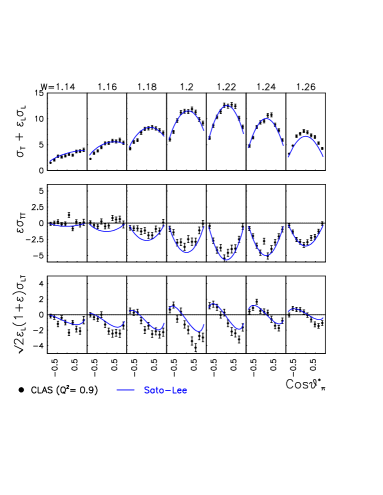
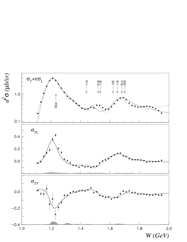
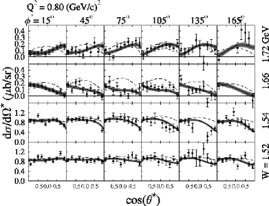
As can be seen in Table 5.1, pion electroproduction data are now very extensive and of high quality. In Figs. 9, 10, and 11, we show some sample data from CLAS at JLab. As an example for a spectrum with high statistics data on $\pi^{\circ}$ electroproduction at a fixed backward angle of $\theta^{cm}_{\pi^{\circ}}=170^{\circ}$ we show in Fig. 12 response functions recently obtained from JLab Hall A ^?.

In Fig. 9 and Fig. 11, the predictions from the SL, MAID, and DMT models are also displayed to illustrate the status of current reaction models. The analyses of these new data in the past few years have led to rather accurate determinations of the $\gamma N\rightarrow\Delta$ transition form factors. We now discuss this advance in more detail.

Figure 9: $p(e,e^{\prime}\pi^{0})$ cross section data from CLAS at JLab are compared with the predictions from the SL Model.

Figure 10: $ep\rightarrow en\pi^{+}$ data from CLAS. Separated response functions $\sigma_{T}+\epsilon\sigma_{L}$, $\sigma_{TT}$, and $\sigma_{LT}$ are shown. The curve represents a fit to the data using the JLab/Yeveran unitary isobar model .

Figure 11: CLAS data on $\sigma_{LT^{\prime}}$ of $p(e,e^{\prime}\pi^{+})n$ reaction in the $\Delta(1232)$ region are compared with predictions from SL(solid), MAID(dashed), and DMT(dashed-dotted) models.

Figure 12: Unpolarized response functions for $p\pi^{\circ}$ at $\theta^{cm}_{\pi^{\circ}}=170^{\circ}$ from JLab Hall A. The solid line corresponds to a fit to the data using the MAID03 implementation. The dashed line corresponds to the SAID solution.

5.1.3 The $\gamma N\rightarrow\Delta(1232)$ transition form factors

With the fairly extensive coverage over angles and energies, the data from JLab have allowed nearly model-independent determinations of $\gamma N\rightarrow\Delta(1232)$ form factors. Theses analyses by the CLAS collaboration are based on the following considerations. At the $\Delta$ peak, the dominant amplitude is $M_{1+}$ and the small $E_{1+}$ and $S_{1+}$ can become accessible through their interference with the dominant $M_{1+}$ amplitude. One thus can start the analysis by using a truncation, in which only terms involving $M_{1+}$ are retained. With the partial-wave decomposition defined by Eqs.(35)-(40), the differential cross section in Eq.(17) can then be written as

$$\frac{d\sigma}{d\Omega^{*}}=\sum_{\ell=0}^{2}A_{\ell}P_{\ell}(cos\theta^{*})+[\sum_{\ell=1}^{2}B_{\ell}P^{\prime}_{\ell}(cos\theta^{*})]cos\phi_{M}+[C_{2}P^{\prime}_{2}(cos\theta^{*})]cos2\phi_{M}$$ (110)

The coefficients of the above equation are related to $|M_{1+}|^{2}$ and its projection onto the other s- and p-wave multipoles $E_{1+}$, $S_{1+}$, $M_{1-}$, $E_{0+}$, $S_{0+}$ :

$$|M_{1+}|^{2} = A_{0}/2,$$ (111)

$$Re(E_{1+}M^{*}_{1+}) = (A_{2}-2C_{2}/3)/8,$$ (112)

$$Re(M_{1-}M^{*}_{1+}) = -[A_{2}+2(A_{0}+C_{2}/3)]/8,$$ (113)

$$Re(E_{0+}M^{*}_{1+}) = A_{1}/2,$$ (114)

$$Re(S_{0+}M^{*}_{1+}) = B_{1},$$ (115)

$$Re(S_{1+}M^{*}_{1+}) = B_{2}/6.$$ (116)

The partial wave coefficents of Eq.(110) are determined by fitting the differential cross sections data such as those displayed in Figs. 9 - 11. From the relations Eqs.(111)-(116), one then obtains the $M_{1+}$, $E_{1+}$ and $S_{1+}$ amplitudes for determining the $\gamma N\rightarrow\Delta$ form factors through Eqs.(99)-(101).

The results from using the above procedure must be corrected for the systematic errors due to the truncation of higher multipoles. This can be accomplished by calculating the effects of higher partial waves using a realistic parametrization of the higher mass resonances and a realistic model for the background amplitudes. For not too large $Q^{2}$ values, this method results in reliable multipoles.

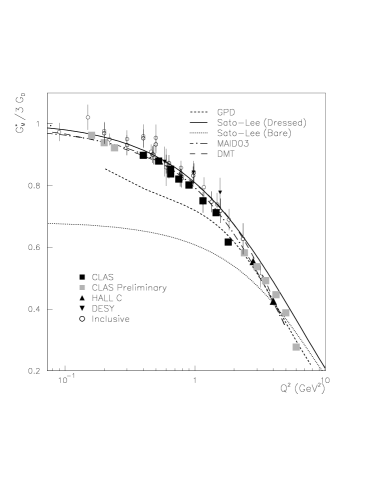
With the above largely model-independent procedure, results for $G^{*}_{M}$ up to $Q^{2}=$ 6 GeV² and the ratios $R_{EM}$ and $R_{SM}$, defined in Eqs.(102) and (103), up to $Q^{2}=4$ GeV² have been obtained at JLab and are compared with various theoretical predictions in Figs. 13 and  14. We now explain how the displayed results from SL, MAID, and DMT models are obtained. Within the MAID model, the $Q^{2}$-dependence of the $\gamma N\rightarrow N^{*}$ transition strengths $\bar{A}^{\alpha}$ of Walker’s parameterization Eq.(64) is determined from fitting the differential cross section data. The resulting multipole amplitudes are then used to extract the $\gamma N\rightarrow\Delta$ form factors by using Eqs.(99)-(101). On the other hand, within the SL and DMT dynamical models, the parameters of the bare quantities $G_{M}(Q^{2})$, $G_{E}(Q^{2})$ and $G_{C}(Q^{2})$, defined by Eq.(93), are adjusted to fit the data. The dressed form factors of the SL model are then predicted by using Eq.(84) to calculate the meson cloud effect. As shown in Ref.^?, at the $\Delta$ mass $W=1.232$ GeV this procedure is equivalent to that based on Eqs.(99)-(101). The parameters of these three models have been determined by using the data up to $Q=4$ GeV². The results at $Q^{2}>4$ GeV² are their predictions.

In Fig. 13, we see that the theoretical predictions of $G^{*}_{M}(Q^{2})$ at $Q^{2}>$ 4 (GeV/c)² from SL , MAID, and DMT models agree well with the new data from Jlab. The prediction by Stoler^?, which is based on a PQCD-motivated model, is also displayed there for comparison. It also agrees well with the data at relatively high $Q^{2}$.

The dotted curve in Fig. 13 is obtained from setting the pion cloud effect, defined by Eq.(84) and illutrated in Fig. 7, to zero within the Sato-Lee model. We see that the pion cloud effect is very large at low $Q^{2}$, but becomes much smaller at high $Q^{2}$. Clearly this $Q^{2}$ dependence plays an important role in getting the agreement with the data up to $Q^{2}$=6 GeV². It will be interesting to see whether the predicted pion cloud effect will agree with the data at even higher $Q^{2}$.

Figure 13: The data of magnetic form factor $G^{*}_{M}$ for the $\gamma N\rightarrow\Delta(1232)$ transition are compared to various models. Results from old single arm electron scattering experiments are labeled “inclusive”. All other results have been obtained from a multipole expansion of exclusive $\pi^{\circ}$ production from protons.

Figure 14: Ratios $R_{EM}$(denoted as $E_{1+}/M_{1+})$ and $R_{SM}$(denoted as $S_{1+}/M_{1+})$ for the $\gamma N\rightarrow\Delta(1232)$ transition. These two ratios are related to the $E^{3/2}_{1+}$, $S^{3/2}_{1+}$, and $M^{3/2}_{1+}$ multipole amplituds of $\gamma^{*}N\rightarrow\pi N$, as defined in Eqs.(102)-(103). Preliminary data from CLAS at low $Q^{2}$ are also included.

Figure 15: The data of $A_{LT}$ from MIT-Bates are compared with the results from Sato-Lee model. The dashed curve is obtained from setting the $G_{C}$ and $G_{E}$ of the $\gamma N\rightarrow\Delta$ form factor to zero.

Figure 16: The imaginary parts ($Im$) of the $E_{1+}^{3/2}$ and $S_{1+}^{3/2}$ calculated from the Sato-Lee model. The dotted curves are obtained from setting the pion cloud effect to zero.

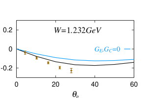
In the upper part of Fig. 14, we see that the preliminary CLAS data for $R_{EM}$ at low $Q^{2}<0.2$ (GeV)^2 ? are in good agreement with the predictions from the SL and DMT models. On the other hand, the new Jlab data for the ratio $R_{SM}$ (lower part of Fig. 14) in the low $Q^{2}<0.2$ GeV² region prefers the prediction from the SL model. The data points at $Q^{2}=0.127$ GeV² from MAMI and Bates have a larger magnitude for $R_{SM}$. These data points were used by DMT in fixing their parameterization for $G_{C}(Q^{2})$. It should be noted that the points from MAMI and Bates are not the result of an independent multipole fit, but are from data sets with more limited angle coverage fitted to the MAID parametrization. One of the data sets from MIT-Bates is shown in Fig. 15. Clearly, only very limited angles are covered. Nevertheless, these data are very useful in revealing the non-zero values of the $G_{E}$ and $G_{C}$ form factors within the dynamical model, as illustrated in the difference between the solid and dotted curves.

We now note that the ratios $R_{EM}$ and $R_{SM}$ calculated from the dynamical models are very much related to the predicted pion cloud effects. These are illustrated in Fig. 16 from the SL model. We see that the pion cloud effect can strongly enhence the the $E^{3/2}_{1+}$ and $S^{3/2}_{1+}$ amplitudes of $\gamma^{*}N\rightarrow\pi N$ at low $Q^{2}$. As defined in Eqs.(99)-(101), these two amplitudes are related to the $G_{E}(Q^{2})$ and $G_{C}(Q^{2})$ of $\gamma N\rightarrow\Delta$ transition. The non-trivial pion cloud effects shown in Fig. 16 are clearly verified by the JLab data, as seen in Fig. 14.

To further improve the determination of the $\gamma N\rightarrow\Delta$ form factors, data of polarization observables must be included in the theoretical analyses. Measurements using polarized electron beam and/or a longitudinally polarized hydrogen target ^? have yielded data of double spin beam-target asymmetry $A_{et}$ and target asymmetry $A_{t}$. Samples of asymmetry data from CLAS are shown in Fig. 17.

Figure 17: $A_{et}$ and $A_{t}$ from JLab at W=1.225 GeV, $Q^{2}=0.46GeV^{2}$ are compared with the predictions from SL, MAID, and DMT models. The left panel is integrated in a range $\phi=(144^{\circ},160^{\circ})$. The right panel is integrated in a range $\cos{\theta^{*}}=(-0.6,-0.8)$.

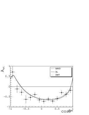
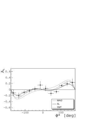
The double polarization asymmetry $A_{et}$ is largely given by the well determined $M_{1+}$ multipole and is well described by all models. However, significant differences can be seen in the $A_{t}$ asymmetry which is sensitive to interferences between the non-resonant and resonant amplitudes. The discrepancy in the model descriptions can be attributed to their different treatments of the non-resonant amplitudes, as discussed in section 4.

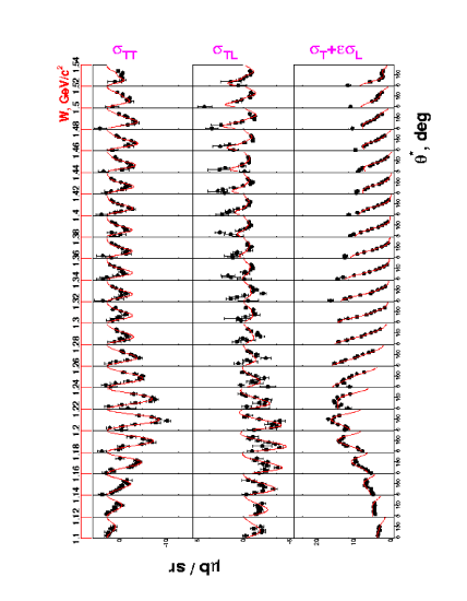
Extensive pion electroproduction data in the second and third resonance regions have also been obtained using CLAS. Some typical results are shown in Figs. 18. Here we see that the displayed theoretical predictions do not agree well with the data at $W>1.4$ GeV. This is not surprising since the parameters of these single-channel models are fixed by mainly fitting the data at $W<1.4$ GeV. Recently, fits to these higher $W$ data have been achieved by using a single-channel K-matrix model and fixed-t dispersion relations. In these analyses $p\pi^{\circ}$ and $n\pi^{+}$ data are fitted simultaneously using unpolarized cross section data as well as beam spin response function results. It has been found that these very different approaches give consistent results, e.g. in the analyses of Aznauryan et al. ^?. It indicates that the model-dependence may be relatively small. Nevertheless, the extracted resonance parameters must be taken with caution before a rigorous investigation of the coupled-channel effect has been carried out. Progress in this direction is being made ^?. The results of these fits are discussed in section 5.3.

Figure 18: The data of $\sigma_{LT^{\prime}}$ for $\gamma^{*}p\rightarrow p\pi^{\circ}$ in the $2^{nd}$ resonance region are compared with MAID (dashed) and the DMT (dashed-dotted) predictions.

5.2 Photoproduction and electroproduction of $\eta$ mesons.

In contrast to the pion with isospin I = 1, the eta is an isoscalar meson with no charged partners. As such it can only couple with nucleons to form I = 1/2 resonances. This makes the production of $\eta$’s from nucleon targets an ideal tool to separate isospin $1\over 2$ $N^{*}$ resonances from isospin $3\over 2$ $\Delta^{*}$ resonances. The total photoproduction cross section, shown in Fig. 19, exhibits a rapid rise just above threshold, indicative of a strong s-wave contribution near threshold. This behavior is known to be due to the first negative parity nucleon resonance, the $S_{11}(1535)N_{1/2^{-}}$, which couples with approximately 55% to the $N\eta$ channel ^?. The nearby $D_{13}(1520)$ has a branching ratio of much less than 1% to this channel. The next higher mass nucleon resonance with a significant $N\eta$ coupling is the $P_{11}(1710)$, nearly 200 MeV/c² higher in mass. This fact makes the production of $\eta$’s from nucleon targets the reaction of choice for detailed studies of the electromagnetic transition from the ground state to the $S_{11}(1535)$. The $N\eta$ channel effectively isolates this state from other nearby resonances, similar to the $\Delta(1232)$ which is well separated from higher mass resonances in the $p\pi^{\circ}$ channel. In distinction to the $\Delta(1232)$, whose electromagnetic transition form fcators drop rapidly with increasing photon virtuality $Q^{2}$, the $S_{11}(1535)$ remains a prominent resonance even at the highest $Q^{2}$ that are currently accessible.

Figure 19: Total cross section for $\eta$ photoproduction from protons. Data from MAMI (open circles), GRAAL (full circles), and CLAS (open squares) are shown. The curves are the fits explained in section 5.2.4.

In the following subsections we discuss the status of the electromagnetic production of $\eta$’s from nucleons, and analyses to extract the photocoupling helicity amplitudes for the $\gamma N\rightarrow S_{11}(1535)$ transition, and their $Q^{2}$ evolution. We finally compare the results with model predictions. Table 5.2 gives an overview of the kinematics covered in recent $\eta$ production measurements ^{?,?,?,?,?,?,?,?,?,?}.

Table 4. Summary of $\eta$ production data

Table 4. Summary of $\eta$ production data

Reaction Observable W range $Q^{2}$ range Lab. (GeV) (GeV²) $\gamma p\rightarrow p\eta$ $d\sigma/d\Omega$ $<2.0$ JLab-CLAS $d\sigma/d\Omega$ $<1.7$ GRAAL $d\sigma/d\Omega$ $<2.3$ ELSA-CB $d\sigma/d\Omega$ $<1.53$ MAMI-TAPS $\gamma(n/p)\rightarrow(n/p)\eta$ $d\sigma_{n}/d\sigma_{p}$ $<2.3$ GRAAL $\vec{\gamma}p\rightarrow p\eta$ $\Sigma$ $<2.3$ GRAAL $\gamma\vec{p}\rightarrow p\eta$ $T$ $<2.3$ ELSA $\vec{\gamma}\vec{p}\rightarrow p\eta$ $E$ $<1.53$ MAMI-A2 $ep\rightarrow ep\eta$ $\sigma_{LT}$, $\sigma_{TT}$, $\sigma_{T}+\epsilon\sigma_{L}$ $<2.2$ 2.8 - 4.0 JLab-Hall-C $\sigma_{LT}$, $\sigma_{TT}$, $\sigma_{T}+\epsilon\sigma_{L}$ $<2.2$ 0.3 - 4.0 JLab-CLAS

5.2.1 $\eta$ photoproduction from protons

With the new measurements in recent years, the data base for $\eta$ photoproduction reaction has been improved tremendously. The differential cross section data now cover the $p\eta$ mass range up to W = 2.3 GeV, and are available for most of the angular range in the hadronic center-of-mass system. Some of these data are shown Figure 20. The data from all three experiments agree well.

Figure 20: Differential cross section for $\gamma p\rightarrow p\eta$ from TAPS, GRAAL, and CLAS are shown for photon energies near threshold to 1.875 GeV. The curves are the fits explained in section 5.2.4. The solid (dotted) line represents the UIM (DR) analysis.

In the mass region of the $S_{11}(1535)$ resonance the angular distributions are nearly flat, indicating dominant s-wave components with only slight indications of higher partial wave contributions. In the mass region above 1.750 GeV, the angular distributions become increasingly forward-peaked, indicating significant non-resonant behavior presumably due to t-channel processes.

GRAAL has measured the beam asymmetries using laser light backscattered from the 6 GeV electrons to generate high-energy linearly polarized photons. The beam asymmetry $\Sigma_{\gamma}$ is defined as

$$\Sigma_{\gamma}={1\over P_{\gamma}}{{{d\sigma\over d\Omega}(\phi=0^{\circ})-{d\sigma\over d\Omega}(\phi=90^{\circ})}\over{{d\sigma\over d\Omega}(\phi=0^{\circ})+{d\sigma\over d\Omega}(\phi=90^{\circ})}}$$ (117)

where $P_{\gamma}$ is the photon polarization, $\phi$ is the azimuthal angle between the plane defined by the linear photon polarization and the hadronic plane defined by the photon beam and the $p\eta$ final state. The measured beam asymmetries are shown in Fig. 21. Just above $\eta$ threshold and at the resonance position $\Sigma_{\gamma}$ shows a symmetric angular distribution, approximately following a $\sin^{2}\theta^{*}$ behavior, while at higher energies the asymmetry is more forward peaked. The $\sin^{2}\theta^{*}_{\eta}$ behavior near the resonance pole at the lower energies is prominent in the data, and is also reflected in the model descriptions included in Fig. 21.

Asymmetries have also been measured with a transversely polarized proton target at ELSA. The target asymmetry $T$ is given by:

$$T={1\over P_{T}}{{{d\sigma\over d\Omega}(\uparrow)-{d\sigma\over d\Omega}(\downarrow)}\over{{d\sigma\over d\Omega}(\uparrow)+{d\sigma\over d\Omega}(\downarrow)}}.$$ (118)

The arrows indicate the direction of the proton polarization relative to the hadronic plane. Results are shown in the right panel in Fig. 21.

Figure 21: The fits to the $\gamma p\rightarrow p\eta$ data using the Unitary Isobar Model (solid curves) and Dispersion Relation (short dashed curves)approaches. Left panel: Beam asymmetry measured at GRAAL. The dotted curve in the 1050 MeV panel shows the fit without the $F_{15}(1680)$ resonance. Right panel: Target asymmetry measured at ELSA.

5.2.2 $\gamma p\rightarrow S_{11}(1535)$ parameters extracted from gobal fit to $\eta$ photoproduction

The $S_{11}(1535)$ has long been known as a strong nucleon resonance with a large branching ratio to the $N\eta$ and $N\pi$ channels. However, there have been assertions that the strong enhancement near this mass is not due to the excitation of a resonance ^?. One model implies that the state is dominantly a dynamically generated $\Sigma\bar{K}$ resonance ^?. On the other hand, recent Lattice QCD calculations ^?,? show that there is a strong 3-quark state at this mass with the spin-parity $J^{P}={1\over 2}^{-}$, indicating that the $S_{11}(1535)$ is indeed an excited state of the nucleon.

The photocoupling amplitudes and their $Q^{2}$ dependence are powerful tools in determining the internal resonance structure and will help solve this controversy. For the purpose of this article we consider the $S_{11}(1535)$ as a baryon resonance with well defined quantum numbers. In the following we discuss results obtained in a global analysis of all observables in $\eta$ photoproduction with the goal to extract the photocouplings amplitudes for resonances coupling to the $p\eta$ channel, especially the $S_{11}(1535)$.

A number of analyses have been performed on the $p\eta$ photoproduction channel ^?,?,?. Here, we describe the recent global analysis by Aznauryan^? as it allows to also assess the model-dependence of the results. Differential cross sections ^?,? were included as well as polarized beam asymmetries ^?, and polarized target asymmetries ^?. All established $N^{*}$ resonances above the $N\eta$ threshold were included, i.e. $S_{11}(1535)$, $D_{13}(1520)$, $S_{11}(1650)$, $D_{15}(1675)$, $F_{15}(1680)$, $D_{13}(1700)$, $P_{11}(1710)$, $P_{13}(1720)$. The cross section data are fitted for photon energies up to 2 GeV, corresponding to invariant masses in the range W = 1.49 - 2.15 GeV, i.e. covering the entire resonance region. The polarization data cover only the range up to W = 1.7 GeV. Figure 20 and Fig. 21 show samples of the fit to the cross sections and asymmetry data. The Unitary Isobar Model (UIM) and Dispersion-relations (DR) approaches give consistent results for the $S_{11}(1535)$, $D_{13}(1520)$, and $F_{15}(1680)$ resonances. The first result is the confirmation of a large photocoupling amplitude for the $S_{11}(1535)$ which is determined with good precision. The results are summarized in table 5.2.2.

Table 5. $S_{11}(1535)$ photocoupling from gobal fit in units ($10^{-3}~{}GeV^{-1/2}$).

Table 5. $S_{11}(1535)$ photocoupling from gobal fit in units ($10^{-3}~{}GeV^{-1/2}$).

Resonance Mass (MeV) $\Gamma$ (MeV) $A^{p}_{1/2}$ Model $S_{11}(1535)$ 1527 142 96 Isobar model 1542 195 119 Dispersion relations 1520-1555 100-200 60 - 120 PDG estimate

They are compared with the range given by the PDG ^?. The new results are within the upper part of the range given by the PDG. The lower range in the PDG value comes from an analysis of pion production data by the George Washington University (GWU) group^?. We note here that the results from the global fits are also in good agreement with a combined analysis of $\pi$ and $\eta$ electroproduction data. We will discuss this in section 5.3.

From the fit to the differential cross sections one can then also extract the total photo absorption cross section for $\eta$ production. The fit results are compared with the experimental data in Fig. 19. All three experiments agree well in the region where the $S_{11}(1535)$ resonance dominates, while there is a discrepancy near 1100 MeV photon energy. Since the angular distributions agree well, this discrepancy must be entirely due to different models used for the extrapolation into the unmeasured angular regions. This emphasizes the importance of measureing complete angular distributions which are now available ^?.

The global analysis incorporates also the beam asymmetry in the fit. To illustrate the sensitivity of $\Sigma$ to contributions from the $D_{13}(1520)$ we express $\Sigma_{\gamma}$ in the approximation that only S-waves, P-waves, and D-waves with spin $J\leq{3\over 2}$ contribute as ^?:

$$\Sigma_{\gamma}\approx{3\sin^{2}\theta Re[E^{*}_{0+}(E_{2-}+M_{2-})]\over|E_{0+}|^{2}}$$ (119)

Table 6. Summary of $\eta$ photoproduction gobal fit results. The uncertainty in $\beta_{\eta N}$ reflects the model dependence in using the unitary isobar model and dispersion relation approach.

Table 6. Summary of $\eta$ photoproduction gobal fit results. The uncertainty in $\beta_{\eta N}$ reflects the model dependence in using the unitary isobar model and dispersion relation approach.

Resonance Mass(MeV) $\Gamma(MeV)$ $\beta_{\eta N}$(%) $\beta_{\pi N}$(%) $D_{13}(1520)$ 1520 120 0.05 $\pm$ 0.02 50 - 60 $F_{15}(1680)$ 1675 130 0.15 $\pm$ 0.03 60 - 70

This expression can be fitted to the measured beam asymmetry $\Sigma_{\gamma}$. Using $E^{*}_{0+}$ from fits to the cross section data, the multipoles $E^{\eta}_{2-},~{}M^{\eta}_{2-}$ for the $D_{13}(1520)$ can then be determined. Since the corresponding pion multipoles $E^{\pi}_{2-},~{}M^{\pi}_{2-}$ are known with high precision from pion production, the branching ratio $\beta_{\eta N}$ can be extracted. The analysis also allows to extract the $N\eta$ branching ratio for the $F_{15}(1680)$ by analyzing the forward-backward asymmetry in $\Sigma_{\gamma}$ seen in Fig. 21 at $E_{\gamma}\approx 1$ GeV. The dotted curve in the figure for 1050 MeV (left panel) shows the fit when the small $F_{15}(1680)$ amplitudes are turned off. Clearly, the ( interference effects strongly enhance this contribution. The results for the $D_{13}(1520)$ and $F_{15}(1680)$ are summarized in table 5.2.2. Both results represent significantly improved values for the branching ratios.

Figure 22: Samples of differential cross section for $\gamma^{*}p\rightarrow p\eta$ from CLAS at fixed $Q^{2}=0.8$ GeV² and different W and $\phi$ values. The shaded bands indicate the fit results using 9 Legendre polynomials, as explained in section 5.2.5. The dashed curve represents the predictions of $\eta$MAID.

5.2.3 Eta electroproduction

Eta electroproduction experiments have focussed on the $Q^{2}$ evolution of the $S_{11}(1535)$ transverse photocouplings amplitude $A_{1/2}(Q^{2})$. Experiments at DESY ^?,? and Bonn ^?,? found a very slow falloff with $Q^{2}$. Recent experiments at Jefferson Lab ^?,?,? have studied this behavior in detail with high statistics, and also extended the kinematics range. Figure 22 shows samples of differential cross sections measured with CLAS ^?. Even at the peak of the $S_{11}(1535)$ resonance the angular distributions are not completely flat indicating that higher partial waves are present in addition to the dominant S-wave.

Figure 23: Left panel: Total cross section for $\gamma^{*}p\rightarrow p\eta$ vs W, at various photon virtualities $Q^{2}$. The right panel shows partial wave fit parameters vs W compared to predictions of $\eta$MAID. All data are from CLAS.

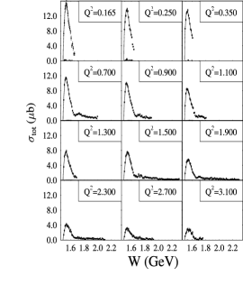
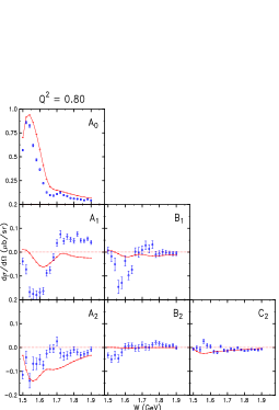
Figure 23 shows samples of total cross sections at fixed $Q^{2}$. In contrast to the $\Delta(1232)$ which rapidly drops with $Q^{2}$, the $S_{11}(1535)$ remains prominent even at the highest $Q^{2}$.

Most of the published results on the $Q^{2}$ dependence of the $S_{11}(1535)$ transition amplitude have been obtained in single resonance fits. This has been justified with the dominant contributions of the $S_{11}(1535)$ to the $\gamma^{*}p\rightarrow p\eta$ cross section. It is, however, not a fully satisfactory solution, as higher mass states that couple to $N\eta$ may also contribute in the lower mass region. The results have to be taken with caution. The differential cross sections are fitted to the expression Eq.(17). The dependence on the $\eta$ scattering angle ($\theta^{*}_{\eta}$) can be examined by expanding each component of the differential cross section in terms of Legendre polynomials:

$${d\sigma_{T}\over{d\Omega}^{*}_{\eta}}+\epsilon{d\sigma_{L}\over{d\Omega}^{*}_{\eta}} = {\sum_{\ell=0}^{\infty}}A_{\ell}P_{\ell}(\cos\theta^{*}_{\eta})$$ (120)

$$\sqrt{2\epsilon(\epsilon+1)}{d\sigma_{LT}\over{d\Omega}^{*}_{\eta}} = {\sum_{\ell=1}^{\infty}}B_{\ell}P_{\ell}^{\prime}(\cos\theta^{*}_{\eta})$$ (121)

$$\epsilon{d\sigma_{TT}\over{d\Omega}^{*}_{\eta}} = {\sum_{\ell=2}^{\infty}}C_{\ell}P_{\ell}^{\prime\prime}(\cos\theta^{*}_{\eta})$$ (122)

If the expansion is limited to $\ell=2$, only the coefficients $A_{0},~{}A_{1},~{}A_{2},~{}B_{1},~{}B_{2}$ and $C_{2}$ are retained. Results from the fit at fixed $Q^{2}$ are shown in the right panel of Fig. 23. Strong variations of $A_{1}$ and $B_{1}$ are seen in the W range from 1.6 to 1.7 GeV, indicating large interference effects involving s- and p-waves. Possible p-wave candidates are the $P_{11}(1710)$ and $P_{13}(1720)$ states. $A_{0}$ is mostly due to the $S_{11}(1535)$ resonance, and is the by far largest amplitude. The longitudinal and transverse response functions cannot be separated in this analysis. In earlier experiments ^?,? the longitudinal and transverse cross sections were separately determined at some fixed $Q^{2}$ values, showing that $A_{0}$ is dominated by the transverse amplitude $A_{1/2}^{2}$ in the $Q^{2}$ range of this study. The combined analysis of $\pi$ and $\eta$ electroproduction data, to be discussed in the next section, also finds small longitudinal contribution to $A_{0}$. Assuming $\sigma_{L}=0$, $|A_{1/2}|$ can be computed from $A_{0}$. Figure 24 shows a compilation of results for the $\gamma p\rightarrow S_{11}(1535)$ photocouplings helicity amplitude $A_{1/2}(Q^{2})$. The slow falloff with $Q^{2}$ confirms the unusually hard transition form factor that persists to the highest measured values of $Q^{2}$. The solid and dotted curves are the prediction of Close and Li ^?, and of Giannini, Santopinto and Vassallo ^?.

Figure 24: $Q^{2}$ evolution of the $\gamma p\rightarrow S_{11}(1535)$ photocouplings amplitude $A_{1/2}$. The full symbols are the most recent CLAS results. The open diamonds are the JLab data from Hall C, and the open circles are from previous experiments. The solid curve is from Ref.(177), and the dotted curve is from Ref.(175).

It should be noted that the absolute normalization of the data displayed in Fig.24 is uncertain to the extent that the branching ratio $\beta_{N\eta}(S_{11})=0.55$ and a total widths of 150 MeV have been used in extracting $A_{1/2}$. The Review of Particle Properties 2002 allows a large range of 0.30 - 0.55 for the branching ratio. However, the recent analysis of Armstrong et al. ^?, gives a value of $\beta_{N\eta}(S_{11})\approx 0.55$. The use of this value is consistent with the values $\beta_{N\eta}(S_{11})=0.55$ and $\beta_{N\pi}(S_{11})=0.4$ used in the combined analysis of $\pi$ and $\eta$ electroproduction which is the subject of next section.

5.3 Combined analysis of $\pi$ and $\eta$ electroproduction data

The large amount of data taken by the CLAS detector allows simultaneous measurements of cross sections and polarization observables for several channels, e.g. $p\pi^{\circ},~{}n\pi^{+},~{}p\eta$. Also, the large acceptance provides complete angular distributions, including the full azimuthal dependence. Use of a highly polarized electron beam provides data on the helicity-dependent response function $\sigma_{LT^{\prime}}$ covering the full angle range. Results of a MAID and DMT analysis of the channel $p\pi^{\circ}$ have recently been reported ^?. Combined analyses of these data in a multi-channel global fit provides much more stringent constraints on resonance parameters than single-channel analyses can. The full set of data taken with a hydrogen target have been analyzed within the unitary isobar model ^? and the dispersion relation approach ^? described in section 4. The data on $\sigma_{LT^{\prime}}$ are especially sensitive to small resonance contributions in a large non-resonant background. The sensitivity is the result of the interference term that mixes real and imaginary amplitudes

$$\sigma_{LT^{\prime}}\sim Im(L)\cdot Re(T)+Im(T)\cdot Re(L)~{},$$ (123)

where L and T represent the longitudinal and transverse amplitudes, respectively. Figure  25 shows the the sensivity of $\sigma_{LT^{\prime}}$ to the $P_{11}(1440)$ multipoles $M_{1-}$ and $S_{1-}$. Both channels show sensitivity to changes in the multipoles, however, the effect is much larger in the $n\pi^{+}$ channel. This is due to a combination of two factors, the stronger coupling of $I=1/2$ nucleon states to the $n\pi^{+}$ channel, and the larger background terms contributing to this channel. Using pion and eta production to study the same resonances, e.g. the $S_{11}(1535)$ allows tests of possible flavor-dependence of the results which could be significant if rescattering effects, such as present in the $\Delta(1232)$ region, play an important role also for higher mass states. The use of two conceptually very different approaches also allow to estimate the model-dependence of the resulting amplitudes.

Figure 25: Sensitivity of CLAS data of $\sigma_{LT^{\prime}}$ to changes in multipoles $M^{1/2}_{1-}$ (dashed) and $S_{1-}^{1/2}$ (dotted) for $n\pi^{+}$ channel (left) and $p\pi^{\circ}$ channel (right). Solid line shows best fit using the Unitary Isobar Model. The -0.5 in the legend refers to shifting the Breit-Wigner amplitude by -0.5 $\mu b^{1/2}$.

The results for the $P_{11}(1440)$ are shown in Fig. 26. For the first time a consistent trend is emerging: The magnitude of $A_{1/2}(Q^{2})$ drops rapidly for $Q^{2}>0$, with a sign change near $Q^{2}=0.5$ GeV². There is also a strong longitudinal coupling. Bold, solid, dashed and dot-dashed lines are from various calculations^?,?,?,?. Nonrelativistic quark models^?,? predict large negative $A_{1/2}(Q^{2})$ in the entire $Q^{2}$ range, and do not describe the data. The hybrid model^? describes the fast drop of $|A_{1/2}|$ qualitatively, but has no sign change, and predicts $S_{1/2}(Q^{2})=0$, while the data show a sizeable $S_{1/2}$ amplitude. The relativistic models of Capstick and Keister ^? and of Cardarelli and Simula ^? predict the sign change for $A_{1/2}(Q^{2})$ but show a much faster rise than is observed. The magnitudes and trends of both amplitudes are well described by a model that describes the $P_{11}(1440)$ with a small quark core and a $q\bar{q}$ cloud ^?. In this model, the low $Q^{2}$ behavior is entirely due to the $q\bar{q}$ contribution while the $qqq$ core defines the high $Q^{2}$ behavior.

Figure 26: Results for the $P_{11}(1440)$ amplitudes $A^{p}_{1/2}$ and $S^{p}_{1/2}$. CLAS points include model error. The Hall A point shows MAID03 fit model error. The curves are described in the text.

Figure 27: $Q^{2}$ evolution of the $S_{11}(1535)$ photocoupling amplitudes $A_{1/2}(Q^{2})$ (left), and $S_{1/2}(Q^{2})$ (right). Cross section data from $p\eta$, $p\pi^{\circ}$, and $n\pi^{+}$ have been used, as well as polarized beam response function $\sigma^{\pi^{+}}_{LT^{\prime}}$ and $\sigma^{\pi^{\circ}}_{LT^{\prime}}$. The shaded band indicates the uncertainties seen in previous analysis using $p\eta$ cross sections data. Solid and dotted lines are from quark model calculations described in the text.

Figure 28: $Q^{2}$ evolution of the $D_{13}(1520)$ photocoupling amplitudes $A_{1/2}$, $A_{3/2}$, and $S_{1/2}$. Cross section data from $p\pi^{\circ}$, and $n\pi^{+}$ have been used, as well as polarized beam response function $\sigma^{\pi^{+}}_{LT^{\prime}}$ and $\sigma^{\pi^{\circ}}_{LT^{\prime}}$. The shaded bands indicate the uncertainties seen in previous analysis using mostly $p\pi^{\circ}$ cross section data. The theoretical curves are explained in the text.

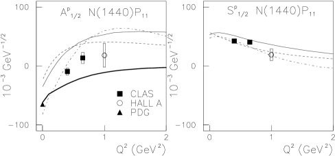
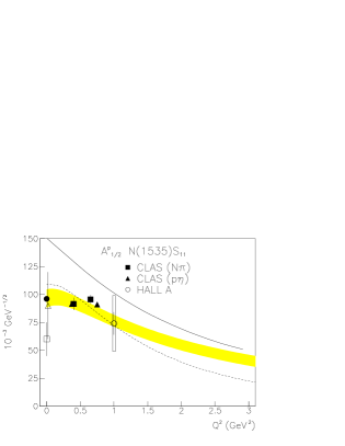
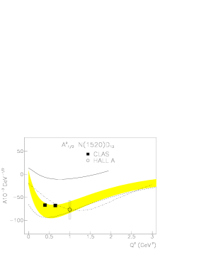
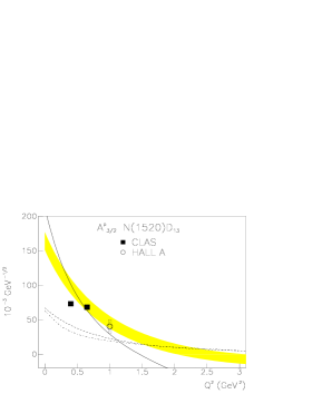
The results for the $S_{11}(1535)$ are depicted in Fig. 27. They show consistent results for $A_{1/2}$ in the $p\eta$ and the $N\pi$ channels for the Unitary Isobar Model (UIM) and Dispersion-Relation (DR) analyses. Also, for the first time, stable results for the longitudinal coupling $S_{1/2}$ have been obtained. The solid and dotted curves in Fig.27 represent quark model calculations using a harmonic oscillator potential ^? and a hypercentral potential ^?, respectively.

The results of the global fit for $A_{1/2},~{}A_{3/2}$ and $S_{1/2}$ for the $D_{13}(1520)$ are shown in Fig. 28. Both the UIM and DR analyses give consistent results. To summarize, the inclusion of polarization observables in addition to the differential cross section into a global analysis results in a less model-dependent description of $\pi$ and $\eta$ photoproduction and electroproduction processes in the resonance region. There are several noteworthy results: First, consistent results are obtained for the mass of the $S_{11}(1535)$ for the $\eta$ and $\pi$ channel, both for photo- and electroproduction. The mass is in the range $M(S_{11})=1531\pm 5$ MeV. Second, the discrepancy between $\eta$ and $\pi$ photoproduction results for $A_{1/2}$ amplitude seems to have been resolved. The analysis of electroproduction data gives also good agreement for the $p\eta$ and $N\pi$ channels and in both UIM and DR approaches. Third, the $Q^{2}$ evolution of the $A_{1/2}$ and $S_{1/2}$ amplitudes for the $P_{11}(1440)$ are consistent with the predictions of a meson cloud model. This is in line with what has been found earlier for the $N\Delta(1232)$ transition, that meson cloud effects can be sizeable for some of the resonance transitions.

5.3.1 Analysis of Resonance Transitions in the Single Quark Transition Model

Properties of nucleon resonances such as mass, spin-parity, and flavor fit well into the representation of the $SU(6)\otimes O(3)$ symmetry group, which describes the spin-flavor and orbital wave functions of the 3-quark system. This symmetry group leads to supermultiplets of baryon states with the same orbital angular momentum $\vec{L}$ of the 3-quark system, and degenerate energy levels. Within a supermultiplet the quark spins are aligned to form a total quark spin $\vec{s}$, with $s={1\over 2}$, $3\over 2$, which combines with the orbital angular momentum $L$ to form the total angular momentum $\vec{J}=\vec{L}+\vec{s}$. A large number of explicit dynamical quark models have been developed to describe the electromagnetic transitions between the nucleon ground state and its excited states ^?,?,?,?. Measurement of resonance transitions and the dependence on the distance scales, given by the virtuality of $Q^{2}$ of the photon, provides information on the nucleon wave function. In order to compute the transition, assumptions on the 3-quark potential and the quark-quark interactions have to be made. These are then tested by predicting photocoupling helicity amplitudes which can then be confronted with experimental data.

Figure 29: Single quark transition amplitudes A, B, C as functions of $Q^{2}$. The amplitudes have been extracted from the recent JLab, MAMI, and GRAAL data on the $S_{11}(1535)$ and world data on $D_{13}(1520)$ photocoupling amplitudes. The shaded band is a parameterization of the data from Ref. 178.

Table 7: Helicity amplitudes for the electromagnetic transition from the ground state $[56,0^{+}]$ to the $[70,1^{-}]$ multiplet as a function of the SQTM amplitudes. $\theta$ is the mixing angle relating two $J^{P}={1\over 2}^{-}$ states with $s_{3q}={3\over 2}$ and $s_{3q}={1\over 2}$. There is also a small mixing angle for the two ${3\over 2}^{-}$ states resulting in the physical states $D_{13}(1520)$ and $D_{13}(1700)$. We have not included the latter mixing angle in the table. Note that the excitation of the $D_{13}(1700)$ from a proton target is only possible because of $SU(6)$ symmetry breaking leading to the mixing with the lower mass $D_{13}(1520)$.

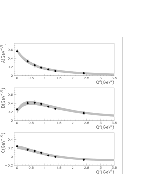
State Proton target Neutron target $S_{11}(1535)$ $A^{+}_{1/2}$ =  ${1\over 6}(A+B-C)\cos\theta$ $A^{\circ}_{1/2}=-{1\over 6}(A+{1\over 6}B-{1\over 3}C)$ $D_{13}(1520)$ $A^{+}_{1/2}=~{}{1\over 6\sqrt{2}}(A-2B-C)$ $A^{\circ}_{1/2}=-{1\over 18\sqrt{2}}(3A-2B-C)$ $A^{+}_{3/2}=~{}{1\over 2\sqrt{6}}(A+C)$ $A^{\circ}_{3/2}=~{}~{}{1\over 6\sqrt{6}}(3A-C)$ $S_{11}(1650)$ $A^{+}_{1/2}=~{}{1\over 6}(A+B-C)\sin\theta$ $A^{\circ}_{1/2}=~{}~{}{1\over 18}(B-C)$ $D_{13}(1700)$ $A^{+}_{1/2}=~{}0$ $A^{\circ}_{1/2}=~{}~{}{1\over 18\sqrt{5}}(B-4C)$ $A^{+}_{3/2}=~{}0$ $A^{\circ}_{3/2}=~{}~{}{1\over 6\sqrt{15}}(3B-2C)$ $D_{15}(1675)$ $A^{+}_{1/2}=~{}0$ $A^{\circ}_{1/2}=-{1\over 6\sqrt{5}}(B+C)$ $A^{+}_{3/2}=~{}0$ $A^{\circ}_{3/2}=-{1\over 6}\sqrt{2\over 5}(B+C)$ $D_{33}(1700)$ $A^{+}_{1/2}=~{}{1\over 6\sqrt{2}}(A-2B-C)$ same $A^{+}_{3/2}=~{}{1\over 2\sqrt{6}}(A+C)$ same $S_{31}(1620)$ $A^{+}_{1/2}=~{}{1\over 18}(3A-B+C)$ same

Algebraic relations have been derived for resonance transitions assuming the transition only affects a single quark in the nucleon. The parameters in these algebraic equations can be determined from the experimental analysis^?. Based on the symmetry properties of the Single Quark Transition Model (SQTM), predictions for a large number of resonances belonging to the same $SU(6)\otimes O(3)$supermultiplet can be made. The fundamentals of the SQTM are described in references ^?,?, where the symmetry properties have been discussed for the transitions from the ground state nucleon $[56,0^{+}]$ to the $[70,1^{-}]$ and the $[56,2^{+}]$ supermultiplets. The $[70,1^{-}]$ contains states which are prominent in electromagnetic excitations, and it is the only supermultiplet for which sufficient data on resonance couplings of two states are available to extract the SQTM amplitudes and test predictions for other states. The coupling of the electromagnetic current is considered for the transverse photon component, and the quarks in the nucleon are assumed to interact freely with the photon. In such a model the quark transverse current can be written in general as a sum of four terms ^?,?,?:

$$J^{+}={AL^{+}+B\sigma^{+}L_{z}+C\sigma_{z}L^{+}+D\sigma^{-}L^{+}L^{+}}~{},\\$$ (124)

where $\sigma$ is the quark Pauli spin operator, and the terms with $A$, $B$, $C$, $D$ in front operate on the quark spatial wave function changing the component of orbital angular momentum along the direction of the momentum transfer (z- axis). The $A$ term corresponds to a quark orbit flip with $\Delta L_{z}=+1$, term $B$ to a quark spin flip with $\Delta L_{z}=0$, the $C$ and $D$ terms correspond to simultaneous quark orbit and quark spin flip with orbital angular momentum flips of $\Delta{L_{z}}=+1$ and $\Delta{L_{z}}=+2$, respectively. For the transition from the $[56,0^{+}]$ to the $[70,1^{-}]$ supermultiplet with $L=1$, only $A$, $B$, and $C$ are allowed. The relationship between the A, B, C amplitudes and the usual helicity photocoupling amplitudes $A_{1/2}$ and $A_{3/2}$ is listed in table 7.

Figure 30: Single quark model transition prediction for the $[70,1^{-}]$ multiplet. The SQTM predictions are shown by the shaded band in comparison with the experimental data. At $Q^{2}=0$ the full circle is the Particle Data Group estimate. For $Q^{2}>0$, measurements from JLab, Bonn, DESY, and NINA in $\eta$ and $\pi$ electroproduction are shown. For the $S_{11}(1535)$, the results of an analysis of the world data in $\eta$-electroproduction presented in Ref. ^? are also included. The superscript ^o refers to neutron states.

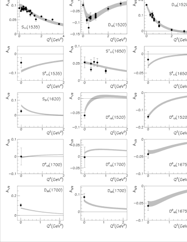
Using the extracted photocoupling amplitudes from the $S_{11}(1535)$ and the $D_{13}(1520)$, the A, B, C amplitudes for the $\gamma+[56,0^{+}]\rightarrow[70,1^{-}]$ have been extracted ^?. The results are shown in Fig. 29. Knowledge of the 3 amplitudes and of two mixing angles for the transition to the $[70,1^{-}]$ allows predictions for 16 amplitudes of states belonging to the same supermultiplet. If they can be confirmed for some of the amplitudes, one then has a measure of the degree to which electromagnetic transitions of nucleon resonance are dominated by single quark transitions at the photon point ($Q^{2}=0)$ and, using electroproduction data, examine if and how this is changing as a function of the distance scale at increasing photon virtuality. The SQTM predictions for the proton and neutron amplitudes are shown in Fig. 30. There is remarkable agreement between the predictions and the data at the photon point. For electroproduction, there is good agreement where consistent data sets are available, i.e. for the $S_{11}(1650)$. Much improved electroproduction data are needed for more definite conclusions. Most of the states belonging to the $[70,1^{-}]$ supermultiplet with masses near 1700 MeV couple strongly to $N\pi\pi$ channels. Studies of these channels require use of large acceptance detectors and new, sophisticated analysis techniques. Progress made in these areas will be discussed in the next section. There are similar relations for the transition from the nucleon ground state to the members of the $[56,2^{+}]$ supermultiplet. In this case four SQTM amplitudes can contribute. Unfortunately, the only state for which the two transverse photocoupling amplitudes have been measured in electroproduction is the $F_{15}(1680)$. This is insufficient to extract the four SQTM amplitudes.

5.4 Two-pion production.

Two-pion channels dominante the electromagnetic meson production cross sections in the second and third resonance regions where we hope to resolve the missing resonance problem^? and ultimately determine what basic symmetry group^? is underlying the baryon spectrum. Thus, a detailed understanding of two-pion production is very important in the $N^{*}$ study, and has been pursued very actively in recent years. Very extensive two-pion production data have now been accumulated at JLab, MAMI and ELSA, but have not been fully anaylzed and understood theoretically. Here we will mainly report on the status of the data and describe some very preliminary attempts to identify $N^{*}$ states.

The study of $N\pi\pi$ channels requires the use of detectors with nearly $4\pi$ solid angle coverage for charged or neutral particle detection. Several such detectors have been in operation for a number of years, and have generated large data sets for the following reactions

$$\gamma p \rightarrow p\pi^{\circ}\pi^{\circ}\,,$$ (125)

$$\gamma p \rightarrow p\pi^{+}\pi^{-}\,,$$ (126)

$$ep \rightarrow ep\pi^{+}\pi^{-}\,.$$ (127)

The two-pion channels in the above processes can be projected onto various isobar channels which are more useful in identifying the nucleon resonances from the data. The $p\pi^{+}\pi^{-}$ final state is sensitive to the $\Delta^{++}\pi^{-}$ isobar channel which could have large sensitivity to resonance decays but has also very strong contributions from non-resonant mechanisms. The $p\pi^{\circ}\pi^{\circ}$ final state has the advantage of high sensitivity to resonance contributions with fewer non-resonant contributions. The $p\pi^{+}\pi^{-}$ channel is sensitive to the $p\rho^{\circ}$ isobar channel, while the $p\pi^{0}\pi^{0}$ channel does not couple to $p\rho^{\circ}$. Table 5.4 gives an overview of recent 2-pion production data obtained at various laboratories.

Table 8. Summary of $\gamma p\rightarrow p\pi\pi$ production data

Table 8. Summary of $\gamma p\rightarrow p\pi\pi$ production data

Reaction Observable W range $Q^{2}$ range Lab. (GeV) (GeV²) $\gamma^{*}p\rightarrow p\pi^{+}\pi^{-}$ $\sigma_{tot},~{}M_{p\pi^{+}},~{}M_{\pi^{+}\pi^{-}},~{}{d\sigma\over dcos_{\theta_{\pi^{-}}}}$ $<2.1$ 0.65 - 1.3 CLAS ^? $<2.7$ 1.5 - 4.0 CLAS ^? $\gamma p\rightarrow p\pi^{+}\pi^{-}$ $\sigma_{tot},~{}M_{p\pi^{+}},~{}M_{\pi^{+}\pi^{-}},~{}{d\sigma\over dcos_{\theta_{\pi^{-}}}}$ $<2.0$ 0 CLAS ^? $\gamma p\rightarrow p\pi^{\circ}\pi^{\circ}$ $\sigma_{tot},~{}M_{p\pi^{\circ}},~{}M_{\pi^{\circ}\pi^{\circ}}$ $<1.9$ 0 GRAAL ^? $\sigma_{tot},~{}\Sigma,~{}M_{p\pi^{\circ}},~{}M_{\pi^{\circ}\pi^{\circ}}$ $<1.55$ 0 MAMI ^?,? $\gamma p\rightarrow p\pi^{\circ}\pi^{\circ}$ event-by-event analysis $<2.6$ 0 CB-ELSA ^?

5.4.1 Analysis of the data with $p\pi^{+}\pi^{-}$ final state

The quality of the recent data with $p\pi^{+}\pi^{-}$ final state is very high. An example is shown in Fig. 31 for the differential cross sections in one-dimensional projections. The data show evidence for the formation of the $\Delta^{++}\pi^{-}$, $\Delta^{\circ}\pi^{+}$, and $p\rho^{\circ}$ isobar channels. In the real photon case (left panel) the $p\rho^{\circ}$ contribution dominates the higher invariant mass (W) region. This contribution drops significantly for virtual photons (right panel). We also see that the $\pi^{-}$ angular distribution is much more forward-peaked in the case of real photons, and becomes flatter with increasing $Q^{2}$. This behavior can be qualitatively understood as a consequence of vector meson photon duality. With increasing $Q^{2}$ the probability of the photon to fluctuate into a virtual vector meson is reduced leading to reduced diffraction-like scattering.

Figure 31: One-dimensional projections for the $\gamma p\rightarrow p\pi^{+}\pi^{-}$ reaction cross sections. Left: $Q^{2}=0$. Right: $Q^{2}=0.95$ GeV². Both data set are from CLAS. Curves are explained in the text.

Figure 32: Total cross section for photoproduction (left) and electroproduction (right) of $p\pi^{+}\pi^{-}$ at $Q^{2}=0.65,~{}0.95,~{}1.30$GeV² (from the top). Data sets are from CLAS. Curves are explained in the text.

Figure 33: Preliminary results of a partial wave analysis in the $\gamma p\rightarrow p\pi^{+}\pi^{-}$ showing the $m={1\over 2}$ spin projections for the well-known $F_{15}(1680)$ (left), and evidence for the poorly known $P_{33}(1600)$ (right).

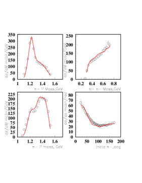
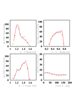
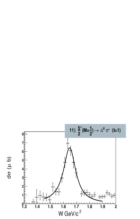
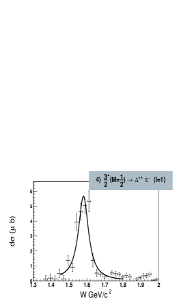
Although the high quality data of two-pion production are now available, the analysis in terms of extraction of resonance parameters has not been fully developed. The theoretical understanding of these complex processes, mainly based on the tree-diagram isobar approach^?, is also very limited and preliminary. Recently, two distinctly different approaches have been applied to analyze the photoproduction and electroproduction data from JLab^?,? and CB-ELSA^?. The first approach is to adjust the parameters of an isobar model^? to fit the fully extracted cross section and polarization asymmetry data ^?,?. The second one is to fit directly the unbinned data event-by-event^?. We describe them in the remaining part of this subsection.

The first approach makes use of knowledge from hadronic production. The energy-dependence of non-resonant processes is parameterized, and resonance photocouplings and hadronic couplings are fixed, if known, e.g. from single pion processes. Resonances in specific partial waves can be introduced to search for undiscovered states. Model parameters are usually fitted to the one-dimensional projections of the multi-dimensional differential cross section. Such a model can lead to a qualitatively good description of the projected data as shown in Fig. 31. The method has been used in the analysis of CLAS electroproduction data ^?. In this analysis a significant disprepancy was found near W = 1.7 GeV between the data and the resonance parametrizations implemented in the fit model. This discrepancy was attributed to either inaccurate hadronic couplings for the well known $P_{13}(1720)$ resonance determined in the analysis of hadronic experiments, or to an additional resonance with $J^{P}={3\over 2}^{+}$ with either $I={1\over 2}$ or $I={3\over 2}$. The discrepancy is best visible in the total cross sections for electroproduction, shown in Fig. 32. The dotted line shows the model predictions using resonance parameters from single pion electroproduction and from the analysis of $\pi N\rightarrow N\pi\pi$ data ^?,?,?. The solid line represents the fit when the hadronic coupling of the $P_{13}(1720)$ to $\Delta\pi$ and $N\rho$ are allowed to vary much beyond the ranges established in the analysis of hadronic data. Alternatively, a new state was introduced with hadronic couplings extracted from the data. Table 5.4.1 summarizes results of the analysis using a single $P_{13}$ with modified hadronic couplings, and a new $P_{I3}$ state with undetermined isospin while keeping the PDG $P_{13}(1720)$ hadronic couplings unchanged. In either case, the fit requires a resonance with hadronic couplings that are significantly different from the ones of the $P_{13}(1720)$ state listed by PDG.

Table 9. PDG parameters for the $P_{13}(1720)$ and parameters resulting from fits to $p\pi^{+}\pi^{-}$ electroproduction data.

Table 9. PDG parameters for the $P_{13}(1720)$ and parameters resulting from fits to $p\pi^{+}\pi^{-}$ electroproduction data.

Mass (MeV) $\Gamma$(MeV) $\Gamma_{\pi\Delta}/\Gamma$(%) $\Gamma_{N\rho}/\Gamma$(%) PDG $P_{13}$ 1725 $\pm$ 20 114 $\pm$ 19 63 $\pm$ 12 19 $\pm$ 9 PDG 1650 - 1750 100 - 200 - 70 - 85 New $P_{I3}$ 1720 $\pm$ 20 88 $\pm$ 17 41 $\pm$ 13 17 $\pm$ 10

The total photoproduction cross section in the left panel of Fig 32 shows a W dependence that is very different from the electroproduction data in the right panel. In particular, the photoproduction has a much higher nonresonant contribution largely due to increased non-resonant $\rho^{\circ}$ production at the photon point. Both data are, however, consistent with a strong resonance near $W=1.72$ GeV in the $P_{13}$ partial wave ^?. The drawback of the approach described above is that when fitting one-dimensional projections of cross sections, correlations between the data sets are lost.

The second approach ^? is based on a partial wave formalism starting from the T matrix at a given photon energy E:

$$T_{fi}(E) = <p\pi^{+}\pi^{-};\tau_{f}|T|\gamma p;E>$$ (128)

$$= \sum_{\alpha}<p\pi^{+}\pi^{-};\tau_{f}|\alpha><\alpha|T|\gamma p;E>$$

$$= \sum_{\alpha}\psi^{\alpha}(\tau_{f})V^{\alpha}(E)~{},$$

where $\alpha$ denotes all intermediate states, and $\tau_{f}$ characterizes the final state kinematics. The decay amplitude $\psi^{\alpha}(\tau_{f})=<p\pi^{+}\pi^{-};\tau_{f}|\alpha>$ is calculated using an isobar model for specific decay channel, e.g. $\Delta^{++}\pi^{-}$, $\Delta^{-}\pi^{+}$, or $p\rho^{\circ}$. The production amplitude $V^{\alpha}=<\alpha|T|\gamma p;E>$ is then fitted at fixed energy using an unbinned maximum likelihood procedure. This method makes use of all information contained in the data, and takes into account all correlations between the variables.

In this analysis a total of 35 partial waves were included in addition to t-channel processes with adjustable parameters. Figure 33 shows intensity distributions in different isobar channels, for the ${5\over 2}(m={1\over 2})$, and ${3\over 2}(m={1\over 2})$ partial waves. Clear signals of the $F_{15}(1680)$ and the $P_{33}(1600)$ are seen, the latter being a not fully established 3-star resonance. In the final analysis the energy-dependence is fitted to a Breit-Wigner form to determine masses and widths of resonant states. This method is closer to a model-independent approach, and can directly ’discover’ new resonances in specific partial waves.

5.4.2 Description of $\gamma p\rightarrow p\pi^{\circ}\pi^{\circ}$ in resonance analyses.

The CB-ELSA collaboration has analysed the $p\pi^{\circ}\pi^{\circ}$ final state using a more model-dependent version of the partial-wave-analysis described above. Here s-channel Breit-Wigner distributions are fitted to the data on an event-by-event basis, therefore retaining the correlations in the data. However, the fit is constrained by the parametrized energy-dependence of the Breit-Wigner function. In Fig. 34 the total cross section for $\gamma p\rightarrow\pi^{\circ}\pi^{\circ}$ is shown as extracted from the integral over all partial waves contributions in comparison to previous data from TABS ^? and GRAAL ^?.

Figure 34: Total cross section of $\gamma p\rightarrow p\pi^{\circ}\pi^{\circ}$ reaction. The connected line is from the preliminary results of a partial wave analysis. The data are from the measurements with TAPS and GRAAL.

Figure 35: Left: Angular distributions of $K^{+}\Lambda$ photoproduction at fixed photon energy $E_{\gamma}$. Right: $K^{+}\Sigma^{\circ}$ angular distributions. Both data sets are from SAPHIR. The lines represent Legendre fits to the data.

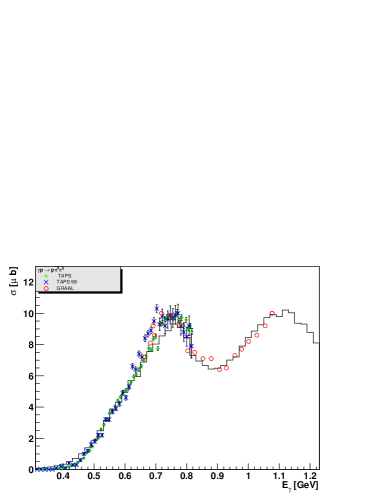
5.5 Kaon production.

Production of kaons from nucleons has long been recognized as a potentially very sensitive tool in the search for excited baryon states ^?. Analyses of the $K\Lambda$ and $K\Sigma$ channels include the isospin selectivity; the $K\Lambda$ final state selects isospin $1\over 2$, similar to the $N\eta$ channel, while $K\Sigma$ couples to both $N^{*}$ and $\Delta^{*}$ resonances. An important tool in resonance studies is the measurement of polarization observables. The self-analyzing power of the weak decay $\Lambda\rightarrow p\pi^{-}$ can be utilized to measure the $\Lambda$ recoil polarization. To make full use of this unique feature large acceptance detectors are needed.

For a long time, the lack of consistent data sets for $K\Lambda$ and $K\Sigma$ production in a wide kinematics range has hampered the use of kaon production in the study of non-strange baryon resonances. Moreover, the interpretation of these data, mainly for charged $K^{+}\Lambda$ and $K^{+}\Sigma^{\circ}$ channels, in terms of $N^{*}$ excitation is complicated by the fact that they may be dominated by the nonresonant particle-exchange processes. Another drawback in comparison to $N\pi$ and $N\pi\pi$ is the relatively small cross section, and the lack of known strong resonances with a dominant coupling to kaon-hyperon channels. This fact makes it more difficult to use strangeness production as a tool in the study of excited baryons, and specifically in the search for new resonances.

Most of the available theoretical models^{?,?,?,?,?,?,?,?,?} for kaon production are based on the tree-diagrams approach, as described in section 4.2. The validity of these tree-diagram models is questionable, as discussed, for example, in a coupled-channel study^? of Kaon photoproduction. We therefore will mainly focus on the status of the data, not on the results from these theoretical models.

5.5.1 Photoproduction of $K^{+}\Lambda$ and $K^{+}\Sigma$

High statistics data of kaon photoproduction covering the resonance region are now available from the SAPHIR ^? and the CLAS ^? collaborations. These new data consist of high statistics angular distributions as well as $\Lambda$ polarization asymmetries, as summarized in table 5.5.1.

Table 10. Summary of hyperon photo- and electroproduction data

Table 10. Summary of hyperon photo- and electroproduction data

Reaction Observable W range $\cos\Theta_{K}^{*}$ range $Q^{2}$ Experiment (GeV) ($GeV^{2}$) $\gamma p\rightarrow\Lambda K$ $d\sigma/d\Omega$ $<2.15$ -0.95 - +0.95 SAPHIR ^? $d\sigma/d\Omega$ $<2.6$ -0.95 - +0.95 SAPHIR ^? $d\sigma/d\Omega$ $<2.3$ -0.85 - +0.85 CLAS ^? $\gamma p\rightarrow\Sigma K$ $d\sigma/d\Omega$ $<2.15$ -0.95 - +0.95 SAPHIR ^? $d\sigma/d\Omega$ $<2.6$ -0.95 - +0.95 SAPHIR ^? $d\sigma/d\Omega$ $<2.3$ -0.85 - +0.85 CLAS ^? $\gamma p\rightarrow K^{+}\vec{\Lambda},\vec{\Sigma}$ P $<2.3$ -0.85 - +0.85 CLAS ^? P $<2.6$ -0.95 - +0.95 SAPHIR ^? $ep\rightarrow eK^{+}\Lambda,~{}\Sigma$ $\sigma_{LT}$,$\sigma_{TT}$, $\sigma_{T}+\epsilon\sigma_{L}$ $<2.5$ -1.0 - +1.0 $<3$ CLAS^? $\vec{e}p\rightarrow eK^{+}\Lambda$ $P_{x}^{\prime}$, $P_{z}^{\prime}$ $<2.15$ -1.0 - +1.0 0.3 - 1.5 CLAS^?

There are significant discrepancies between the CLAS data and the published SAPHIR ^? data, while the new data from SAPHIR ^? are in much better agreement with the CLAS data. We therefore disregard the earlier published data from SAPHIR. Unfortunately, most of the model calculations have been fitted to the published results, and therefore can not be reliably compared to the new data.

The angular distributions for $K^{+}\Lambda$ and $K^{+}\Sigma$ production are shown in Fig. 35. We see that the $K^{+}\Lambda$ data (left panel) show a strong forward peaking for photon energies greater than 1 GeV, indicating the large t-channel contributions. For the $K^{+}\Sigma^{\circ}$ channel (right panel) the angular distribution are more symmetric or “resonance-like” at low energies , but become soemwhat more forward-peaked at energies above 1.3 GeV.

The high statistics of these data allows, for the first time, to identify the structures in the differential cross section that hint the interference between the resonances and the nonresonant backgound. The presence of s-channel resonances is particularly evident in the W-dependence of the differential cross section shown in Figure 36. At the most forward angles (upper panel), two resonance-like structures are visible at $W\approx 1.7$GeV, and at $W\approx 1.95~{}GeV$. The structure at 1.7 GeV could be accomodated by the known states $S_{11}(1650)$, $P_{11}(1710)$, and $P_{13}(1720)$, if the $K\Lambda$ coupling of these states is allowed to vary. From hadronic processes these couplings are very poorly known ^?. At intermediate angles (middle panel) the data indicate a smoother falloff with W, while at backwards angles (lower panel) another resonance-like structure near $W\approx 1.875$ GeV emerges, overlapping with the structure at the higher mass. These distributions reveal complex processes, indicating contributions from more than a single resonance near $W=1.9$ GeV.

Figure 36: W-dependence of $K^{+}\Lambda$ production for several bins in $\cos\theta^{*}_{K}$. Points with full circles are from CLAS. The triangles are older data from SAPHIR. The theoretical curves are from Ref.201 (Guidal/Laget/vdH), Ref.194 (KAON-MAID), and Ref.195 (Janssen).

Figure 37: $\Lambda$ polarization in $K^{+}\Lambda$ photoproduction measured with CLAS. The theoretical curves are the same as those displayed in Fig.36.

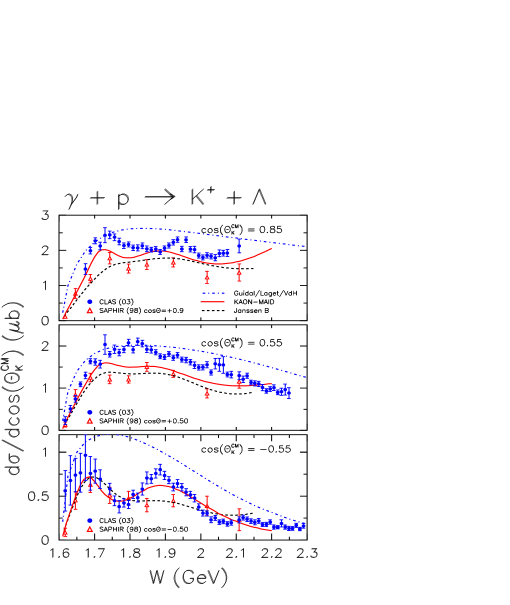
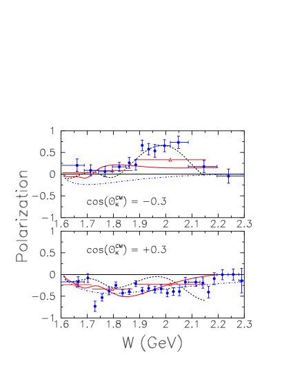
Samples of the $\Lambda$ polarization measured with CLAS are shown in Figure 37. The data show a strong W dependence especially at backward angles (upper panel). Comparing the displayed data at two angles, we can conclude that the angle distributions of the $\Lambda$ polarization change sign from largely negative at forward angles to positive at backward angles.

The three theoretical results displayed in Figs.36 and 37 only describe very qualitatively the main features of the data in the region of the nucleon resonance region.

Figure 38: Cross section from CLAS for $K^{+}\Lambda$ electroproduction at $Q^{2}=0.7$GeV² integrated over to the forward hemisphere (left panel) and backward hemisphere (right panel) in the center-of-mass angle $\theta^{*}_{K}$.

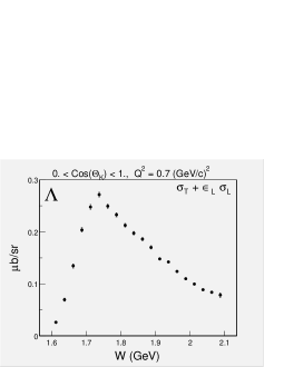
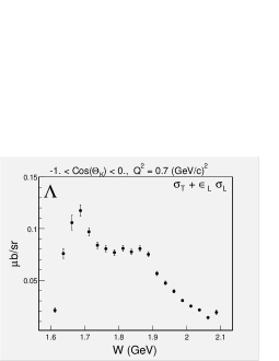
5.5.2 Electroproduction of $K^{+}\Lambda$ and $K^{+}\Sigma$.

Kaon electroproduction is another tool in the study of non-strange nucleon resonances. While the $K^{+}\Lambda$ and $K^{+}\Sigma^{\circ}$ photoproduction cross section exhibits a complex structure of resonant and nonresonant contributions that is difficult to disentangle, some of the resonance contributions in electroproduction may be enhanced at higher $Q^{2}$ due to their slower form factor falloff compared to other resonances, and compared to the background amplitudes. A significant amount of data has become available recently from CLAS ^?,?. In these experiments the electron beam is polarized, and hence the virtual photon also has a net circular polarization.

Figure 38 shows samples of the $K^{+}\Lambda$ production cross sections integrated over either the forward hemisphere (left panel) and backward hemisphere (right panel) at fixed $Q^{2}$. The results reveal resonant behavior near W=1.7 GeV and 1.87 GeV at large angles while at the forward angles the resonant structures are masked by the large non-resonant contributions. The enhancements in the cross section appear in the same invariant mass $W$ range as in photoproduction, and are likely due to the same resonances contributions.

Figure 39: Left: Transferred $\Lambda$ polarization in electroproduction from CLAS. The data have been integrated over all $\phi$ angles. The curves are discussed in the text. Right: Coordinate system defining the $\Lambda$ polarization projections. The curves are predictions of models in Ref. 81 (dotted), Ref. 194 (solid), and Ref. 195 (dot-dashed).

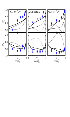
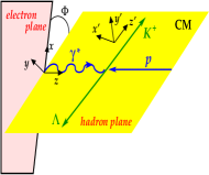
The data of $\Lambda$ recoil polarization have been obtained in measurements with polarized electron beams. The measured total $\Lambda$ recoil polarization can be written as

$$\vec{P}_{\Lambda}=\vec{P}^{\circ}\pm P_{e}\vec{P}^{\prime}$$ (129)

where $P_{e}$ is the electron beam polarization, $\vec{P}^{\circ}$ is the induced polarization which is present without beam polarization, and $\vec{P}^{\prime}$ is the transferred polarization. Figure 39 displays the data of the transferred $\Lambda$ polarization integrated over all $Q^{2}$ for three bins in W. The considered $P_{x^{\prime}}^{\prime}$ and $P_{z^{\prime}}^{\prime}$ are the projections of the polarization vector $\vec{P}^{\prime}$ onto the $x^{\prime}$ and $z^{\prime}$ axes which are also defined in Fig. 39. The data show that the $z^{\prime}$-polarization is large and is rising with $\cos\theta^{*}_{K}$, indicating a t-channel mechanism. On the other hand, the $x^{\prime}$ polarization is large and remains negative throughout the angular range. None of the displayed theoretical results from tree-diagram models ^?,?,? and a Regge model ^? can give an adequate description of the data.

To summarize, production of $K^{+}\Lambda$ and $K^{+}\Sigma^{\circ}$ from protons exhibit evidence of s-channel nucleon resonance contributions in the mass range where no $N^{*}$ or $\Delta^{*}$ resonances have been well established. However, resonances are masked by large t-channel processes. In order to extract reliable information on contributing resonances a better understanding of nonresonant processes is needed. Currently, the most important task is to continue experimentally to establish a broad and solid base of consistent data in the strangeness sector, including extensive differential cross sections, beam and target polarization asymmetries, and polarization transfer measurements. A “complete” measurement of all observables which is needed to unambiguously extract all helicity amplitudes can be achieved ^?,?. This requires use of a polarized photon beam and of a polarized target and the measurement of the hyperon recoil polarization. Experimental effort in this direction will continue with a series of new measurements planned at JLab ^?. On the theoretical side, a dynamical coupled-channel approach, such as that described in section 4.6, must be developed to interpret the extracted $N^{*}$ parameters.

5.5.3 Photoproduction and electroproduction of vector mesons.

The early investigations of photoproduction and electroproduction of vector mesons were mainly in the high energy region where the data can be explained largely by the diffractive Pomeron-exchange mechanism. For the study of nucleon resonances in the $p\omega$ channel, measurements have been performed at ELSA, JLab, and GRAAL to obtain high quality data at energies from production thresholds to $W\sim 2.5$ GeV. In this low energy region, the meson-exchange mechanism plays an important role and must be treated correctly for extracting $N^{*}$ resonance parameters from the data. This is illustrated in Fig. 40. We see that the diffractive Pomeron-exchange(dash-dotted curve) becomes negligible at energies near $\omega$ photoproduction threshold. The s- and u-channel nucleon terms, and $\pi$ and $\eta$ exchanges can account for the main part of the total cross section. The results shown in Fig. 40 are from the tree diagram model described in section 4.2 and no $N^{*}$ excitations are included.

Figure 40: $\gamma p\rightarrow\omega p$ total cross sections. The theoretical curves are from the model of Oh, Titov, and Lee⁸⁶.

Figure 41: Differential cross section for $\gamma p\rightarrow p\omega$ in comparison with model predictions of Oh, Titov, and Lee⁸⁶. The dotted curves include diffractive production and the $\omega\rightarrow\pi^{\circ}\gamma$ vertex. The dashed curves are s-channel resonance contributions using the quark model predictions of Capstick and Roberts.

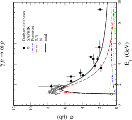
We will here only describe the status of $\omega$ photoproduction in the resonance region( $W<$ 2.5 GeV). The $\rho$ production will not be discussed since $\rho$’s width is very broad and the coupling of the $\rho N$ channel to $N^{*}$ states can be meaningfully defined only in the analysis involving two pion production channels discussed in section 5.4. The $\phi$ photoproduction will also not be covered here since $\phi$ meson has little, if any, contributions from s-channel resonances, as the $s\bar{s}$ quark structure of the $\phi$ makes $N^{*}\rightarrow N\phi$ an OZI forbidden decay.

Quark models that also couple to hadronic channels predict that $\omega$ photoproduction off protons is a promising tool in the search for undiscovered $N^{*}$ states ^?,?. As in the case of $N\eta$ and $K^{+}\Lambda$, the $p\omega$ final state, due to the isoscalar nature of the $\omega$, is only sensitive to isospin $1\over 2$ $N^{*}$ resonances. Experimentally, $p\omega$ production has been measured in both magnetic detectors and in neutral particle detectors. In magnetic detectors the $p\omega$ channel is usually identified through the $\omega\rightarrow\pi^{+}\pi^{-}\pi^{\circ}$ decay. This channel has a 89% branching ratio. Detectors with large acceptance for the detection of photons allows to use the $\omega\rightarrow\pi^{\circ}\gamma$ channel with an 8.5% branching ratio.

The low energy $\omega$ photoproduction data have been obtained ELSA, JLab, and GRAAL. In Fig. 41 we show preliminary differential cross sections from CLAS in comparison with predictions using the model of Oh, Titov, and Lee  ^?. The model contains contributions from diffractive production, $\pi^{\circ}$ exchange, and s-channel $N^{*}$ contributions with the photocouplings from the constituent quark model of Capstick ^?, and the $N^{*}\rightarrow p\omega$ couplings predicted in the model by Capstick and Roberts ^?. At high W and forward angles the cross section is completely dominated by the t-channel processes, i.e. diffractive and pion-exchange contributions. Resonance contributions are evident at larger angles, and they seem to play an important role in the entire mass range covered by the data. The quark model perhaps underestimates the resonance contributions.

The theoretical models for investigating low energy $\omega$ production are still in a developing stage. Most of the calculations, such as those displayed in Fig. 40 and 41, are based on tree-diagrams models, It has been recognized that coupled-channel effects must be accounted for before the model can be used reliably to extract resonance parameters from the data. The importance of the coupled-channel effects on $\omega$ photoproduction has been demonstrated in a one-loop calculation^? based on the dynamical coupled-channel formulation Eqs.(52)-(59). As illustrated in Fig. 42, the photon asymmetry at $E_{\gamma}=1.125$ GeV can be changed drastically if the coupling with the $\pi N$ channel is included in the calculation. The K-matrix coupled-channel model of the Giessen group^?, based on Eq.(71), has also been used to investigate the data from GRAAL. More efforts are needed to improve these theoretical approaches.

Figure 42: Photon Asymmetry of $\omega$ photoproduction at 1.125 GeV. The data are from GRAAL. The dotted curve is from a tree-diagram calculation. The solid curve includes the one-loop coupled-channel effect calculated in Ref.87.

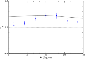
5.6 Comments on the search for “missing” baryon resonanes

The search for all baryon states predicted by the $SU(6)\otimes O(3)$ constituent quark model is without question of the highest importance for the field. This model has the largest number of excitation degrees of freedom of any quark model based on constituent quarks and must form the basis for this search. Hints of possible new states, even claims of discovery have been presented in the analyses of single channel processes ^?,?,?,?,?,? as well as in a coupled-channel analysis ^?.

The analysis of the Giessen group is currently the most extensive in searching for new states. They employ a coupled-channel K matrix model, as described in section 4.4.2, and include all available pion and real photon induced reaction channels, $\gamma N$, $\pi N$, $N\pi\pi$, $N\eta$, $K\Lambda$, $K\Sigma$, $N\omega$. This analysis finds evidence for several new states. While there are clear indications of new resonances near 1900 MeV in some data sets, various analyses do not allow to draw definite conclusions on the partial waves that are needed to explain the data. The Giessen model may be the most promising approach in the search for new states, however, the large amount of data fitted simultaneously with many fit parameters involved makes it difficult to assess the systematic uncertainties in the fit. The dynamical model approaches should be complemented by more experiment-oriented techniques as the one described in section 5.4. Here the binning of data and the evaluation of one-dimensional projections of the multi-dimensional parameter space is replaced by an event-by-event analysis in specific partial waves that retains the correlations in the data for all variables. Theoretical efforts are needed to provide realistic background amplitudes that could strengthen the reliability of these techniques.

6 Concluding remarks and outlook

In the past few years, we have witnessed very significant progress in the study of $N^{*}$ physics. We now have fairly extensive data for $\pi$, $\eta$, $K$, $\omega$ and $\pi\pi$ production channels. Much more data will soon be available. The theoretical models for interpreting these new data and/or extracting the $N^{*}$ parameters have also been developed accordingly.

¿From the analyses of the single pion data in the $\Delta$ region, quantitative information about the $\gamma N\rightarrow\Delta$ transition form factors have been obtained. With the development of dynamical reaction models, the role of pion cloud effects in determining the $\Delta$ excitation has been identified as the source of the long-standing discrepancy between the data and the constituent quark model predictions. Moreover, the $Q^{2}$-dependence of the $\gamma N\rightarrow\Delta$ from factors has also been determined up to about $Q^{2}\sim 6$ (GeV/c)² and found to be in good agreement with the predictions from a dynamical model. The extracted $M1$, $E2$ and $C2$ $\gamma N\rightarrow\Delta$ transition form factors should be considered along with the proton and neutron form factors as benchmark data for testing various hadron models as well as Lattice QCD calculations.

The combined analyses of the $\pi$ and $\eta$ production data had led to a rather quantitative, perhaps nearly model independent, determination of several $N^{*}$ parameters in the second resonance region. However, a correct interpretation of the extracted $N^{*}$ parameters in terms of the current hadron model predictions requires a rigorous investigation of the dynamical coupled-channel effects which are not included in the employed amplitude analyses based on either the K-matrix isobar model or the dispersion relations approach.

The analyses of the $K$, $\pi\pi$ and $\omega$ channels are still in the developing stage. So far, most of the analyses are based on the tree-diagram models with the isobar parameterization for the $N^{*}$ excitations. The final state interactions, as required by the unitarity condition, are either neglected completely or calculated perturbatively using effective Lagrangians. The coupled-channel K-matrix effective Lagrangian model, pioneered by the Giessen Group, looks very promising for extracting the $N^{*}$ parameters from a combined analysis of all channels. But much works are needed to reduce the uncertainties in their non-resonant parameters and to account for the $\pi\pi N$ unitarity condition. For a rigorous interpretation of the extracted resonance parameters in terms of predictions from hadron models or Lattice QCD calculations, the analyses based on the dynamical coupled-channel model, as given in section 4, are indispensable. Progress is being made in this direction.

In the search for new baryon states, progress is being made in developing partial wave analysis procedures that make full use of correlations in the multi-dimensional phase space presented in the complex final states. This effort must be supported by the development of the theory to obtain improved descriptions of background contributions to specific partial waves.

To end, we mention that the progress we have made in the past decade resulted from rather close collaborations between experimentalists and theorists. With much more complex data to be analyzed and interpreted, such collaborations must be continued and extended in order to bring the study of $N^{*}$ physics to a complete success.

Acknowledgments This work was supported in part by the U.S. Department of Energy, Office of Nuclear Physics, under Contract No. W-31-109-ENG-38, and in part under Contract No. DE-AC05-84ER40150.

References

- [1] See, for example, Dynamics of the Standard Model by J.F. Donoghue, E. Golowich, and B. R. Holstein, Cambridge University Press,(1992)
- [2] See, for example, Lattice Gauge Theories: An Introduction by H.J. Rothe, World Scientific Lecture Notes in Physics- Vol.59, World Scientific, Singapore (1997)
- [3] J. Gasser and H. Leutwyler, Phys. Reports, 87, 77 (1982)
- [4] N. Isgur and G. Karl, Phys. Lett. B72, 109 (1977); Phys. Rev. D19, 2653 (1979), Phys. Rev. D23, 817 (181); and earlier rferences therein.
- [5] S. Capstick and N. Isgur, Phys. Rev. D34, 2809 (1986)
- [6] D. B. Leinweber, A. W. Thomas, K. Tsushima, S. V. Wright, Phys.Rev. D61, 074502 (2000).
- [7] S. Aoki et al.Phys. Rev. D 60, 114508 (1999); Yoshinobu Kuramashi for the CP-PACS collaboration, hep-lat/9904003
- [8] D. B. Leinweber, D. H. Lu, and A. W. Thomas, Phys. Rev. D 60, 034014 (1999)
- [9] Y. Chen, S.J. Dong, T. Draper, I. Horváth, F.X. Lee, K.F. Liu, N. Mathur, and J.B. Zhang, hep-lat/0306199 (2004).
- [10] C. Alexandrou et al., arXiv:hep-lat/0307018 (2003)
- [11] L. Ya. Glozman and D.O. Riska, Phys. Rept., 268, 263 (1996).
- [12] L. Ya. Glozman, Z. Rapp, and W. Plessas, Phys. Lett B381, 311 (1996); B. F. Wagenbrunn et al., Phys. Lett. B511, 33 (2001).
- [13] A. Amghar, B. Desplanques, and L. Theussl, Nucl. Phys. A714, 213 (2003).
- [14] F. Coester and D. O. Riska, Nucl.Phys., A728,439 (2003); B. Julia-Diaz, D.O. Riska, and F. Coester, Phys. Rev. C69, 035212 (2004)
- [15] S. Boffi et al., Eur. Phys. J, A14, 17 (2002)
- [16] A. Chodos, R.L. Jaffe, K. Johnson, C.B. Thorn, and V. F. Weisskopf, Phys. Rev. D9, 3471 (1974); D10, 2599 (1974)
- [17] G. E. Brown and M. Rho, Phys. Lett B82, 177 (1979); G.E. Brown, M. Rho, and V. Vento, Phys. Lett. B94, 383 (1979).
- [18] S. Theberge, A.W. Thomas, and G.A. Miller, Phys. Rev. D22, 2838 (1980); D24, 216 (1981).
- [19] R. Bijker, F. Iachello, and A. Leviatan, Ann. Phys. (N.Y.), 236, 69 (1994).
- [20] R. Friedberg and T.D. Lee, Phys. Rev. D15, 1694 (1977); D16, 1096(1977).
- [21] H. B. Neilsen and A. Patkos, Nucl. Phys. B195, 137 (1982); H.J. Pirner, Prog. Part. Nucl. Phys. 29, 33 (1992).
- [22] G. Eckart and B. Schwesinger, Nucl. Phys. A458, 620 (1980)
- [23] See Review by Pieter Maris and Craig D. Roberts, Int.J.Mod.Phys. E12, 297 (2003).
- [24] S. Eidelman et al., Phys. Lett. B592, 1 (2004)
- [25] M. Aguilar-Benitez et al. (Review of Particle Physics 1986), Phys. Lett. B 170 1-350 (1986).
- [26] H. Feshbach, Theoretical Nuclear Physics: Nuclear Reactions (Wiley, New York, 1992).
- [27] H. A. Grunder, et al., Nucl. Phys. A478, 831-846 (1988); H. A. Grunder, Nucl. Phys. A 623 10-15 (1997)
- [28] J. Alcorn, et al., Nucl.Instr.Meth. A 522, 294 -346 (2004)
- [29] B. Mecking et al., Nucl.Instr.Meth. A 503, 513 - 553 (2003).
- [30] J. Friedrich, H. Herminghaus, T. Walcher, Phys. Bl.47, 291 (1991); T. Walcher, Prog. Part. Nucl. Phys. 50, 503-522 (2003)
- [31] K. I. Blomqvist et al., Nucl. Instr. Meth. A 403, 263-301 (1998)
- [32] D. Lohmann et al., Nucl. Instr. Meth.A 343 494-507 (1994) J. Ahrens (A2 Collaboration), Int. Workshop on Physics with GeV electrons and gamma rays, Sendai, Japan, 13-15 Feb. (2001)
- [33] S.M. Dolfini et al., Nucl. Instr. Meth. A 344 571-582 (1994).
- [34] F. Ghio et al., Nucl.Instrum.Meth.A404:71-86 (1998)
- [35] A. D’Angelo et al. (for the GRAAL collaboration), International Conference on the Structure of Baryons, BARYONS2002, Newport News, Virginia, 3-8 Mar 2002, World Scientific, eds. C. Carlson and B. Mecking.
- [36] C.E. Thorn et al., Nucl. Instr. Meth. A 285, 447-458, (1989);
- [37] A. M. Sandorfi et al. (LEGS Spin Collaboration), AIP Conf.Proc.675:651-655, (2003)
- [38] T. Nakano (LEPS Collaboration), Mod. Phys. Lett. A 18, 208 - 214 (2003)
- [39] E. Paul et al., Prog.Part.Nucl.Phys.34, 201-210 (1995)
- [40] U. Thoma, in “Excited Nucleons and Hadronic Structure”, Proceedings of the NSTAR 2000 conference. World Scientific, eds. V. Burkert, L. Elouadrhiri, J. Kelly, R. Minehart.
- [41] Bjorken and Drell, Relativistic Quantum Mechanics, (McGraw-Hill, Inc., 1964)
- [42] A.S. Raskin and T.W. Donnelly, Ann. Phys. (N.Y.) 191, 78 (1989).
- [43] W.-T. Chiang, S.N. Yang, L. Tiator, and D. Drechsel, Nucl. Phys. A 700, 429 (2002)
- [44] G. Knöchlein, D. Drechsel, and L. Tiator, Z. Phys. A 352, 327 (1995)
- [45] M. Pichowsky, C. Savkli and F. Tabakin, Phys. Rev. C 53, 593 (1996)
- [46] A. Donnachie, pages 1 - 185, Vol.5, High Energy Physics, edited by E.H.S. Burhop (Academic Press), 1972
- [47] F. Chew, M. Goldberger, F. Low, and Y. Nambu, Phys. Rev. 106, 1345 (1957).
- [48] R.L. Walker, Phys. Rev. 182, 1729 (1969)
- [49] F. A. Berends, A. Donnachie, and D. L. Weaver, Nucl. Phys. B4,1; B4, 54; B4, 103.
- [50] O. Hanstein, D. Drechsel, and L. Tiator, Nucl. Phys. A632, 561 (1998)
- [51] I. G. Aznauryan, Phys. Rev. C57, 2727 (1998)
- [52] I. G. Aznauryan, Phys. Rev. C67, 015209 (2003)
- [53] I. G. Aznauryan, Phys. Rev. C68, 065204 (2003)
- [54] M.G. Olsson and E.T. Osypowski, Nucl. Phys.B87, 399 (1975); Phys. Rev. D17, 174 (1978).
- [55] R. M. Davidson and N.C. Mukhopadhyay, Phys. Rev. D42, 20 (1990); R. M. Davidson, N.C. Mukhopadhyay, and R.S. Wittman, Phys. Rev. D43, 71 (1991).
- [56] R.A. Arndt, I.I. Strakovsky, R.L. Workman, and M.M. Pavan, Phys. Rev. C52, 2120 (1995); R.A. Arndt, I.I. Strakovsky, R.L. Workman, Phys. Rev. 53, 430 (1996); R.A. Arndt, I.I. Strakovsky, R.L. Workman, Int. J. Mod. Phys. A18, 449-455 (2003)
- [57] D. Drechsel, O. Hanstein, S.S. Kamalov, and L. Tiator, Nucl. Phys. A645, 145 (1999)
- [58] D. M. Manley, Int. J. of Mod. Phys., A18, 441 (2003);
- [59] D.M. Manley and E.M. Saleski, Phys. Rev. D45, 4002 (1992).
- [60] Feuster and U. Mosel, Phys. Rev. C58, 457 (1998); Phys. Rev. C59, 460-491 (1999); G. Penner and U. Mosel, Phys. Rev. C66, 055211 (2002); C66, 055212 (2002).
- [61] R.E. Cutkosky, C.P. Forsyth, R.E. Hendrick, and R.L. Kelly, Phys. Rev. D20, 2839 (1979).
- [62] M. Batinic, I. Slaus, and A. Svarc, Phys. Rev. C51, 2310 (1995)
- [63] T.P. Vrana, S.A. Dytman, and T.-S. H. Lee, Phys. Rept. 328, 181 (2000).
- [64] Tanabe and Ohta, Phys. Rev. C31, 1876 (1985).
- [65] S. N. Yang, J. Phys. G 11, L200 (1985)
- [66] S. Nozawa, B. Blankenleider, and T.-S. H. Lee, Nucl. Phys. A513, 459 (1990)
- [67] F. Gross and Y.Surya, Phys. Rev. C47, 703 (1993); Y.Surya and F. Gross, Phys. Rev. C 53, 2422 (1996).
- [68] T. Sato and T.-S. H. Lee, Phys. Rev. C 54, 2660 (1996)
- [69] Yoshimoto, T. Sato, M. Arima, and T.-S. H. Lee, Phys. Rev. C61 065203 (2000).
- [70] T. Sato and T.-S. H. Lee, Phys. Rev. C63, 055201 (2001).
- [71] Kamalov and S.N. Yang, Phys. Rev. Lett. 83, 4494 (1999).
- [72] G.-Y. Chen, S.S. Kamalov, S. N. Yang, D. Drechsel, and L. Tiator, Nucl. Phys. A723, 447 (2003).
- [73] S.S. Kamalov, S. N. Yang, D. Drechsel, O. Hanstein, and L. Tiator, Phys, Rev, C64, 032201(R) (2001),
- [74] W.-T. Chiang, F. Tabakin, T.-S. H. Lee and B. Saghai, Phys. Lett. B517, 101 (2001).
- [75] M. G. Fuda and H. Alharbi, Phys. Rev. C68, 064002 (2003).
- [76] T.-S. H. Lee, A. Matsuyama, and T. Sato, in preparation
- [77] N. Kaiser, P.B. Siegel, and W. Weise, Nucl. Phys. A594, 325 (1995); N. Kaiser, T. Waas, and W. Weise, Nucl. Phys. A612, 297 (1997).
- [78] E. Oset and A. Ramos, Nucl. Phys. A635, 99 (1998).
- [79] R.A. Adelseck, C. Bennhold, and L.E. Wright, Phys. Rev. C32, 1681 (1985)
- [80] R.A. Adeleck and B. Saghai, Phys. Rev. C42, 108 (1990).
- [81] R.A. Williams, C.R. Ji, and S. R. Cotanch, Phys. Rev. C46, 1617 (1992).
- [82] J.C. David, C. Fayard, G.H. Lamot, and B. Saghai, Phys. Rev. C53, 2613 (1996)
- [83] Z. Li and B. Saghai, Nucl. Phys. A644, 345 (1998)
- [84] T. Mart and C. Bennhold, Phys. Rev. C61, 12201 (2000).
- [85] Q. Zhao, Z. Li, and C. Bennhold, Phys. Rev. C 58, 2393 (1998); Q. Zhao, ibid. 63, 025203 (2001).
- [86] Y. Oh, A. Titov, and T.-S. H. Lee, Phys. Rev. C63, 025201 (2001).
- [87] Y. Oh and T.-S. H. Lee, Phys. Rev. C66, 045201 (2002).
- [88] M. Guidal, J.M. Laget, and M. Vanderhaeghen, Nucl. Phys. A627, 645 (1997).
- [89] W.-T. Chiang, S.N. Yang, L. Tiator, M. Vanderhaeghen, and D. Drechsel, Phys. Rev. C68, 045202 (2003).
- [90] J. C. Nacher and E. Oset, Nucl. Phys. A674, 205 (2000)
- [91] M. Ripani et al., Nucl. Phys. A672, 220 (2000); V. Mokeev et al., Phys. of Atomic Nucl. 64, 1292 (2001)
- [92] T.-S. H. Lee, unpublished.
- [93] A. Kiswandhi, S. Capstick, and S.A. Dytman, Phys. Rev. C69, 025205 (2004)
- [94] M. Goldberger and Watson, Collision Theory, Robert E. Krieger Publishing Company (1975)
- [95] C.T. Hung, S.N. Yang and T.-S. H. Lee, Phys. Rev. C64, 034309 (2001).
- [96] We use Edmond’s convention .
- [97] T. deForest and J.D. Walecka, Adv. Phys. 15, 1 (1966).
- [98] E. Amaldi, S. Fubini, and G. Furlan, Springer Tracts in Modern Physics, 83 (1979)
- [99] D.H. Lu, S.N. Yang, and A. W. Thomas, Nucl.Phys. A684, 296 (2001).
- [100] M. Araki and I.R. Afnan, Phys. Rev. C36, 250 (1987).
- [101] S. Capstick, Phys. Rev. C46, 2864 (1992);
- [102] S. Capstick and W. Roberts, Phys. Rev. C49, 4570 (1994); Phys. Rev. D 57, 4301-4309 (1998)
- [103] S. Capstick and W. Roberts, Phys. Rev. D58 074011 (1998)
- [104] O. Krehl, C. Hanhart, S. Krewald, and J. Speth, Phys. Rev. C62, 025270 (2000)
- [105] D. Schwela and R. Weizel, Z. Phys. 221, 71 (1969)
- [106] J. B.Bell, Phys. Rev. 124, 2014 (1961)
- [107] R. Omnes, Nuovo Cim. 8, 316 (1958)
- [108] R.L. Crawford, Nucl. Phys. B97, 125 (1975)
- [109] F. Foster and G. Hughes, Rept. Prog. Phys.46, 1445-1489 (1983)
- [110] B. Krusche and S. Schadmand, Prog.Part.Nucl.Phys. 51, 399-485 (2003)
- [111] G. Blanpied et al., Phys. Rev. C 61, 024604 (2000).
- [112] R. Beck et al., Phys. Rev. Lett. 78, 606 (1997); R. Beck et al., Phys. Rev. C 61, 035204 (2000).
- [113] J. Ajaka et al., Phys. Lett. B475, 372-377 (2000); O. Bartalini et al, Phys. Lett. B544, 113-120 (2002)
- [114] J. Ahrens et al., Phys. Rev. Lett. 84, 5950 (2000);
- [115] J. Ahrens et al., Phys. Rev. Let. 88, 232002 (2002).
- [116] A. Arndt et al., p. 467, NSTAR 2001, Proceedings of the Workshop on the Physics of Excited Nucleons, Edited by D. Drechsel and L. Tiator, World Scientific (2001)
- [117] V. Frolov, et al., Phys.Rev. Lett.82, 45 (1999).
- [118] G. Laveissière, et al., nucl-ex/0308009 (2003).
- [119] P. Stoler et al., JLab Experiment E-01-002 (2002); P. Stoler, Phys. Rev. Let. 91, 172303 (2003)
- [120] H. Breuker et al., Z. Phys. C13, 113 (1982); H. Breuker et al., Nucl. Phys. B146, 285-302 (1978).
- [121] J. C. Alder et al., Nucl. Phys. B99 1 (1975).
- [122] E. Evangelides et al., Nucl. Phys. B71 381 (1974);
- [123] H. Breuker et al., Z. Phys. C17, 121 (1983).
- [124] J. V. Morris et al., Phys. Lett. B73 495 (1978); J. V. Morris et al., Phys. Lett. B86 211 (1979).
- [125] H. Egiyan et al. (CLAS Collaboration); Workshop on the Physics of Excited Nucleons, Pittsburgh, Pennsylvania, 9-12 Oct 2002, World Scientific, eds. S. A. Dytman and E. S. Swanson; H. Egiyan, et al. (CLAS collaboration), to be submitted to Phys. Rev. C, (2004).
- [126] K. Joo, et al. (CLAS collaboration), Phys. Rev. Lett. 88, 122001 (2002).
- [127] K. Joo, et al., (CLAS collaboration) Phys. Rev. C 68, 032201 (2003)
- [128] P. Bartsch et al., Phys. Rev. Lett. 88, 142001 (2002)
- [129] C. Kunz et al., (OOPS collaboration), Phys. Lett. B 564, 21-26 (2003)
- [130] K. Joo et al. (CLAS collaboration), International Conference on the Structure of Baryons, BARYONS2002, Newport News, Virginia, 3-8 Mar 2002, World Scientific, eds. C. Carlson and B. Mecking.
- [131] R. Gothe, Workshop on the Physics of Excited Nucleons, Pittsburgh, Pennsylvania, 9-12 Oct 2002, World Scientific, eds. S. A. Dytman and E. S. Swanson.
- [132] V. Burkert, R. Minehart, P. Stoler, M. Taiuti, et al., JLab experiment E01-002.
- [133] P. Bosted, V. Frolov, M. Jones, V. Kubarovski, P. Stoler et al., JLab experiment E99-107.
- [134] S. Frullani, J. Kelly, A. Sarty, et al., JLab experiment E99-011 (1991).
- [135] R. De Vita, et al. (CLAS Collaboration), Phys. Rev. Lett. 88, 082001-1 (2002).
- [136] A. Biselli et al., Phys. Rev. C68, 035202 (2003);
- [137] A. Biselli et al. (CLAS collaboration), to appear in proceedings of NSTAR2004 workshop, March 24-27, 2004, Grenoble, France.
- [138] L. Tiator, et al., nucl-th/0310041
- [139] L.C. Smith (for the CLAS collaboration), Talk presented at the NSTAR2004 workshop, March 24-27, 2004, Grenoble, France.
- [140] I. Aznauryan, V. Burkert, H. Egiyan, K. Joo, R. MInehart, and L.C. Smith; nucl-th/0407021 (2004).
- [141] C.S. Armstrong, et al., Phys. Rev. D60, 052004 (1999).
- [142] M. Dugger, et al., (CLAS collaboration) Phys. Rev. Lett. 89, 222002 (2002)
- [143] V. Crede et al. (CB-ELSA collaboration), arXiv:hep-ex/0311045 (2003)
- [144] F. Klein et al., JLab Experiment E02-112.
- [145] D. Rebreyend, Proceedings of NSTAR 2002, Pittsburg, 2002, eds: S. A. Dytman, E.S. Swanson.
- [146] V. Kuznetsov, private communication.
- [147] J. Ahrens et al. (A2 collaboration), Eur. Phys. J. A17 241-244 (2003)
- [148] B. Krusche et al., Phys. Rev. Lett. 74, 3736-3739 (1995)
- [149] A. Bock et al., Phys. Rev. Lett. 81, 534-537 (1998); J. Price et al., Phys. Rev. C51, 2283-2287 (1995)
- [150] R.A. Arndt, I.I. Strakovsky and R.L. Workman, Phys. Rev. C 53, 430 (1996)
- [151] R. Thompson, et al., (CLAS collaboration), Phys. Rev. Lett 86, 1702 (2001)
- [152] F. Renard et al., Phys. Lett. B 258, 215 (2002)
- [153] J. Ajaka, et al., Phys. Rev. Lett. 81, 1797 (1998).
- [154] H. Denizli et al., International Conference on the Structure of Baryons, BARYONS2002, Newport News, Virginia, 3-8 Mar 2002, World Scientific, eds. C. Carlson and B. Mecking.
- [155] G. Höhler, PiN Newslett.14, 168-184 (1998)
- [156] N. Kaiser, P.B. Siegel, and W. Weise, Phys. Lett. B362, 23-28 (1995)
- [157] S. J. Dong et al., arXiv:hep-ph/0306199 (2003)
- [158] Workshop on the Physics of Excited Nucleons, Pittsburgh, Pennsylvania, 9-12 Oct 2002, World Scientific, eds. S. A. Dytman and E. S. Swanson.
- [159] Wen-Tai Chiang, et al., Phys. Rev. C68, 045202 (2003)
- [160] Wen-Tai Chiang, Shin Nan Yang, L. Tiator, D. Drechsel, Nucl. Phys. A700, 429 (2002)
- [161] B. Saghai and Z.P. Li, Eur. Phys. J. A 11, 217-230 (2001)
- [162] J.-C. Alder et al., Nucl. Phys. B91 386 (1975).
- [163] W. Brasse et al., Nucl. Phys. B139, 37 (1978); Z. Phys. C22, 33-38 (1984).
- [164] U. Beck et al., Phys. Lett. B51, 103-105 (1974)
- [165] H. Breuker et al., Phys. Lett. B74, 409-412 (1978)
- [166] R.A. Arndt, I.I. Strakovsky, and R.L. Workman, Phys. Rev. C 53, 430-440 (1996)
- [167] R.A. Arndt, W.J. Briscoe, I.I. Strakovsky, and R.L. Workman, Phys. Rev. C 66, 055213 (2002)
- [168] R. Workman, A. R. Arndt, I.I. Strakovsky, Phys. Rev. C62, 048201 (2000)
- [169] P. Koniuk and N. Isgur, Phys. Rev. D 21, 1868-1886 (1980)
- [170] P. Koniuk and N. Isgur, Phys. Rev. Lett.44 845 (1980)
- [171] Z.P. Li, V. Burkert, and Zh. Li, Phys. Rev. D 46, 70, (1992)
- [172] y M. Warns, H. Schröder W. Pfeil, H. Rollnik (Bonn U.) Z. Phys. C45, 627 (1990)
- [173] S. Capstick and B.D. Keister, Phys. Rev. D 51, 3598-3612, (1995)
- [174] F. Cardarelli and S. Simula, Phys. Rev. Lett. 62, 06520 (2000)
- [175] M. Giannini, E. Santopinto, and A. Vassallo, Prog. Part. Nucl. Phys. 50, 263-272 (2003)
- [176] F. Cano and P. Gonzalez, Phys. Lett. B431, 270-276 (1998)
- [177] F. E. Close, Z.P. Li Phys. Rev. D42, 2194-2206 (1990)
- [178] V. Burkert, R. De Vita, M. Battaglieri, V. Mokeev, and M. Ripani, Phys. Rev. C 67, 035204 (2003)
- [179] A.J.G. Hey and J. Weyers, Phys. Lett. 48B, 69 (1974).
- [180] W.N. Cottingham and I.H. Dunbar, Z. Phys. C2, 41 (1979).
- [181] F. E. Close, An Introduction to Quarks and Partons, Academic Press/London (1979).
- [182] V. Burkert et al., (CLAS Collaboration), JLab experiment E099-108.
- [183] U. Thoma, Workshop on the Physics of Excited Nucleons, Pittsburgh, Pennsylvania, 9-12 Oct 2002, World Scientific, eds. S. A. Dytman and E. S. Swanson.
- [184] M. Ripani, V. D. Burkert, V. Mokeev, et al. (CLAS Collaboration), Phys. Rev. Lett. 91, 022002 (2003)
- [185] V.I. Mokeev, et al., Proceedings of the NSTAR2004 Conference, Grenoble, March 24-27, 2004, to be published in World Scientific.
- [186] M. Bellis, et al. (CLAS collaboration), to appear in proceedings of NSTAR2004 workshop, March 24-27, 2004, Grenoble, France.
- [187] M.Q. Tran et al., Phys. Lett. B 445, 20 (1998)
- [188] Y. Assafiri et al., Phys. Rev. Lett. 90, 222001 2003)
- [189] M. Wolf et al., Eur. Phys. J 9, 5 (2000)
- [190] F. Harter et al., Phys. Lett. B 401 229 (1997)
- [191] V. Mokeev, et al., Phys.Atom.Nucl. 64, 1292-1298 (2001)
- [192] V. Burkert, et al., Phys. Atom. Nucl. 66, 2149-2158 (2003).
- [193] H. Haberzettl, C. Bennhold and W. Mart, Phys. Rev. C58, 40-44 (1998)
- [194] W. Mart and C. Bennhold, and H. Haberzettl, PiN Newslett.16, 86 (2002)
- [195] S. Janssen, J. Ryckebusch, D. Debruyne, and T.V. Cauteren, Phys. Rev. C65, 015201 (2001)
- [196] K. H. Glander, et al., Eur. Phys. J. A19, 251 - 273 (2004)
- [197] J. W. C. Mc Nabb, et al. [CLAS Collaboration], Phys. Rev. C69 042201 (2004), arXiv:nucl-ex/0305028
- [198] G. Niculescu (CLAS Collaboration), International Conference on the Structure of Baryons, BARYONS2002, Newport News, Virginia, 3-8 Mar 2002, World Scientific, eds. C. Carlson and B. Mecking.
- [199] M. Mestayer et al., (CLAS Collaboration), Proceedings of PANIC’99, Uppsala, 10-16 June, 1999, publ. Elsevier Science, eds. G. Fäldt, B. Höistad, and S. Kullander.
- [200] D. S. Carman et al. (CLAS Collaboration), Phys. Rev. Lett. 90, 131804 (2003).
- [201] M. Guidal, J.M. Laget, and M. Vanderhaeghen, Phys. Rev. C68, 058201 (2003).
- [202] B. Saghai and Z.P. Li, Workshop on the Physics of Excited Nucleons, Pittsburgh, Pennsylvania, 9-12 Oct 2002, World Scientific, eds. S. A. Dytman and E. S. Swanson, arXiv:nucl-th/0305004.
- [203] I.S. Barker, A. Donnachie, and J.K. Storrow, Nucl. Phys. B79, 431
- [204] I.S. Barker, A. Donnachie, and J.K. Storrow, Nucl. Phys. B95, 347
- [205] P. Eugenio, F. Klein, L. Todor, et al., JLab Experiment E02-112.
- [206] M. Kirchbach, Mod. Phys. Lett. A12, 3177-3188 (1997) ; M. Kirchbach, Int. J. Mod. Phys.A15 1435-1451 (2000); M. Kirchbach, M. Moshinsky, and Yu. F. Smirnov, Phys. Rev. D64, 114005 (2001); M. Kirchbach, arXiv:nucl-th/0303049 (2003).
- [207] D.G. Ireland, S. Janssen, and J. Ryckebusch, Phys. Lett. B 562 51-56 (2003)