Abstract

The experiment aiming at the simultaneous determination of the two transversal polarisation components of electrons emitted in the decay of free, polarised neutrons is in progress at the Paul Scherrer Institute (Villigen, Switzerland). The non-zero value of $R$ coefficient, proportional to the polarisation component, which is perpendicular to the plane spanned by the spin of the decaying neutron and the electron momentum, would prove a violation of time reversal symmetry and thus physics beyond the Standard Model. The planned accuracy of the measurement is of order 0.005. To reach this value, the systematic effects in the experiment have to be controlled on a similar level of accuracy. The emphasis of this master’s thesis is put on the search of systematic effects by the means of dedicated Monte Carlo simulation, based on extended Geant4 package. Implementation details are discussed and the new added features are tested. Finally, the $\beta$ decay asymmetry induced systematic effect, resulting in false contribution to $R$-coefficient is recognised and investigated.

Streszczenie

W Instytucie Paula Scherrera (Villigen, Szwajcaria) prowadzony jest eksperyment maj_⸦acy na celu jednoczesny pomiar obu poprzecznych składowych polaryzacji elektronów emitowanych w rozpadzie swobodnych, spolaryzowanych neutronów. Niezerowa wartość wspólczynnika $R$, proporcjonalnego do tej składowej polaryzacji, która jest prostopadła do płaszczyzny tworzonej przez spin neutronu i p_⸦ed elektronu, świadczyłaby o istnieniu procesu łami_⸦acego symetri_⸦e wzgl_⸦edem odwrócenia czasu, wykraczaj_⸦acego poza obecnie uznawan_⸦a  struktur_⸦e  Modelu Standardowego. Aby móc osiagn_⸦ać planowan_⸦a dokładność pomiaru (0.005), konieczne jest oszacowanie możliwych efektów systematycznych. W poniższej pracy magisterskiej nacisk położono na poszukiwanie efektów systematycznych przy pomocy specjalnie do tego celu stworzonej symulacji Monte Carlo, opartej na rozszerzonym pakiecie Geant4. Omówione s_⸦a szczególy implementacji oraz wyniki testów nowych, dodanych do pakietu funkcji. Opisano też i przeanalizowano odkryty efekt systematyczny, spowodowany asymetri_⸦a rozpadu $\beta$ i wnosz_⸦acy fałszywy wkład do mierzonego wspólczynnika $R$.

Kraków 2004

Chapter 1 Introduction

From the nuclear physicist’s point of view next few years are going to be really interesting. On the one hand, the Standard Model (SM) has still an impressive predictive power and so far in particle physics there has been a total agreement with experimental evidence. On the other hand, SM is not believed to be a complete theory. Nowadays there are plenty of much more elegant new theories or at least extensions of the SM. Moreover, there is one huge discrepancy between its predictions and astronomical observations, namely the baryon asymmetry of the Universe which is by a factor $10^{8}$ larger than expected. In other words, according to the SM, large concentrations of baryon matter, such as galaxies, could not have even existed and the Universe should have been more like a uniform “sea” of radiation.

One of very few reasonable explanations of this paradox requires the breaking of combined charge conjugation and parity symmetry ($\cal CP$). Assuming that $\cal CPT$ symmetry (combined time-reversal symmetry $\cal T$ and $\cal CP$) is conserved, what is required by all renormalisable quantum field theories, $\cal CP$ violation implies $\cal T$ violation. Both $\cal CP$ or $\cal T$-violating processes have been so far observed only in the neutral $K$ and $B$ meson systems and their mechanism has been already included in the SM by introducing a quark mixing mechanism. However, to explain the problem of baryon asymmetry additional sources of $\cal CP$ or $\cal T$ breaking have to be found.

Measurements of vector correlations in particle decays and searching for electric dipole moments of particles belong to the most promising ways to discover new $\cal T$-violating processes not predicted by the SM. For both types of experiments, physics of cold neutrons is especially interesting, due to the availability of high intensity polarised beams. The experiment aimed at the determination of the $R$-correlation parameter (mixed product of neutron spin, electron momentum and electron spin) in the $\beta^{-}$ decay of free, polarised cold neutrons will start data taking this summer at the Paul Scherrer Institute (Villigen, Switzerland). It is going to be the first such a measurement for the decay of free neutrons, bearing a potential to detect either a non-standard value, inconsistent with zero or to provide important constraints for the $\cal T$-violating scalar and tensor couplings in the semileptonic weak interactions.

The subject of this thesis is the analysis of experimental uncertainties in the $R$-correlation experiment. The measurement is planned to achieve accuracy of 0.005, with the main contribution to the error coming from the counting statistics. In order to perform detailed study of possible systematic effects, a dedicated Monte Carlo simulation (based on Geant4 package) has been created and exploited.

Before the main goal could have been completed, the following intermediate steps had to be fulfilled:

• Unification of all existing parts of the source code in one general simulation of the whole experiment

• Implementation of new geometry of the experimental setup

• Modification of Geant4 libraries to include electron polarisation transport and the spin dependent neutron $\beta^{-}$ decay

• Further software development and optimisation

• Actual simulations and data analysis

The next chapter briefly describes the theoretical aspects of the neutron $\beta^{-}$ decay, which are essential for understanding the principle of the experiment. In addition, interactions of electrons with matter and foundations of the polarisation theory are sketched, especially the formulae used in the simulation. The third chapter contains detailed information about the measurement itself and the description of the experimental apparatus. In further chapters, the Monte Carlo simulation and its results are presented and discussed. Appendices contain practical information on the software usage.

Chapter 2 Theory

2.1 The neutron $\beta^{-}$ decay and angular correlations

The neutron is about 0.2% more massive than a proton, which translates to an energy difference of 1.29 M eV . Therefore, from the energy conservation law, it is possible for a free neutron to decay with the emission of an electron and an electron anti-neutrino

$$n\rightarrow p+e^{-}+\mathrm{bar}{\nu}_{e}\mbox{\ \ \ \ \ Q = 782.2$\,\pm\,$0.1 \mathrm{ k }\mathrm{ eV }}.$$

Because it is a three-particle decay, produced electrons have continuous distribution of momentum and energy (Fig. 2.1) given by

$$W_{1}(p_{e}) \propto F(Z,p_{e})p_{e}^{2}(p_{max}-p_{e})^{2},$$ (2.1)

$$W_{2}(E_{e}) \propto \frac{2\pi\alpha}{\beta}\frac{1}{1-e^{-\frac{2\pi\alpha}{\beta}}}p_{e}E_{e}(E_{max}-E_{e})^{2},$$ (2.2)

where $F(Z,p_{e})$ is the Fermi function, $\beta=\frac{p_{e}}{E_{e}}$, $E_{max}=1.29\leavevmode\nobreak\ \mathrm{M}\mathrm{eV}$, $p_{max}=1.19\leavevmode\nobreak\ \mathrm{M}\mathrm{eV}/c$ and $\alpha$ is the fine structure constant.

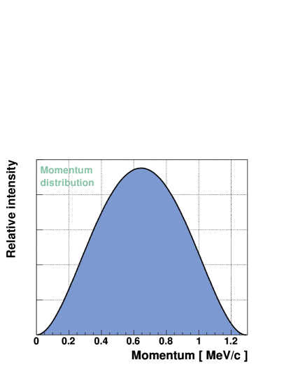
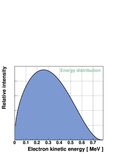
Figure 2.1: The observed momentum and energy distributions for the $\beta$ electron

The decay of neutrons involves the weak interaction (see Fig. 2.2), which, according to the theoretical description embedded in the SM (Feynman and Gell-Mann, 1958), has the strict vector-axial form ($V-A$).

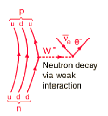
Figure 2.2: The neutron decay as the transformation of one of the neutron’s down quarks into an up quark.

To find $\cal{T}$-violating effects in $\beta$ decay, one has to measure at least three vector or axial-vector quantities, namely momenta and spins of the different particles involved in the decay ($e$, $\nu_{e}$, $p$, $n$); the quantities, which are all reversed under the time reversal operation. Rotational invariance requires the observables to be scalars or pseudo-scalars, therefore the lowest order $\cal{T}$-violating combination of spins and momenta appears in the form of the mixed triple product. From the experimentally accessible quantities, four such products can be formed (see the Tab. 2.1).

Correlation	Broken symmetry	Definition
$R$	$\cal{T}$, $\cal{P}$	$\vec{J}\cdot\left(\vec{p}_{e}\times\vec{\sigma}\right)$
$D$	$\cal{T}$	$\vec{J}\cdot\left(\vec{p}_{e}\times\vec{p}_{\nu_{e}}\right)$
$V$	$\cal{T}$, $\cal{P}$	$\vec{J}\cdot\left(\vec{P}\times\vec{\sigma}\right)$
$L$	$\cal{T}$	$\vec{P}\cdot\left(\vec{p}_{e}\times\vec{\sigma}\right)$

Table 2.1: $\cal{T}$-violating triple products. $\vec{J}$ is the neutron spin, $\vec{p}_{e}$ and $\vec{\sigma}$ are the momentum and spin of the electron, respectively, $\vec{P}$ denotes the proton momentum and $\vec{p}_{\nu_{e}}$ stands for the momentum of the neutrino.

From now on let’s concentrate on the planned experiment, in which the momentum and spin of electrons from decaying oriented neutrons will be measured. The decay probability distribution suitable for this case has been derived by Jackson [6]

$$W\propto\left[1+b\frac{m}{E_{e}}+A\frac{\vec{\left<J\right>}\cdot\vec{p}_{e}}{E_{e}}+G\frac{\vec{\sigma}\cdot\vec{p}_{e}}{E_{e}}+N\vec{\sigma}\cdot\vec{\left<J\right>}+Q\frac{\vec{\sigma}\cdot\vec{p}_{e}}{E_{e}+m}\frac{\vec{\left<J\right>}\cdot\vec{p}_{e}}{E_{e}}+R\frac{\vec{\left<J\right>}\cdot\left(\vec{p}_{e}\times\vec{\sigma}\right)}{E_{e}}\right]$$ (2.3)

where

$b$ is the Fierz interference coefficient, $A$ = $-2\frac{\lambda^{2}+\lambda}{1+3\lambda^{2}}$ is the decay asymmetry parameter, $G$ = $-1$, $Q$ = $2\frac{1+\lambda}{3+\lambda^{2}}$, $N$ = $-A\frac{m_{e}}{E_{e}}$, $\lambda$ denotes the coupling constants ratio $C_{A}/C_{V}$.

Using $\lambda=-1.267$ (see [20]), one retrieves values:

$$A=-0.1162,\mbox{\ \ \ \ }Q=-0.1160.$$

The coefficient $b$ vanishes if there are no scalar and tensor couplings, therefore the zero value has been used. The formula 2.3 is the consequence of the interaction Hamiltonian density for weak currents, as given by Yang and Lee [7]. As can be seen on the Fig. 2.3, $R$ and $N$ parameters are proportional to orthogonal components of the transversal electron polarisation.

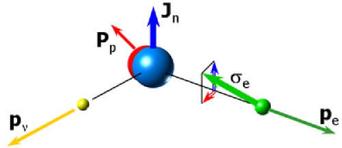
Figure 2.3: Directions of spins of the neutron and the electron from the $\beta^{-}$ decay. In the $R$-correlation experiment the transversal component of the electron polarisation will be measured

However, only the $R$-correlation reveals direct sensitivity to the existence of exotic $\cal T$-violating scalar and tensor couplings in the semileptonic weak interactions.

2.2 Polarisation theory

The following brief review of the polarisation theory formalism is based on the Refs. [9], [16] and [10]. The Stokes parameters are defined below for the general case and for the specific case of electrons. When used as a four-vector, the Stokes parameters allow the ordinary polarisation-sensitive cross sections to be written in matrix form, which is a very convenient representation for the description of polarisation phenomena.

2.2.1 Stokes parameters

In quantum mechanics the wave function describing a pure state of polarisation can be expanded in a complete set of orthonormal eigenfunctions. For particles of spin $\frac{1}{2}$ this expansion contains only two terms,

$$\psi=a_{1}\psi_{1}+a_{2}\psi_{2}.$$ (2.4)

The wave functions describing pure states may be chosen in the form

$$\psi_{1}=\left(\begin{array}[]{c}1\\ 0\end{array}\right) \psi_{2}=\left(\begin{array}[]{c}0\\ 1\end{array}\right).$$ (2.9)

Thus, the general wave function describing the beam is given by

$$\psi=\left(\begin{array}[]{c}a_{1}\\ a_{2}\end{array}\right).$$ (2.10)

In the specific case of the electron, the explicit form of this function can be found by solving the Dirac equation. As a result, one can achieve two independent solutions (spin “$+$” and spin “$-$”) for the electron and two for the positron. Choosing the solutions for the electron, one immediately obtains wave functions (2.9).

In the rest frame of the electron the four-component solutions of the Dirac equation are reduced to two-component spinors, leading to the following expressions for the expectation value of the unit matrix and the expectation values of the Pauli spin operators:

$$I=\langle\psi\mid I\mid\psi\rangle=\left(\begin{array}[]{cc}a_{1}^{*}&a_{2}^{*}\end{array}\right){{\left(\begin{array}[]{cc}{1}&{\,\,0}\\ {0}&{\,\,\,1}\end{array}\right)}}\left(\begin{array}[]{c}a_{1}\\ a_{2}\end{array}\right) = a_{1}a_{1}^{*}-a_{2}a_{2}^{*}\,,$$

$$P_{1}=\langle\psi\mid\sigma_{z}\mid\psi\rangle=\left(\begin{array}[]{cc}a_{1}^{*}&a_{2}^{*}\end{array}\right){{\left(\begin{array}[]{cc}{1}&{\,\,0}\\ {0}&{\!-\!1}\end{array}\right)}}\left(\begin{array}[]{c}a_{1}\\ a_{2}\end{array}\right) = a_{1}a_{1}^{*}-a_{2}a_{2}^{*}\,,$$

$$P_{2}=\langle\psi\mid\sigma_{x}\mid\psi\rangle=\left(\begin{array}[]{cc}a_{1}^{*}&a_{2}^{*}\end{array}\right){{\left(\begin{array}[]{cc}{0}&{\,\,\,1}\\ {1}&{\,\,\,0}\end{array}\right)}}\left(\begin{array}[]{c}a_{1}\\ a_{2}\end{array}\right) = a_{1}a_{2}^{*}+a_{2}a_{1}^{*}\,,$$

$$P_{3}=\langle\psi\mid\sigma_{y}\mid\psi\rangle=\left(\begin{array}[]{cc}a_{1}^{*}&a_{2}^{*}\end{array}\right){{\left(\begin{array}[]{cc}{0}&{\!-\!\operatorname{i}}\\ {\operatorname{i}}&{\,\,\,0}\end{array}\right)}}\left(\begin{array}[]{c}a_{1}\\ a_{2}\end{array}\right) = \operatorname{i}(a_{1}a_{2}^{*}-a_{2}a_{1}^{*}).$$

This is the set of four so-called “Stokes parameters” which represent observables and completely characterise the electron in a pure polarisation state. As it can be seen from the definition, the physical interpretation of the parameter $I$ is quite obvious, it is simply the total beam intensity. Moreover, if the electron is transformed to its rest frame, $\vec{P}=(P_{1},P_{2},P_{3})$ can be considered as the spin direction. Note, that the beam in a pure state is completely polarised, therefore $|\vec{P}|=1$.

2.2.2 Mixed states

A partially polarised beam of electrons cannot be represented by a single wave function, but by an incoherent “ensemble” of pure states, each characterised by its own wave function. In order to describe such a case, the density matrix formalism is used (for detailed introduction see [8]). The density matrix $\rho$ is a $2\times 2$ hermitian matrix with positive or zero eigenvalues and trace equal 1. For the special case of a totally polarised beam, corresponding to the function (2.10), the density matrix is

$$\rho=\left(\begin{array}[]{cc}a_{1}^{*}a_{1}&a_{2}^{*}a_{1}\\ a_{1}^{*}a_{2}&a_{2}^{*}a_{2}\end{array}\right),$$

which can be always brought into the simple form

$$\rho=\left(\begin{array}[]{cc}1&0\\ 0&0\end{array}\right),$$

by a unitary transformation. Although, in the most general case, $\rho$ can be always diagonalised, for mixed states both diagonal elements remain nonzero. The resulting matrix can be considered as the incoherent superposition of the unpolarised and totally polarised beam

$$\rho=\left(\begin{array}[]{cc}\rho_{a}&0\\ 0&\rho_{b}\end{array}\right)=(1-P)\left(\begin{array}[]{cc}\frac{1}{2}&0\\ 0&\frac{1}{2}\end{array}\right)+P\left(\begin{array}[]{cc}1&0\\ 0&0\end{array}\right),$$

where $P$ ($0\leq P=\rho_{a}-\rho_{b}\leq 1$) is called the degree of polarisation.

The density matrix can be also expressed using the Stokes parameters

$$\rho=\frac{1}{2}(I+\vec{P}\cdot\vec{\sigma}),$$

it is worth mentioning that now, for mixed states, the polarisation vector norm $|\vec{P}|\equiv\leavevmode\nobreak\ P<1$.

2.2.3 Matrix representation

Stokes parameter		Interpretation
$I$		Intensity
$P_{1}$	$\updownarrow_{-1}^{+1}$	Longitudinal polarisation (spin in $z$ direction)
$P_{2}$	${}_{+1\swarrow}\!^{\nearrow-1}$	Transversal polarisation (spin in $x$ direction)
$P_{3}$	${}^{-1}\longleftrightarrow^{+1}$	Transversal polarisation (spin in $y$ direction)

Table 2.2: Interpretation of components of the Stokes vector.

The Stokes parameters are very often written in the form of a four-vector:

$$\left(\begin{array}[]{c}I\\ P_{1}\\ P_{2}\\ P_{3}\end{array}\right)\equiv\left(\begin{array}[]{c}I\\ \vec{P}\end{array}\right).$$

The interpretation and some typical examples are given in the table 2.2 and below:

$\left(\begin{array}[]{c}1\\ 0\\ 0\\ 0\end{array}\right)$ represents an unpolarised beam,

$\left(\begin{array}[]{c}1\\ \pm 1\\ 0\\ 0\end{array}\right)$ or $\left(\begin{array}[]{c}1\\ 0\\ \pm 1\\ 0\end{array}\right)$ describe transversal polarisation in $z$ and $x$ directions.

Because the Stokes parameters are dependent on the polarisation basis one has chosen, there exists a transformation matrix $M$, which relates a Stokes vector in one reference frame to the same one in another coordinate system:

$$\left(\begin{array}[]{c}I^{\prime}\\ \vec{P}^{\prime}\end{array}\right)=M\left(\begin{array}[]{c}I\\ \vec{P}\end{array}\right).$$

For instance, if the second coordinate system is rotated about the direction of propagation at an angle $\theta$ to the right, then the matrix M is a simple rotation matrix given by

$$M=\left(\begin{array}[]{cccc}1&0&0&0\\ 0&1&0&0\\ 0&0&\cos\theta&\sin\theta\\ 0&0&-\sin\theta&\cos\theta\end{array}\right).$$ (2.15)

Without any difficulties one can write similar matrices for rotations about remaining axis.

The biggest advantage of the Stokes vector formalism is the possibility of calculating probabilities and cross-sections in a convenient and intuitive way, using scalar products and simple matrix operations. The formula

$$W=\frac{1}{2}\left(\begin{array}[]{cc}1&\vec{D}\end{array}\right)\left(\begin{array}[]{c}I\\ \vec{P}\end{array}\right),$$

gives the probability of detecting a particle characterised by the Stokes parameters $(1$ $\vec{D})$ in a beam characterised by parameters $(1$ $\vec{P})$. In other words, the vector $(1$ $\vec{D})$ describes properties of a detector. Of course, a polarisation-insensitive detector corresponds to the Stokes vector $(1\leavevmode\nobreak\ 0\leavevmode\nobreak\ 0\leavevmode\nobreak\ 0)$; in this case one effectively measures each of two orthogonal states and adds the probabilities, leading to the formula:

$$W=\left(\begin{array}[]{cccc}1&0&0&0\end{array}\right)\left(\begin{array}[]{c}I\\ \vec{P}\end{array}\right).$$

Finally, an interaction can be introduced here in a very natural way. When a particles experience a polarisation-sensitive interaction, then, in general, their Stokes vector is transformed by a $4\times$4 matrix $T$, which depends on the interaction type

$$\left(\begin{array}[]{c}I\\ \vec{P}\end{array}\right)=T\left(\begin{array}[]{c}I_{0}\\ \vec{P_{0}}\end{array}\right).$$ (2.16)

Thus, the probability of detecting the beam in a state $(1$ $D)$ after the interaction $T$ is given by:

$$W=\frac{1}{2}\left(\begin{array}[]{cc}1&\vec{D}\end{array}\right)T\left(\begin{array}[]{c}I\\ \vec{P}\end{array}\right).$$

Full interaction matrices for all processes specific to electrons, positrons and photons are available in the Ref. [9]. However, later on in this thesis, reduced matrices (given in [10]) will be presented and used. The upper left element of a reduced $T$ matrix is always equal to one or, precisely speaking, the cross section of an unpolarised beam detected by a polarisation-insensitive detector is normalised to unity.

To summarise the main ideas of this section, we note that:

• the Stokes parameters describe the polarisation of the beam in a unified way,

• the interactions can be introduced to the formalism as matrices,

• $(I\leavevmode\nobreak\ \vec{P})$ can be calculated from the positive-energy components of the Dirac equation solution,

• an unpolarised beam can be considered as an ensemble of electrons with spin $\vec{P}$ pointing isotropically in all directions.

2.3 Passage of electrons through matter

As it will be described in the section 3, the energy, momentum and polarisation of the electron from $\beta^{-}$ decay are essential for the $R$-correlation determination. However, before the electron is detected, it has to cross the whole experimental apparatus and in the meantime undergoes numerous interactions with matter. Of course, electron energy, momentum and polarisation could have been changed due to these processes and hence one has to take them into account in order to retrieve the primary electron properties. In the energy region which is in our concern (below 780  k eV ), the dominant processes are ionisation (Møller scattering) and multiple elastic Coulomb scattering. Only a few percent of electrons lose their energy by bremsstrahlung.

Physics of all these processes is well known and has been already implemented in the Geant4, except the depolarisation phenomena. The following section contains some fundamental formulae, which the package is based on (for more details see [23]). Additional polarisation effects have been incorporated in the simulation part responsible for the electron transportation by means of depolarisation matrices, which are given in [10] and explicitly shown below.

Last but not least, polarised $\beta^{-}$ decay electrons are Mott-scattered in the analysing lead foil, which is actually the main idea of the measurement. Therefore, the last section covers the topic of the spin dependent electron scattering on nuclei and its analysing power.

2.3.1 Møller scattering

This process occurs when an incident electron is inelastically scattered on an atomic electron from the target material. The value of the maximum energy transferable to a free electron equals $(E_{incoming}-m_{e}c^{2})/2$. If the transfered energy is much larger than the excitation energy of the material, the atom is ionised and the electron is emitted as a so called “$\delta$-ray”. The total cross section per atom for Møller scattering is given by

$$\sigma(Z,E,T_{cut})=\frac{2\pi r^{2}_{e}Z}{\beta^{2}(\gamma-1)}\left[\frac{(\gamma-1)^{2}}{\gamma^{2}}\left(\frac{1}{2}-x\right)+\frac{1}{x}-\frac{1}{1-x}-\frac{2\gamma-1}{\gamma^{2}}\ln\frac{1-x}{x}\right],$$

where:

$\gamma$	=	$E/mc^{2},$	$\beta^{2}$	=	$1-(1/\gamma^{2})$,
$x$	=	$T_{cut}/(E-mc^{2})$,	$y$	=	$1/(\gamma+1)$,
$r_{e}$	=	the classical radius of the electron.

$T_{cut}=1$  k eV  is a threshold kinetic energy, below which the process is considered as a continuous (in such a case different formulae are used and $\delta$-rays are not simulated).

The differential cross section,

$$\frac{d\sigma}{d\epsilon}=\frac{2\pi r^{2}_{e}Z}{\beta^{2}(\gamma-1)}\left[\frac{(\gamma-1)^{2}}{\gamma^{2}}+\frac{1}{\epsilon}\left(\frac{1}{\epsilon}-\frac{2\gamma-1}{\gamma^{2}}\right)+\frac{1}{1-\epsilon}\left(\frac{1}{1-\epsilon}-\frac{2\gamma-1}{\gamma^{2}}\right)\right]$$

where $\epsilon_{0}=\frac{T_{cut}}{E-mc^{2}}\leq\epsilon\leq\frac{1}{2}$, is used to sample the $\delta$-ray energy and direction. With respect to the direction of the incoming particle, the $\delta$-ray azimuthal angle $\phi$ is generated isotropically and the polar angle $\theta$ is calculated from energy-momentum conservation, which corresponds to a situation where target electrons are unpolarised. That is how energy and momentum of both, incident and ejected particle is calculated.

Given these values, one can calculate the depolarisation of the incident electron using the formula 2.16 and the reduced depolarisation matrix $T_{M}$

$$T_{M}=\left(\begin{array}[]{cccc}1&0&0&0\\ 0&C&D&0\\ 0&D&E&0\\ 0&0&0&F\end{array}\right),$$

where:

$C$	=	$2\cos\theta(2\gamma^{2}-1)(2\gamma^{2}-1-\gamma^{2}\sin^{2}\theta)/I,$
$D$	=	$2\gamma(2\gamma^{2}-1)\sin\theta\cos^{2}\theta/I,$
$E$	=	$2\cos\theta(2\gamma^{2}-1)(2\gamma^{2}-1-\sin^{2}\theta)/I,$
$F$	=	$2[(2\gamma^{2}-1)^{2}-(2\gamma^{4}-1)\sin^{2}\theta]/I,$
$I$	=	$\frac{1}{2}[(2\gamma^{2}-1)^{2}(4-3\sin^{2}\theta)+(\gamma^{2}-1)^{2}(\sin^{4}\theta+4\sin^{2}\theta)]$

and where $\gamma$ is the electron energy (units of $mc^{2}$) and $\theta$ is the scattering angle, both in the centre-of-mass frame (CM). The relations between the CM (not primed) and laboratory (primed) quantities $\gamma^{\prime}$ and $\theta^{\prime}$ are:

$$\gamma^{\prime}=2\gamma^{2}-1,$$

$$\cos\theta=\frac{2-(\gamma^{\prime}+3)\sin^{2}\theta^{\prime}}{2+(\gamma^{\prime}-1)\sin^{2}\theta^{\prime}}.$$

One can show that the following relation between the corresponding solid angles holds:

$$d\Omega=\frac{8(\gamma^{\prime}+1)\cos\theta^{\prime}}{[2+(\gamma^{\prime}-1)\sin^{2}\theta^{\prime}]^{2}}d\Omega^{\prime}.$$

The Stokes vector of the incoming particle should be transformed to the coordinate system, where the direction of movement is along the $z$-axis and the $xz$-plane is the plane of the scattering. The polarisation of the final electron is given in the new reference frame rotated through the scattering angle $\theta$ about the $y$ axis.

2.3.2 Multiple scattering

In addition to inelastic collisions with the atomic electrons, charged particles passing through matter also suffer from repeated elastic Coulomb scatterings on nuclei although with a somewhat smaller probability. Each of them is individually governed by the well-known Rutherford formula (when ignoring, for simplicity, spin effects and screening)

$$\frac{d\sigma_{\mbox{\tiny{\it R}}}}{d\Omega}(\theta)=\frac{1}{4\pi\varepsilon_{0}}\left(\frac{Z_{1}Z_{2}e^{2}}{4E_{kin}}\right)^{2}\frac{1}{\sin^{4}\frac{\theta}{2}}.$$ (2.17)

Moreover, since the nucleus is much more massive than the scattered electron, the energy transfer in the process is negligible.

If the average number of independent scatterings is greater than 20, the problem can be treated statistically to obtain a probability distribution for the angle of deflection as a function of the particle step length in the traversed material. The method governing the multiple scattering (MSC) of charged particles in matter used in Geant4 is based on Lewis’ theory (see [19]) and uses model functions to determine the angular and spatial distributions after each step of tracking. The model functions have been chosen in such a way as to give the same moments of the distributions as the Lewis theory.

The properties of the MSC process are completely determined by the transport mean free paths $\lambda_{k}$, which are functions of the energy in a given material. The $k$-th transport mean free path is defined as

$$\frac{1}{\lambda_{k}}=2\pi n_{a}\int_{-1}^{1}[1-P_{k}(\cos\chi)]\frac{d\sigma(\chi)}{d\Omega}d(\cos\chi)$$

where $d\sigma(\chi)/d\Omega$ is the differential cross section of the single scattering (e.g. the Rutherford formula), $P_{k}(\cos\chi)$ is the $k$-th Legendre polynomial and $n_{a}$ is the number of scattering centres per volume. The mean value of the geometrical path length corresponding to a given true path length is given by

$$\left<z\right>=\lambda_{1}\left[1-\exp\left(-\frac{t}{\lambda_{1}}\right)\right].$$

At the end of the true step length $t$, the scattering angle is $\theta$, the mean value and variation of its cosine are

$$\left<cos\theta\right>=\exp\left(-\frac{t}{\lambda_{1}}\right)$$

$$\sigma^{2}=\left<\cos^{2}\theta\right>-\left<\cos\theta\right>^{2}=\frac{1+2e^{-2\kappa\tau}}{3}-e^{-2\tau},$$

where $\tau=t/\lambda_{1}$ and $\kappa=t/\lambda_{2}$. In addition to this, the square of the mean lateral displacement (assuming the the initial momentum is parallel to the $z$ axis) is

$$\left<x^{2}+y^{2}\right>=\frac{4\lambda_{1}^{2}}{3}\left[\tau-\frac{\kappa+1}{\kappa}+\frac{\kappa}{\kappa-1}e^{-\tau}-\frac{1}{\kappa(\kappa-1)}e^{-\kappa\tau}\right].$$

The angular distribution of the scattered particle is sampled according to a model function $g(u)$, where $u=\cos\theta$. The functional form of $g$ is

$$g(u)=p[qg_{1}(u)+(1-q)g_{3}(u)]+(1-p)g_{2}(u),$$

where $0\leq p,q\leq 1$, $g_{i}$ are functions of $u$, normalised over the range $u\in[-1,1]$

$g_{1}=C_{1}e^{-a(1-u)}$,

$g_{2}=C_{2}\frac{1}{(b-u)^{c}}$,

$g_{3}=C_{3}$,

$a,b,c>0$ and $C_{i}$ are normalisation constants. For more details see the Ref. [23, section 6.2], regarding the purposes of this thesis, it is enough to mention that for small scattering angles $g_{1}(u)$ is nearly Gaussian, while for large angles $g_{2}(u)$ has a Rutherford-like tail.

Finally, the polarisation change in the MSC process is calculated in a very simple way (see [10, section 4.3.1]). When the momentum vector of the particle is rotated over an angle $\phi$, its component of the polarisation vector in the scattering plane is rotated over an angle $\theta$ given by

$$\theta=\phi\frac{E_{e}-1}{E_{e}},$$

where $E_{e}$ is the total energy of the particle in units $mc^{2}$. A simple observation indicates that in the higher energy limit, the polarisation of a longitudinally polarised beam follows its momentum, while for lower energies, the slower rotation of the polarisation vector becomes significant.

2.3.3 Bremsstrahlung

For $\beta^{-}$ decay electrons, the radiation of photons in the field of nucleus is much less probable process than ionisation or the multiple scattering and affects only few percent of electrons, causing minor energy loses and depolarisation. Below 1 M eV  the theoretical description of bremsstrahlung has to be considered as an approximation, the particular model exploited in Geant4 [23, section 7.2] results in up to 15% errors for both the cross section and the energy loss. It is based on the tabulated cross sections of Seltzer and Berger (Ref. [13]), together with the Bethe-Heitler formula (which includes the dielectric suppression of the radiation) and the correction for the Landau-Pomeranchuk-Migdal effect. The angular distribution of the emitted photon momentum was reported by Tsai [14] and its simplified version is implemented in Geant4.

The depolarisation matrix specific to bremsstrahlung was derived in the Ref. [10, section 3.9.2] and is taken as

$$T_{brem,e}=\left(\begin{array}[]{cccc}1&0&0&0\\ 0&G+H&F&0\\ 0&E&G&0\\ 0&0&0&G\end{array}\right)$$

where:

$I$	=	$(\epsilon_{1}^{2}+\epsilon_{2}^{2})(3+2\Gamma)-2\epsilon_{1}\epsilon_{2}(1+4u^{2}\xi^{2}\Gamma)$,
$E$	=	$4k\xi\Gamma\epsilon_{1}u(2\xi-1)/I$,
$F$	=	$4k\xi\Gamma\epsilon_{2}u(1-2\xi)/I$,
$G$	=	$4\epsilon_{1}\epsilon_{2}[(1+\Gamma)-2u^{2}\xi^{2}\Gamma]/I$,
$H$	=	$k^{2}[1+8\Gamma(\xi-\frac{1}{2})^{2}]/I$

and:

$\epsilon_{1}$	=	total energy of the incoming electron (in units $mc^{2}$),
$\epsilon_{2}$	=	total energy of the outgoing electron (in units $mc^{2}$),
$\vec{p}$	=	electron initial momentum (in units $mc$),
$\vec{k}$	=	photon momentum (in units $mc$),
$\vec{u}$	=	component of $\vec{p}$ perpendicular to $\vec{k}$,
$u$	=	$|\vec{u}|$,
$k$	=	$\epsilon_{1}-\epsilon_{2}$, photon energy (in units $mc^{2}$),
$\xi$	=	$\frac{1}{1+u^{2}}$.

Both incoming and outgoing polarisation vectors are rotated here into the frame defined by the scattering plane ($xz$) and the direction of the outgoing photon ($z$-axis). Described approach to the depolarisation by bremsstrahlung contains the Coulomb and screening effects, introduced in functions:

$\Gamma$	=	$\ln\frac{1}{\delta}-2-f(Z)+\cal{F}(\delta/\xi)$,
$\delta$	=	$\frac{k}{2\epsilon_{1}\epsilon_{2}}$,
$f(Z)$	=	$a^{2}[(1+a^{2})^{-1}+0.20206-0.0369a^{2}+0.0083a^{4}-0.002a^{6}]$,

$f(Z)$, where $a=\alpha Z$, is an approximated form of the Coulomb correction term (see [11]). The function $\cal{F}(\delta/\xi)$ is tabularised in literature and includes screening effects.

2.3.4 Mott scattering

At relativistic energies, the Rutherford cross section (2.17) describing the elastic Coulomb scattering is modified by spin effects. The resulting Mott cross section for the electron, derived from the Dirac equation, may be written as

$$I(\theta)\equiv\frac{d\sigma_{\mbox{\tiny{\it M}}}}{d\Omega}(\theta)=\frac{d\sigma_{\mbox{\tiny{\it R}}}}{d\Omega}(\theta)\cdot\left(1-\beta^{2}\sin^{2}\frac{\theta}{2}\right),$$ (2.18)

however, it gives only the spin-averaged cross section. In order to investigate how the particularly polarised electron scatters on a nuclei, one has to introduce the complex scattering amplitudes $f$ and $g$, satisfying the condition

$$I(\theta)=|f|^{2}+|g|^{2}.$$

Then, the Sherman function or so-called analysing power $S(\theta)$ and the spin rotation functions $T(\theta)$ and $U(\theta)$ are defined as follows:

$S(\theta)=\operatorname{i}\frac{fg^{*}-f^{*}g}{|f|^{2}+|g|^{2}}$,

$T(\theta)=\frac{|f|^{2}-|g|^{2}}{|f|^{2}+|g|^{2}}$,

$U(\theta)=\frac{fg^{*}+f^{*}g}{|f|^{2}+|g|^{2}}$.

As one can see, all observable quantities pertaining to the scattering process can be expressed in quadratic terms of $f$ and $g$. $I$ is the differential cross section for an unpolarised beam, $S$ is the asymmetry function which gives the transverse polarisation of the scattered electron for an unpolarised beam (or the left-right asymmetry for a 100% transversely polarised beam), $T$ and $U$, finally, describe the rotation of the polarisation vector $\vec{P}$ during the interaction.

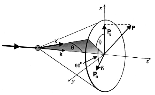
Figure 2.4: Vectors and angles in Mott scattering (from the Ref.[17]).

The differential cross section for the polarised electron is dependent not only on the angle of deflection $\theta$ but also on the azimuthal angle $\phi$

$$\frac{d\sigma}{d\Omega}(\theta,\phi)=I(\theta)\left(1+S\left(\theta\right)\vec{P}\cdot\hat{n}\right)=I(\theta)\left(1+S\left(\theta\right)P_{n}\sin\phi\right),$$ (2.19)

where $\hat{n}=\frac{\hat{n_{1}}\times\hat{n_{2}}}{\sin\theta}$ is the unit vector normal to the scattering plane, $\hat{n_{1}}$ and $\hat{n_{2}}$ are unit vectors in the direction of the electron motion, respectively, before and after scattering and $P_{n}$ is a component of $\vec{P}$ along $\hat{n}$. After the scattering, the electron polarisation is given by

$$\vec{P}^{\prime}=\frac{\left[P_{n}+S\left(\theta\right)\right]\hat{n}+T(\theta)\hat{n}\times[\vec{P}\times\hat{n}]+U(\theta)[\hat{n}\times\vec{P}]}{1+\vec{P}\cdot\hat{n}}.$$ (2.20)

The $S$, $T$ and $U$ functions has been calculated and tabularised for a variety of elements and energies by Sherman [12].

Chapter 3 Experiment

The $R$-correlation measurement is being performed at the Paul Scherrer Institute in Villigen on the polarised cold neutron beam line of the spallation source SINQ [2]. Fig. 3.1 shows the layout of the line and demonstrates where both the polarisation and focusing of the beam take place.

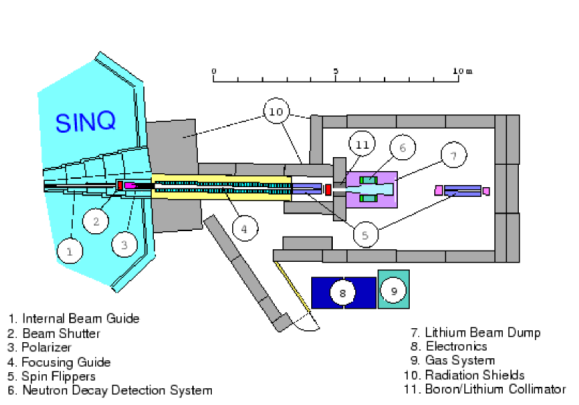
Figure 3.1: The spallation source SINQ with the polarised cold neutron beam line.

3.1 The main principle

According to section 2.1, a measurement of the electron polarisation component, which is perpendicular to the plane spanned by the spin of the decaying neutron and the electron momentum, will provide an estimation of the $\beta$ decay $R$-correlation parameter and, if the value was different than zero, would discover time reversal symmetry violating processes.

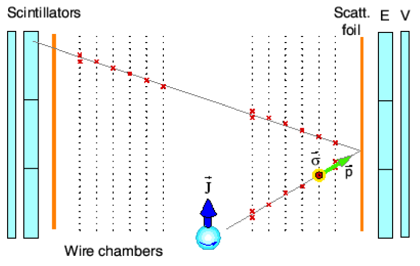
Figure 3.2: The principle of the measurement. The picture shows so called V-Track, which is the type of event desired for the transversal polarisation component determination.

The main principle of the measurement is shown in Fig. 3.2. An electron from the decay of a neutron with specified polarisation traverse the wire chamber detector. Afterwards, it scatters on the analysing foil covered with a layer of lead. Note, that the angle of scattering depends on the electron polarisation (Eq. 2.19). Deflected electrons traverse back the whole setup, including both wire chambers, the second Pb foil and, finally, hit the scintillator, where the remaining energy is left. Electron tracks from wire chambers provide possibility of reconstruction the emission and Mott scattering angles, which, together with the known neutron beam polarisation, is sufficient to obtain the $R$ parameter. In addition, the energy measurement from scintillators serves for distinguishing the signal from background, generated mostly by high energy electrons coming from neutron captures in surrounding.

The measurements are done for both neutron spin orientations (“up” and “down”), which helps to cancel out some systematic effects related to the setup geometry and to control better the remaining ones. Moreover, another important feature of this experimental configuration is to be used for the same purpose. It is clear that from the scattering angles one can acquire information on both transversal components of the electron polarisation, because for both of them the experimental technique is exactly the same and both can be measured simultaneously. Thus, the $N$-correlation parameter can be extracted from the data, as well as the $R$ parameter. Since the value of $N$ is well known (see Eq. 2.3), the comparison with the measured value will serve as an important clue to systematic errors limiting the experimental accuracy. Therefore, the behaviour of both electron polarisation components will be studied in the simulation.

3.2 Experimental setup

The collimated beam of cold neutrons enters the decay chamber filled with helium and covered with a special material enriched with ⁶Li. Both these elements were chosen to reduce the background, because helium has zero cross section for neutron capture and is easy to use and ⁶Li, which in contrary absorbs neutrons very well, does not in effect emit secondary $\gamma$ rays, which could convert to electrons in detector materials. In the lithium cover,

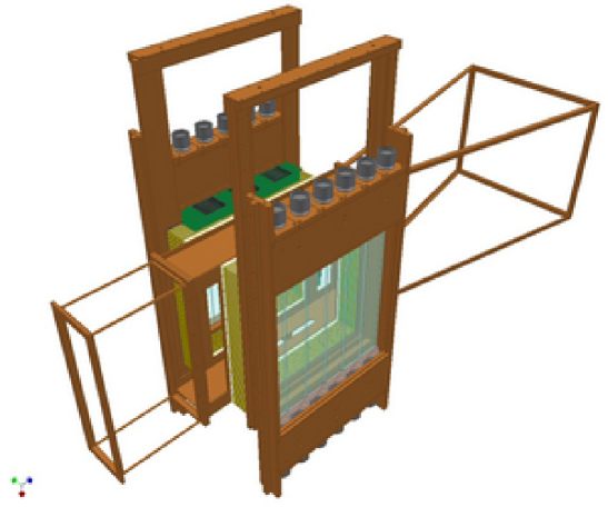
Figure 3.3: The helium box with MWPC detectors and hodoscopes.

on the sides of the decay chamber there are only two mylar windows separating MWPC (MultiWire Proportional Chamber) detectors from decay volume. The MWPC chambers are filled with a gas mixture of helium, methylal and isobutan, in proportion optimised for the best efficiency and stable operation. The analysing Pb foil is placed behind the next mylar window, in a small helium filled box. In this case, helium is meant to protect the foil from oxidising and is optimal with respect to energy loss ans multiple scattering. The last elements of the setup are two systems of position sensitive scintillators.

Chapter 4 Simulation

The comprehensive Monte Carlo simulation of the $R$-correlation experiment has been created by our group since the year 2001 and has already been useful for various purposes. Its present version is the sum of individual efforts made by few developers and contains all functionality from few recent versions like:

• EnergyLoss program for energy calibration,

• Sim used for the investigation of neutron background.

The first release of the code and its main part, including extended Geant4 classes for neutron capture, has been written by J. Pulut. E. Stephan has implemented the first version of the Mott scattering subroutine and the code for generation of the artificial wire chamber response.

So far the simulation has been useful for the energy calibration purposes and for the optimisation of the experimental setup geometry and materials. Now, with the use of new polarised dependent parts, it can be employed for the analysis of systematic effects. This chapter describes selected features of the simulation with the stress laid on the polarisation transport.

4.1 The Geant4 package

Geant4 (GEometry ANd Tracking) is a widely used set of C++ libraries for simulating the passage of particles through matter, originating in the old Fortran based Geant3 version. It includes a complete range of functionality including tracking, geometry and physics models and provides tools necessary for implementing a whole experiment in a program. With the use of Monte Carlo techniques Geant4 step by step calculates a particle energy losses, direction changes, creates secondary particles and simulates physical interactions. In general, the total cross section for the various relevant processes is used to select the process that will take place and when it is done, appropriate differential cross sections are used to calculate the kinematics. However, no electron polarisation sensitivity is included in the code. The details and further references can be found in the recent paper of the Geant4 project [22] and on the homepage [21].

4.2 Geometry

The whole geometry of the experimental apparatus and the neutron beam implemented in the simulation is based on its previous version (comprehensively described in Ref. [25]), updated for the new setup. It has been written in a flexible way, therefore, if needed, the user can easily modify materials and sizes of chosen setup elements or change the distances between them. All the parameters are available in the macro file geom.g4mac presented in appendices and in the source files src/GeometryConstans.icc and src/DetectorMaterials.icc . Of course, modification of the source files requires subsequent recompilation of the program. Fig. 4.1 demonstrates the implemented geometry and its details.

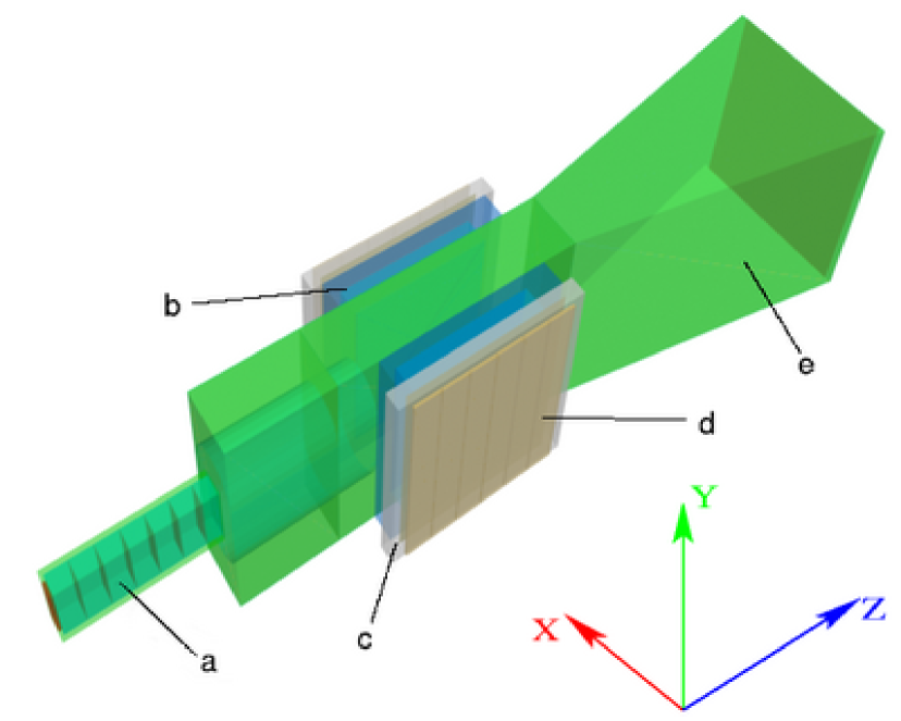
Figure 4.1: The geometry implemented in the simulation: a) the collimator, b) the proportional chamber, c) the helium box with the analysing lead foil, d) scintillators, e) the decay chamber. Directions of axes of the main reference system are shown as well. Please note that its origin is located in the middle of the decay chamber, between the wire chambers.

4.3 Polarisation transport

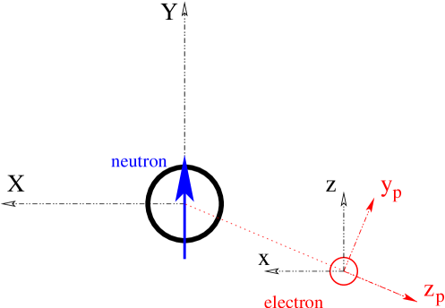
Figure 4.2: The main reference frame $\{X,Y,Z\}$ and both frames moving with the electron. $\{x_{p},y_{p},z_{p}\}$ denotes the particle frame.

The electron polarisation $\vec{\sigma}$, sampled as described in section 4.3.1, is given relative to a right-handed frame moving with the particle. However, the bookkeeping of all polarisation changes of a particular electron is performed in a coordinate system with the $z$ axis in the direction of motion, in the frame called the particle basis. Both frames are linked to each other through a simple rotation, given by a matrix similar to that of Eq. 2.15 (see Fig.4.2). The full definition of the particle basis $\{x_{p},y_{p},z_{p}\}$ and its relation to the laboratory reference system $\{X,Y,Z\}$ (see Fig. 4.1) is as follows:

• $z_{p}$ is in the direction of particle motion $\vec{v}=(v_{1},v_{2},v_{3})$, $\vec{v}$ is normalised

• $x_{p}$ is parallel to $XZ$ plane

• $Y$ is parallel to $y_{p}z_{p}$ plane.

The particle basis definition can be expressed using the formulae

$$\hat{x}_{p} = (\cos\phi,0,-\sin\phi),$$

$$\hat{y}_{p} = (-\sin\phi\sin\theta,\cos\theta,-\cos\phi\sin\theta),$$ (4.1)

$$\hat{z}_{p} = (v_{1},v_{2},v_{3}),$$

where

$$\sin\phi = \frac{v_{1}}{\sqrt{v_{1}^{2}+v_{3}^{2}}},$$

$$\cos\phi = \frac{v_{3}}{\sqrt{v_{1}^{2}+v_{3}^{2}}},$$

$$\sin\theta = \frac{v_{2}}{\sqrt{v_{1}^{2}+v_{2}^{2}+v_{3}^{2}}},$$

$$\cos\theta = \frac{\sqrt{v_{1}^{2}+v_{3}^{2}}}{\sqrt{v_{1}^{2}+v_{2}^{2}+v_{3}^{2}}}.$$

4.3.1 Electrons from $\beta^{-}$ decay

The first step of the simulation is the generation of electrons from $\beta^{-}$ decay with proper distributions of energy, momentum and polarisation. Although Geant4 provides possibility to generate decay of neutrons from the beam, it takes so much computational time, that for better efficiency the simulation starts from electrons. The neutron beam, however, together with the $\beta$ decay and neutron physics is implemented in the program and will be helpful in future for identifying main sources of background.

Electrons are uniformly created inside volume of given position and sizes corresponding to the real shape and spatial placement of the neutron beam. Their kinetic energy is sampled using the acceptance-rejection method and an approximated version of Eq. 2.1 (see Fig. 4.3)

$$W(E_{e})\propto p_{e}E_{e}(E_{max}-E_{e})^{2}.$$ (4.2)

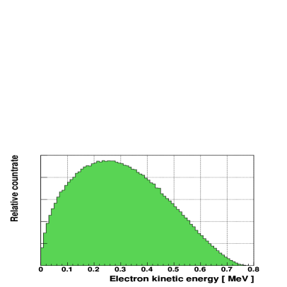
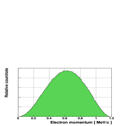
Figure 4.3: Simulated electron energy and momentum spectra (for 1 million events).

Finally, momentum and polarisation are generated from the probability distribution given by

$$W\propto\left[1+A\frac{\vec{\left<J\right>}\cdot\vec{p}_{e}}{E_{e}}+G\frac{\vec{\sigma}\cdot\vec{p}_{e}}{E_{e}}+N\vec{\sigma}\cdot\vec{\left<J\right>}+Q\frac{\vec{\sigma}\cdot\vec{p}_{e}}{E_{e}+m}\frac{\vec{\left<J\right>}\cdot\vec{p}_{e}}{E_{e}}+R\frac{\vec{\left<J\right>}\cdot\left(\vec{p}_{e}\times\vec{\sigma}\right)}{E_{e}}\right],$$ (4.3)

where the polarisation vector $\vec{\sigma}$ is normalised to unity. It is worth mentioning, that values of the decay parameters together with the mean beam polarisation $\vec{\left<J\right>}$ can be easily modified by the user (in the file run.mac). In addition to this, user defined limits on electron energy and emission angle can be applied which is necessary for optimisation purposes.

Figure 4.4 shows results of a simple test which was performed to check if assumed $A$ and $G$ values were reproduced in generated data. Comparing the probability distribution 4.3 with the fitted linear function, one can see that

$$A_{sim.}=\frac{E_{e}}{p_{e}\left<J\right>}\cdot p_{1}\mbox{\ \ \ and \ \ \ }G_{sim.}=\frac{E_{e}}{p_{e}}\cdot p_{1},$$

where $\left<J\right>=0.8973$ is the mean neutron beam polarisation and $\frac{E_{e}}{p_{e}}$ has to be averaged over the $\beta$ decay energy spectrum (what gives $\left<\frac{E_{e}}{p_{e}}\right>=1.368$). Finally, one obtains:

$$A_{sim.}=\frac{1.368}{0.8973}\cdot p_{1}=-0.118\pm 0.003\mbox{\ \ \ and \ \ \ }G_{sim.}=-0.999\pm 0.002,$$

which is in perfect agreement with the taken values: $A=-0.1162$ and $G=-1$.

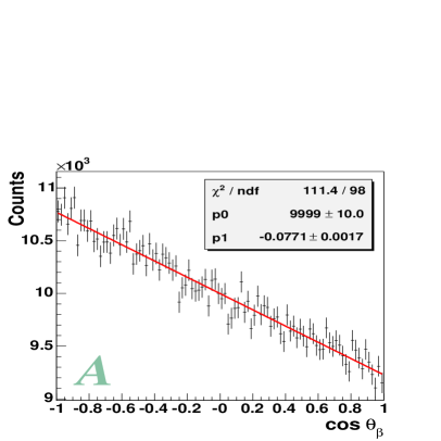
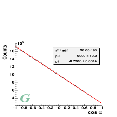
Figure 4.4: Simulated $A$ and $G$ decay asymmetries with fitted functions $y=p_{0}(1+p_{1}\cdot x)$. $\alpha$ is the angle between the electron momentum and polarisation. The number of generated electrons equals 1 million.

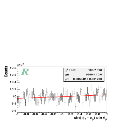
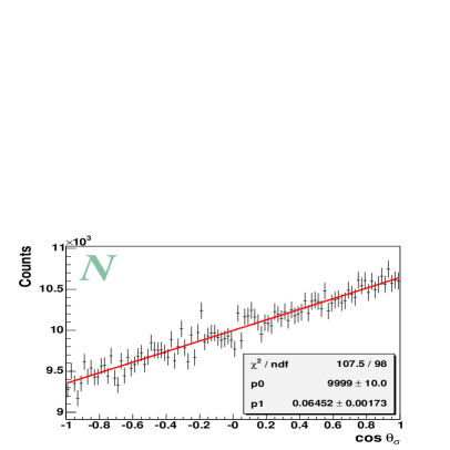
Figure 4.5: Simulated $R$ and $N$ coefficients. In both cases the fitted function is $y=p_{0}(1+p_{1}\cdot x)$.

Similar tests have been done for $N$ and $R$ asymmetries in the generated spin of the electron. Again, comparing the formula 4.3 with Fig. 4.5 after some calculations, one can obtain their values straight from the fit. The results are:

• for assumed $R=0.010$

  $$R_{sim.}=\frac{1.368}{\left<J\right>}\cdot p_{1}=0.008\pm 0.003,$$

• for assumed $N=-A\frac{m_{e}}{E_{e}}=0.076$

  $$N_{sim.}=\frac{1}{\left<J\right>}\cdot p_{1}=0.072\pm 0.002.$$

It is thus confirmed, that $\beta$ decay parameters are reproduced in generated data with fair accuracy.

4.3.2 Depolarisation

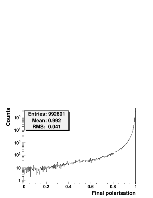
Figure 4.6: Depolarisation due to the Møller scattering

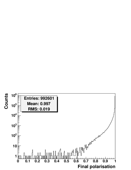
Figure 4.7: Depolarisation due to the multiple scattering

Figure 4.8: Depolarisation due to bremsstrahlung

Generated $\beta$ decay electrons traverse the experimental setup, namely the helium box and its mylar window, the proportional chamber filled with special gas mixture, another mylar window and the box containing the Pb foil, also filled with helium, where their transversal polarisation is to be analysed by Mott scattering. However, before reaching the analysing foil, electrons are partially depolarised through numerous interactions. This subsection contains some quantitative estimations of the polarisation loss based on the simulation results. In order to respect spin effects, Geant4 libraries have been extended using formulae from section 2.3. Before the actual results have been acquired, an especial effort had been made to check the reliability of the program and to verify the outcome with Ref. [10, section 4.3].

The figures below (4.6 – 4.8) show the depolarisation effects due to three implemented processes, separately (Geant4 gives possibility to “turn off” chosen physical processes). One million fully transversely polarised electrons have been shot from the point exactly in the middle of the helium box with momentum vector perpendicular to the Pb foil surface and the kinetic energy set to 700  k eV . The polarisation vector in the particle frame was $\vec{P}=(1,0,0)$ in order to investigate behaviour of the polarisation component strictly related to the $R$-correlation. The “final polarisation” on the pictures is the $\vec{P}_{x}$ component at the surface of the analysing foil, after the transportation through the whole setup. As it was expected, ionisation is the dominant process and the least change is caused by bremsstrahlung.

4.3.3 Mott scattering in the analyzing Pb foil

After crossing the proportional chamber, a partially depolarised electron can hit the analyzing foil covered with a layer of Pb, where it is scattered (as described in section 2.3.4). The formula 2.19, which governs this process, can be rewritten in a form

$$\frac{d\sigma}{d\Omega}(\theta,\phi)=I(\theta)\left[1+S\left(\theta\right)\left(P_{y}\cos\phi-P_{x}\sin\phi\right)\right],$$ (4.4)

which makes the dependence on the transversal polarisation component more obvious. As it was already mentioned, Geant4 does not contain any electron polarisation dependent processes, therefore to include the Mott scattering some extensions of the code have been done. The most important steps of the implemented routine are:

1. Functions $I$ and $S$ are loaded from the file (see Fig. 4.9).

2. As soon as an electron reaches the surface of the analyzing foil, the Geant4 tracking engine is stopped.

3. An exact point of the scattering inside the foil is generated from the uniform distribution.

4. The energy loss between the foil border and the scattering point is calculated using the database [24] and subtracted from the electron energy.

5. The new particle momentum is generated from the formula 4.4. If needed, the values of functions $I$ and $S$ are linearly interpolated.

6. The energy loss between the scattering point and the foil border is calculated and subtracted.

7. The new particle momentum and energy are passed to the Geant4 tracking engine, which is started again.

And here appears an important issue. The formula 4.4 is valid for the scattering on a single nuclei, what corresponds to the exact point of the scattering which is sampled in the third step of the routine. However, the electron in the foil can be also scattered two or more times, what cannot be neglected, even though for the foil thickness used in the experiment the single scattering is still more probable (the thicker is the Pb layer, the more probable is double or multiple scattering). The solution of this problem are, calculated for a given foil thickness, effective functions $I_{\mbox{\it eff}}(\theta)$ and $S_{\mbox{\it eff}}(\theta)$ which already contain multiple scattering effects and ought to be used instead of the normal cross section and analysing power. Both effective functions have been calculated by E. Stephan [4] with a dedicated Monte Carlo simulation based on Ref. [18] and are presented in Fig. 4.9.

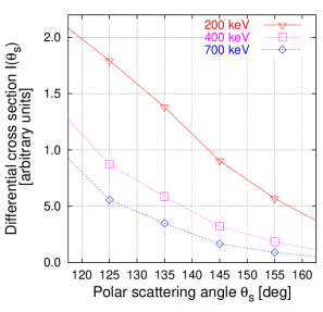
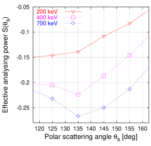
Figure 4.9: The differential cross section and the effective Sherman function used in the program. Both are results of an independent simulation performed by E. Stephan [4].

In order to check reliability of the Mott scattering routine a simple test have been prepared. Scattering of one million fully transversely polarized electrons with the polarisation vector

$$\vec{P}\equiv(P_{x},P_{y},P_{z})=\left(\frac{1}{\sqrt{5}},\frac{2}{\sqrt{5}},0\right)=(0.447,0.894,0)$$

and kinetic energy 700  k eV  have been simulated, resulting in angular distributions shown on Fig. 4.10. The scattering angle $\theta_{s}$ here, and for all other simulations, was restricted to the region 120 – 160 degrees, because for lower angles reflected electrons do not have a chance to hit the detector and for larger angles the cross section goes down rapidly. The cross section 4.4 averaged over the $\theta_{s}$ angle can be written as

$$\frac{d\sigma}{d\Omega}(\phi_{s})=\left<I\right>\left[1+\left<S\right>\sin\left(\phi_{s}+\delta\right)\right],$$ (4.5)

therefore full information about the transversal polarisation component is hidden in the phase shift $\delta$ and can be obtained from the fit (see Fig. 4.10). The results

$$P_{x}=-\cos\delta=0.454\pm 0.006 P_{y}=\sin\delta=0.891\pm 0.003,$$

are in a very good agreement with assumed values, what provides a satisfactory crosscheck.

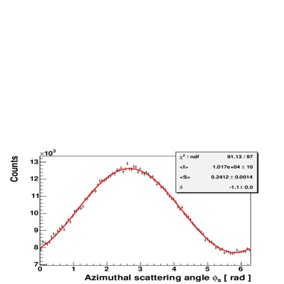
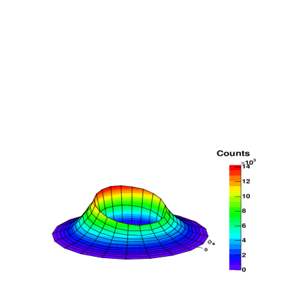
Figure 4.10: Test of the Mott scattering routine: distributions of the scattering angles. The function fitted to the $\phi_{s}$ distribution is $y=\left<I\right>[1+\left<S\right>\sin(\phi_{s}+\delta)]$.

One should be aware of several systematic errors that might be introduced here and could lower the accuracy of the simulation, especially when it will be used for prediction of the real measurement results:

• the effective functions $I_{\mbox{\it eff}}$ and $S_{\mbox{\it eff}}$ are model dependent and can contain some systematics caused by the generation method ([18]),

• because of the unavailability of proper data for ₈₂Pb, the analyzing power $S$ for ₈₀Hg has been used as the input for the $S_{\mbox{\it eff}}$ calculation,

• small additional deviations are caused by the linear interpolation of $I_{\mbox{\it eff}}$ and $S_{\mbox{\it eff}}$ values between the points of given energy and scattering angle,

• so far the electron depolarisation inside the Pb-foil, directly before the scattering has not been implemented.

Chapter 5 Systematic effects

After numerous careful tests of the program, described in the previous chapter, it finally could have been employed in realistic simulation of the whole experiment and its conditions. The results presented below required two days of calculations on a PC machine with a fast CPU. It was enough to reach the expected statistics of the planned experiment, namely, over one million events (V-Tracks). Due to the significant differences in cross sections and analysing powers, the data analysis was performed separately for three electron energy intervals:

• 200 k eV  – 400 k eV ,

• 400 k eV  – 600 k eV ,

• 600 k eV  – 800 k eV .

Electrons with energies below 200  k eV  were not generated, since the threshold of our apparatus is expected to be around this value. For optimisation reasons, after dedicated tests, some cuts have been also applied on electron generation angles:

• the polar angle: $\theta_{\beta}\in(15\mathrm{\SIUnitSymbolDegree},165\mathrm{\SIUnitSymbolDegree})$,

• the azimuthal angle: $\phi_{\beta}\in(20\mathrm{\SIUnitSymbolDegree},160\mathrm{\SIUnitSymbolDegree})$.

Moreover, the Mott scattering angle $\theta_{s}$ was restricted to a subset $(120\mathrm{\SIUnitSymbolDegree},160\mathrm{\SIUnitSymbolDegree})$. The motivation is clear, on the one hand side, there is no chance to detect in the opposite chamber an electron scattered with $\theta_{s}<120\mathrm{\SIUnitSymbolDegree}$, on the other hand for the scattering angles over $160\mathrm{\SIUnitSymbolDegree}$ electron tracks before and after scattering are not distinguished by the wire chamber.

5.1 Data analysis

First, it is necessary to describe the general concept of the data analysis. For each Mott scattering event (V-Track ) the simulation saves to a file the data specified below:

• initial momentum direction,

• momentum at the Pb foil surface, before the scattering,

• momentum after scattering,

• initial polarisation,

• polarisation at the Pb foil surface, before the scattering,

• the initial electron position,

• the scattering point position,

• final position at the scintillator border,

• initial kinetic energy,

• final kinetic energy,

• random deviation from the final kinetic energy (to simulate the effect of the finite energy resolution),

• artificially generated response of electrodes from the wire chambers.

The raw data files, containing values in the ASCII format, are later converted with the extended version of the NPRun[5] analysis program to binary *.root files. During this process a few important parts of the actual analysis are done, including the reconstruction of V-Tracks from the artificial wire chamber data. Afterwards one can work directly on the binary files, using the ROOT [27] environment and macros, created especially for that purpose. At this point, the analysis is done separately for momenta and positions reconstructed from artificial tracks and separately for the “real” values, taken straight from the simulation.

To obtain values of $R$ and $N$ coefficients from the simulated data, one has to know the intensity distribution of the azimuthal scattering angle $\phi_{s}$, which can be used to calculate mean values of the transversal polarisation components, just as it was shown in section 4.3.3. Both scattering angles can be calculated from momentum directions before and after scattering, transformed to the incoming particle frame (see section 4.3). The Fig. 5.1 shows the distribution of scattering angles for over 200000 V-Tracks, generated from the beam polarised in the “up” direction. Its shape is mostly a consequence of acceptance of the the experimental setup and beam geometry and in this form cannot be used for determination of the electron spin direction. To achieve a distribution independent on the geometry, just like in the real experiment, one has to flip the beam polarisation and produce the same amount of data. In this case, the influence of the geometry is exactly the same, while the effects caused by the polarisation contribute to the $\phi_{s}$ distribution with the opposite sign (from equations 4.3 and 4.4). After subtracting both distributions and normalising the result to the total number of events, one gets the final, geometry independent intensity distribution of Mott scattering angles for V-Tracks. The mean values of polarisation components can be now extracted from the fit.

5.2 Reconstruction of V-Tracks

Probably the most challenging problem in the analysis of data from the real experiment is the reconstruction of electron tracks based on signals from the MWPC chambers. To avoid depolarisation and multiple scattering effects, the chambers are relatively thin (around 10 cm) and contain only 5 planes of electrodes. Each plane consists of one layer of anodes (horizontal wires) and two layers of cathodes (vertical wires).

The reconstruction algorithm, implemented in the NPRun program is in its advanced development phase and still requires some tests, while the simulation provides the only possibility to compare “real” tracks with the reconstructed ones and to check the reconstruction efficiency. Therefore, some qualitative comparisons have been done.

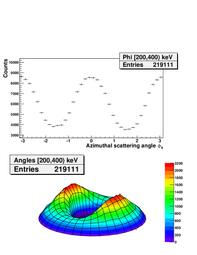
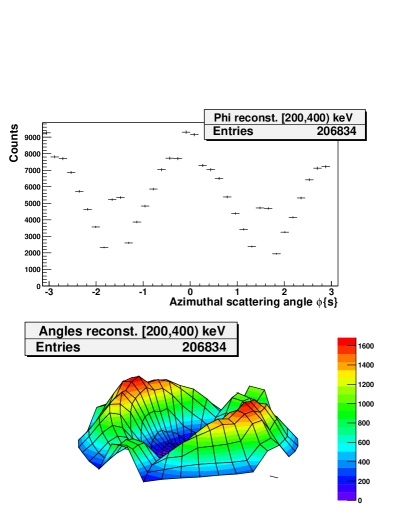
Figure 5.1: The comparison of the distribution of real scattering angles $\phi_{s}$ (pictures on the left) with the reconstructed ones (on the right).

As we can see in Fig. 5.1, the reconstruction works fine, with very high efficiency, however, for the angles $\phi_{s}=0,\pm\frac{\pi}{2},\pm\pi$ there is a large difference. The missing reconstruction efficiency in that specific geometry is due to MWPC wire layout feature. The reconstruction of V-Tracks has to be done separately for two projections (for anodes and cathodes). The problem arises for V-Tracks which lay either in the cathodes or in the anodes plane. Since they can be fully reconstructed in only one projection, ambiguities can appear. The scattering angle values $\phi_{s}=0,\pm\frac{\pi}{2},\pm\pi$ correspond exactly to these events. The version of the algorithm tested in this case reconstructs as much of these type of V-Tracks as possible which results in many misidentified tracks.

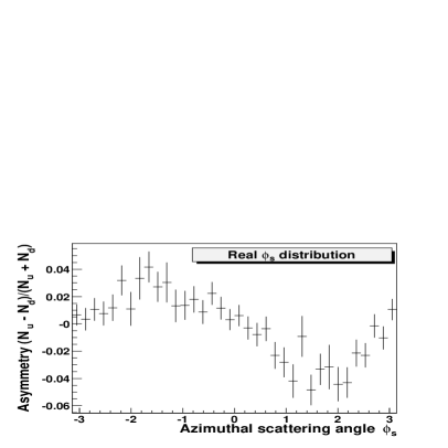
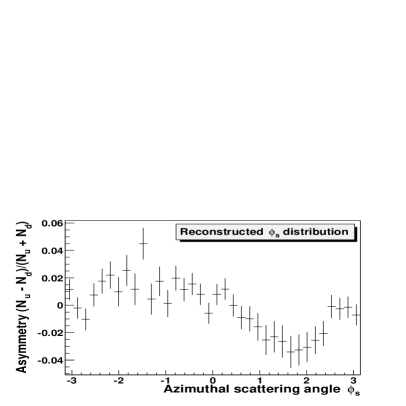
Figure 5.2: The comparison of the real scattering angles (picture on the left) with the reconstructed ones (on the right) after the subtraction of data corresponding to opposite beam polarisations.

At the final stage of the analysis the effect cancels out (on the cost of lower statistics) and the ultimate result is satisfactory (Fig. 5.2). It should be added here, that in reality the efficiency of the reconstruction algorithm is much lower, due to the noisy signal from the chambers caused by various sources of background. The algorithm for the artificial chamber signal generation includes the optional noise generation, but in this case it has not been used.

5.3 False R-correlation

Although, the false contribution to the $R$ coefficient caused by the neutron decay asymmetry was one of the expected systematic effects (a similar effect appeared in the $R$ measurement for ⁸Li [15]), its nature have been understood and the magnitude have been estimated very recently, by means of this simulation. Figures 5.3 and 5.4 explain the source of the effect. Let’s consider the situation when the beam is polarised in the “up” direction. For simplicity, the dependency on the electron polarisation is not taken into account. Because of the neutron decay asymmetry (nonzero $A$ coefficient), more electrons are emitted “down”, in the direction opposite to the beam polarisation.

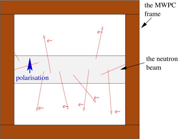
Figure 5.3: The neutron beam as seen from the position at the analysing Pb foil.

In the case of the electrons emitted “up”, the scattering angle value $\phi_{s}=-\frac{\pi}{2}$ is less probable than $\frac{\pi}{2}$, since only the backscattered particles are accepted by the simulation. Knowing that in the program $\theta_{s}\in(120\mathrm{\SIUnitSymbolDegree},160\mathrm{\SIUnitSymbolDegree})$, one can see that the effect starts to appear for the angle between the incoming electron momentum and the scattering foil plane $\alpha<60\mathrm{\SIUnitSymbolDegree}$. In contrary to this, for the much larger number of particles emitted in the direction “down”, the effect is opposite and $\phi_{s}=-\frac{\pi}{2}$ is more probable than $\frac{\pi}{2}$.

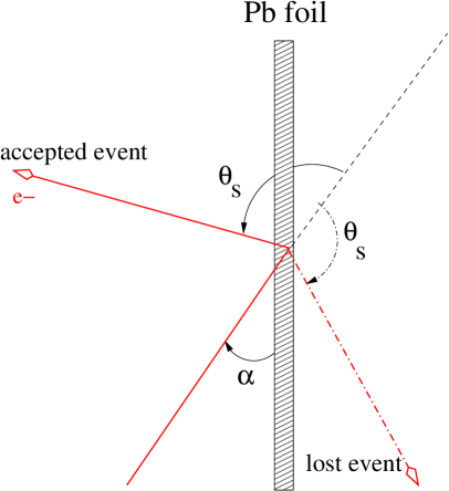
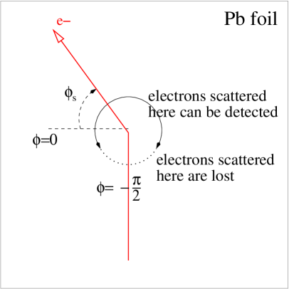
Figure 5.4: The principle of the systematic effect. For electrons emitted in the direction “up” the scattering angle $\phi_{s}=-\frac{\pi}{2}$ is less probable than the angle $\frac{\pi}{2}.$

Of course, if the beam polarisation is flipped, the effect is reversed, therefore it cannot be canceled by subtraction of $\phi_{s}$ distributions measured for both beam polarisations. It results in the final sine-like angular distribution, with one maximum at $\phi_{s}=-\frac{\pi}{2}$ and one minimum at $\phi_{s}=\frac{\pi}{2}$ (see Fig. 5.5). As it was specified before, it is exactly the shape that one would expect for the nonzero $R$ coefficient. Therefore, it is necessary to examine this effect and estimate the induced false contribution to the measured $R$ coefficient.

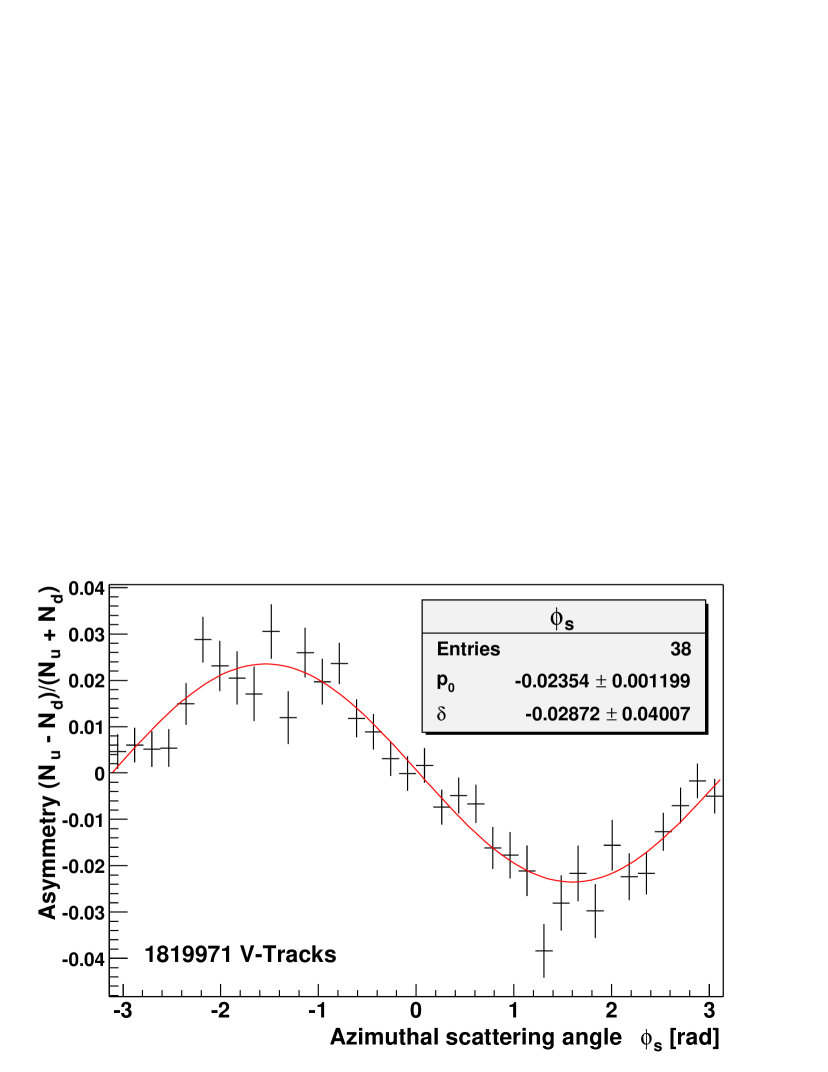
Figure 5.5: The false $R$ effect for the initial electron energy $E_{k}\in(200,782)\mathrm{k}\mathrm{eV}$. $N_{u}$ and $N_{d}$ denote the count rate for the “up” and “down” beam polarisation, respectively. The function $y=p_{0}\cdot\sin(\phi_{s}+\delta)$ has been fitted to data points.

A dedicated simulation have been performed for that purpose. In order to separate the effects induced by the $\beta$ decay asymmetry, all the coefficients except $A$ have been set to zero. The program has produced almost 2 million V-Tracks, half of them with the beam polarisation “up” and half with the opposite. The total result averaged over the electron kinetic energy $E_{k}>200\leavevmode\nobreak\ \mathrm{k}\mathrm{eV}$ and over all generation angles is presented in the Fig. 5.5. However, even more interesting are similar pictures for three distinct electron energy intervals (Fig. 5.6).

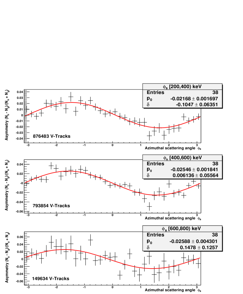
Figure 5.6: The false $R$ effect for three electron energy intervals. The function $y=p_{0}\cdot\sin(\phi_{s}+\delta)$ has been fitted to data points.

The amplitudes $p_{0}$ taken from the fit can be now used to calculate the false contribution to the average value of the transversal electron polarisation component. The intensity distributions are given by:

$$N_{u}(\phi_{s}) = \left<I\right>[1+\left<S\right>\sin(\phi_{s}+\delta)]=\left<I\right>[1+\left<S\right>(P_{y}\cos\phi_{s}-P_{x}\sin\phi_{s})],$$

$$N_{d}(\phi_{s}) = \left<I\right>[1+\left<S\right>(-P_{y}\cos\phi_{s}+P_{x}\sin\phi_{s})],$$

thus

$$\frac{N_{u}-N_{d}}{N_{u}+N_{d}}=\frac{2\left<I\right>\left<S\right>(P_{y}\cos\phi_{s}-P_{x}\sin\phi_{s})}{2\left<I\right>}=\left<S\right>\sin(\phi_{s}+\delta).$$

The average Sherman function values for specified energy ranges are:

$E_{k}[\mathrm{k}\mathrm{eV}]$	200 – 400	400 – 600	600 – 800
$\left<S\right>$	-0.15	-0.20	-0.23

and both transversal polarisation components:

$$P_{x}=-\frac{\cos\delta}{\left<S\right>}\cdot p_{0}, P_{y}=\frac{\sin\delta}{\left<S\right>}\cdot p_{0}.$$

The results are:

$E_{k}\ [\mathrm{k}\mathrm{eV}]$	200 – 400	400 – 600	600 – 800
$P_{x}$	$0.14\pm 0.01$	$0.13\pm 0.01$	$0.11\pm 0.02$
$P_{y}$	$0.00\pm 0.01$	$0.00\pm 0.01$	$0.00\pm 0.02$

Note, that the systematic error of the average $S$ has not been taken into account in the error estimation. An obvious conclusion from the above simple analysis is that the magnitude of the investigated systematic effect does not depend on the electron energy.

It should, however, depend on the electron emission angle as it was explained before. And that was the motivation of the last test that has been done. The false $R$ effect has been extracted from the data separately for different values of the polar angle between the normal to the scattering foil (the $x$ axis in the main reference system) and the initial electron momentum. In this case, events with all possible initial electron energies have been treated together and the average value of analysing power for the whole energy range 200 – 782  k eV  was assumed to be $\left<S\right>=-0.18$.

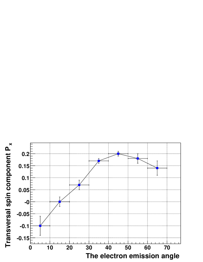
Figure 5.7: The false $R$ effect as a function of the electron emission angle.

The result is shown in the Fig. 5.7, one can see a clear dependency on the emission angle, what confirms that the nature of the systematic effect is well understood. For the emission angle below 50 ° its magnitude increases linearly (a similar situation like in Ref.[15]), later it starts to decrease. It can be explained by the fact that for the larger emission angles electrons may scatter on the MWPC frame, therefore their final angle at the foil can be dramatically changed. Accurate estimation of the false contribution to the $R$ coefficient is essential for the final systematic uncertainty of the whole measurement.

Chapter 6 Summary and conclusions

The main purpose of this thesis was the development of the comprehensive Monte Carlo simulation and the analysis of systematic uncertainties in the planned $R$-correlation coefficient measurement. The biggest effort was required to create and test the simulation program, based on the Geant4 package and to develop appropriate data analysis tools. In the first step, all previously written parts of software have been checked, debugged and unified in one application providing the full functionality. Furthermore, the new construction of the experimental apparatus had to be included replacing the old implementation. The most challenging part of the development phase was, however, the necessity of creating the code for the simulation of polarised electron processes and for the polarisation transport. So far, such an option has not been provided by the authors of Geant4 package.

Finally, the program has been used to search for systematic effects in the measurement. The first effect associated with the neutron $\beta$ decay asymmetry has been already recognized, explained and estimated. Due to the false contribution to the $R$ coefficient induced by this phenomena, it is essential to control it as well as it is possible. The Monte Carlo simulation provides the robust and powerful tool, which will serve for that purpose. Another important issue is the problem of the electron track reconstruction, which might introduce new systematic effects of different type. With artificial data, these contributions can be better controlled.

The search for other effects is in progress and definitely the program is going to be extensively used in future for the further measurement improvement and the data analysis.

Appendix A The macro run.mac

/gun/PositionRandom on
/gun/PositionRandomType linear

/gun/EnergyRandom on
/gun/EnergyRandomType raw
/gun/Decay on
/gun/particle e-

/gun/MomentumRandom on
/gun/AngleMinus 70 degree
/gun/AnglePlus 70 degree

# Neutron beam properties
/gun/XBeam 45. mm
/gun/YBeam 145. mm
/gun/XDiv 0.8 degree
/gun/YuDiv 0.9 degree
/gun/YdDiv 0.65 degree
/gun/range 1.1
/gun/neutron_polarization 0.8973
/gun/NeutronSpinRandom on

# Neutron beta decay parameters
/gun/A 0.0
/gun/R 0.0
/gun/N 0.0

/chamber/threshold_v .4
/chamber/threshold_h .8
/chamber/sjit_v 10.
/chamber/sjit_h 10.
/chamber/rnoise_level_v 0.
/chamber/rnoise_level_h 0.
/chamber/effiplane 0.95

/run/beamOn 1
#/run/beamOn 50000000

Appendix B The macro geom.g4mac

#Titan Foil
#/mydet/boron_box/ti_foil_thickness Ψ5.393 micrometer
# full thickness of the Ti foil (for energy loss simulation)
/mydet/boron_box/ti_foil_thickness Ψ0.0 micrometer

# Boron box
/mydet/boron_box/bigger_x ΨΨ700. ΨmmΨ# boron box width (with at the end of the box)
/mydet/boron_box/smaller_x ΨΨ214. ΨmmΨ# boron box width (the central part)
/mydet/boron_box/height ΨΨ625. ΨmmΨ# height of the b.b.
/mydet/boron_box/length ΨΨ2533.5 ΨmmΨ# total b.b. length
/mydet/boron_box/begin_length ΨΨ360. ΨmmΨ# length of the beginning of the b.b.
/mydet/boron_box/end_length ΨΨ1278.5ΨmmΨ# length of the ending of the b.b.
/mydet/boron_box/border ΨΨ1.25 ΨmmΨ# total b.b. border thickness
/mydet/boron_box/mid_border 1.2 ΨmmΨ# thickness of the inner layer of the border

/mydet/boron_box/window/height 500. mmΨ# height of b.b. windows
/mydet/boron_box/window/width 500. mmΨ# width of b.b. windows
                                    # window placement:
/mydet/boron_box/window/y_pos 0. cmΨ# - height
#(relative to the geometrical center of the b.b.)
/mydet/boron_box/window/z_pos 810. mmΨ# - z-axis position (along the beam)

# Dump
/mydet/boron_box/dump/width 650. mm Ψ# beam dump sizes
/mydet/boron_box/dump/height 622.5 mm Ψ#
/mydet/boron_box/dump/thickness 3.6 mm Ψ# and its placement
#/mydet/boron_box/dump/position 2530. mm # along the beam line

# MWPC
/mydet/mwpc/height ΨΨ625.Ψmm # MWPC sizes:
/mydet/mwpc/length ΨΨ625.Ψmm #Ψ
/mydet/mwpc/thickness ΨΨ91. Ψmm #
/mydet/mwpc/zposition_left      810. Ψmm # rel. to the beam: left chamber
/mydet/mwpc/yposition_left      0. Ψcm #
/mydet/mwpc/zposition_right     810. Ψmm # right chamber
/mydet/mwpc/yposition_right     0. Ψcm #

# Wire chamber
/mydet/mwpc/inside_height ΨΨ500. Ψmm # chamber sizes (inside the MWPC)
/mydet/mwpc/inside_length ΨΨ500.  Ψmm #
/mydet/mwpc/anode_spacing ΨΨ5. Ψmm # distance between anodes
/mydet/mwpc/dist_anode_cathode ΨΨ4. Ψmm # distance between anode and cathode planes
/mydet/mwpc/cathode_spacing ΨΨ2.5 Ψmm # distance between cathodes
/mydet/mwpc/anode_plane_spacing Ψ16. Ψmm # distance between anode planes
/mydet/mwpc/anode_diameter   25. micrometer        # wire diameter (anodes)
/mydet/mwpc/cathode_diameter 25. micrometer        # wire diameter (cathodes)
/mydet/mwpc/dist_entr_anode Ψ        12. Ψmm # distance between the chamber
# entrance and the nearest anode
/mydet/mwpc/anode_planes ΨΨ0          # total planes number

/mydet/mwpc/material/isobutane  Ψ10.   Ψ   # gas mixture: -percent of isobutane
/mydet/mwpc/material/methylal   Ψ6.  Ψ   #  Ψ      -percent of methylal

# Scintillators
/mydet/scintillator/height 60. cm Ψ# scintillator sizes
/mydet/scintillator/width 10. cm Ψ#
/mydet/scintillator/thickness 10. mm Ψ#
/mydet/scintillator/spacing 1. mm Ψ# scintillator spacing
/mydet/scintillator/number 6ΨΨ# number of scintilators

# Golden (lead ?) foil
/mydet/foil/width 60. cm Ψ# foil sizes
/mydet/foil/height 60. cm Ψ#
/mydet/foil/foil inΨΨ# "in" or "out" (with and without the foil)

# Distances
#/mydet/to_left_mwpcΨ0. mm ΨΨ# between b.b. surface and the left MWPC window
/mydet/to_right_mwpc Ψ0. mm ΨΨ# between b.b. surface and the right MWPC window
/mydet/to_scintillator Ψ6.6Ψcm Ψ# between MWPC’s and hodoscopes
/mydet/to_golden_foil Ψ3.2Ψcm Ψ# betweem MWPC’s and the lead foil

# Nose (Collimator)  --------------------------------------  only rough values
/mydet/nose/bars_number 6Ψ# number of barriers inside the collimator
/mydet/nose/to_barrier 50. mm Ψ# distance between the nose ending and
# the first barrier
/mydet/nose/border 11.2 mmΨ# total thickness of the "nose" border
/mydet/nose/mid_border 1.2 mmΨ# thicknes of the inner layer of the border

References

- [1] K. Bodek, T. Boehm, D. Conti, N. Danneberg, W. Fetscher, C. Hilbes, M. Janousch, St. Kistryn, K. Köhler, J. Lang, M. Markiewicz, J. Sromicki, J. Zejma, Nucl. Instr. and Meth. A 473, 326-334 (2001).
- [2] K. Bodek, P. Böni, C. Hilbes, J. Lang, M. Lasakov, M. Lüthy, S. Kistryn, M. Markiewicz, E. Medviediev, V. Pusenkov, A. Schebetov, A. Serebrov, J. Sromicki, A. Vasiliev, Neutron News 3, 29 (2000).
- [3] G. Ban, M. Beck, A. Białek, K. Bodek, T. Bryś, G. Frei, C. Hilbes, G. Kühne, P. Gorel, K. Kirch, St. Kistryn, A. Kozela, M. Kuźniak, A. Lindroth, O. Naviliat-Cuncic, J. Pulut, N. Severijns, E. Stephan, J. Zejma FUNSPIN Polarized Cold-Neutron Beam at PSI, submitted to Elsevier Science (June 2004).
- [4] E. Stephan, private communication.
- [5] C.Hilbes, A.Kozela, J.Pulut, private communication.
- [6] J.D. Jackson, S.B. Treiman, H.W. Wyld, Phys. Rev. 106, 517 (1957).
- [7] T.D. Lee, C.N. Yang, Phys. Rev. 104, 254 (1956).
- [8] H.A. Tolhoek, Electron polarization, theory and experiment, Rev. Mod. Phys. 28, 277-298 (1956).
- [9] W.H. McMaster, Matrix representation of polarization, Rev. Mod. Phys. 33(1), 8-29 (1961).
-
[10]
J.M. Hoogduin, Electron, positron and photon polarimetry,
University Library Groningen (1997),
http://www.ub.rug.nl/eldoc/dis/science/j.m.hoogduin/. - [11] H. Davies, H.A. Bethe, L.C. Maximon, Theory of Bremsstrahlung and Pair Production. II. Integral Cross Section for Pair Production, Phys. Rev. 93(4), 788-795 (1954).
- [12] N. Sherman, Coulomb scattering of Relativistic Electrons by a Point Nuclei, Phys. Rev. 103(6), 1601 (1956).
- [13] S.M. Seltzer, M.J. Berger, Nucl. Instr. and Meth. B 12, 95 (1985).
- [14] Y-S. Tsai, Rev. Mod. Phys. 49, 421 (1977).
- [15] J. Sromicki et al., Study of time reversal violation in decay of polarized , Phys. Rev. C 53, 932-955 (1996).
- [16] P. Stehle, Calculation of electron-electron scattering, Phys. Rev. 110(6), 1458-1460 (1958).
- [17] M.A. Khakoo et al., Monte Carlo studies of Mott scattering asymmetries from gold foils, Phys. Rev. A 64, 052713 (2001).
- [18] V. Hnizdo, Plural and multiple Mott scattering by Monte Carlo method, Nucl. Instr. and Meth. 109, 503-507 (1973).
- [19] H.W. Lewis, Phys. Rev. 78, 526 (1950).
- [20] K. Hagiwara et al. (Particle Data Group), Phys. Rev. D 66, 010001 (2002).
-
[21]
Geant4 Home Page,
http://geant4.web.cern.ch/geant4. - [22] S. Agostinelli et al., Nucl. Instr. and Meth. A 506, 250-303 (2003).
-
[23]
Physics Reference Manual, Geant4 Users’ Documents,Version: Geant4 6.1 (March 2004),
http://wwwasd.web.cern.ch/wwwasd/geant4/G4UsersDocuments/Overview/html/. -
[24]
M.J. Berger, J.S. Coursey, M.A. Zucker, The ESTAR database v1.2,
http://physics.nist.gov/PhysRefData/Star/Text/contents.html. -
[25]
M. Kuźniak, Geometria detektora do symulacji komputerowej eksperymentu, Praca roczna 2001
http://fremont.republika.pl/fizyka/manual.ps. - [26] The nTRV Homepage, http://www.if.uj.edu.pl/ZFJ/nTRV.
- [27] The ROOT System Homepage, http://root.cern.ch.