Extended sudden approximation model for high-energy nucleon removal reactions

Abstract

A model based on the sudden approximation has been developed to describe high energy single nucleon removal reactions. Within this approach, which takes as its starting point the formalism of Hansen [1], the nucleon-removal cross section and the full 3-dimensional momentum distributions of the core fragments including absorption, diffraction, Coulomb and nuclear-Coulomb interference amplitudes, have been calculated. The Coulomb breakup has been treated to all orders for the dipole interaction. The model has been compared to experimental data for a range of light, neutron-rich psd-shell nuclei. Good agreement was found for both the inclusive cross sections and momentum distributions. In the case of ¹⁷C, comparison is also made with the results of calculations using the transfer-to-the-continuum model. The calculated 3-dimensional momentum distributions exhibit longitudinal and transverse momentum components that are strongly coupled by the reaction for $s$-wave states, whilst no such effect is apparent for $d$-waves. Incomplete detection of transverse momenta arising from limited experimental acceptances thus leads to a narrowing of the longitudinal distributions for nuclei with significant $s$-wave valence neutron configurations, as confirmed by the data. Asymmetries in the longitudinal momentum distributions attributed to diffractive dissociation are also explored.

I Introduction

The breakup of light exotic nuclei has proven over the last decade to be a particularly useful tool to study the structure of nuclei far from stability (see, for example, [2, 3]). In the specific case of well developed single-nucleon halo nuclei, such as ¹¹Be, much insight has been gained into the reaction process. Early work by Serber [4], Glauber [5] and Dancoff [6] (later refined by Faldt [7]), investigating high-energy deuteron breakup, demonstrated that the relevant mechanisms governing the reaction are stripping, diffraction and Coulomb dissociation. More recently these concepts have been adapted by Hansen to describe quantitatively the breakup of the one-neutron halo nucleus ¹¹Be [1, 8].

The basic premise of the model – dubbed the “sudden approximation” – is that the reaction proceeds by the instantaneous removal of a nucleon from the projectile without disturbing the remaining nucleons. This approximation is justified for reaction times much shorter than the characteristic time for the motion of the nucleons within the projectile. A number of assumptions make the calculations particularly simple whilst retaining the essential physical concepts: (i) the incident energy is high enough so that the intrinsic velocity of the valence nucleon is much smaller than the projectile velocity; (ii) the projectile and the fragment follow straight-line trajectories; (iii) final-state interactions are neglected; (iv) the tail of the valence nucleon wave function is well developed, so reactions involving the valence particle are essentially surface peaked; (v) the target nucleus can be described by a “black disk”, so that the nucleon scattered or absorbed by the target is not observed; (vi) there is only one bound state of the system, the ground state (the completeness of the wave functions thus allows the transition probabilities to the continuum to be calculated via sum rules); and (vii) only the dominant part (the transverse component) of the momentum transfer generated by the Coulomb field of the target is considered.

These asumptions are well satisfied in the case of reactions involving a well developed one-neutron halo nucleus such as ¹¹Be. In this case, where the $rms$ radius of the halo is some three times larger than that of the core, only the asymptotic part of the halo wave function was required (see (iv)) [1, 9]. This leads to analytical formulae for the transition probabilities in impact parameter space and the longitudinal momentum distributions. In particular, in evaluating the longitudinal momentum distributions, Hansen proposed that to a good approximation the wave function of the valence nucleon could be evaluated at the center of the target [9]. This approximation leads to the interesting result that in the limit of very small binding energies the breakup cross section factorizes into the free neutron-target cross section and the probability that the neutron is at the center of the target with a longitudinal momentum close to the incident momentum per nucleon. Thus, the model is intimately related to the spectator model of Hussein and McVoy [10]. Whilst this approximation is well suited for the evaluation of longitudinal momentum distributions, it leads to a strong cutoff in the perpendicular momenta and is, therefore, less appropriate for the evaluation of the momentum distributions in a plane perpendicular to the beam direction.

In a recent report, Barranco and Vigezzi [11] have employed a similar approximation and obtained the result that the width of the perpendicular momentum distribution essentially reflects the target size and is more or less independent of the structure of the projectile ground-state wave function. This conclusion does not agree with recent work we have undertaken whereby the transverse momentum distributions were demonstrated to be sensitive to nuclear structure [12, 13]. The sudden approximation model requires a proper normalization of the various transition probabilities, and therefore cannot be extended easily to cases where the ground state is dominated by $p$ or $d$ waves. In such cases, for neutrons the asymptotic part of the radial wave function is given by Haenkel functions, which exhibit a strong singularity at the origin and the corresponding breakup probabilities cannot be defined properly. Clearly, in such a case, the transition probabilities should be defined in terms of realistic wave functions.

As discussed in our earlier papers [12, 13] and elsewhere [2, 14] single-nucleon removal reactions appear to be a powerful tool to probe structure far from stability. It is therefore highly desirable to test and compare various models of the reaction process in order that spectroscopic information may be extracted with confidence. In this spirit we have extended the sudden approximation model to deal with single-nucleon removal reactions where the ground state has an arbitrary structure for which the single-particle degrees of freedom can be disentangled. The model is conceptually simple and almost all observables may be calculated with a reasonable numerical effort even when realistic wave functions are used.

The paper is organized as follows. Sections II to V are devoted to the basic formalisms and development of the model. A comparison of the model calculations and experimental data for single-neutron removal is described in Section VI. For comparison the predictions of the transfer-to-the-continuum model [15, 16] for ¹⁷C are also given. The effects of finite detection acceptance are discussed in Section VII. Conclusions are drawn and summarized in Section VIII. Analytical formulae for various observables are provided in the Appendices.

II Basic Formalism

We assume that the ground state of the projectile $(J^{\pi})$ can be approximated by a superposition of configurations of the form $[I_{c}^{\pi}\otimes nlj]^{J^{\pi}}$, where $I_{c}^{\pi}$ denotes the core states and $nlj$ are the quantum numbers specifying the single-particle wave function of the valence nucleon. This is evaluated in a Woods-Saxon potential using the effective separation energy, $S^{eff}_{n}=S_{n}+E_{x}$ ($E_{x}$ being the excitation energy of the core state). Couplings of core states to the final state and dynamical excitation of core states in the reaction are neglected. In this approximation the reaction can populate a given core state only to the extent that there is a nonzero spectroscopic factor $C^{2}S(I^{\pi}_{c},nlj)$ in the projectile ground state. When more than one configuration contributes to a given core state, the total cross section for single-nucleon removal is written, following refs. [17, 18], as an incoherent superposition of single particle cross sections,

$$\sigma_{-1n}(I^{\pi}_{c})=\sum_{nlj}C^{2}S(I^{\pi}_{c},nlj)\;\sigma_{sp}(nlj,S^{eff}_{n})$$ (1)

The total inclusive single-nucleon removal cross section ($\sigma_{-1n}^{sudd}$) is then the sum over the cross sections to all core states. A similar relation holds for the momentum distributions. The term $\sigma_{sp}$ is the cross section for the removal of a nucleon from a single-particle state with total angular momentum $j$,

$$\psi_{jm}=R_{jl}(r)\sum_{m_{l},m_{s}}C^{l~{}~{}{{1}\over{2}}~{}~{}j}_{m_{l}m_{s}m}Y_{lm_{l}}(\hat{r})\chi_{{{1}\over{2}}m_{s}}(\sigma).$$ (2)

evaluated with the effective nucleon separation energy $S_{eff}$ defined above. We consider only spin independent transition operators and therefore all formulae are much simpler with the wave function,

$$\psi_{0}(\vec{r})=R_{l}(r)Y_{lm}(\hat{r}),$$ (3)

and the normalization,

$$\int d\vec{r}|\psi_{0}(\vec{r})|^{2}=1.$$ (4)

Certain cross sections may be expressed in a simpler form in a coordinate system traveling with the beam. The impact parameter with components in the direction connecting the centre of the core with that of the target is denoted by $\vec{b}$. Recoil effects are of the order $O(\frac{1}{A_{p}})$, where $A_{p}$ is the projectile mass number and are neglected here. The situation is illustrated in Fig. 1. After the interaction with the target a part of the wave function is removed. At this stage the specific form of the wound ($(w)$) is not important. The removed part of the wave function is then,

$$\delta\psi(\vec{r})=\left\{\begin{array}[]{ll}\psi_{0}(x,y,z)&\textrm{if}~{}(x,y,z)\in$(w)$\\ 0&\textrm{otherwise.}\\ \end{array}\right.$$

The complement ($\bar{\psi}$) is defined by the following orthogonal decomposition of the wave function,

$$\psi_{0}=\bar{\psi}+\delta\psi$$ (5)

$$\int d\vec{r}\bar{\psi}^{*}\delta\psi=\int d\vec{r}\bar{\psi}\delta\psi^{*}=0$$ (6)

If the nucleon is absorbed, the wave function of the system is localized to $\delta\psi$ at the instant of collision and this is then the state of the remaining core fragment. Consequently, the momentum distribution is given by the square of the Fourier transform of $\delta\psi$. The stripping (absorption) probability is given by the volume integral of the wound,

$$P_{a}(b)=\int d\vec{r}|\delta\psi|^{2}$$ (7)

As mentioned in ref. [1], “absorption” is defined here in the context of the black disk model. The wound complement is normalized as,

$$\int d\vec{r}|\bar{\psi}|^{2}=1-P_{a}$$ (8)

The wave function after collision with the target is approximated by,

$$\psi(\vec{r})=e^{i\vec{q}\vec{r}}(\psi_{0}-\delta\psi)=e^{i\vec{q}\vec{r}}\bar{\psi}$$ (9)

where $\vec{q}$ is the momentum transfer to the valence nucleon defined by Eq. (A.4) in Appendix A. The sudden transfer of a momentum $\vec{q}$ attaches a phase $e^{i\vec{q}\vec{r}}$ to the wave function. The physical meaning of the phase is clarified in Section V. This wave function has the normalization ,

$$\int d\vec{r}\psi^{*}(\vec{r})\psi(\vec{r})=\int d\vec{r}\bar{\psi}^{*}(\vec{r})\bar{\psi}(\vec{r})=1-P_{a}$$ (10)

Note that $\psi$ contains elastic as well as inelastic (breakup) states. The elastic content is given by the overlap with the ground state,

$$\gamma_{el}=\int d\vec{r}\psi\psi_{0}^{*}(\vec{r})$$ (11)

The wave function orthogonal to the ground state is,

$$\psi_{1}(\vec{r})=\psi(\vec{r})-\gamma_{el}\psi_{0}(\vec{r})$$ (12)

Now we are ready to construct the wave function for the decaying state ($\psi_{d}(\vec{r})$),

$$\psi_{d}(\vec{r})=\psi_{0}(\vec{r})-\delta\psi(\vec{r})-\gamma_{el}e^{-i\vec{q}\vec{r}}\psi_{0}(\vec{r})\equiv\bar{\psi}-\gamma_{el}e^{-i\vec{q}\vec{r}}\psi_{0}\equiv e^{-i\vec{q}\vec{r}}\psi_{1}(\vec{r})$$ (13)

As the state which is decaying contains only square integrable functions it is legitimate to speak about the norm of this wave function,

$$\int d\vec{r}|\psi_{d}(\vec{r})|^{2}=\int d\vec{r}|\psi_{1}(\vec{r})|^{2}=1-P_{a}-|\gamma_{el}|^{2}$$ (14)

Clearly, all information concerning the absorption of the valence nucleon is contained in the wave function of the wound ($\delta\psi$), whilst $\psi_{d}$ will furnish information on the elastic breakup. Let us calculate the Fourier transform of the decaying state,

$$\widetilde{\psi_{d}}(\vec{k})=\frac{1}{(2\pi)^{3/2}}\int d\vec{r}e^{-i\vec{k}\vec{r}}\psi_{d}(\vec{r})$$ (15)

The differential cross section in momentum space is given by,

$$\frac{d\sigma}{d\vec{k}}=\int 2\pi bdb|\widetilde{\psi_{d}}(\vec{k})|^{2}$$ (16)

and the total cross section by,

$$\sigma=\int 2\pi bdb\int d\vec{k}|\widetilde{\psi_{d}}(\vec{k})|^{2}=\int 2\pi bdb(1-P_{a}(b)-|\gamma_{el}(b)|^{2})$$ (17)

Now it is clear that the quantity,

$$P_{el}(b)=1-P_{a}(b)-|\gamma_{el}(b)|^{2}$$ (18)

should be interpreted as the probability in the impact parameter representation of the elastic breakup process. Relation (18) shows that the sudden approximation model accounts for stripping ($P_{a}$), elastic breakup or dissociation ($P_{el}$) and nuclear and Coulomb elastic scattering ($\gamma_{el}$). Other inelastic processes such as core absorption, simultaneous absorption of the valence neutron and the core [19] or “damped breakup” [20] are not included in this model. We also note that the closure relation (18) illustrates the need to use realistic wave functions in order to obtain properly normalized breakup probabilities.

III Breakup probabilities

In this section we discuss in detail the calculation of the breakup probabilities using two specific forms for the wound $(w)$. Using the same notations as in ref. [1] the planar cutoff is defined as,

$$(w):(x,y,z)\in\mathbf{R}^{3},~{}x\geq b_{1}=b-R_{t}$$

The second, the so called cylindrical wound is defined for arbitrary $z$ as,

$$(w):(x,y,z)\in\mathbf{R}^{3},~{}(x-b)^{2}+y^{2}\leq R_{t}$$

where $R_{t}$ denotes the target radius. For clarity it is useful to define the (normalized) valence density by averaging over projections of the angular momentum $m$,

$$\rho_{val}(r)=\frac{1}{\hat{l}^{2}}\sum_{m}|\psi_{0}|^{2}=\frac{1}{4\pi}R_{l}^{2}(r)$$ (19)

Writing $\vec{r}\equiv(x,y,z)\equiv(\vec{s},z)$, we define also one and two-dimensional projections of this density as,

$$\tilde{\rho}(x)=\int dydz\rho_{val}=2\pi\int_{x}^{\infty}rdr\rho_{val}(r)$$ (20)

$$\hat{\rho}(s)=\int dz\rho_{val}(r)=2\int_{s}^{\infty}\frac{rdr}{\sqrt{r^{2}-s^{2}}}\rho_{val}(r)$$ (21)

The singularity in (21) is weak and can be integrated by parts. Without loss of generality one can assume reflection symmetry, $\rho_{val}(-r)=\rho_{val}(r)$, then the mapping $x\rightarrow\tilde{\rho}(x)$ is a reflection symmetric homomorphism, $\tilde{\rho}(-x)=\tilde{\rho}(x)$ and $2\int_{0}^{\infty}dx\tilde{\rho}(x)=1$. Since the valence density $\rho_{val}$ is normalized to one, the density $\hat{\rho}$ also satisfies the closure relation $\int d\vec{s}\hat{\rho}(s)=1$.

A Elastic probability

According to Eq. (11) the elastic probability defined by,

$$\gamma_{el}=\int d\vec{r}\psi_{0}^{*}(\vec{r})e^{i\vec{q}\vec{r}}(\psi_{0}-\delta\psi)\equiv\gamma_{C}-\gamma_{C+N}$$ (22)

decomposes into a Coulomb and a nuclear+Coulomb amplitude. It is easy to show that,

$$\gamma_{C}=2\int_{0}^{\infty}dx\cos qx\tilde{\rho}(x)$$ (23)

$$\gamma_{C+N}=2\pi\int_{b_{1}}^{\infty}dxe^{iqx}\tilde{\rho}(x)$$ (24)

For a cylindrical wound the Coulomb and nuclear amplitude is somewhat more complicated

$$\gamma_{C+N}=\int_{0}^{R_{t}}sds\int_{0}^{2\pi}d\phi e^{iq(b+s\cos\phi)}\hat{\rho}(\sqrt{b^{2}+s^{2}+2bs\cos\phi})$$ (25)

Note that $\gamma_{C+N}$ is a complex function and depends on the specific form of the wound, whilst the Coulomb amplitude is real and wound independent. Moreover $\lim_{q\rightarrow 0}\gamma_{C}=1$ which shows that in the absence of a Coulomb field or at very large impact parameters the Coulomb amplitude is unity. However, the long range Coulomb interaction make this convergence very slow. In the case of a well developed neutron halo, the wave function varies little over the wound region and one can replace in (25) $\hat{\rho}$ by some average value $\hat{\rho}_{0}$ which leads to,

$$|\gamma_{C+N}|^{2}=\hat{\rho}_{0}^{2}\frac{4\pi^{2}R_{t}^{2}}{q^{2}}J_{1}^{2}(qR_{t})$$ (26)

in analogy with the Fraunhofer diffraction pattern produced by an absorbing disk. This approximation illustrates the diffraction content of $\gamma$ [11]. In practice this amplitude is evaluated using the exact equations (24) and (25).

B Absorption/stripping probability

The stripping probability is evaluated using Eq. (7),

$$P_{a}(b)=\int_{(w)}dxdydz\rho_{val}(r)$$ (27)

which leads after some simple manipulations to,

$$P_{a}(b)=\int_{b_{1}}^{\infty}dx\tilde{\rho}(x)$$ (28)

in the case of a planar cutoff and ,

$$P_{a}(b)=\int_{0}^{R_{t}}sds\int_{0}^{2\pi}d\phi\hat{\rho}(\sqrt{b^{2}+s^{2}+2bs\cos\phi})$$ (29)

for a cylindrical wound. Independent of the form of the wound we have $P_{a}(0)=1/2$ and in the limit $q\rightarrow 0$,  $\gamma_{C+N}(b)=P_{a}(b)$ and $P_{el}(b)=P_{a}(b)-P_{a}^{2}(b)$. The total cross sections for stripping and diffraction are obtained by integration of the above probabilities over the impact parameter with the volume element $2\pi bdb$. The above relations imply that for a light target, where the Coulomb component is negligibly small, $\sigma_{str}\approx\sigma_{diff}$. In general, however $\sigma_{str}>\sigma_{diff}$ in agreement with the original formulation of Glauber [5].

IV Momentum distributions

As final state interactions are neglected, the momentum distributions in the coordinate system traveling with the beam are given by the square of the Fourier transform (Eq. (15)) of the wave function Eq. (13). The three components in Eq. (13) lead to an amplitude of the form, $A_{lm}(\vec{k})=A_{0}+A_{\delta}+A_{C+N}$, where $A_{0}$ is the unperturbed (intrinsic) amplitude. Using the same notations as in ref. [1] one has for angular momentum $(lm)$,

$$A_{0,lm}(\vec{k})=\frac{4\pi}{(2\pi)^{3/2}}i^{l}Y_{lm}(\hat{k})\int_{0}^{\infty}r^{2}drj_{l}(kr)R_{l}(r)$$ (30)

and

$$A_{C+N,lm}(\vec{k})=-\gamma_{el}(b)\frac{4\pi}{(2\pi)^{3/2}}i^{l}Y_{lm}(\hat{k}_{q})\int_{0}^{\infty}r^{2}drj_{l}(k_{q}r)R_{l}(r)$$ (31)

where $\vec{k}_{q}=(k_{x}+q,k_{y},k_{z})$. The calculation of the amplitude $A_{\delta}$ is more involved. The difficulty arises from the angular part of the wave function. The simplest way to proceed is to express the spherical harmonics in Cartesian coordinates (see for example ref. [21]). For the planar cutoff case we need to evaluate integrals of the form,

$$I_{pst}(\vec{k})=\int_{b_{1}}^{\infty}dxx^{p}e^{-ik_{x}x}\int_{-\infty}^{\infty}dyy^{s}e^{-ik_{y}y}\int_{-\infty}^{\infty}dzz^{t}e^{-ik_{z}z}R_{l}(r)/r^{l}$$ (32)

where $p,s,t$ are positive integers. In the simplest case, $p=s=t=0$, we have,

$$I_{000}(\vec{k})=2\pi\int_{b_{1}}^{\infty}dxe^{-ik_{x}x}\int_{0}^{\infty}uduJ_{0}(k_{\perp}u)R_{l}(\sqrt{x^{2}+u^{2}}/r^{l}$$ (33)

where $J_{0}$ is the cylindrical Bessel function and $k_{\perp}=\sqrt{k_{y}^{2}+k_{z}^{2}}$. For any other combination of $p,s,t$, the corresponding integral is obtained by the appropriate parametric differentiation with respect to $k_{x},k_{y},k_{z}$. For an $l=0$ wave function the result is,

$$\Re A_{\delta}(\vec{k})=-\frac{1}{\sqrt{2}(2\pi)^{2}}\int_{b_{1}}^{\infty}dx\cos k_{x}x\int_{0}^{\infty}uduJ_{0}(k_{\perp}u)R_{0}(r)$$ (34)

$$\Im A_{\delta}(\vec{k})=\frac{1}{\sqrt{2}(2\pi)^{2}}\int_{b_{1}}^{\infty}dx\sin k_{x}x\int_{0}^{\infty}uduJ_{0}(k_{\perp}u)R_{0}(r)$$ (35)

with $r=\sqrt{u^{2}+x^{2}}$. The corresponding expressions for $p$ ($l=1$) and $d$ ($l=2$) states are more involved and are detailed in Appendix B.

Once the amplitudes have been computed, the differential cross section is obtained by averaging over the magnetic projections and the impact parameter,

$$\frac{d\sigma}{d\vec{k}}=\frac{1}{\hat{l}^{2}}\sum_{m}\int d\vec{b}|A_{lm}(k_{x},k_{y},k_{z})|^{2}$$ (36)

It can be seen that the reaction mechanism modifies substantially the momentum content selected by the reaction. For example, for $l=0$ the unperturbed amplitude Eq. (30) is spherical and real and the amplitude selected by stripping is asymmetric and complex. These effects will be discussed in detail in the next section. It should be noted that all amplitudes tend to zero for $b\rightarrow\infty$ as is evident from Eqs. (34) and (35). Furthermore the amplitudes (30) and (31) become identical for large $b$ as in the limit $b\rightarrow\infty$, $\gamma_{el}=1$, $\vec{k}_{q}=\vec{k}$ and the two amplitudes essentially cancel each other. Asymptotically, the amplitude for diffraction is, therefore, essentially the Fourier transform of the wound. Both stripping and diffraction amplitudes behave for large $k_{x}$ as $1/k_{x}$. The reason for this is of course that the leading term of the Fourier transform of the step function (characteristic of the black disk approximation for the S-matrix ) behaves like $1/k_{x}$. This property is independent of the asymptotic behavior of the wave function and merely characterizes the sharp edge of the target.

In more realistic reaction models, such as the Glauber model with the S-matrix generated by an optical potential [20, 12, 13], the absorption evolves smoothly from 0 to 1 and the amplitudes fall off faster. One may also note that the differential cross section (36) is calculated in the intrinsic reference system for a particular position of the target. In this system the diffraction amplitude is not symmetric with respect to $k_{x}$ since the Coulomb field pushes the core in one direction. The amplitudes, however, are symmetric to rotations in the $(x,y)$ plane. This is obviously not an observable symmetry. In order to obtain observable $(p_{\parallel},p_{\perp})$ distributions one should average over all directions in the $(x,y)$ plane as illustrated in Fig. 2. In practical terms, the physical momentum distributions are obtained from the following unitary transformation,

$$\frac{d\sigma}{d\vec{p}}=\frac{1}{2\pi}\int d\beta\frac{d\sigma}{d\vec{k}}(p_{x}\cos\beta-p_{y}\sin\beta,p_{x}\sin\beta+p_{y}\cos\beta,p_{z}),$$ (37)

where the angle $\beta$ is defined in Fig. 2. Equation (37) gives the 3-dimensional momentum distribution in the laboratory system. It contains all the physics of the process and together with (36) provide a means to study the effects of finite detection acceptances and other experimental effects on the momentum distributions. Unfortunately the corresponding calculations are very time consuming. In practice we have combined competitive Gauss-Legendre numerical integration (up to order 98 in the approximating polynomial) with Monte Carlo simulations in the last step (Eq. (37)) which took into account all experimental broadening effects: angular dispersion in the secondary beam, angular and energy straggling in the target and detector resolution [13]. The Lorentz broadening is also included,

$$E_{B}=\gamma(E_{A}-\vec{\beta}\cdot\vec{p}_{A}),$$ (38)

$$\vec{p}_{B}=\vec{p}_{A}+\gamma\vec{\beta}(\frac{\gamma\vec{\beta}\cdot\vec{p}_{A}}{\gamma+1}-E_{A}),$$ (39)

where the reference system A is traveling with the beam velocity $\vec{\beta}$ and B is the laboratory system.

If the acceptance in the plane perpendicular to the beam direction is infinite, then it is possible to obtain much simpler formulae for the longitudinal momentum distributions. These are detailed in Appendix C.

V Coulomb dissociation in the sudden approximation

As already remarked in ref. [1], the Coulomb excitation calculation based on the (nonperturbative) sudden approximation is consistent with perturbation theory [22] in the sense that it contains its leading term as a limit valid for low $Z_{c}Z_{t}$ (core and target charge) and high velocities. This approximation is no longer valid for large $Z_{c}Z_{t}$ and is thus limited to low Z targets. Moreover, in this model the dependence on the projectile energy is given by the Coulomb contribution alone via the momentum transfer $\vec{q}$. In more sophisticated models of the Glauber type (see, for example, [13] and references therein), there is an additional energy dependence through the S-matrix elements of the nucleon-target and core-target interaction. This dependence, however, is expected to be weak in a high energy regime.

In this section we wish to clarify the Coulomb dissociation effects present in the model. In this respect we make contact with the more elaborate calculations of ref. [23]. This model solves the time dependent three-body problem assuming that the core moves along a classical (straight line) trajectory $\vec{R}(t)=\vec{b}+vt\hat{z}$, whilst the valence nucleon is subject to the interaction,

$$V_{2}(\vec{r},t)=V_{nt}(\vec{r}+\vec{R}(t))+V_{dip}(\vec{r},t),$$ (40)

where the first term is the neutron-target interaction and the second is a dipole approximation for the “shake-off interaction”. If only the Coulomb shake-off is taken into account then for a valence neutron,

$$V_{dip}(\vec{r},t)=\frac{Z_{c}Z_{t}e^{2}}{A_{p}}~{}~{}\frac{\vec{r}.\vec{R}(t)}{R^{3}(t)}$$ (41)

In the general case one uses the effective dipole charge defined in Appendix A. Note that Eq. (41) embodies a pure recoil effect ($\sim 1/A_{p}$) which retains both the transverse and longitudinal momentum transfers to the neutron arising from the projectile-target Coulomb interaction.

The transfer-to-the-continuum model breakup amplitude takes the form,

$$g_{lm}(\vec{k},\vec{b})=\frac{1}{i\hbar}\int_{-\infty}^{\infty}dt<\phi^{f}|V_{2}(\vec{r},t)|\phi_{lm}^{i}>$$ (42)

where $\phi^{i(f)}$ are initial (final) state wave functions and $lm$ are, as before, single-particle quantum numbers carried by the ground state. In the eikonal approximation, we have

$$g_{lm}(\vec{k},\vec{b})=\frac{1}{i\hbar}\int d\vec{r}\int dte^{-i\vec{k}\vec{r}+i\omega t}e^{\frac{1}{i\hbar}\int_{t}^{\infty}dt^{\prime}V_{2}(\vec{r},t^{\prime})}V_{2}(\vec{r},t)\phi_{lm}(\vec{r})\equiv<\vec{k}|I(\omega)|lm>$$ (43)

where $I(\omega)$ is the time integral and $\hbar\omega=\epsilon_{k}-\epsilon_{0}$ is the excitation energy. Pure Coulomb effects in the dipole approximation are obtained by swiching off the neutron-target nuclear interaction $V_{nt}$,

$$I_{C}(\omega)=\frac{1}{i\hbar}\int_{-\infty}^{\infty}dte^{i\omega t}e^{\frac{1}{i\hbar}\int_{t}^{\infty}dt^{\prime}V_{dip}(t^{\prime})}V_{dip}(t).$$ (44)

In the sudden approximation (sa) the excitation energy is negligibly small ($\omega\approx 0$). The time integration is thus trivial and we find,

$$I_{C}^{sa}=e^{-i\chi_{C}}-1$$ (45)

with,

$$\chi_{C}=\frac{1}{\hbar}\int_{-\infty}^{\infty}dtV_{dip}(t)=\frac{1}{\hbar}\int_{-\infty}^{\infty}dt\frac{Z_{c}Z_{t}e^{2}}{A_{p}}~{}\frac{\vec{s}\vec{b}+zvt}{(b^{2}+v^{2}t^{2})^{3/2}}=\frac{2Z_{c}Z_{t}e^{2}}{A_{p}}~{}\frac{\vec{s}\vec{b}}{\hbar vb^{2}}$$ (46)

where the neutron position vector relative to the core has been decomposed into transverse and longitudinal components ($\vec{s},z$). Comparison with Eq. (A4) in Appendix A shows that,

$$e^{i\chi_{c}}\equiv e^{i\vec{q}\vec{r}}$$ (47)

and the complete equivalence of our amplitude $A_{C+N}$ (Eq. 31) with the corresponding sudden approximation amplitude in the eikonal TC model. Therefore, the amplitude $A_{C+N}$ contains breakup to all orders in the dipole shake-off Coulomb interaction at zero excitation energy. It is appropriate for evaluation of Coulomb effects for light targets. For heavy targets, the radial integral in Eq. (31) is difficult to evaluate numerically. We further stress that the third term in the wave function (Eq. (13)) $\gamma_{el}e^{i\vec{q}\vec{r}}\psi_{0}$ is nothing other than the high-energy eikonal approximation to the scattering wave function where in this particular case the eikonal phase due to the dipole (shake-off) Coulomb interaction is calculated along the unperturbed (straight line) classical trajectory.

VI Discussion

As detailed in refs. [12, 13] we have previously undertaken an experimental study of high-energy one-neutron removal reactions on a range of $psd$-shell nuclei. In the present section the inclusive cross sections, longitudinal and transverse momentum distributions obtained for reactions on a carbon target are compared to the results of calculations using the model developed in the preceeding sections.

As in our earlier work [12, 13] the spectroscopic amplitudes entering in Eq. (1) have been calculated with the aid of the shell-model code OXBASH[24]. Where known, the experimentally established spin-parity ($J^{\pi}$) assignments and core excitation energies have been used. In all other cases shell model predictions were employed. The carbon target radius was fixed to $R_{t}=1.15(12)^{1/3}$. The core radii have been evaluated with a liquid drop formula [25],

$$R_{c}=x_{1}A_{c}^{1/3}(1+x_{2}A_{c}^{-2/3}+x_{3}A_{c}^{-4/3})$$

with $x_{1}=1.17$, $x_{2}=1.225$ and $x_{3}=-0.115$. The single-particle wave functions were obtained by solving the Schrödinger equation for a Woods-Saxon (WS) potential including central and spin-orbit terms. The depth of the central potential was adjusted to reproduce the known effective neutron binding energy ($S_{n}^{eff}=S_{n}+E_{x}$). The potential radius was taken to be equal to the core radius and the diffusivity was fixed to $a_{WS}=0.6$ fm. The minimum impact parameter was defined by $b_{min}=R_{c}+R_{t}$ and the maximum impact parameter was fixed to be $b_{max}=50$ fm which ensured that there were no spurious effects from the cancellation of the amplitudes of Eqs. (30-31). Using the upper adiabatic limit suggested by Hansen [1] produced only minor changes in the cross sections. We further assumed that the core ground and excited states have the same density distributions and, as such, the same Woods-Saxon geometry was employed for all core states of the projectile.

The cross sections calculated within the planar cutoff approximation are displayed in Fig. 3. The stripping and diffraction (including Coulomb breakup) components are also presented. A good overall agreement with the experimental cross sections is observed. Keeping all the parameters fixed as defined above, the results obtained with a cylindrical wound are shown in Fig. 4. This calculation systematically underestimates the experimental value by a factor of two. This is a pure geometrical effect resulting essentially from the fact that the cylindrical wound underestimates the real extension of the interaction region. As such a diffuse edge cylindrical wound would probably be more appropriate.

The particular form of the wound, however, has essentially no influence on the shape of momentum distributions. Calculations in the planar cutoff approximation are displayed in Fig. 5. Monte Carlo filtering of the calculated distributions including Lorentz broadening, energy straggling in the target, the emittance of the beam and detector resolutions have been performed and the resulting distributions, normalized to the peaks of distributions are displayed by the solid lines in Fig. 5. In addition to the excellent overall agreement, we note that the distributions are somewhat better reproduced by the sudden approximation model as compared to the Glauber calculations employed in our earlier work [12, 13], as illustrated in Figs 6 and 7. This is primarly attributable to the strong damping of the high momentum components in the wave function by the sharp cutoff approximation.

As mentioned earlier, the momentum distributions are first calculated in the projectile rest frame which is determined by a particular relative core-target configuration. The observable momentum distributions are then obtained by the unitary transformation of Eq. (37). The effect of this transformation is displayed in Fig. 8 for the the $s$-wave valence neutron in the ground state of ¹⁵C (S_n=1.2 MeV). In the rest frame, the $k_{x}$ and $k_{y}$ distributions have markedly different shapes as the Coulomb shake-off imparts momentum in only one direction ($x$). After averaging over all directions (Eq. 37) the $p_{x}$ and $p_{y}$ distributions become identical in agreement with what is observed experimentally. The asymmetry induced by the Coulomb interaction in the rest frame, translates into a small broadening effect in the laboratory frame.

Further insight into the role played by the reaction mechanism on the momentum distribution is explored in Fig. 9. Here momentum distributions in the transparent limit of the Serber model[4] are compared with the planar cutoff calculations in the rest frame for $s$ and $d$-wave valence neutrons. As already noted by Hansen [9], the longitudinal components ($k_{z}$) become narrower, irrespective of the angular momentum carried by the wave function. For the transverse component ($k_{x}$), the effect is more complex. A broadening effect is observed for the $s$-state, whilst the shape of the distribution is completely changed for a $d$-state. The overall effect after averaging (Eq. 37) is a broadening of the transverse distributions and a narrowing of the longitudinal one. These conclusions are consistent with the measurements of ref. [13] whereby the transverse distributions were found to be sytematically broader than the longitudinal ones. We note that this is in contradiction to the analysis of Sagawa and Takigawa, whereby (for $s$-wave states) the transverse distribution is narrowed by the absorptive cutoff induced by the reaction process [26]. The calculated transverse momentum distributions, after inclusion of the experimental effects, are compared to the data for selected nuclei in Fig. 10. The finite angular acceptances of the spectrometer and detector resolution introduce a smooth cutoff in the high momentum tails of the distributions. As in the case of the longitudinal momentum distributions, the shape and width of transverse distributions show a direct dependence on the projectile structure, and are not simply a reflection of the target size as suggested by Barranco and Vigezzi[11].

As a further example we display in Fig. 11 the results of calculations for ¹⁷C for the three possible ground-state spin-parity assignments. The results are very similar to those obtained in our earlier work using an extended Glauber-type model (Fig. 19 of ref. [13]), which suggested a spin-parity assignment of 3/2⁺ arising from a dominantly ¹⁶C($2^{+}_{1}$ $\otimes$ $\nu d_{5/2}$) configuration. As noted in refs [12, 13], this is in line with the direct observations of coincident 1.76 MeV $\gamma$-rays by Maddalena et al. [27] and more recently by Datta Pramanik et al. [28].

For completness, the perpendicular momentum distributions ($p_{\perp}=\sqrt{p_{x}^{2}+p_{y}^{2}}$) have also been reconstructed [32] from the data of refs. [12, 13]. The calculations for selected nuclei are compared, after Monte Carlo filtering of the experimental effects to the data in Fig. 12 where very good agreement is again found.

As intimated earlier, one of the goals of the present work was to explore a reaction model other than the Glauber-type approach which has been the principle means to utilising high-energy nucleon removal as a spectroscopic tool. In this spirit we have also performed calculations for the reaction of ¹⁷C on a carbon target using the Transfer-to-the-Continuum Model (TCM) developed by Bonaccorso and Brink [15, 16, 29], which has been employed to describe with some success single-neutron removal from beams of ^34,35Si and ³⁷S [30]. As described in ref. [29], the TCM formalism includes a more complete dynamical treatment of the motion of the removed nucleon than Glauber/eikonal models. In particular, spin-coupling between the initial and final states may be included and can result in asymmetric momentum distributions.

The TCM calculations presented here (Fig. 13) were performed as outlined in ref. [29] (Eqs. (2.1-2.4)). The neutron-target optical potential was taken from ref. [31] and the strong absorption radius, used in the parametrization of the core survival probability, was fixed to be 6.8 fm. The ¹⁶C core longitudinal momentum distribution was obtained from that of the neutron by momentum conservation. As may be seen in Fig. 13, the results assuming the ¹⁷C ground-state structure outlined above (J${}^{\pi}_{gs}$=3/2⁺) are in excellent agreement with both the data and the calculations using the sudden approximation.

VII Detection acceptance effects

Following the first measurements of core-fragment longitudinal-momentum distributions [33], the influence on the observed lineshapes of limited angular or transverse momentum acceptances has been discussed [34, 35, 36, 37, 38]. These discussions have, however, been based on the assumption first introduced by Riisager of a 3-dimensional Lorenzian momentum distribution [34]. More recently it has been conjectured that the reaction mechanism itself causes the core-fragment momentum components to decouple [9]. As such, incomplete detection in the plane ($x,y$) perpendicular to the beam direction would have no influence on the measured longitudinal momentum distribution.

The data set presented in refs. [12, 13] provides a good opportunity to investigate such an effect at a quantitative level, as the full 3-dimensional momentum distribution of the core-fragment have been acquired. In the off-line analysis, the angular acceptance of the spectrometer was reduced from the full acceptance of $\pm$2^∘ to $\pm$1.5, 1, 0.5, 0.25^∘. These limits correspond to transverse momenta $p_{x}$ and $p_{y}$ of around $\pm$200, 150, 100, 50 and 25 MeV/$c$. Of the 23 nuclei studied in refs. [12, 13] the restricted acceptances lead to a narrowing of the longitudinal momentum distributions in 5 cases — ¹⁴B, ^15,16C and ^24,25F. In the case of ¹⁶C the narrowing reaches some 25 % for the most limited acceptance (Fig. 14 and 15). Interestingly these nuclei have in common a large $s$-wave component in the ground-state wave function. For other nuclei, with ground states dominated by $d$-wave valence neutron configurations, no significant reduction in the widths of the longitudinal momentum distribution was observed.

In the sudden approximation model the full 3-dimensional core-fragment momentum distribution can be evaluated and projected onto the desired direction after integrating over the corresponding acceptances. For the four nuclei selected earlier as examples, the acceptances applied to the data have also been applied to the calculated distributions. The narrowing with the reduced transverse acceptances of the longitudinal momentum distributions is well reproduced for ¹⁴B and ^15,16C (Fig. 14). In the case of ¹⁹N, experimentally the width diminishes by only some 5% as the acceptances are reduced. This trend is well reproduced by the calculated distributions. We note that, as intimated above, the ¹⁹N ground state is dominated by a $d$-wave valence neutron configuration.

These calculations indicate that the momentum components are, contrary to the suggestion of Hansen [9] strongly correlated and reduced acceptances in, for example, the transverse direction will affect the longitudinal momentum distribution. This effect is most evident for $s$-wave valence neutron configurations (e.g. ¹⁴B and ^15,16C). The longitudinal momentum distributions for each acceptance are compared in Fig. 15 for the case of ¹⁶C with the calculated distributions and very good agreement is found.

For the distributions derived using the full acceptances of the spectrometer, the experimental distributions are somewhat asymmetric and exhibit low momentum tails. This effect is not reproduced by the present model and, as noted in our earlier paper [13], almost certainly arises in the case of weakly bound systems as a result of a strong coupling to continuum in diffractive dissociation. Such a process has been succesfully modelled by Tostevin et al.[39] within the coupled discretized continuum chanels (CCDC) formalism, where the redistribution of relative energy to the internal excitation of the projectile is treated exactly. As is evident from Fig. 15, as the angular acceptances are progressively reduced the asymmetry becomes less pronounced as the contribution from diffraction decreases, an effect also observed by Tostevin et al.[39].

Finally, the case of ¹⁹N is displayed in Fig.16. As noted above, within the statistical precision of the present measurements the width of the longitudinal momentum distribution remains unchanged with decreasing acceptances. This supports the model prediction that for $d$-states the different momentum components are effectively decoupled. Interestingly the asymmetry in the momentum distribution appears to persists even for very limited transverse acceptances a feature which cannot be easily explained by diffractive processes.

VIII Conclusions

The sudden approximation approach for the description of high-energy, single-neutron breakup of halo nuclei, originally introduced by Hansen [1], has been extended to include realistic wave functions and to incorporate shell model spectroscopic amplitudes. The theory is based on the strong absorption description of the core-target and neutron-target interactions. Applied to single-neutron removal reactions, the model allows for the calculation of the full 3-dimensional momentum distribution of the core-fragment including stripping, diffraction and Coulomb dissociation mechanisms. The Coulomb/nuclear interference is also taken into account. As in the case of our Glauber-type calculations [12, 13] the observation that the transverse momentum distributions are systematically broader than the longitudinal distributions is reproduced by the present calculations.

Calculations were performed for comparison with measurements of inclusive cross sections and longitudinal and transverse momentum distributions for a series of some 23 neutron-rich $p-sd$ shell nuclei [12, 13]. Suprisingly, for such a relatively simple model, very good agreement with the measured cross sections and momentum distributions was found. Indeed, the momentum distributions were somewhat better reproduced by the present model than the more sophisticated Glauber-type calculations [12, 13].

Importantly, the effect of limited detection angular acceptances on the longitudinal momentum distributions could be investigated. A significant reduction of the widths was observed experimentally for nuclei with ground states dominated by $s$-wave valence neutron configurations. Little or no reduction was observed, however, for nuclei with dominant $d$-wave valence neutron components. This effect was well reproduced by the present model calculations and is believed to arise as a consequence of the correlations between the momentum components in the 3-dimensional momentum distribution of the core-fragment following the reaction.

A

In this appendix we derive a convenient expression for the classical momentum transfer using straight line trajectories and retaining only the dipole component of the Coulomb field. The projectile consists of core ($m_{c},Z_{c}$) and a cluster ($m_{x},Z_{x}$) moving in the $z$-direction with velocity $v$. The impact parameter $b$ with respect to the target is measured in the $x$-direction. The dipole effective charge is defined by [40] as,

$$Z_{eff}^{(1)}={{Z_{c}m_{x}-Z_{x}m_{c}}\over{m_{c}+m_{x}}}$$ (A1)

The time dependent electric field due to the target charge $Z_{t}$ is given by,

$$\vec{E}(t)=\frac{\gamma Z_{t}e}{(b^{2}+\gamma^{2}v^{2}t^{2})^{3/2}}\left(\begin{array}[]{l}b\\ 0\\ vt\end{array}\right)$$

here $\gamma$ is the Lorentz contraction factor. The classical momentum transfer is then,

$$\Delta\vec{p}=\int_{-\infty}^{\infty}dteZ_{eff}^{(1)}\vec{E}(t)$$ (A2)

One sees immediately that $E_{y}=0\Rightarrow\Delta p_{y}=0$ and $\Delta p_{z}=0$ from parity consideration. It follows that the momentum transfer has only one component in the x-direction given by,

$$\Delta p_{x}=\gamma Z_{t}Z^{(1)}_{eff}e^{2}b\int_{-\infty}^{\infty}\frac{dt}{(b^{2}+\gamma^{2}v^{2}t^{2})^{3/2}}=\frac{2Z_{t}Z_{eff}^{(1)}e^{2}}{bv}$$ (A3)

The momentum transfer imparted by the cluster is ,

$$\vec{q}=\frac{2Z_{t}Z_{eff}^{(1)}e^{2}}{\hbar c\beta}\frac{\vec{b}}{b^{2}}$$ (A4)

Momentum conservation gives then the core momentum. When the cluster is a neutron Eq. (A4) is identical to Eq. (10) of ref. [1].

B

Explicit expressions for $A_{\delta}$ amplitudes (Section IV) are detailed in this appendix, for $l=$0, 1 and 2 wave functions. In all expressions the notation $r=\sqrt{u^{2}+x^{2}}$, is used.

For $l=0$ one has,

$$\Re A_{\delta}(\vec{k})=-\frac{1}{\sqrt{2}(2\pi)^{2}}\int_{b_{1}}^{\infty}dx\cos k_{x}x\int_{0}^{\infty}uduJ_{0}(k_{\perp}u)R_{0}(r)$$ (B1)

$$\Im A_{\delta}(\vec{k})=\frac{1}{\sqrt{2}(2\pi)^{2}}\int_{b_{1}}^{\infty}dx\sin k_{x}x\int_{0}^{\infty}uduJ_{0}(k_{\perp}u)R_{0}(r)$$ (B2)

For $l=1$ and $m=\pm 1$,

$$A_{\delta 1m}=C_{1m}(I_{1}+I_{2m})$$ (B3)

with $C_{1m}=\frac{m\sqrt{3}}{2(2\pi)^{2}}$ and,

$$\Re I_{1}=2\pi\int_{b_{1}}^{\infty}xdx\cos k_{x}x\int_{0}^{\infty}uduJ_{0}(k_{\perp}u)R_{1}(r)/r$$ (B4)

$$\Im I_{1}=-2\pi\int_{b_{1}}^{\infty}xdx\sin k_{x}x\int_{0}^{\infty}uduJ_{0}(k_{\perp}u)R_{1}(r)/r$$ (B5)

and ,

$$\Re I_{2m}=2\pi m\frac{k_{y}}{k_{\perp}}\int_{b_{1}}^{\infty}dx\cos k_{x}x\int_{0}^{\infty}u^{2}duJ_{1}(k_{\perp}u)R_{1}(r)/r$$ (B6)

$$\Im I_{2m}=-2\pi m\frac{k_{y}}{k_{\perp}}\int_{b_{1}}^{\infty}dx\sin k_{x}x\int_{0}^{\infty}u^{2}duJ_{1}(k_{\perp}u)R_{1}(r)/r$$ (B7)

For $l=1~{}m=0$,

$$A_{\delta 10}=\frac{1}{(2\pi)^{3/2}}\frac{1}{2}\sqrt{\frac{3}{\pi}}I_{0}$$ (B8)

with ,

$$I_{0}=-2\pi\frac{k_{z}}{k_{\perp}}\int_{b_{1}}^{\infty}dxe^{-ik_{x}x}\int_{0}^{\infty}u^{2}duJ_{1}(k_{\perp}u)R_{1}(r)/r$$ (B9)

For $l=2~{}m=\pm 2$,

$$A_{\delta 2m}=\frac{\sqrt{15}}{8\pi}(I_{1}+I_{2}+I_{3m})$$ (B10)

$$\Re I_{1}=-\int_{b_{1}}^{\infty}x^{2}dx\cos k_{x}x\int_{0}^{\infty}uduJ_{0}(k_{\perp}u)R_{2}(r)/r^{2}$$ (B11)

$$\Im I_{1}=-\int_{b_{1}}^{\infty}x^{2}dx\sin k_{x}x\int_{0}^{\infty}uduJ_{0}(k_{\perp}u)R_{2}(r)/r^{2}$$ (B12)

$$\Re I_{2}=\frac{k_{z}^{2}}{k_{\perp}^{3}}\int_{b_{1}}^{\infty}dx\cos k_{x}x\int_{0}^{\infty}u^{2}duJ_{1}(k_{\perp}u)R_{2}(r)/r^{2}$$ (B13)

$$+\frac{1}{2}\frac{k_{y}^{2}}{k_{\perp}^{2}}\int_{b_{1}}^{\infty}dx\cos k_{x}x\int_{0}^{\ infty}u^{3}du(J_{0}(k_{\perp}u)-J_{2}(k_{\perp}u))R_{2}(r)/r^{2}$$ (B14)

$$\Im I_{2}=-\frac{k_{z}^{2}}{k_{\perp}^{3}}\int_{b_{1}}^{\infty}dx\sin k_{x}x\int_{0}^{\inf ty}u^{2}duJ_{1}(k_{\perp}u)R_{2}(r)/r^{2}$$ (B15)

$$-\frac{1}{2}\frac{k_{y}^{2}}{k_{\perp}^{2}}\int_{b_{1}}^{\infty}dx\sin k_{x}x\int_{0}^{\ infty}u^{3}du(J_{0}(k_{\perp}u)-J_{2}(k_{\perp}u))R_{2}(r)/r^{2}$$ (B16)

$$\Re I_{3m}=-m\frac{k_{y}}{k_{\perp}}\int_{b_{1}}^{\infty}xdx\cos k_{x}x\int_{0}^{\in fty}u^{2}duJ_{1}(k_{\perp}u)R_{2}(r)/r^{2}$$ (B17)

$$\Im I_{3m}=m\frac{k_{y}}{k_{\perp}}\int_{b_{1}}^{\infty}xdx\sin k_{x}x\int_{0}^{\in fty}u^{2}duJ_{1}(k_{\perp}u)R_{2}(r)/r^{2}$$ (B18)

For $l=2~{}m=\pm 1$,

$$A_{\delta 2m}=\frac{\sqrt{15}}{4\pi}(I_{1m}+I_{2})$$ (B19)

with ,

$$I_{1m}=-m\frac{k_{z}}{k_{\perp}}\int_{b_{1}}^{\infty}dxe^{-ik_{x}x}\int_{0}^{\infty}u^{2}duJ_{1}(k_{\perp}u)R_{2}(r)/r^{2}$$ (B20)

$$\Re I_{2}=\frac{k_{y}k_{z}}{k_{\perp}^{3}}\int_{b_{1}}^{\infty}dx\sin k_{x}x\int_{0}^{\inf ty}u^{2}duJ_{1}(k_{\perp}u)R_{2}(r)/r^{2}$$ (B21)

$$-\frac{k_{y}k_{z}}{k_{\perp}^{2}}\int_{b_{1}}^{\infty}dx\sin k_{x}x\int_{0}^{\infty}u^{3}du(J_{0}(k_{\perp}u)-J_{2}(k_{\perp}u))R_{2}(r)/r^{2}$$ (B22)

$$\Im I_{2}=\frac{k_{y}k_{z}}{k_{\perp}^{3}}\int_{b_{1}}^{\infty}dx\cos k_{x}x\int_{0}^{\inf ty}u^{2}duJ_{1}(k_{\perp}u)R_{2}(r)/r^{2}$$ (B23)

$$-\frac{k_{y}k_{z}}{k_{\perp}^{2}}\int_{b_{1}}^{\infty}dx\cos k_{x}x\int_{0}^{\infty}u^{3}du(J_{0}(k_{\perp}u)-J_{2}(k_{\perp}u))R_{2}(r)/r^{2}$$ (B24)

Finally, for $l=2~{}m=0$ one has,

$$A_{\delta 20}=\frac{\sqrt{10}}{8\pi}(3I_{1}+I_{2})$$ (B25)

with ,

$$\Re I_{1}=-\frac{k_{y}^{2}}{k_{\perp}^{3}}\int_{b_{1}}^{\infty}dx\cos k_{x}x\int_{0}^{\inf ty}u^{2}duJ_{1}(k_{\perp}u)R_{2}(r)/r^{2}$$ (B26)

$$-\frac{1}{2}\frac{k_{z}^{2}}{k_{\perp}^{2}}\int_{b_{1}}^{\infty}dx\cos k_{x}x\int_{0}^{\ infty}u^{3}du(J_{0}(k_{\perp}u)-J_{2}(k_{\perp}u))R_{2}(r)/r^{2}$$ (B27)

$$\Im I_{1}=\frac{k_{y}^{2}}{k_{\perp}^{3}}\int_{b_{1}}^{\infty}dx\sin k_{x}x\int_{0}^{\infty}u^{2}duJ_{1}(k_{\perp}u)R_{2}(r)/r^{2}$$ (B28)

$$+\frac{1}{2}\frac{k_{z}^{2}}{k_{\perp}^{2}}\int_{b_{1}}^{\infty}dx\sin k_{x}x\int_{0}^{\ infty}u^{3}du(J_{0}(k_{\perp}u)-J_{2}(k_{\perp}u))R_{2}(r)/r^{2}$$ (B29)

$$\Re I_{2}=\int_{b_{1}}^{\infty}dx\cos k_{x}x\int_{0}^{\infty}u^{2}duJ_{0}(k_{\perp}u)R_{2}(r)/r^{2}$$ (B30)

$$\Im I_{2}=-\int_{b_{1}}^{\infty}dx\sin k_{x}x\int_{0}^{\infty}u^{2}duJ_{0}(k_{\perp}u)R_{2}(r)/r^{2}$$ (B31)

C

In this appendix we give explicit formulae for the longitudinal momentum distributions in the case of a planar cutoff. Complete transverse acceptances are assumed. The momentum distribution is given by,

$$\frac{dW}{d\vec{k}}=\frac{1}{\hat{l}^{2}}\sum_{m}\left|\int d\vec{r}\frac{e^{-i\vec{k}\vec{r}}}{(2\pi)^{3/2}}\Phi_{lm}(\vec{r})\right|^{2}$$ (C1)

where $\Phi$ is a generic notation for $\delta\psi$ in the case of stripping or $\psi_{d}$ in the case of diffraction. The differential cross section is then,

$$\frac{d\sigma}{dk_{z}}=\int 2\pi bdb\int_{-\infty}^{\infty}dk_{x}\int_{-\infty}^{\infty}dk_{y}\frac{dW}{d\vec{k}}$$ (C2)

$\bf{Stripping}$

$\bf{l=0~{}m=0}$

$$\frac{d\sigma}{dk_{z}}=\frac{2}{\pi}\int_{b_{min}}^{b_{max}}bdb\int_{b_{1}}^{\infty}dx\int_{0}^{\infty}dy\left|\int_{0}^{\infty}dz\cos(k_{z}z)R_{0}(r)\right|^{2}$$ (C3)

$~{}~{}~{}~{}\bf{l=1~{}m=\pm 1}$

$$\frac{d\sigma}{dk_{z}}=\frac{2}{\pi}\int_{b_{min}}^{b_{max}}bdb\int_{b_{1}}^{\infty}dx\int_{0}^{\infty}dy(x^{2}+y^{2})\left|\int_{0}^{\infty}dz\cos(k_{z}z)R_{1}(r)/r\right|^{2}$$ (C4)

$~{}~{}~{}~{}\bf{l=1~{}m=0}$

$$\frac{d\sigma}{dk_{z}}=\frac{2}{\pi}\int_{b_{min}}^{b_{max}}bdb\int_{b_{1}}^{\infty}dx\int_{0}^{\infty}dy\left|\int_{0}^{\infty}zdz\sin(k_{z}z)R_{1}(r)/r\right|^{2}$$ (C5)

$~{}~{}~{}~{}\bf{l=2~{}m=\pm 2}$

$$\frac{d\sigma}{dk_{z}}=\frac{3}{2\pi}\int_{b_{min}}^{b_{max}}bdb\int_{b_{1}}^{\infty}dx\int_{0}^{\infty}dy(x^{2}+y^{2})^{2}\left|\int_{0}^{\infty}dz\cos(k_{z}z)R_{2}(r)/r^{2}\right|^{2}$$ (C6)

$~{}~{}~{}~{}\bf{l=2~{}m=\pm 1}$

$$\frac{d\sigma}{dk_{z}}=\frac{6}{\pi}\int_{b_{min}}^{b_{max}}bdb\int_{b_{1}}^{\infty}dx\int_{0}^{\infty}dy(x^{2}+y^{2})\left|\int_{0}^{\infty}zdz\sin(k_{z}z)R_{2}(r)/r^{2}\right|^{2}$$ (C7)

$~{}~{}~{}~{}\bf{l=2~{}m=0}$

$$\frac{d\sigma}{dk_{z}}=\frac{1}{2\pi}\int_{b_{min}}^{b_{max}}bdb\int_{b_{1}}^{\infty}dx\int_{0}^{\infty}dy\left|\int_{0}^{\infty}dz\cos(k_{z}z)R_{2}(r)(3\frac{z^{2}}{r^{2}}-1)\right|^{2}$$ (C8)

Note that the apparent singularity in the above integrals is removed by the behaviour of the wave function near origin $R_{l}(r)\sim r^{l+1}$. For diffraction the same expressions hold except that the integral over $x$ is replaced by,

$$\int_{-\infty}^{\infty}dx|f(x,b)|^{2}$$ (C9)

where

$$f(x,b)=1-\theta(x-b_{1})-\gamma_{el}(b)e^{-iqx}$$ (C10)

$b_{1},\gamma_{el}$ and q are defined in the main text. $\theta$ is a step function. $\frac{1}{\hat{l}^{2}}$ is already included in above expressions. The total differential cross section is obtained simply by summing up contributions from various $m$ values. For a given $l$ state, the longitudinal momentum distribution is symmetric,

$$\frac{d\sigma}{dk_{z}}(-k_{z})=\frac{d\sigma}{dk_{z}}(k_{z})$$ (C11)

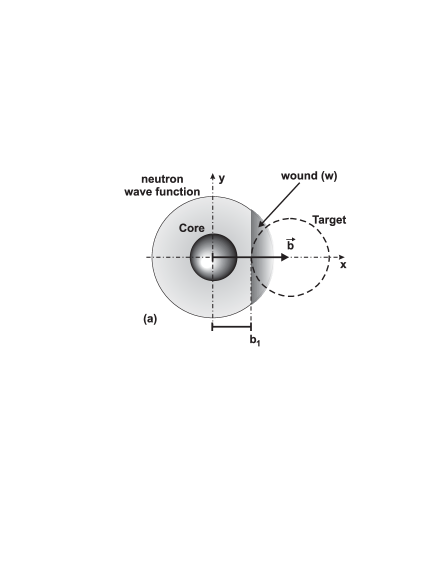
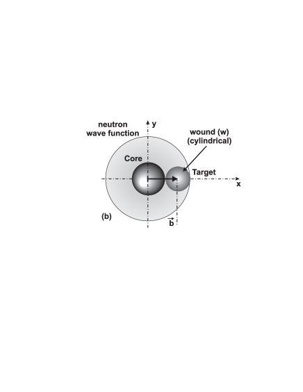
FIG. 1.: Schematic view of the “wound” induced by the projectile-target interaction for (a) a planar cutoff and (b) a cylindrical wound.

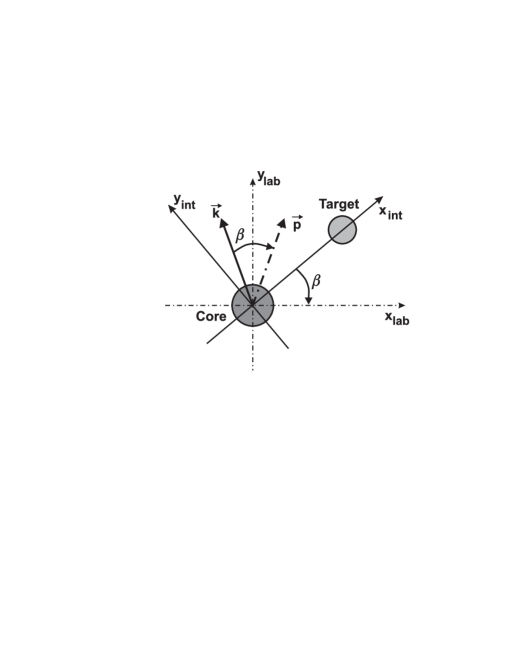
FIG. 2.: Schematic representation of the unitary transformation of Eq. (37) of the momentum vector $\vec{k}$ in the rest frame to the laboratory momentum ($\vec{p}$) by rotation through an angle $\beta$.

FIG. 3.: Single-neutron removal cross sections calculated in the planar cutoff approximation (open circles, dashed line) compared to the experimental values [12, 13] (full circles, solid line) for reactions on a carbon target. The contributions arising from stripping (open triangles, dash-dotted line) and diffraction plus Coulomb dissociation (open diamonds, dotted line) are also detailed.

FIG. 4.: The same as in Fig. 3 but for a cylindrical wound.

FIG. 5.: Core-fragment longitudinal momentum distributions for reactions on a carbon target. The experimental data are taken from ref. [12, 13]. The solid lines correspond to the results of calculations using the sudden approximation model and a planar cutoff.

FIG. 6.: A comparison of the core-fragment longitudinal momentum distributions calculated using the sudden model approximation with a planar cutoff (solid line) and the Glauber model [13] (dash-dotted line). The stripping and diffraction plus Coulomb components (thin solid and dashed lines respectively) in the sudden approximation are also shown.

FIG. 7.: Comparison of the transverse (p_x) momentum distributions calculated within the sudden approximation (solid line) with the Glauber model of ref. [13] (dashed line). The calculated distributions have been convoluted with the experimental effects.

FIG. 8.: Momentum distribution in the projectile rest frame (panels a and c) and in the laboratory frame (panels b and d) for the $s$-wave ground state in ¹⁵C ($S_{n}=1.2$ MeV). Top panels: momentum distributions in the transverse $x$ direction. Bottom panels: momentum distributions in the $y$ direction. Calculations including Coulomb dissociation are shown by the solid lines. Results without Coulomb interaction are represented by dashed lines.

FIG. 9.: Intrinsic momentum distributions (dashed lines) compared with the distributions from the reaction calculation for an $s$-wave valence neutron in ¹⁵C (top panels) and a $d$-wave in ¹⁹N (bottom panels). Projections in the transverse $x$ direction are shown in panels (a) and (c), whilst those in longitudinal direction ($z$) are shown in (b) and (d).

FIG. 10.: Comparison of the transverse (p_x) momentum distributions calculated within the sudden approximation with the data of ref. [13] for ¹⁴B, ^15,16C and ¹⁹N. The decomposition of the total distribution (dashed line) into stripping (dashed-dotted line) and diffraction plus Coulomb (dotted line) components is shown. The calculated distributions, after Monte Carlo filtering to account for the experimental effects, are also displayed (solid line).

FIG. 11.: ¹⁶C core-fragment transverse momentum distributions from reactions of ¹⁷C on a carbon target (data ref. [13]) calculated in the sudden approximation for three spin-parity assignments $J^{\pi}$ for the ground state of ¹⁷C.

FIG. 12.: The same as in Fig.10 but for the perpendicular (p_⟂) momentum distributions calculated within the sudden approximation.

FIG. 13.: Comparison of the measured and predicted longitudinal momentum distributions for single-neutron removal from ¹⁷C on a carbon target. The results obtained using the sudden approximation model are shown by the solid line, whilst those derived using the TCM (see text) are displayed by the dashed line.

FIG. 14.: Evolution of the widths (FWHM) of the longitudinal momentum distributions with the spectrometer angular acceptance. The experimentally observed trend (filled circles, solid line) is compared to the calculations in the sudden approximation model (open circles, dashed lines). Note that the scale for the widths has been expanded.

FIG. 15.: Evolution of the core-fragment longitudinal momentum distribution for reactions of ¹⁶C on carbon as a function of angular acceptances of the spectrometer. The model calculations (solid lines) have been normalized to the maximum number of counts and include, in addition to the finite acceptances, all experimental broadening effects.

FIG. 16.: The same as in Fig. 15 but for ¹⁹N.

REFERENCES

- [1] R. Anne et al., Nucl. Phys. , 125 (1994).
- [2] P.G. Hansen, B.M. Sherrill, Nucl. Phys. , 133 (2001).
- [3] J. S. Al-Khalili, F. Nunes, J. Phys G: Nucl. Part. Phys. 29, 89 (2003).
- [4] R. Serber, Phys. Rev. , 1008 (1947).
- [5] R. J. Glauber, Phys. Rev. , 1515 (1955).
- [6] S.M. Dancoff, Phys. Rev. , 163 (1947).
- [7] G. Faldt, Phys. Rev. , 846 (1970).
- [8] R. Anne et al., Phys. Lett , 55 (1993).
- [9] P.G. Hansen, Phys. Rev. Lett. , 1016 (1996).
- [10] M.S. Hussein, K.W. McVoy, Nucl. Phys. , 124 (1985).
- [11] F. Barranco, E. Vigezzi, Int. School of Heavy Ion Physics. Course: Exotic Nuclei. p. 217, Erice, Italy, 11-20 May 1997. Eds R. A. Broglia, P. G. Hansen, World Scientific.
- [12] E. Sauvan et al., Phys. Lett. B491, 1 (2000).
- [13] E. Sauvan et al., Phys. Rev. C69, 044603 (2004).
- [14] P.G. Hansen, J.A. Tostevin, Ann. Rev. Nucl. Part. Sci. 53, 219 (2003).
- [15] A. Bonaccorso, D.M. Brink, Phys. Rev. C38, 1776(1988).
- [16] A. Bonaccorso, D.M. Brink, Phys. Rev. C44, 1559(1991).
- [17] A. Navin et al., Phys. Rev. Lett. , 5089 (1998).
- [18] J.A. Tostevin, J. Phys. G: Nucl. Part. Phys. , 735 (1999).
- [19] K. Hencken, G. Bertsch, H. Esbensen, Phys. Rev. , 3043 (1996).
- [20] F. Negoita et al., Phys. Rev. , 2082 (1999).
- [21] A. R. Edmonds, , (Princeton Univ. Press) p. 124.
- [22] C.A. Bertulani, G. Baur, Nucl. Phys. , 615 (1988).
- [23] J. Margueron, A. Bonaccorso, D.M. Brink, Nucl. Phys. , 105 (2002).
- [24] B.A. Brown, A. Etchegoyen, W.D.M. Rae, MSU-NSCL Report No. 524 (1988).
- [25] A. De Vismes, P. Roussel-Chomaz, F. Carstoiu, Phys. Rev. C62, 064612 (2000).
- [26] H. Sagawa, N. Takigawa, Phys. Rev. , 985 (1994).
- [27] V. Maddalena et al., Phys Phys. , 024613 (2001).
- [28] U. Datta Pramanik et al., Phys. Lett. B551, 63 (2003).
- [29] A. Bonaccorso, Phys. Rev. C60, 054604(1999).
- [30] J. Enders et al., Phys. Rev. C65, 034318 (2002).
- [31] J. G. Dave, C. R. Gould, Phys. Rev. C28, 2212(1983).
- [32] E. Sauvan, Thèse, Université de Caen, LPC Report LPCC T00-01 (2000).
- [33] N.A. Orr et al., Phys. Rev. Lett. 69, 2050 (1992).
- [34] K. Riisager, in Proc. 3rd Int. Conferences on Radioactive Nuclear Beams, ed. by D.J. Morrisey (Editions Frontières, Gif-sur-Yvette, France, 1993) p. 281.
- [35] J.H. Kelley et al., Phys. Rev. Lett. , 30 (1995).
- [36] J.H. Kelley et al., Nucl. Inst. Meth. , 492 (1997).
- [37] N.A. Orr et al., Phys. Rev. C51, 3116 (1995).
- [38] D.Bazin et al., Phys. Rev. , 2156 (1998).
- [39] J.A. Tostevin et al., Phys. Rev. , 024607 (2002).
- [40] S. Typel, G. Baur, Nucl. Phys. , 486 (1994).