Precision Measurement of the Neutron Spin Asymmetries and Spin-dependent Structure Functions in the Valence Quark Region

Abstract

We report on measurements of the neutron spin asymmetries $A_{1,2}^{n}$ and polarized structure functions $g_{1,2}^{n}$ at three kinematics in the deep inelastic region, with $x=0.33$, $0.47$ and $0.60$ and $Q^{2}=2.7$, $3.5$ and $4.8$ (GeV/c)², respectively. These measurements were performed using a $5.7$ GeV longitudinally-polarized electron beam and a polarized ³He target. The results for $A_{1}^{n}$ and $g_{1}^{n}$ at $x=0.33$ are consistent with previous world data and, at the two higher $x$ points, have improved the precision of the world data by about an order of magnitude. The new $A_{1}^{n}$ data show a zero crossing around $x=0.47$ and the value at $x=0.60$ is significantly positive. These results agree with a next-to-leading order QCD analysis of previous world data. The trend of data at high $x$ agrees with constituent quark model predictions but disagrees with that from leading-order perturbative QCD (pQCD) assuming hadron helicity conservation. Results for $A_{2}^{n}$ and $g_{2}^{n}$ have a precision comparable to the best world data in this kinematic region. Combined with previous world data, the moment $d_{2}^{n}$ was evaluated and the new result has improved the precision of this quantity by about a factor of two. When combined with the world proton data, polarized quark distribution functions were extracted from the new $g_{1}^{n}/F_{1}^{n}$ values based on the quark parton model. While results for $\Delta u/u$ agree well with predictions from various models, results for $\Delta d/d$ disagree with the leading-order pQCD prediction when hadron helicity conservation is imposed.

I INTRODUCTION

Interest in the spin structure of the nucleon became prominent in the 1980’s when experiments at CERN exp:cern-emc and SLAC exp:e080e130 on the integral of the proton polarized structure function $g_{1}^{p}$ showed that the total spin carried by quarks was very small, $\approx(12\pm 17)\%$ exp:cern-emc . This was in contrast to the simple relativistic valence quark model prediction theory:rCQM in which the spin of the valence quarks carries approximately $75\%$ of the proton spin and the remaining $25\%$ comes from their orbital angular momentum. Because the quark model is very successful in describing static properties of hadrons, the fact that the quark spins account for only a small part of the nucleon spin was a big surprise and generated very productive experimental and theoretical activities to the present. Current understanding theory:spin-sr of the nucleon spin is that the total spin is distributed among valence quarks, $q\bar{q}$ sea quarks, their orbital angular momenta, and gluons. This is called the nucleon spin sum rule:

$$S_{z}^{N} = S_{z}^{q}+L_{z}^{q}+J_{z}^{g}=\frac{1}{2}~{},$$ (1)

where $S_{z}^{N}$ is the nucleon spin, $S_{z}^{q}$ and $L_{z}^{q}$ represent respectively the quark spin and orbital angular momentum (OAM), and $J_{z}^{g}$ is the total angular momentum of the gluons. Only about $(20-30)\%$ of the nucleon spin is carried by the spin of the quarks. To further study the nucleon spin, one thus needs to know more precisely how it decomposes into the three components and to measure their dependence on $x$. Here $x$ is the Bjorken scaling variable, which in the quark-parton model theory:partonmodel can be interpreted as the fraction of the nucleon momentum carried by the quark. For a fixed target experiment one has $x={Q^{2}}/({2M\nu})$, with $M$ the nucleon mass, $Q^{2}$ the four momentum transfer squared and $\nu$ the energy transfer from the incident electron to the target. However, due to experimental limitations, precision data have been collected so far only in the low and moderate $x$ regions. In these regions, one is sensitive to contributions from a large amount of $q\bar{q}$ sea and gluons and the nucleon is hard to model. Moreover, at large distances corresponding to the size of a nucleon, the theory of the strong interaction – Quantum Chromodynamics (QCD) – is highly non-perturbative, which makes the investigation of the roles of quark orbital angular momentum (OAM) and gluons in the nucleon spin structure difficult.

Our focus here is the first precise neutron spin structure data in the large $x$ region $x\mathrel{\raise 1.29167pt\hbox{$>$}\mkern-14.0mu\lower 3.01385pt\hbox{$\sim$}}0.4$. For these kinematics, the valence quarks dominate and the ratios of structure functions can be estimated based on our knowledge of the interactions between quarks. More specifically, the virtual photon asymmetry $A_{1}$, defined as

$$A_{1}(x,Q^{2}) \equiv \frac{\sigma_{{1}/{2}}-\sigma_{{3}/{2}}}{\sigma_{{1}/{2}}+\sigma_{{3}/{2}}}$$

(the definitions of $\sigma_{1/2,3/2}$ are given in Appendix A), which at large $Q^{2}$ is approximately the ratio of the polarized and the unpolarized structure functions $g_{1}/F_{1}$, is expected to approach unity as $x\to 1$ in perturbative QCD (pQCD). This is a dramatic prediction, not only because this is the only kinematic region where one can give an absolute prediction for the structure functions based on pQCD, but also because all previous data on the neutron asymmetry $A_{1}^{n}$ in the region $x\mathrel{\raise 1.29167pt\hbox{$>$}\mkern-14.0mu\lower 3.01385pt\hbox{$\sim$}}0.4$ have large uncertainties and are consistent with $A_{1}^{n}\leqslant 0$. Furthermore, because both $q\bar{q}$ sea and gluon contributions are small in this region, it is a relatively clean region to test the valence quark model and to study the role of valence quarks and their OAM contribution to the nucleon spin.

Deep inelastic scattering (DIS) has served as one of the major experimental tools to study the quark and gluon structure of the nucleon. The formalism of unpolarized and polarized DIS is summarized in Appendix A. Within the quark parton model (QPM), the nucleon is viewed as a collection of non-interacting, point-like constituents, one of which carries a fraction $x$ of the nucleon’s longitudinal momentum and absorbs the virtual photon theory:partonmodel . The nucleon cross section is then the incoherent sum of the cross sections for elastic scattering from individual charged point-like partons. Therefore the unpolarized and the polarized structure functions $F_{1}$ and $g_{1}$ can be related to the spin-averaged and spin-dependent quark distributions as book:thomas&weise

$$F_{1}(x,Q^{2})= \frac{1}{2}\sum_{i}e_{i}^{2}q_{i}(x,Q^{2})$$ (2)

and

$$g_{1}(x,Q^{2})= \frac{1}{2}\sum_{i}e_{i}^{2}\Delta q_{i}(x,Q^{2})~{},$$ (3)

where $q_{i}(x,Q^{2})=q_{i}^{\uparrow}(x,Q^{2})+q_{i}^{\downarrow}(x,Q^{2})$ is the unpolarized parton distribution function (PDF) of the $i^{th}$ quark, defined as the probability that the $i^{th}$ quark inside a nucleon carries a fraction $x$ of the nucleon’s momentum, when probed with a resolution determined by $Q^{2}$. The polarized PDF is defined as $\Delta q_{i}(x,Q^{2})=q_{i}^{\uparrow}(x,Q^{2})-q_{i}^{\downarrow}(x,Q^{2})$, where $q_{i}^{\uparrow}(x,Q^{2})$ ($q_{i}^{\downarrow}(x,Q^{2})$) is the probability to find the spin of the $i^{th}$ quark aligned parallel (anti-parallel) to the nucleon spin.

The polarized structure function $g_{2}(x,Q^{2})$ does not have a simple interpretation within the QPM book:thomas&weise . However, it can be separated into leading twist and higher twist terms using the operator expansion method theory:ope :

$$g_{2}(x,Q^{2}) = g_{2}^{WW}(x,Q^{2})+\bar{g}_{2}(x,Q^{2})~{}.$$ (4)

Here $g_{2}^{WW}(x,Q^{2})$ is the leading twist (twist-2) contribution and can be calculated using the twist-2 component of $g_{1}(x,Q^{2})$ and the Wandzura-Wilczek relation theory:g2ww as

$$g_{2}^{WW}(x,Q^{2}) = -g_{1}(x,Q^{2})+\int_{x}^{1}\frac{g_{1}(y,Q^{2})}{y}\mathrm{d}y~{}.$$ (5)

The higher-twist contribution to $g_{2}$ is given by $\bar{g}_{2}$. When neglecting quark mass effects, the higher-twist term represents interactions beyond the QPM, e.g., quark-gluon and quark-quark correlations theory:ope-g2 . The moment of $\bar{g}_{2}$ can be related to the matrix element $d_{2}$ theory:d2def :

$$d_{2} = \int_{0}^{1}\mathrm{d}x~{}x^{2}\Big{[}3g_{2}(x,Q^{2})+2g_{1}(x,Q^{2})\Big{]}$$ (6)

$$= 3\int_{0}^{1}\mathrm{d}x~{}x^{2}\bar{g}_{2}(x,Q^{2})~{}.$$

Hence $d_{2}$ measures the deviations of $g_{2}$ from $g_{2}^{WW}$. The value of $d_{2}$ can be obtained from measurements of $g_{1}$ and $g_{2}$ and can be compared with predictions from Lattice QCD theory:d2lattice , bag models theory:d2bag , QCD sum rules theory:d2QCDSR and chiral soliton models theory:d2chi .

In this paper we first describe available predictions for $A_{1}^{n}$ at large $x$. The experimental apparatus and the data analysis procedure will be described in Section III, IV and V. In Section VI we present results for the asymmetries and polarized structure functions for both ³He and the neutron, a new experimental fit for $g_{1}^{n}/F_{1}^{n}$ and a result for the matrix element $d_{2}^{n}$. Combined with the world proton and deuteron data, polarized quark distribution functions were extracted from our $g_{1}^{n}/F_{1}^{n}$ results. We conclude the paper by summarizing the results for $A_{1}^{n}$ and $\Delta d/d$ and speculating on the importance of the role of quark OAM on the nucleon spin in the kinematic region explored. Some of the results presented here were published previously A1nPRL ; the present publication gives full details on the experiment and all of the neutron spin structure results for completeness.

II Predictions for $A_{1}^{n}$ at large $x$

From Section II.1 to II.6 we present predictions of $A_{1}^{n}$ at large $x$. Data on $A_{1}^{n}$ from previous experiments did not have the precision to distinguish among different predictions, as will be shown in Section II.7.

II.1 SU(6) Symmetric Non-Relativistic Constituent Quark Model

In the simplest non-relativistic constituent quark model (CQM) theory:cqm_org , the nucleon is made of three constituent quarks and the nucleon spin is fully carried by the quark spin. Assuming SU(6) symmetry, the wavefunction of a neutron polarized in the $+z$ direction then has the form theory:su6close :

$$\left|n\uparrow\right\rangle=\frac{1}{\sqrt{2}}\left|d^{\uparrow}(du)_{000}\right\rangle+\frac{1}{\sqrt{18}}\left|d^{\uparrow}(du)_{110}\right\rangle~{}~{}~{}~{}~{}~{}~{}~{}~{}~{}~{}~{}~{}~{}~{}~{}~{}~{}$$ (7)

$$-\frac{1}{3}\left|d^{\downarrow}(du)_{111}\right\rangle-\frac{1}{3}\left|u^{\uparrow}(dd)_{110}\right\rangle+\frac{\sqrt{2}}{3}\left|u^{\downarrow}(dd)_{111}\right\rangle,$$

where the three subscripts are the total isospin, total spin $S$ and the spin projection $S_{z}$ along the $+z$ direction for the ‘diquark’ state. For the case of a proton one needs to exchange the $u$ and $d$ quarks in Eq. (7). In the limit where SU(6) symmetry is exact, both diquark spin states with $S=1$ and $S=0$ contribute equally to the observables of interest, leading to the predictions

$$A_{1}^{p}={5}/{9}~{}~{}\mathrm{and}~{}A_{1}^{n}=0~{};$$ (8)

$$\Delta u/u\to 2/3~{}~{}\mathrm{and}~{}\Delta d/d\to-1/3.$$ (9)

We define $u(x)\equiv u^{p}(x)$, $d(x)\equiv d^{p}(x)$ and $s(x)\equiv s^{p}(x)$ as parton distribution functions (PDF) for the proton. For a neutron one has $u^{n}(x)=d^{p}(x)=d(x)$, $d^{n}(x)=u^{p}(x)=u(x)$ based on isospin symmetry. The strange quark distribution for the neutron is assumed to be the same as that of the proton, $s^{n}(x)=s^{p}(x)=s(x)$. In the following, all PDF’s are for the proton, unless specified by a superscript ‘n’.

In the case of DIS, exact SU(6) symmetry implies the same shape for the valence quark distributions, i.e. $u(x)=2d(x)$. Using Eq. (2) and (30), and assuming that $R(x,Q^{2})$ is the same for the neutron and the proton, one can write the ratio of neutron and proton $F_{2}$ structure functions as

$$R^{np}\equiv\frac{F_{2}^{n}}{F_{2}^{p}}=\frac{u(x)+4d(x)}{4u(x)+d(x)}~{}.$$ (10)

Applying $u(x)=2d(x)$ gives

$$R^{np}={2}/{3}~{}.$$ (11)

However, data on the $R^{np}$ ratio from SLAC data:slacRnp , CERN data:bcdmsRnp ; data:emcRnp ; data:nmcRnp and Fermilab data:e665Rnp disagree with this SU(6) prediction. The data show that $R^{np}(x)$ is a straight line starting with $R^{np}|_{x\to 0}\approx 1$ and dropping to below $1/2$ as $x\to 1$. In addition, $A_{1}^{p}(x)$ is small at low $x$ data:a1pg1p-emc ; data:a1pg1p-smc ; data:a1pa1n-e143 . The fact that $R^{np}|_{x\to 0}\approx 1$ may be explained by the presence of a dominant amount of sea quarks in the low $x$ region and the fact that $A_{1}^{p}|_{x\to 0}\approx 0$ could be because these sea quarks are not highly polarized. At large $x$, however, there are few sea quarks and the deviation from SU(6) prediction indicates a problem with the wavefunction described by Eq. (7). In fact, SU(6) symmetry is known to be broken theory:su6breaking and the details of possible SU(6)-breaking mechanisms is an important open issue in hadronic physics.

II.2 SU(6) Breaking and Hyperfine Perturbed Relativistic CQM

A possible explanation for the SU(6) symmetry breaking is the one-gluon exchange interaction which dominates the quark-quark interaction at short-distances. This interaction was used to explain the behavior of $R^{np}$ near $x\to 1$ and the $\approx 300$-MeV mass shift between the nucleon and the $\Delta(1232)$ theory:su6breaking . Later this was described by an interaction term proportional to $\vec{S}_{i}\cdot\vec{S}_{j}~{}\delta^{3}(\vec{r}_{ij})$, with $\vec{S_{i}}$ the spin of the $i^{th}$ quark, hence is also called the hyperfine interaction, or chromomagnetic interaction among the quarks theory:hyperfine-spin . The effect of this perturbation on the wavefunction is to lower the energy of the $S=0$ diquark state, causing the first term of Eq. (7), $\left|d\uparrow(ud)_{000}\right\rangle^{\mathrm{n}}$, to become more stable and to dominate the high energy tail of the quark momentum distribution that is probed as $x\to 1$. Since the struck quark in this term has its spin parallel to that of the nucleon, the dominance of this term as $x\to 1$ implies $(\Delta d/d)^{\mathrm{n}}\to 1$ and $(\Delta u/u)^{\mathrm{n}}\to-1/3$ for the neutron, while for the proton one has

$$\Delta u/u\to 1~{}\mathrm{and}~{}\Delta d/d\to-1/3\mathrm{~{}~{}as~{}}x\to 1~{}.$$ (12)

One also obtains

$$R^{np}\to{1}/{4}~{}~{}\mathrm{as}~{}x\to 1~{},$$ (13)

which could explain the deviation of $R^{np}(x)$ data from the SU(6) prediction. Based on the same mechanism, one can make the following predictions:

$$A_{1}^{p}\to 1~{}\mathrm{and}~{}A_{1}^{n}\to 1~{}~{}\mathrm{as}~{}x\to 1~{}.$$ (14)

The hyperfine interaction is often used to break SU(6) symmetry in the relativistic CQM (RCQM). In this model, the constituent quarks have non-zero OAM which carries $\approx 25\%$ of the nucleon spin theory:rCQM . The use of RCQM to predict the large $x$ behavior of the nucleon structure functions can be justified by the valence quark dominance, i.e., in the large $x$ region almost all quantum numbers, momentum and the spin of the nucleon are carried by the three valence quarks, which can therefore be identified as constituent quarks. Predictions of $A_{1}^{n}$ and $A_{1}^{p}$ in the large $x$ region using the hyperfine-perturbed RCQM have been achieved theory:cqm .

II.3 Perturbative QCD and Hadron Helicity Conservation

In the early 1970’s, in one of the first applications of perturbative QCD (pQCD), it was noted that as $x\to 1$, the scattering is from a high-energy quark and thus the process can be treated perturbatively theory:farrar . Furthermore, when the quark OAM is assumed to be zero, the conservation of angular momentum requires that a quark carrying nearly all the momentum of the nucleon (i.e. $x\to 1$) must have the same helicity as the nucleon. This mechanism is called hadron helicity conservation (HHC), and is referred to as the leading-order pQCD in this paper. In this picture, quark-gluon interactions cause only the $S=1$, $S_{z}=1$ diquark spin projection component rather than the full $S=1$ diquark system to be suppressed as $x\to 1$, which gives

$$\Delta u/u\to 1~{}\mathrm{and}~{}\Delta d/d\to 1\mathrm{~{}~{}as~{}}x\to 1~{};$$ (15)

$$R^{np}\to\frac{3}{7},~{}A_{1}^{p}\to 1\mathrm{~{}~{}and~{}}A_{1}^{n}\to 1\mathrm{~{}~{}as~{}}x\to 1~{}.$$ (16)

This is one of the few places where pQCD can make an absolute prediction for the $x$-dependence of the structure functions or their ratios. However, how low in $x$ and $Q^{2}$ this picture works is uncertain. HHC has been used as a constraint in a model to fit data on the first moment of the proton $g_{1}^{p}$, giving the BBS parameterization theory:bbs . The $Q^{2}$ evolution was not included in this calculation. Later in the LSS(BBS) parameterization theory:lssbbs , both proton and neutron $A_{1}$ data were fitted directly and the $Q^{2}$ evolution was carefully treated. Predictions for $A_{1}^{n}$ using both BBS and LSS(BBS) parameterizations have been made, as shown in Fig. 1 and 2 in Section II.7.

HHC is based on the assumption that the quark OAM is zero. Recent experimental data on the tensor polarization in elastic $e-^{2}$H scattering data:cebaf-t20 , neutral pion photo-production data:cebaf-gammap and the proton electro-magnetic form factors data:cebaf-F2p ; data:cebaf-Gep disagree with the HHC predictions theory:F2pF1pQCDscaling . It has been suggested that effects beyond leading-order pQCD, such as quark OAM theory:miller ; theory:transpdf ; theory:ji1 ; theory:ji2 , might play an important role in processes involving quark spin flips.

II.4 Predictions from Next-to-Leading Order QCD Fits

In a next-to-leading order (NLO) QCD analysis of the world data theory:lss2001 , parameterizations of the polarized and unpolarized PDFs were performed without the HHC constraint. Predictions of $g_{1}^{p}/F_{1}^{p}$ and $g_{1}^{n}/F_{1}^{n}$ were made using these parameterizations, as shown in Fig. 1 and 2 in Section II.7.

In a statistical approach, the nucleon is viewed as a gas of massless partons (quarks, antiquarks and gluons) in equilibrium at a given temperature in a finite volume, and the parton distributions are parameterized using either Fermi-Dirac or Bose-Einstein distributions. Based on this statistical picture of the nucleon, a global NLO QCD analysis of unpolarized and polarized DIS data was performed theory:stat . In this calculation $\Delta u/u\approx 0.75$, $\Delta d/d\approx-0.5$ and $A_{1}^{p,n}<1$ at $x\to 1$.

II.5 Predictions from Chiral Soliton and Instanton Models

While pQCD works well in high-energy hadronic physics, theories suitable for hadronic phenomena in the non-perturbative regime are much more difficult to construct. Possible approaches in this regime are quark models, chiral effective theories and the lattice QCD method. Predictions for $A_{1}^{n,p}$ have been made using chiral soliton models theory:chi_weigel ; theory:chi_waka and the results of Ref.  theory:chi_waka give $A_{1}^{n}<0$. The prediction that $A_{1}^{p}<0$ has also been made in the instanton model theory:instanton .

II.6 Other Predictions

Based on quark-hadron duality theory:duality-b&g , one can obtain the structure functions and their ratios in the large $x$ region by summing over matrix elements for nucleon resonance transitions. To incorporate SU(6) breaking, different mechanisms consistent with duality were assumed and data on the structure function ratio $R^{np}$ were used to fit the SU(6) mixing parameters. In this picture, $A_{1}^{n,p}\to 1$ as $x\to 1$ is a direct result. Duality predictions for $A_{1}^{n,p}$ using different SU(6) breaking mechanisms were performed in Ref. theory:dual_new . There also exist predictions from bag models theory:bag , as shown in Fig. 1 and 2 in the next section.

II.7 Previous Measurements of $A_{1}^{n}$

A summary of previous $A_{1}^{n}$ measurements is given in

Table 1: Previous measurements of $A_{1}^{n}$.

Experiment	beam	target	$x$	$Q^{2}$
				(GeV/c)2
E142 data:a1ng1n-e142	19.42, 22.66,	3He	0.03-0.6	2
	25.51 GeV; e-
E154 data:a1ng1n-e154	48.3 GeV; e-	3He	0.014-0.7	1-17
HERMES data:a1ng1n-hermes	27.5 GeV; e+	3He	0.023-0.6	1-15
E143 data:a1pa1n-e143	9.7, 16.2,	NH3, ND3	0.024-0.75	0.5-10
	29.1 GeV; e-
E155 data:g1pg1n-e155	48.35 GeV; e-	NH3, LiD3	0.014-0.9	1-40
SMC data:g1n-smc	190 GeV; $\mu^{-}$	C4H10O	0.003-0.7	1-60
		C4D10O

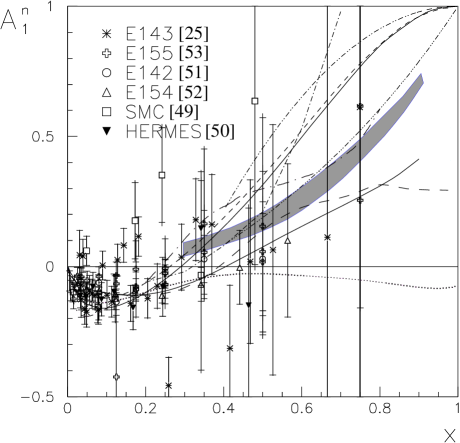
Figure 1: Previous data on $A_{1}^{n}$ data:a1ng1n-e142 ; data:a1ng1n-e154 ; data:g1n-smc ; data:a1ng1n-hermes ; data:a1pa1n-e143 ; data:g1pg1n-e155 and various theoretical predictions: $A_{1}^{n}$ from SU(6) symmetry (solid line at zero) theory:su6close , hyperfine-perturbed RCQM (shaded band) theory:cqm , BBS parameterization at $Q^{2}=4$ (GeV/c)² (higher solid) theory:bbs , LSS(BBS) parameterization at $Q^{2}=4$ (GeV/c)² (dashed) theory:lssbbs , statistical model at $Q^{2}=4$ (GeV/c)² (long-dashed) theory:stat , quark-hadron duality using two different SU(6) breaking mechanisms (dash-dot-dotted and dash-dot-dot-dotted)theory:dual_new , and non-meson cloudy bag model (dash-dotted) theory:bag ; $g_{1}^{n}/F_{1}^{n}$ from LSS2001 parameterization at $Q^{2}=5$ (GeV/c)² (lower solid) theory:lss2001 and from chiral soliton models theory:chi_weigel at $Q^{2}=3$ (GeV/c)² (long dash-dotted) and theory:chi_waka at $Q^{2}=4.8$ (GeV/c)² (dotted).

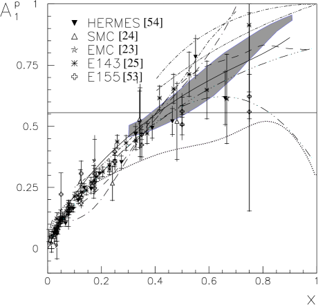
Figure 2: World data on $A_{1}^{p}$ data:a1pa1n-e143 ; data:a1pg1p-emc ; data:a1pg1p-smc ; data:g1pg1n-e155 ; data:g1p-hermes and predictions for $g_{1}^{p}/F_{1}^{p}$ at $Q^{2}=5$ (GeV/c)² from the E155 experimental fit (long dash-dot-dotted) data:g1pg1n-e155 and a new fit as described in Section VI.2 (long dash-dot-dot-dotted). The solid curve corresponds to the prediction for $g_{1}^{n}/F_{1}^{n}$ from LSS(2001) parameterization at $Q^{2}=5$ (GeV/c)². Other curves are the same as in Fig. 1 except that there is no prediction for the proton from BBS and LSS(BBS) parameterizations.

Table 1. The data on $A_{1}^{n}$ and $A_{1}^{p}$ are plotted in Fig. 1 and 2 along with theoretical calculations described in previous sections. Since the $Q^{2}$-dependence of $A_{1}$ is small and $g_{1}/F_{1}\approx A_{1}$ in DIS, data for $g_{1}^{n}/F_{1}^{n}$ and $g_{1}^{p}/F_{1}^{p}$ are also shown and all data are plotted without evolving in $Q^{2}$. As becomes obvious in Fig. 1, the precision of previous $A_{1}^{n}$ data at $x>0.4$ from SMC data:g1n-smc , HERMES data:a1ng1n-hermes and SLAC data:a1ng1n-e142 ; data:a1pa1n-e143 ; data:a1ng1n-e154 is not sufficient to distinguish among different predictions.

III THE EXPERIMENT

We report on an experiment exp:e99117 carried out at in the Hall A of Thomas Jefferson National Accelerator Facility (Jefferson Lab, or JLab). The goal of this experiment was to provide precise data on $A_{1}^{n}$ in the large $x$ region. We have measured the inclusive deep inelastic scattering of longitudinally polarized electrons off a polarized ³He target, with the latter being used as an effective polarized neutron target. The scattered electrons were detected by the two standard High Resolution Spectrometers (HRS). The two HRS were configured at the same scattering angles and momentum settings to double the statistics. Data were collected at three $x$ points as shown in Table 2. Both longitudinal and transverse electron asymmetries were measured, from which $A_{1}$, $A_{2}$, $g_{1}/F_{1}$ and $g_{2}/F_{1}$ were extracted using Eq. (48–51).

Table 2: Kinematics of the experiment. The beam energy was $E=5.734$ GeV. $E^{\prime}$ and $\theta$ are the nominal momentum and angle of the scattered electrons. $\langle x\rangle$, $\langle Q^{2}\rangle$ and $\langle W^{2}\rangle$ are values averaged over the spectrometer acceptance.

$\langle x\rangle$	0.327	0.466	0.601
$E^{\prime}$	1.32	1.72	1.455
$\theta$	$35^{\circ}$	$35^{\circ}$	$45^{\circ}$
$\langle Q^{2}\rangle$ (GeV/c)2	2.709	3.516	4.833
$\langle W^{2}\rangle$ (GeV)2	6.462	4.908	4.090

III.1 Polarized ³He as an Effective Polarized Neutron

As shown in Fig. 1, previous data on $A_{1}^{n}$ did not have sufficient precision in the large $x$ region. This is mainly due to two experimental limitations. Firstly, high polarization and luminosity required for precision measurements in the large $x$ region were not available previously. Secondly, there exists no free dense neutron target suitable for a scattering experiment, mainly because of the neutron’s short lifetime ($\approx 886$ sec). Therefore polarized nuclear targets such as ${}^{2}\vec{\mathrm{H}}$ or ${}^{3}\vec{\mathrm{He}}$ are commonly used as effective polarized neutron targets. Consequently, nuclear corrections need to be applied to extract neutron results from nuclear data.

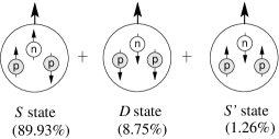
Figure 3: An illustration of ³He wavefunction. The $S$, $S^{\prime}$ and $D$ state contributions are from calculations using the AV18 two-nucleon interaction and the Tucson-Melbourne three-nucleon force, as given in Ref. theory:PnPp_nogga .

For a polarized deuteron, approximately half of the deuteron spin comes from the proton and the other half comes from the neutron. Therefore the neutron results extracted from the deuteron data have a significant uncertainty coming from the error in the proton data. The advantage of using ${}^{3}\vec{\mathrm{He}}$ is that the two protons’ spins cancel in the dominant $S$ state of the ³He wavefunction, thus the spin of the ³He comes mainly ($>87\%$) from the neutron theory:PnPp_friar ; theory:PnPp_nogga , as illustrated in Fig. 3. As a result, there is less model dependence in the procedure of extracting the spin-dependent observables of the neutron from ³He data. At large $x$, the advantage of using a polarized ³He target is more prominent in the case of $A_{1}^{n}$. In this region almost all calculations show that $A_{1}^{n}$ is much smaller than $A_{1}^{p}$, therefore the $A_{1}^{n}$ results extracted from nuclear data are more sensitive to the uncertainty in the proton data and the nuclear model being used.

In the large $x$ region, the cross sections are small because the parton densities drop dramatically as $x$ increases. In addition, the Mott cross section, given by Eq. 29, is small at large $Q^{2}$. To achieve a good statistical precision, high luminosity is required. Among all laboratories which are equipped with a polarized ³He target and are able to perform a measurement of the neutron spin structure, the polarized electron beam at JLab, combined with the polarized ³He target in Hall A, provides the highest polarized luminosity in the world thesis:zheng . Hence it is the best place to study the large $x$ behavior of the neutron spin structure.

III.2 The Accelerator and the Polarized Electron Source

JLab operates a continuous-wave electron accelerator that recirculates the beam up to five times through two super-conducting linear accelerators. Polarized electrons are extracted from a strained GaAs photocathode exp:polestrain illuminated by circularly polarized light, providing a polarized beam of $(70-80)\%$ polarization and $\approx 200\mu A$ maximum current to experimental halls A, B and C. The maximum beam energy available at JLab so far is 5.7 GeV, which was also the beam energy used during this experiment.

III.3 Hall A Overview

The basic layout of Hall A during this experiment is shown in Fig. 4. The major instrumentation exp:NIM includes beamline equipment, the target and two HRSs.

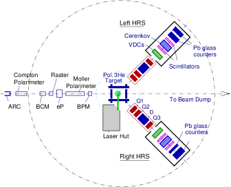
Figure 4: (Color online) Top-view of the experimental hall A (not to scale).

The beamline starts after the arc section of the accelerator where the beam is bent into the hall, and ends at the beam dump. The arc section can be used for beam energy measurement, as will be described in Section III.4. After the arc section, the beamline is equipped with a Compton polarimeter, two Beam Current Monitors (BCM) and an Unser monitor for absolute beam current measurement, a fast raster, the eP device for beam energy measurement, a M$\o$ller polarimeter and two Beam Position Monitors (BPM). These beamline elements, together with spectrometers and the target, will be described in detail in the following sections.

III.4 Beam Energy Measurement

The energy of the beam was measured absolutely by two independent methods - ARC and eP exp:NIM ; exp:NIM-52 . Both methods can provide a precision of $\delta E_{beam}/E_{beam}\approx 2\times 10^{-4}$. For the ARC method exp:NIM ; thesis:marchand , the deflection of the beam in the arc section of the beamline is used to determine the beam energy. In the eP measurement exp:NIM ; thesis:ravel the beam energy is determined by the measurement of the scattered electron angle $\theta_{e}$ and the recoil proton angle $\theta_{p}$ in ¹H$(e,e^{\prime}p)$ elastic scattering.

III.5 Beam Polarization Measurement

Two methods were used during this experiment to measure the electron beam polarization. The M$\o$ller polarimeter exp:NIM measures M$\o$ller scattering of the polarized electron beam off polarized atomic electrons in a magnetized foil. The cross section of this process depends on the beam and target polarizations. The polarized electron target used by the M$\o$ller polarimeter was a ferromagnetic foil, with its polarization determined from foil magnetization measurements. The M$\o$ller measurement is invasive and typically takes an hour, providing a statistical accuracy of about $0.2\%$. The systematic error comes mainly from the error in the foil target polarization. An additional systematic error is due to the fact that the beam current used during a M$\o$ller measurement ($\approx 0.5\mu$A) is lower than that used during the experiment. The total relative systematic error was $\approx 3.0\%$ during this experiment.

During a Compton polarimeter exp:NIM ; thesis:baylac measurement, the electron beam is scattered off a circularly polarized photon beam and the counting rate asymmetry of the Compton scattered electrons or photons between opposite beam helicities is measured. The Compton polarimeter measures the beam polarization concurrently with the experiment running in the hall.

The Compton polarimeter consists of a magnetic chicane which deflects the electron beam away from the scattered photons, a photon source, an electromagnetic calorimeter and an electron detector. The photon source was a 200 mW laser amplified by a resonant Fabry-Perot cavity. During this experiment the maximum gain of the cavity reached $G_{max}=7500$, leading to a laser power of $1500$ W inside the cavity. The circular polarization of the laser beam was $>99\%$ for both right and left photon helicity states. The asymmetry measured in Compton scattering at JLab with a $1.165$ eV photon beam and the $5.7$ GeV electron beam used by this experiment had a mean value of $\approx 2.2\%$ and a maximum of $9.7\%$. For a 12 $\mu$A beam current, one hour was needed to reach a relative statistical accuracy of $(\Delta P_{b})_{stat}/P_{b}\approx 1\%$. The total systematic error was $(\Delta P_{b})_{sys}/P_{b}\approx 1.6\%$ during this experiment.

The average beam polarization during this experiment was extracted from a combined analysis of 7 M$\o$ller and 53 Compton measurements. A value of $(79.7\pm 2.4)\%$ was used in the final DIS analysis.

III.6 Beam Helicity

The helicity state of electrons is regulated every $33$ ms at the electron source. The time sequence of the electrons’ helicity state is carried by helicity signals, which are sent to experimental halls and the data acquisition (DAQ) system. Since the status of the helicity signal (H+ or H- pulses) has either the same or the opposite sign as the real electron helicity, the absolute helicity state of the beam needs to be determined by other methods, as will be described later.

There are two modes – toggle and pseudorandom – which can be used for the pulse sequence of the helicity signal. In the toggle mode, the helicity alternates every $33$ ms. In the pseudorandom mode, the helicity alternates randomly at the beginning of each pulse pair, of which the two pulses must have opposite helicities in order to equalize the numbers of the H+ and H- pulses. The purpose of the pseudorandom mode is to minimize any possible time-dependent systematic errors.

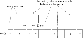
Figure 5: Helicity signal and the helicity status of DAQ in toggle (top) and pseudorandom (bottom) modes.

Fig. 5 shows the helicity signals and the helicity states of the DAQ system for the two regulation modes.

There is a half-wave plate at the polarized source which can be inserted to reverse the helicity of the laser illuminating the photocathode hence reverse the helicity of electron beam. During the experiment this half-wave plate was inserted for half of the statistics to minimize possible systematic effects related to the beam helicity.

The scheme described above was used to monitor the relative changes of the helicity state. The absolute sign of the electrons’ helicity states during each of the H+ and H- pulses were confirmed by measuring a well known asymmetry and comparing the measured asymmetry with its prediction, as will be presented in Section V.2 and V.3.

III.7 Beam Charge Measurement and Charge Asymmetry Feedback

The beam current was measured by the BCM system located upstream of the target on the beamline. The BCM signals were fed to scaler inputs and were inserted in the data stream.

Possible beam charge asymmetry measured at Hall A can be caused by the timing asymmetry of the DAQ system, or by the timing and the beam intensity asymmetries at the polarized electron source. The beam intensity asymmetry originates from the intensity difference between different helicity states of the circularly polarized laser used to strike the photocathode. Although the charge asymmetry can be corrected for to first order, there may exist unknown non-linear effects which can cause a systematic error in the measured asymmetry. Thus the beam charge asymmetry should be minimized. This was done by using a separate DAQ system initially developed for the parity-violation experiments exp:parityQasym , called the parity DAQ. The parity DAQ used the measured charge asymmetry in Hall A to control the orientation of a rotatable half-wave plate located before the photocathode at the source, such that intensities for each helicity state of the polarized laser used to strike the photocathode were adjusted accordingly. The parity DAQ was synchronized with the two HRS DAQ systems so that the charge asymmetry in the two different helicity states could be monitored for each run. The charge asymmetry was typically controlled to be below $2\times 10^{-4}$ during this experiment.

III.8 Raster and Beam Position Monitor

To protect the target cell from being damaged by the effect of beam-induced heating, the beam was rastered at the target. The raster consists a pair of horizontal and vertical air-core dipoles located upstream of the target on the beamline, which can produce either a rectangular or an elliptical pattern. We used a raster pattern distributed uniformly over a circular area with a radius of 2 mm.

The position and the direction of the beam at the target were measured by two BPMs located upstream of the target exp:NIM . The beam position can be measured with a precision of 200 $\mu$m with respect to the Hall A coordinate system. The beam position and angle at the target were recorded for each event.

III.9 High Resolution Spectrometers

The Hall A High Resolution Spectrometer (HRS) systems were designed for detailed investigations of the structure of nuclei and nucleons. They provide high resolution in momentum and in angle reconstruction of the reaction product as well as being able to be operated at high luminosity. For each spectrometer, the vertically bending design includes two quadrupoles followed by a dipole magnet and a third quadrupole. All quadrupoles and the dipole are superconducting. Both HRSs can provide a momentum resolution better than $2\times 10^{-4}$ and a horizontal angular resolution better than 2 mrad with a design maximum central momentum of 4 GeV/c exp:NIM . By convention, the two spectrometers are identified as the left and the right spectrometers based on their position when viewed looking downstream.

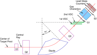
Figure 6: (Color online) Schematic layout of the left HRS and detector package (not to scale).

The basic layout of the left HRS is shown in Fig. 6. The detector package is located in a large steel and concrete detector hut following the last magnet. For this experiment the detector package included (1) two scintillator planes S1 and S2 to provide a trigger to activate the DAQ electronics; (2) a set of two Vertical Drift Chambers (VDC) exp:vdc for particle tracking; (3) a gas $\breve{\mathrm{C}}$erenkov detector to provide particle identification (PID) information; and (4) a set of lead glass counters for additional PID. The layout of the right HRS is almost identical except a slight difference in the geometry of the gas $\breve{\mathrm{C}}$erenkov detector and the lead glass counters.

III.10 Particle Identification

For this experiment the largest background came from photo-produced pions. We refer to PID in this paper as the identification of electrons from pions. PID for each HRS was accomplished by a CO₂ threshold gas $\breve{\mathrm{C}}$erenkov detector and a double-layered lead glass shower detector.

The two $\breve{\mathrm{C}}$erenkov detectors, one on each HRS, were operated with CO₂ at atmospheric pressure. The refraction index of the CO₂ gas was 1.00041, giving a threshold momentum of $\approx 17$ MeV/c for electrons and $\approx 4.8$ GeV/c for pions. The incident particles on each HRS were also identified by their energy deposits in the lead glass shower detector.

Since $\breve{\mathrm{C}}$erenkov detectors and lead glass shower detectors are based on different mechanisms and their PID efficiencies are not correlated book:partdet , we extracted the PID efficiency of the lead glass counters by using electron events selected by the $\breve{\mathrm{C}}$erenkov detector, and vice versa. Fig. 7 shows a spectrum of the summed ADC signal of the left HRS gas $\breve{\mathrm{C}}$erenkov detector, without a cut on the lead glass signal and after applying such lead glass electron and pion cuts. The spectrum from the right HRS is similar.

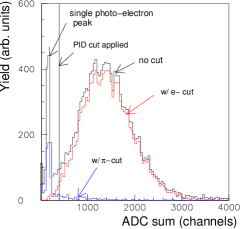
Figure 7: (Color online) Summed ADC signal of the left HRS gas $\breve{\mathrm{C}}$erenkov detector: without cuts, after lead glass counters electron cut and after pion cut. The vertical line shows a cut $\sum{\mathrm{ADC}_{i}}>400$ applied to select electrons.

Fig. 8 shows the distribution of the energy deposit in the two layers of the right HRS lead glass counters, without a $\breve{\mathrm{C}}$erenkov cut, and after $\breve{\mathrm{C}}$erenkov electron and pion cuts.

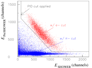
Figure 8: (Color online) Energy deposited in the first layer (preshower) vs that in the second layer (shower) of lead glass counters in the right HRS. The two blobs correspond to the spectrum with a tight gas $\breve{\mathrm{C}}$erenkov ADC electron cut and with a pion cut applied. The lines show the boundary of the two-dimensional cut used to select electrons in the data analysis.

Detailed PID analysis was done both before and during the experiment. The PID performance of each detector is characterized by the electron detection efficiency $\eta_{e}$ and the pion rejection factor $\eta_{\pi,\mathrm{rej}}$, defined as the number of pions needed to cause one pion contamination event. In the HRS central momentum range of $0.8<p_{0}<2.0$ (GeV/c), the PID efficiencies for the left HRS were found to be
$\diamond$ Gas $\breve{\mathrm{C}}$erenkov:   $\eta_{\pi,\mathrm{rej}}>770$ at $\eta_{e}=99.9\%$;
$\diamond$ Lead glass counters: $\eta_{\pi,\mathrm{rej}}\approx 38$ at $\eta_{e}=98\%$;
$\diamond$ Combined: $\eta_{\pi,\mathrm{rej}}>3\times 10^{4}$ at $\eta_{e}=98\%$.

and for the right HRS were
$\diamond$ Gas $\breve{\mathrm{C}}$erenkov:   $\eta_{\pi,\mathrm{rej}}=900$ at $\eta_{e}=99\%$;
$\diamond$ Lead glass counters: $\eta_{\pi,\mathrm{rej}}\approx 182$ at $\eta_{e}=98\%$;
$\diamond$ Combined: $\eta_{\pi,\mathrm{rej}}>1.6\times 10^{5}$ at $\eta_{e}=97\%$.

III.11 Data Acquisition System

We used the CEBAF Online Data Acquisition (CODA) system exp:coda for this experiment. In the raw data file, data from the detectors, the beamline equipment, and from the slow control software were recorded. The total volume of data accumulated during the two-month running period was about 0.6 TBytes. Data from the detectors were processed using an analysis package called Experiment Scanning Program for hall A Collaboration Experiments (ESPACE) exp:espace . ESPACE was used to filter raw data, to make histograms for reconstructed variables, to export variables into ntuples for further analysis, and to calibrate experiment-specific detector constants. It also provided the possibility to apply conditions on the incoming data. The information from scaler events was used to extract beam charge and DAQ deadtime corrections.

IV The Polarized $\bm{{}^{3}\mathrm{He}}$ Target

Polarized ³He targets are widely used at SLAC, DESY, MAINZ, MIT-Bates and JLab to study the electromagnetic structure and the spin structure of the neutron. There exist two major methods to polarize ³He nuclei. The first one uses the metastable-exchange optical pumping technique targ:metaexch . The second method is based on optical pumping targ:optpump and spin exchange targ:spinexch . It has been used at JLab since 1998 exp:e94010 , and was used here.

The ${}^{3}\vec{\mathrm{He}}$ target at JLab Hall A uses the same design as the SLAC ${}^{3}\vec{\mathrm{He}}$ target thesis:romalis . The first step to polarize ³He nuclei is to polarize an alkali metal vapor (rubidium was used at JLab as well as at SLAC) by optical pumping targ:optpump with circularly polarized laser light. Depending on the photon helicity, the electrons in the Rb atoms will accumulate at either the $F=3,m_{F}=3$ or the $F=3,m_{F}=-3$ level (here $F$ is the atom’s total spin and $m_{F}$ is its projection along the magnetic field axis). The polarization is then transfered to the ³He nuclei through the spin exchange mechanism targ:spinexch during collisions between Rb atoms and the ³He nuclei. Under operating conditions the ³He density is about $10^{20}$ nuclei/cm³ and the Rb density is about $10^{14}$ atoms/cm³.

To minimize depolarization effects caused by the unpolarized light emitted from decay of the excited electrons, N₂ buffer gas was added to provide a channel for the excited electrons to decay to the ground state without emitting photons targ:optpump . In the presence of N₂, electrons decay through collisions between the Rb atoms and N₂ molecules, which is usually referred to as non-radiative quenching. The number density of N₂ was about $1\%$ of that of ³He.

IV.1 Target Cells

The target cells used for this experiment were 25-cm long pressurized glass cells with $\sim 130$-$\mu$m thick end windows.

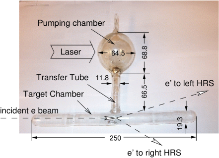
Figure 9: (Color online) JLab target cell, geometries are given in mm for cell #2 used in this experiment.

Table 3: Target cell characteristics. Symbols are: $V_{p}$ pumping chamber volume in cm³; $V_{t}$ target chamber volume in cm³; $V_{tr}$ transfer tube volume in cm³; $V_{0}$ total volume in cm³; $L_{tr}$ transfer tube length in cm; $n_{0}$: ³He density in amg at room temperature (1 amg $=2.69\times 10^{-19}/$cm³ which corresponds to the gas density at the standard pressure and $T=0^{\circ}$C); lifetime is in hours.

Name	$V_{p}$	$V_{t}$	$V_{tr}$	$V_{0}$	$L_{tr}$	$n_{0}$	lifetime
Cell #1	116.7	51.1	3.8	171.6	6.574	9.10	49
Cell #2	116.1	53.5	3.9	173.5	6.46	8.28	44
uncertainty	1.5	1.0	0.25	1.8	0.020	2%	1

The cell consisted of two chambers, a spherical upper chamber which holds the Rb vapor and in which the optical pumping occurs, and a long cylindrical chamber where the electron beam passes through and interacts with the polarized ³He nuclei. Two cells were used for this experiment. Figure 9 is a picture of the first cell with dimensions shown in mm. Table 3 gives the cell volumes and densities.

IV.2 Target Setup

Figure 10 is a schematic diagram of the target setup. There were two pairs of Helmholtz coils to provide a 25 G main holding field, with one pair oriented perpendicular and the other parallel to the beamline (only the perpendicular pair is shown). The holding field could be aligned in any horizontal direction with respect to the incident electron beam. The coils were excited by two power supplies in the constant voltage mode. The coil currents were continuously measured and recorded by the slow control system.

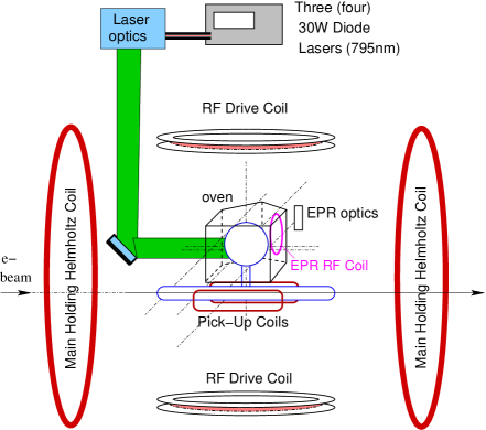
Figure 10: (Color online) Target setup overview (schematic).

The cell was held at the center of the Helmholtz coils with its pumping chamber mounted inside an oven heated to $170^{\circ}$C in order to vaporize the Rb. The lasers used to polarize the Rb were three 30 W diode lasers tuned to a wavelength of 795 nm. The target polarization was measured by two independent methods – the NMR (Nuclear Magnetic Resonance) exp:NIM ; exp:e94010 ; thesis:kramer and the EPR (Electro Paramagnetic Resonance) exp:NIM ; exp:e94010 ; PRA03004 ; thesis:zheng polarimetry. The NMR system consisted of one pair of pick-up coils (one on each side of the cell target chamber), one pair of RF coils and the associated electronics. The RF coils were placed at the top and the bottom of the scattering chamber, oriented in the horizontal plane, as shown in Fig. 10. The EPR system shared the RF coils with the NMR system. It consisted of one additional RF coil to induce light signal emission from the pumping chamber, a photodiode and the related optics to collect the light, and associated electronics for signal processing.

IV.3 Laser System

The laser system used during this experiment consisted of seven diode lasers – three for longitudinal pumping, three for transverse pumping and one spare. To protect the diode lasers from radiation damage from the electron beam, as well as to minimize the safety issues related to the laser hazard, the diode lasers and the associated optics system were located in a concrete laser hut located on the right side of the beamline at $90^{\circ}$, as shown in Fig. 4. The laser optics had seven individual lines, each associated with one diode laser. All seven optical lines were identical and were placed one on top of the other on an optics table inside the laser hut. Each optical line consisted of one focusing lens to correct the angular divergence of the laser beam, one beam-splitter to linearly polarize the lasers, two mirrors to direct them, three quarter waveplates to convert linear polarization to circular polarization, and two half waveplates to reverse the laser helicity. Figure 11 shows a schematic diagram

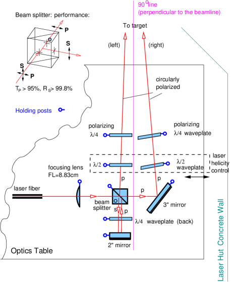
Figure 11: (Color online) Laser polarizing optics setup (schematic) for the Hall A polarized ³He target.

of one optics line.

Under the operating conditions for either longitudinal or transverse pumping, the original beam of each diode laser was divided into two by the beam-splitter. Therefore there were a total of six polarized laser beams entering the target. The diameter of each beam was about 5 cm which approximately matched the size of the pumping chamber. The target was about 5 m away from the optical table. For the pumping of the transversely polarized target, all these laser beams went directly towards the pumping chamber of the cell through a window on the side of the target scattering chamber enclosure. For longitudinal pumping, they were guided towards the top of the scattering chamber, then were reflected twice and finally reached the cell pumping chamber.

IV.4 NMR Polarimetry

The polarization of the ³He was determined by measuring the ³He Nuclear Magnetic Resonance (NMR) signal. The principle of NMR polarimetry is the spin reversal of ³He nuclei using the Adiabatic Fast Passage (AFP) targ:AFP technique. At resonance this spin reversal will induce an electromagnetic field and a signal in the pick-up coil pair. The signal magnitude is proportional to the polarization of the ³He and can be calibrated by performing the same measurement on a water sample, which measures the known thermal polarization of protons in water. The systematic error of the NMR measurement was about $3\%$, dominated by the error in the water calibration thesis:kramer .

IV.5 EPR Polarimetry

In the presence of a magnetic field, the Zeeman splitting of Rb, characterized by the Electron-Paramagnetic Resonance frequency $\nu_{\mathrm{EPR}}$, is proportional to the field magnitude. When ³He nuclei are polarized ($P\approx 40\%$), their spins generate a small magnetic field $B_{{}^{3}\mathrm{He}}$ of the order of $\approx 0.1$ Gauss, super-imposed on the main holding field $B_{H}=25$ Gauss. During an EPR measurement PRA03004 the spin of the ³He is flipped by AFP, hence the direction of $B_{{}^{3}\mathrm{He}}$ is reversed and the change in the total field magnitude causes a shift in $\nu_{\mathrm{EPR}}$. This frequency shift $\delta\nu_{\mathrm{EPR}}$ is proportional to the ³He polarization in the pumping chamber. The ³He polarization in the target chamber is calculated using a model which describes the polarization diffusion from the pumping chamber to target chamber. The value of the EPR resonance frequency $\nu_{\mathrm{EPR}}$ can also be used to calculate the magnetic field magnitude. The systematic error of the EPR measurement was about $3\%$, which came mainly from uncertainties in the cell density and temperature, and from the diffusion model.

IV.6 Target Performance

The target polarizations measured during this experiment are shown in Fig. 12. Results from the two polarimetries are in

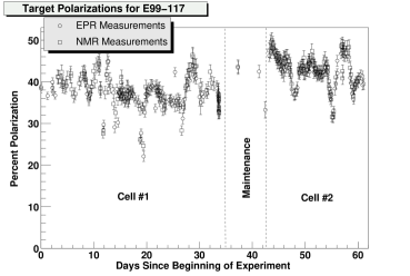
Figure 12: Target polarization, starting June 1 of 2001, as measured by EPR and NMR polarimetries.

good agreement and the average target polarization in beam was $(40.0\pm 2.4)\%$. In a few cases the polarization measurement itself caused an abrupt loss in the polarization. This phenomenon may be the so-called “masing effect” thesis:romalis due to non-linear couplings between the ³He spin rotation and conducting components inside the scattering chamber, e.g., the NMR pick-up coils, and the “Rb-ring” formed by the rubidium condensed inside the cell at the joint of the two chambers. This masing effect was later suppressed by adding coils to produce an additional field gradient.

V Data Analysis

In this section we present the analysis procedure leading to the final results in Section VI. We start with the analysis of elastic scattering, the $\Delta(1232)$ transverse asymmetry, and the check for false asymmetry. Next, the DIS analysis and radiative corrections are presented. Finally we describe nuclear corrections which were used to extract neutron structure functions from the ³He data.

V.1 Analysis Procedure

The procedure to extract the electron asymmetries from our data is outlined in Fig. 13.

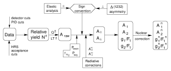
Figure 13: Procedure for asymmetry analysis.

From the raw data one first obtains the helicity-dependent electron yield $N^{\pm}$ using acceptance and PID cuts. The efficiencies associated with these cuts are not helicity-dependent, hence are not corrected for in the asymmetry analysis. The yield is then corrected for the helicity-dependent integrated beam charge $Q^{\pm}$ and the livetime of the DAQ system $\mathrm{LT}^{\pm}$. The asymmetry of the corrected yield is the raw asymmetry $A_{raw}$. Next, to go from $A_{raw}$ to the physics asymmetries $A_{\parallel}$ and $A_{\perp}$, four factors need to be taken into account: the beam polarization $P_{b}$, the target polarization $P_{t}$, the nitrogen dilution factor $f_{\mathrm{N}_{2}}$ due to the unpolarized nitrogen nuclei mixed with the polarized ³He gas, and a sign based on the knowledge of the absolute state of the electron helicity and the target spin direction:

$$A_{\parallel,\perp} = \pm\frac{A_{raw}}{f_{\mathrm{N}_{2}}P_{b}P_{t}}$$ (17)

The results of the beam and the target polarization measurements have been presented in previous sections. The nitrogen dilution factor is obtained from data taken with a reference cell filled with nitrogen. The sign of the asymmetry is described by “the sign convention”. The sign convention for parallel asymmetries was obtained from the elastic scattering asymmetry and that for perpendicular asymmetries was from the $\Delta(1232)$ asymmetry analysis, as will be described in Sections V.2 and V.3. The physics asymmetries $A_{\parallel}$ and $A_{\perp}$, after corrections for radiative effects, were used to calculate $A_{1}$ and $A_{2}$ and the structure function ratios $g_{1}/F_{1}$ and $g_{2}/F_{1}$ using Eq. (48—51). Then the last step is to apply nuclear corrections in order to extract the neutron asymmetries and the structure function ratios from the ³He results, as will be described in Section V.6.

Although the main goal of this experiment was to provide precise data on the asymmetries, cross sections were also extracted from the data. The procedure for the cross section analysis is outlined in Fig. 14. One first determines the absolute yield of $\vec{e}-\vec{{}^{3}\mathrm{He}}$ inclusive scattering from the raw data. Unlike the asymmetry analysis, corrections need to be made for the detector and PID efficiencies and the spectrometer acceptance. A Monte-Carlo simulation is used to calculate the spectrometer

Figure 14: Procedure for cross section analysis.

acceptance based on a transport model for the HRS exp:NIM with radiative effects taken into account. One then subtracts the yield of $e-\mathrm{N}$ scattering caused by the N₂ nuclei in the target. The clean $\vec{e}-\vec{{}^{3}\mathrm{He}}$ yield is then corrected for the helicity-averaged beam charge and the DAQ livetime to give cross section results. Using world fits for the unpolarized structure functions (form factors) of ³He, one can calculate the expected DIS (elastic) cross section from the Monte-Carlo simulation and compare to the data.

V.2 Elastic Analysis

Data for $\vec{e}-^{3}\vec{\mathrm{He}}$ elastic scattering were taken on a longitudinally polarized target with a beam energy of 1.2 GeV. The scattered electrons were detected at an angle of $20^{\circ}$. The formalism for the cross sections and asymmetries are summarized in Appendix B. Results for the elastic asymmetry were used to check the product of beam and target polarizations, as well as to determine the sign convention for different beam-helicity states and target spin directions.

The raw asymmetry was extracted from the data by

$$A_{raw} = \frac{\frac{N^{+}}{Q^{+}LT^{+}}-\frac{N^{-}}{Q^{-}LT^{-}}}{\frac{N^{+}}{Q^{+}LT^{+}}+\frac{N^{-}}{Q^{-}LT^{-}}}$$ (18)

with $N^{\pm}$, $Q^{\pm}$ and $LT^{\pm}$ the helicity-dependent yield, beam charge and livetime correction, respectively. The elastic asymmetry is

$$A_{\parallel}^{el} = \pm\frac{A_{raw}}{f_{\mathrm{N}_{2}}f_{QE}P_{b}P_{t}}$$ (19)

with $f_{\mathrm{N}_{2}}=0.975\pm 0.003$ the N₂ dilution factor determined from data taken with a reference cell filled with nitrogen, and $P_{b}$ and $P_{t}$ the beam and target polarization, respectively. A cut in the invariant mass $|{W-M_{{}^{3}\mathrm{He}}}|<6$ (MeV) was used to select elastic events. Within this cut there are a small amount of quasi-elastic events and $f_{QE}>0.99$ is the quasi-elastic dilution factor used to correct for this effect.

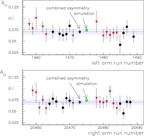
Figure 15: (Color online) Elastic parallel asymmetry results for the two HRS. The kinematics are $E=1.2$ GeV and $\theta=20^{\circ}$. A cut in the invariant mass $|{W-M_{{}^{3}\mathrm{He}}}|<6$ (MeV) was used to select elastic events. Data from runs with beam half-wave plate inserted are shown as triangles. The error bars shown are total errors including a $4.5\%$ systematic uncertainty, which is dominated by the error of the beam and target polarizations. The combined asymmetry and its total error from $\approx 20$ runs are shown by the horizontal solid and dashed lines, respectively, as well as the solid circle as labeled thesis:zheng .

The sign on the right hand side of Eq. (19) depends on the configuration of the beam half-wave plate, the spin precession of electrons in the accelerator, and the target spin direction. It was determined by comparing the sign of the measured raw asymmetries with the calculated elastic asymmetry. We found that for this experiment the electron helicity was aligned to the beam direction during H+ pulses when the beam half-wave plate was not inserted. Since the electron spin precession in the accelerator can be well calculated using quantum electro-dynamics and the results showed that the beam helicity during H+ pulses was the same for the two beam energies used for elastic and DIS measurements, the above convention also applies to the DIS data analysis.

A Monte-Carlo simulation was performed which took into account the spectrometer acceptance, the effect of the quasi-elastic scattering background and radiative effects. Results for the elastic asymmetry and the cross section are shown in Fig. 15 and 16, respectively, along with the expected values from the simulation. The data show good agreement with the simulation within the uncertainties.

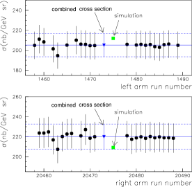
Figure 16: (Color online) Elastic cross section results for the two HRS. The kinematics were $E=1.2$ GeV and $\theta=20^{\circ}$. A systematic error of $6.7\%$ was assigned to each data point, which was dominated by the uncertainty in the target density and the HRS transport functions thesis:zheng .

V.3 $\Delta(1232)$ Transverse Asymmetry

Data on the $\Delta(1232)$ resonance were taken on a transversely polarized target using a beam energy of $1.2$ GeV. The scattered electrons were detected at an angle of $20^{\circ}$ and the central momentum of the spectrometers was set to $0.8$ GeV/c. The transverse asymmetry defined by Eq. (41) was extracted from the raw asymmetry using Eq. (17).

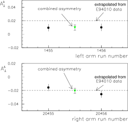
Figure 17: (Color online) Measured raw $\Delta(1232)$ transverse asymmetry, with beam half-wave plate inserted and target spin pointing to the left side of the beamline. The kinematics are $E=1.2$ GeV, $\theta=20^{\circ}$ and $E^{\prime}=0.8$ GeV/c. The dashed lines show the expected value obtained from previous ³He data extrapolated in $Q^{2}$.

A cut in the invariant mass $|W-1232|<20$ (MeV) was used to select $\Delta(1232)$ events. The sign on the right hand side of Eq. (17) depends on the beam half-wave plate status, the spin precession of electrons in the accelerator, the target spin direction, and in which (left or right) HRS the asymmetry is measured. Since data from a previous experiment exp:e94010 in a similar kinematic region showed that $A^{\Delta}_{\parallel}<0$ and $A^{\Delta}_{\perp}>0$ thesis:deur , $A^{\Delta}_{\perp}$ can be used to determine the sign convention of the measured transverse asymmetries. The raw $\Delta(1232)$ transverse asymmetry measured during this experiment was positive on the left HRS, as shown in Fig. 17, with the beam half-wave plate inserted and the target spin pointing to the left side of the beamline. Also shown is the expected value obtained from previous ³He data extrapolated in $Q^{2}$. Similar to the longitudinal configuration, this convention applied to both the $\Delta(1232)$ and DIS measurements.

V.4 False Asymmetry and Background

False asymmetries were checked by measuring the asymmetries from a polarized beam scattering off an unpolarized ¹²C target. The results show that the false asymmetry was less than $2\times 10^{-3}$, which was negligible compared to the statistical uncertainties of the measured ³He asymmetries. To estimate the background from pair production $\gamma\to e^{-}+e^{+}$, the positron yield was measured at $x=0.33$, which is expected to have the highest pair production background. The positron cross section was found to be $\approx 3\%$ of the total cross section at $x=0.33$, and the positron contribution at $x=0.48$ and $x=0.61$ should be even smaller. The effect of pair production asymmetry is negligible compared to the statistical uncertainties of the measured ³He asymmetries and is not corrected for in this analysis.

V.5 DIS Analysis

The longitudinal and transverse asymmetries defined by Eq. (39) and (41) for DIS were extracted from the raw asymmetries as

$$A_{\parallel,\perp} = \pm\frac{A_{raw}}{f_{\mathrm{N}_{2}}P_{b}P_{t}}$$ (20)

where the sign on the right hand side was determined by the procedure described in Sections V.2 and V.3. The N₂ dilution factor, extracted from runs where a reference cell was filled with pure N₂, was found to be $f_{\mathrm{N}_{2}}0.938\pm 0.007$ for all three DIS kinematics.

Radiative corrections were performed for the ³He asymmetries $A_{\parallel}^{{}^{3}\mathrm{He}}$ and $A_{\perp}^{{}^{3}\mathrm{He}}$. We denote by $A^{obs}$ the observed asymmetry, $A^{Born}$ the non-radiated (Born) asymmetry, $\Delta A^{ir}$ the correction due to internal radiation effects and $\Delta A^{er}$ the one due to external radiation effects. One has $A^{Born}=A^{obs}+\Delta A^{ir}+\Delta A^{er}$ for a specific target spin orientation.

Internal corrections were calculated using an improved version of POLRAD 2.0 ana:polrad . External corrections were calculated with a Monte-Carlo simulation based on the procedure first described by Mo and Tsai ana:motsai . Since the theory of radiative corrections is well established ana:motsai , the accuracy of the radiative correction depends mainly on the structure functions used in the procedure. To estimate the uncertainty of both corrections, five different fits ana:f2comfst ; ana:f2nmc92 ; ana:f2nmc95 ; ana:f2pslac94 ; ana:f2phallc02 were used for the unpolarized structure function $F_{2}$ and two fits ana:r1990 ; ana:r1998 were used for the ratio $R$. For the polarized structure function $g_{1}$, in addition to those used in POLRAD 2.0 ana:f2g1sch ; ana:f2g1grsv96 , we fit to world $g_{1}^{p}/F_{1}^{p}$ and $g_{1}^{n}/F_{1}^{n}$ data including the new results from this experiment. Both fits will be presented in Section VI.2. For $g_{2}$ we used both $g_{2}^{WW}$ and an assumption that $g_{2}=0$. The variation in the radiative corrections using the fits listed above was taken as the full uncertainty of the corrections.

Table 4: Total radiation length $X_{0}$ and thickness $d$ of the material traversed by incident (before interaction) and scattered (after interaction) electrons. The cell is made of glass GE180 which has $X_{0}=7.04$ cm and density $\rho=2.77$ g/cm³. The radiation length and thickness after interaction are given by left/right depending on by which HRS the electrons were detected.

$x$	0.33, 0.48	0.61	0.61
$\theta$	35∘	45∘	45∘
Cell	#2	#2	#1
Cell window ($\mu$m)	144	144	132
$X_{0}$ (before)	0.00773	0.00773	0.00758
$d$ (g/cm2, before)	0.23479	0.23479	0.23317
Cell wall (mm)	1.44/1.33	1.44/1.33	1.34/1.43
$X_{0}$ (after)	0.0444/0.0416	0.0376/0.0354	0.0356/0.0374
$d$ (g/cm2, after)	0.9044/0.8506	0.7727/0.7293	0.7336/0.7687

Table 5: Internal radiative corrections to $A_{\parallel}^{{}^{3}\mathrm{He}}$ and $A_{\perp}^{{}^{3}\mathrm{He}}$.

$x$	$\Delta A_{\parallel}^{ir,^{3}\mathrm{He}}$ ($\times 10^{-3}$)	$\Delta A_{\perp}^{ir,^{3}\mathrm{He}}$ ($\times 10^{-3}$)
0.33	-5.77 $\pm$ 0.47	2.66 $\pm$ 0.03
0.48	-3.28 $\pm$ 0.13	1.47 $\pm$ 0.05
0.61	-2.66 $\pm$ 0.15	1.28 $\pm$ 0.07

Table 6: External radiative corrections to $A_{\parallel}^{{}^{3}\mathrm{He}}$ and $A_{\perp}^{{}^{3}\mathrm{He}}$. Errors are from uncertainties in the structure functions and in the cell wall thickness.

$x$	$\Delta A_{\parallel}^{er,^{3}\mathrm{He}}$ ($\times 10^{-3}$)	$\Delta A_{\perp}^{er,^{3}\mathrm{He}}$ ($\times 10^{-3}$)
0.33	-0.67 $\pm$ 0.10	-0.05 $\pm$ 0.11
0.48	-1.16 $\pm$ 0.15	0.80 $\pm$ 0.46
0.61	-0.39 $\pm$ 0.03	0.29 $\pm$ 0.04

For external corrections the uncertainty also includes the contribution from the uncertainty in the target cell wall thickness. The total radiation length and thickness of the material traversed by the scattered electrons are given in Table 4 for each kinematic setting. Results for the internal and external radiative corrections are given in Table 5 and 6, respectively.

By measuring DIS unpolarized cross sections and using the asymmetry results, one can calculate the polarized cross sections and extract $g_{1}$ and $g_{2}$ from Eq. (31) and (32). We used a Monte-Carlo simulation to calculate the expected DIS unpolarized cross sections within the spectrometer acceptance. This simulation included internal and external radiative corrections. The structure functions used in the simulation were from the latest DIS world fits ana:r1998 ; ana:f2nmc95 with the nuclear effects corrected theory:wallyEMC . The radiative corrections from the elastic and quasi-elastic processes were calculated in the peaking approximation ana:peaking using the world proton and neutron form factor data ana:ffpro ; ana:ffneu_dipole ; ana:ffneu_galster . The DIS cross section results agree with the simulation at a level of $10\%$. Since this is not a dedicated cross section experiment, we obtained the values for $g_{1}$ and $g_{2}$ by multiplying our $g_{1}/F_{1}$ and $g_{2}/F_{1}$ results by the world fits for unpolarized structure functions $F_{1}$ ana:f2nmc95 ; ana:r1998 , instead of the $F_{1}$ from this analysis.

V.6 From ³He to Neutron

Properties of protons and neutrons embedded in nuclei are expected to be different from those in free space because of a variety of nuclear effects, including that from spin depolarization, binding and Fermi motion, the off-shell nature of the nucleons, the presence of non-nucleonic degrees of freedom, and nuclear shadowing and antishadowing. A coherent and complete picture of all these effects for the ³He structure function $g_{1}^{{}^{3}\mathrm{He}}$ in the range of $10^{-4}\leq x\leqslant 0.8$ was presented in theory:3Hecmplt . It gives

$$g_{1}^{{}^{3}\mathrm{He}} = P_{n}g_{1}^{n}+2P_{p}g_{1}^{p}-0.014\big{[}{g_{1}^{p}(x)-4g_{1}^{n}(x)}\big{]}$$ (21)

$$+a(x)g_{1}^{n}(x)+b(x)g_{1}^{p}(x)$$

where $P_{n}$($P_{p}$) is the effective polarization of the neutron (proton) inside ³He theory:PnPp_friar . Functions $a(x)$ and $b(x)$ are $Q^{2}$-dependent and represent the nuclear shadowing and antishadowing effects.

From Eq.(38), the asymmetry $A_{1}$ is approximately the ratio of the spin structure function $g_{1}$ and $F_{1}$. Noting that shadowing and antishadowing are not present in the large $x$ region, using Eq. (21) one obtains

$$A_{1}^{n} = \frac{F_{2}^{{}^{3}\mathrm{He}}\big{[}{A_{1}^{{}^{3}\mathrm{He}}}-2\frac{F_{2}^{p}}{F_{2}^{{}^{3}\mathrm{He}}}P_{p}A_{1}^{p}(1-\frac{0.014}{2P_{p}})\big{]}}{P_{n}F_{2}^{n}(1+\frac{0.056}{P_{n}})}~{}.$$ (22)

The two terms $\frac{0.056}{P_{n}}$ and $\frac{0.014}{2P_{p}}$ represent the corrections to $A_{1}^{n}$ associated with the $\Delta(1232)$ component in the ³He wavefunction. Both terms cause $A_{1}^{n}$ to increase in the $x$ range of this experiment, and to turn positive at lower values of $x$ compared to the situation when the effect of the $\Delta(1232)$ is ignored. For $F_{2}^{n}$ and $F_{2}^{{}^{3}\mathrm{He}}$, we used the world proton and deuteron $F_{2}$ data and took into account the EMC effects theory:wallyEMC . We used the world proton asymmetry data for $A_{1}^{p}$. The effective nucleon polarizations $P_{n,p}$ can be calculated using ³He wavefunctions constructed from N-N interactions, and their uncertainties were estimated using various nuclear models theory:PnPp_nogga ; theory:PnPp_friar ; theory:3Heconv ; theory:PnPp_bissey , giving

$$P_{n}=0.86^{+0.036}_{-0.02}~{}~{}\mathrm{and}~{}P_{p}=-0.028^{+0.009}_{-0.004}~{}.$$ (23)

Eq. (22) was also used for extracting $A_{2}^{n}$, $g_{1}^{n}/F_{1}^{n}$ and $g_{2}^{n}/F_{1}^{n}$ from our ³He data. The uncertainty in $A_{1}^{n}$ due to the uncertainties in $F_{2}^{p,d}$, in the correction for EMC effects, in $A_{1}^{p}$ data and in $P_{n,p}$ is given in Table 10. Compared to the convolution approach theory:3Heconv used by previous ³He experiments data:a1ng1n-e142 ; data:a1ng1n-e154 ; data:a1ng1n-hermes , in which only the first two terms on the right hand side of Eq. (21) are present, the values of $A_{1}^{n}$ extracted from Eq. (22) are larger by $(1-2)\%$ in the region $0.2<x<0.7$.

V.7 Resonance Contributions

Since there are a few nucleon resonances with masses above 2 GeV and our measurement at the highest $x$ point has an invariant mass close to $2$ GeV, the effect of possible contributions from baryon resonances were evaluated. This was done by comparing the resonance contribution to $g_{1}^{n}$ with that to $F_{1}^{n}$. For our kinematics at $x=0.6$, data on the unpolarized structure function $F_{2}$ and $R$ data:f2p-hallc show that the resonance contribution to $F_{1}$ is less than $5\%$. The resonance asymmetry was estimated using the MAID model theory:maid and was found to be approximately $0.10$ at $W=1.7$ (GeV). Since the resonance structure is more evident at smaller $W$, we took this value as an upper limit of the contribution at $W=2$ (GeV). The resonance contribution to our $A_{1}^{n}$ and $g_{1}^{n}/F_{1}^{n}$ results at $x=0.6$ were then estimated to be at most $0.008$, which is negligible compared to their statistical errors.

VI RESULTS

VI.1 ³He Results

Results of the electron asymmetries for $\vec{e}-^{3}\vec{\mathrm{He}}$ scattering, $A_{\parallel}^{{}^{3}\mathrm{He}}$ and $A_{\perp}^{{}^{3}\mathrm{He}}$, the virtual photon asymmetries $A_{1}^{{}^{3}\mathrm{He}}$ and $A_{2}^{{}^{3}\mathrm{He}}$, structure function ratios $g_{1}^{{}^{3}\mathrm{He}}/F_{1}^{{}^{3}\mathrm{He}}$ and $g_{2}^{{}^{3}\mathrm{He}}/F_{1}^{{}^{3}\mathrm{He}}$ and polarized structure functions $g_{1}^{{}^{3}\mathrm{He}}$ and $g_{2}^{{}^{3}\mathrm{He}}$ are given in Table 7. Results for $g_{1,2}^{{}^{3}\mathrm{He}}$ were obtained by multiplying the $g_{1,2}^{{}^{3}\mathrm{He}}/F_{1}^{{}^{3}\mathrm{He}}$ results by the unpolarized structure function $F_{1}^{{}^{3}\mathrm{He}}$, which were calculated using the latest world fits of DIS data ana:r1998 ; ana:f2nmc95 and with nuclear effects corrected theory:wallyEMC . Results for $A_{1}^{{}^{3}\mathrm{He}}$ and $g_{1}^{{}^{3}\mathrm{He}}$ are shown in Fig. 18 along with SLAC data:a1ng1n-e142 ; data:a1heg1he-e154 and HERMES data:hermes_dqq data.

Figure 18: Results for the ³He asymmetry $A_{1}^{{}^{3}\mathrm{He}}$ and the structure functions $g_{1}^{{}^{3}\mathrm{He}}$ as a function of $x$, along with previous data from SLAC data:a1ng1n-e142 ; data:a1heg1he-e154 and HERMES data:hermes_dqq . Error bars of the results from this work include both statistical and systematic uncertainties.

Table 7: Results for ³He asymmetries $A_{1}^{{}^{3}\mathrm{He}}$ and $A_{2}^{{}^{3}\mathrm{He}}$, structure function ratios $g_{1}^{{}^{3}\mathrm{He}}/F_{1}^{{}^{3}\mathrm{He}}$ and $g_{2}^{{}^{3}\mathrm{He}}/F_{1}^{{}^{3}\mathrm{He}}$, and polarized structure functions $g_{1}^{{}^{3}\mathrm{He}}$ and $g_{2}^{{}^{3}\mathrm{He}}$. Errors are given as $\pm$ statistical $\pm$ systematic.

$\langle x\rangle$	0.33	0.47	0.60
$\langle Q^{2}\rangle$ (GeV/c)2	2.71	3.52	4.83
$A_{\parallel}^{{}^{3}\mathrm{He}}$	$-0.020\pm 0.005\pm 0.001$	$-0.012\pm 0.005\pm 0.000$	$0.007\pm 0.007\pm 0.001$
$A_{\perp}^{{}^{3}\mathrm{He}}$	$0.000\pm 0.010\pm 0.000$	$0.016\pm 0.008\pm 0.001$	$-0.010\pm 0.016\pm 0.001$
$A_{1}^{{}^{3}\mathrm{He}}$	$-0.024\pm 0.006\pm 0.001$	$-0.019\pm 0.006\pm 0.001$	$0.010\pm 0.009\pm 0.001$
$A_{2}^{{}^{3}\mathrm{He}}$	$-0.004\pm 0.014\pm 0.001$	$0.020\pm 0.012\pm 0.001$	$-0.013\pm 0.023\pm 0.001$
$g_{1}^{{}^{3}\mathrm{He}}/F_{1}^{{}^{3}\mathrm{He}}$	$-0.022\pm 0.005\pm 0.001$	$-0.008\pm 0.008\pm 0.001$	$0.003\pm 0.009\pm 0.001$
$g_{2}^{{}^{3}\mathrm{He}}/F_{1}^{{}^{3}\mathrm{He}}$	$0.010\pm 0.036\pm 0.002$	$0.050\pm 0.022\pm 0.003$	$-0.028\pm 0.038\pm 0.002$
$g_{1}^{{}^{3}\mathrm{He}}$	$-0.024\pm 0.006\pm 0.001$	$-0.004\pm 0.004\pm 0.000$	$0.001\pm 0.002\pm 0.000$
$g_{2}^{{}^{3}\mathrm{He}}$	$0.011\pm 0.039\pm 0.001$	$0.026\pm 0.012\pm 0.002$	$-0.006\pm 0.009\pm 0.001$

VI.2 Neutron Results

Results for the neutron asymmetries $A_{1}^{n}$ and $A_{2}^{n}$, structure function ratios $g_{1}^{n}/F_{1}^{n}$ and $g_{2}^{n}/F_{1}^{n}$ and polarized structure functions $g_{1}^{n}$ and $g_{2}^{n}$ are given in Table 8.

Table 8: Results for the asymmetries and spin structure functions for the neutron. Errors are given as $\pm$statistical $\pm$systematic.

$\langle x\rangle$	0.33	0.47	0.60
$\langle Q^{2}\rangle$ (GeV/c)2	2.71	3.52	4.83
$A_{1}^{n}$	$-0.048\pm 0.024^{+0.015}_{-0.016}$	$-0.006\pm 0.027^{+0.019}_{-0.019}$	$0.175\pm 0.048^{+0.026}_{-0.028}$
$A_{2}^{n}$	$-0.004\pm 0.063^{+0.005}_{-0.005}$	$0.117\pm 0.055^{+0.012}_{-0.021}$	$-0.034\pm 0.124^{+0.014}_{-0.014}$
$g_{1}^{n}/F_{1}^{n}$	$-0.043\pm 0.022^{+0.009}_{-0.009}$	$0.040\pm 0.035^{+0.011}_{-0.011}$	$0.124\pm 0.045^{+0.016}_{-0.017}$
$g_{2}^{n}/F_{1}^{n}$	$0.034\pm 0.153^{+0.010}_{-0.010}$	$0.207\pm 0.103^{+0.022}_{-0.021}$	$-0.190\pm 0.204^{+0.027}_{-0.027}$
$g_{1}^{n}$	$-0.012\pm 0.006^{+0.003}_{-0.003}$	$0.005\pm 0.004^{+0.001}_{-0.001}$	$0.006\pm 0.002^{+0.001}_{-0.001}$
$g_{2}^{n}$	$0.009\pm 0.043^{+0.003}_{-0.003}$	$0.026\pm 0.013^{+0.003}_{-0.003}$	$-0.009\pm 0.009^{+0.001}_{-0.001}$

The $A_{1}^{n}$, $g_{1}^{n}/F_{1}^{n}$ and $g_{1}^{n}$ results are shown in Fig. 19, 20 and 21, respectively. In the region of $x>0.4$, our results have improved the world data precision by about an order of magnitude, and will provide valuable inputs to parton distribution function (PDF) parameterizations. Our data at $x=0.33$ are in good agreement with previous world data. For the $A_{1}^{n}$ results, this is the first time that the data show a clear trend that $A_{1}^{n}$ turns to positive values at large $x$. As $x$ increases, the agreement between the data and the predictions from the constituent quark models (CQM) becomes better. This is within the expectation since the CQM is more likely to work in the valence quark region. It also indicates that $A_{1}^{n}$ will go to higher values at $x>0.6$. However, the trend of the $A_{1}^{n}$ results does not agree with the BBS and LSS(BBS) parameterizations, which are from leading-order pQCD analyses based on hadron helicity conservation (HHC). This indicates that there might be problem in the assumption that quarks have zero orbital angular momentum which is used by HHC.

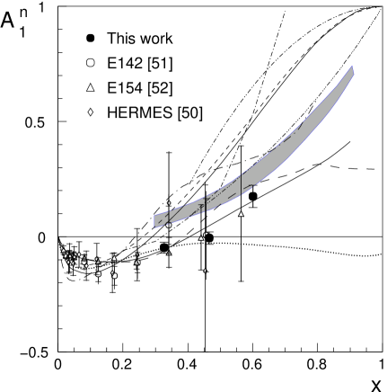
Figure 19: Our $A_{1}^{n}$ results along with theoretical predictions and previous world data obtained from polarized ³He targets data:a1ng1n-e142 ; data:a1ng1n-e154 ; data:a1ng1n-hermes . Curves: predictions of $A_{1}^{n}$ from SU(6) symmetry ($x$ axis at zero) theory:su6close , constituent quark model (shaded band) theory:cqm , statistical model at $Q^{2}=4$ (GeV/c)² (long-dashed) theory:stat , quark-hadron duality using two different SU(6) breaking mechanisms (dash-dot-dotted and dash-dot-dot-dotted), and non-meson cloudy bag model (dash-dotted) theory:bag ; predictions of ${g_{1}^{n}}/{F_{1}^{n}}$ from pQCD HHC based BBS parameterization at $Q^{2}=4$ (GeV/c)² (higher solid) theory:bbs and LSS(BBS) parameterization at $Q^{2}=4$ (GeV/c)² (dashed) theory:lssbbs , LSS 2001 NLO polarized parton densities at $Q^{2}=5$ (GeV/c)² (lower solid) theory:lss2001 and chiral soliton models theory:chi_weigel at $Q^{2}=3$ (GeV/c)² (long dash-dotted) and theory:chi_waka at $Q^{2}=4.8$ (GeV/c)² (dotted).

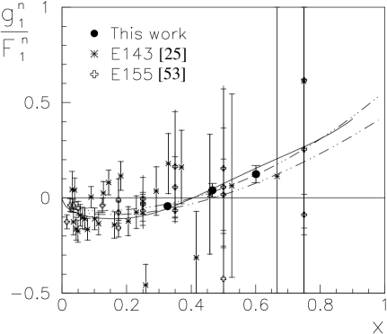
Figure 20: Results for $g_{1}^{n}/F_{1}^{n}$ along with previous world data from SLAC data:a1pa1n-e143 ; data:g1pg1n-e155 . The curves are the prediction for $g_{1}^{n}/F_{1}^{n}$ from the LSS 2001 NLO polarized parton densities at $Q^{2}=5$ (GeV/c)² theory:lss2001 , the E155 experimental fit at $Q^{2}=5$ (GeV/c)² (long dash-dot-dotted) data:g1pg1n-e155 and the new fit as described in the text (long dash-dot-dot-dotted).

Figure 21: Results for $g_{1}^{n}$ along with previous world data from SLAC data:a1ng1n-e142 ; data:a1ng1n-e154 ; data:g1pg1n-e155 and HERMES data:a1ng1n-hermes .

The sources for the experimental systematic uncertainties are listed in Table 9.

Table 9: Experimental systematic errors for the $A_{1}^{n}$ result.

source	error
Beam energy $E_{b}$	${\Delta E_{b}}/{E_{b}}<5\times 10^{-4}$
HRS central momentum $p_{0}$	${\Delta E_{e}}/{E_{e}}<5\times 10^{-4}$ technote:HRSgamma
HRS central angle $\theta_{0}$	$\Delta\theta_{0}<0.1^{\circ}$ exp:hallATN02-032
Beam polarization $P_{b}$	${\Delta P_{b}}/{P_{b}}<3\%$
Target polarization $P_{t}$	${\Delta P_{t}}/{P_{t}}<4\%$
Target spin direction $\alpha_{t}$	$\Delta\alpha_{t}<1^{\circ}$

Systematic uncertainties for the $A_{1}^{n}$ results include that from experimental systematic errors, uncertainties in internal radiative corrections $\Delta A_{1}^{n,ir}$ and external radiative corrections $\Delta A_{1}^{n,er}$ as derived from the values in Tables 5 and 6, and that from nuclear corrections as described in Section V.6. Table 10 gives these systematic uncertainties for the $A_{1}^{n}$ results along with their statistical uncertainties. The total uncertainties are dominated by the statistical uncertainties.

Table 10: Total uncertainties for $A_{1}^{n}$.

$\langle x\rangle$	0.33	0.47	0.60
Statistics	0.024	0.027	0.048
Experimental syst.	0.004	0.003	0.004
$\Delta A_{1}^{n,ir}$	0.012	0.013	0.015
$\Delta A_{1}^{n,er}$	0.002	0.002	0.003
$F_{2}^{p}$, $F_{2}^{d}$	0.006	0.008	${}^{+0.005}_{-0.010}$
EMC effect	0.001	0.000	0.009
$A_{1}^{p}$	0.001	0.005	0.011
$P_{n}$, $P_{p}$	${}^{+0.005}_{-0.012}$	${}^{+0.009}_{-0.020}$	${}^{+0.018}_{-0.037}$

We used five functional forms, $x^{\alpha}P_{n}(x)(1+\beta/Q^{2})$, to fit our $g_{1}^{n}/F_{1}^{n}$ results combined with data from previous experiments data:a1pa1n-e143 ; data:g1pg1n-e155 . Here $P_{n}$ is the $n^{th}$-order polynomial, $n=1,2$ for a finite $\alpha$ or $n=1,2,3$ if $\alpha$ is fixed to be $0$. The total number of parameters is limited to $\leqslant 5$. For the $Q^{2}$-dependence of $g_{1}/F_{1}$, we used a term $1+\beta/Q^{2}$ as in the E155 experimental fit data:g1pg1n-e155 . No constraints were imposed on the fit concerning the behavior of $g_{1}/F_{1}$ as $x\to 1$. The function which gives the smallest $\chi^{2}$ value is $g_{1}^{n}/F_{1}^{n}=(a+bx+cx^{2})(1+\beta/Q^{2})$. The new fit is shown in Fig. 20. Results for the fit parameters are given in Table 11 and the covariance error matrix is

$${\epsilon}=\left[\begin{array}[]{cccc}1.000&-0.737&0.148&0.960\\ -0.737&1.000&-0.752&-0.581\\ 0.148&-0.752&1.000&-0.039\\ 0.960&-0.581&-0.039&1.000\end{array}\right]~{}.$$

Table 11: Result of the fit $g_{1}^{n}/F_{1}^{n}=(a+bx+cx^{2})(1+\beta/Q^{2})$.

$a=-0.049\pm 0.052$

$b=-0.162\pm 0.217$

$c=0.698\pm 0.345$

$\beta=0.751\pm 2.174$

Similar fits were performed to the proton world data data:g1p-hermes ; data:a1pa1n-e143 ; data:g1pg1n-e155 and function $g_{1}^{p}/F_{1}^{p}=x^{\alpha}(a+bx)(1+\beta/Q^{2})$ was found to give the smallest $\chi^{2}$ value. The new fit is shown in Fig. 2 of Section II.7. Results for the fit parameters are given in Table 12 and the covariance error matrix is

$${\epsilon}=\left[\begin{array}[]{cccc}1.000&0.908&-0.851&0.723\\ 0.908&1.000&-0.967&0.401\\ -0.851&-0.967&1.000&-0.369\\ 0.723&0.401&-0.369&1.000\end{array}\right]~{}.$$

Table 12: Result of the fit $g_{1}^{p}/F_{1}^{p}=x^{\alpha}(a+bx)(1+\beta/Q^{2})$.

$\alpha=0.813\pm 0.049$

$a=1.231\pm 0.122$

$b=-0.413\pm 0.216$

$\beta=0.030\pm 0.124$

Figures 22 and 23 show the results for $A_{2}^{n}$ and $xg_{2}^{n}$, respectively. The precision of our data is comparable to the data from E155x experiment at SLAC data:e155x , which is so far the only experiment dedicated to measuring $g_{2}$ with published results.

To evaluate the matrix element $d_{2}^{n}$, we combined our $g_{2}^{n}$ results with the E155x data data:e155x . The average $Q^{2}$ of the E155x data set is about $5$ (GeV/c)². Following a similar procedure as used in Ref. data:e155x , we assumed that $\bar{g}_{2}(x,Q^{2})$ is independent of $Q^{2}$ and $\bar{g}_{2}\propto(1-x)^{m}$ with $m=2$ or $3$ for $x\mathrel{\raise 1.29167pt\hbox{$>$}\mkern-14.0mu\lower 3.01385pt\hbox{$\sim$}}0.78$ beyond the measured region of both experiments. We obtained from Eq. (6)

$$d_{2}^{n} = 0.0062\pm 0.0028~{}.$$ (24)

Compared to the value published previously data:e155x , the uncertainty on $d_{2}^{n}$ has been improved by about a factor of two. The large decrease in uncertainty despite the small number of our data points arises from the $x^{2}$ weighting of the integral which emphasizes the large $x$ kinematics. The uncertainties on the integrand has been improved in the region $x>0.4$ due to our $g_{2}^{n}$ results at the two higher $x$ points being more precise than that of E155x. While a negative value was predicted by lattice QCD theory:d2lattice and most other models theory:d2bag ; theory:d2QCDSR ; theory:d2chi , the new result for $d_{2}^{n}$ suggests that the higher twist contribution is positive.

Figure 22: Results for $A_{2}^{n}$ along with the best previous world data data:e155x . The curve gives the twist-2 contribution at $Q^{2}=4$ (GeV/c)² calculated using the E155 experimental fit data:g1pg1n-e155 and $g_{2}^{WW}$ of Eq. (5).

Figure 23: Results for $xg_{2}^{n}$ along with the best previous world data data:e155x . The curve gives the twist-2 contribution at $Q^{2}=4$ (GeV/c)² calculated using the E155 experimental fit data:g1pg1n-e155 and $g_{2}^{WW}$ of Eq. (5).

VI.3 Flavor Decomposition using the Quark-Parton Model

Assuming the strange quark distributions $s(x)$, $\bar{s}(x)$, $\Delta s(x)$ and $\Delta\bar{s}(x)$ to be small in the region $x>0.3$, and ignoring any $Q^{2}$-dependence of the ratio of structure functions, one can extract polarized quark distribution functions based on the quark-parton model as

$${{\frac{\Delta u+\Delta\bar{u}}{u+\bar{u}}}} = \frac{4g_{1}^{p}(4+\mathit{R^{du}})}{15F_{1}^{p}}-\frac{g_{1}^{n}(1+4\mathit{R^{du}})}{15F_{1}^{n}}~{}$$ (25)

and

$${{\frac{\Delta d+\Delta\bar{d}}{d+\bar{d}}}} = \frac{4g_{1}^{n}(1+4\mathit{R^{du}})}{15F_{1}^{n}\mathit{R^{du}}}-\frac{g_{1}^{p}(4+\mathit{R^{du}})}{15F_{1}^{p}\mathit{R^{du}}}~{},$$ (26)

with $\mathit{R^{du}}\equiv({d+\bar{d}})/({u+\bar{u}})$. Results for $({\Delta u+\Delta\bar{u}})/(u+$ $\bar{u})$ and $({\Delta d+\Delta\bar{d}})/({d+\bar{d}})$ are given in Table 13. As inputs we used our own results for $g_{1}^{n}/F_{1}^{n}$, the world data on $g_{1}^{p}/F_{1}^{p}$ thesis:zheng , and the ratio $\mathit{R^{du}}$ extracted from proton and deuteron unpolarized structure function data theory:duratio . In a similar manner as for Eq.(25) and (26) and ignoring nuclear effects, one can also add the world data on $g_{1}^{{}^{2}\mathrm{H}}/F_{1}^{{}^{2}\mathrm{H}}$ to the fitted data set and extract these polarized quark distributions. The results are, however, consistent with those given in Table 13 and have very similar error bars because the data on the deuteron in general have poorer precision than the data on the proton and the neutron data from this experiment. The results presented here have changed compared to the values published previously in Ref. A1nPRL due to an error discovered in our fitting of $\mathit{R^{du}}$ from Ref. theory:duratio . The analysis procedure is consistent with what was used in Ref. A1nPRL .

Table 13: Results for the polarized quark distributions. The three uncertainties are those due to the $g_{1}^{n}/F_{1}^{n}$ statistical error, $g_{1}^{n}/F_{1}^{n}$ systematic uncertainty and the uncertainties of the $g_{1}^{p}/F_{1}^{p}$ data, the $\mathit{R^{du}}$ fit and the correction for $s$ and $c$ quark contributions.

$\langle x\rangle$	$({\Delta u+\Delta\bar{u}})/({u+\bar{u}})$	$({\Delta d+\Delta\bar{d}})/({d+\bar{d}})$
$0.33$	$0.545\pm 0.004\pm 0.002_{-0.025}^{+0.024}$	$-0.352\pm 0.035\pm 0.014_{-0.031}^{+0.017}$
$0.47$	$0.649\pm 0.006\pm 0.002_{-0.058}^{+0.058}$	$-0.393\pm 0.063\pm 0.020_{-0.049}^{+0.041}$
$0.60$	$0.728\pm 0.006\pm 0.002_{-0.114}^{+0.114}$	$-0.440\pm 0.092\pm 0.035_{-0.142}^{+0.107}$

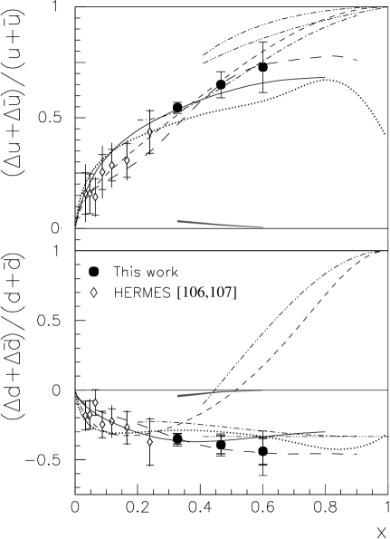
Figure 24: Results for $({\Delta u+\Delta\bar{u}})/({u+\bar{u}})$ and $({\Delta d+\Delta\bar{d}})/({d+\bar{d}})$ in the quark-parton model, compared with semi-inclusive data from HERMES data:hermes_newdqq and CTEQ unpolarized PDF theory:cteq as described in the text, the RCQM predictions (dash-dotted) theory:cqm , predictions from LSS 2001 NLO polarized parton densities at $Q^{2}=5$ (GeV/c)² (solid) theory:lss2001 , the statistical model at $Q^{2}=4$ (GeV/c)² (long-dashed) theory:stat , the pQCD-based predictions with the HHC constraint (dashed) theory:lssbbs , the duality model using two different SU(6) breaking mechanisms (dash-dot-dotted and dash-dot-dot-dotted) theory:dual_new , and predictions from chiral soliton model at $Q^{2}=4.8$ (GeV/c)² (dotted) theory:chi_waka . The error bars of our data include the uncertainties given in Table 13. The shaded band near the horizontal axis shows the difference between $\Delta q_{V}/q_{V}$ and $(\Delta q+\Delta\bar{q})/(q+\bar{q})$ that needs to be added to the data when comparing with the RCQM calculation.

Figure 24 shows our results along with semi-inclusive data on $(\Delta q+\Delta\bar{q})/(q+\bar{q})$ obtained from recent results for $\Delta q$ and $\Delta\bar{q}$ data:hermes_newdqq by the HERMES collaboration, and the CTEQ6M unpolarized PDF theory:cteq . To estimate the effect of the $s$ and $\bar{s}$ contributions, we used two unpolarized PDF sets, CTEQ6M theory:cteq and MRST2001 theory:mrst , and three polarized PDF sets, AAC2003 theory:aac03_polpdf , BB2002 theory:bb_polpdf and GRSV2000 theory:grsv2000_polpdf . For $c$ and $\bar{c}$ contributions we used the two unpolarized PDF sets theory:cteq ; theory:mrst and the positivity conditions that $|{\Delta c/c}|\leqslant~{}1$ and $|{\Delta\bar{c}/\bar{c}}|\leqslant~{}1$. To compare with the RCQM predictions, which are given for valence quarks, the difference between $\Delta q_{V}/q_{V}$ and $(\Delta q+\Delta\bar{q})/(q+\bar{q})$ was estimated using the two unpolarized PDF sets theory:cteq ; theory:mrst and the three polarized PDF sets theory:aac03_polpdf ; theory:bb_polpdf ; theory:grsv2000_polpdf and is shown as the shaded band near the horizontal axis of Fig. 24. Here $q_{V}$($\Delta q_{V}$) is the unpolarized (polarized) valence quark distribution for $u$ or $d$ quark. Results shown in Fig. 24 agree well with the predictions from the RCQM theory:cqm and the LSS 2001 NLO polarized parton densities theory:lss2001 . The results agree reasonably well with the statistical model calculation theory:stat . But results for the $d$ quark do not agree with the predictions from the leading-order pQCD LSS(BBS) parameterization theory:lssbbs assuming hadron helicity conservation.

VII CONCLUSIONS

We have presented precise data on the neutron spin asymmetry $A_{1}^{n}$ and the structure function ratio $g_{1}^{n}/F_{1}^{n}$ in the deep inelastic region at large $x$ obtained from a polarized ³He target. These results will provide valuable inputs to the QCD parameterizations of parton densities. The new data show a clear trend that $A_{1}^{n}$ becomes positive at large $x$. Our results for $A_{1}^{n}$ agree with the LSS 2001 NLO QCD fit to the previous data and the trend of the $x$-dependence of $A_{1}^{n}$ agrees with the hyperfine-perturbed RCQM predictions. Data on the transverse asymmetry and structure function $A_{2}^{n}$ and $g_{2}^{n}$ were also obtained with a precision comparable to the best previous world data in this kinematic region. Combined with previous world data, the matrix element $d_{2}^{n}$ was evaluated and the new value differs from zero by more than two standard deviations. This result suggests that the higher twist contribution is positive. Combined with the world proton data, the polarized quark distributions $(\Delta u+\Delta\bar{u})/(u+\bar{u})$ and $(\Delta d+\Delta\bar{d})/(d+\bar{d})$ were extracted based on the quark parton model. While results for $(\Delta u+\Delta\bar{u})/(u+\bar{u})$ agree well with predictions from various models and fits to the previous data, results for $(\Delta d+\Delta\bar{d})/(d+\bar{d})$ agree with the predictions from RCQM and from the LSS 2001 fit, but do not agree with leading order pQCD predictions that use hadron helicity conservation. Since hadron helicity conservation is based on the assumption that quarks have negligible orbital angular momentum, the new results suggest that the quark orbital angular momentum, or other effects beyond leading-order pQCD, may play an important role in this kinematic region.

Appendix A Formalism for Electron Deep Inelastic Scattering

The fundamental quark and gluon structure of strongly interacting matter is studied primarily through experiments that emphasize hard scattering from the quarks and gluons at sufficiently high energies. One important way of probing the distribution of quarks and antiquarks inside the nucleon is electron scattering, where an electron scatters from a single quark or antiquark inside the target nucleon and transfers a large fraction of its energy and momentum via exchanged photons. In the single photon exchange approximation, the electron interacts with the target nucleon via only one photon, as shown in Fig. 25 book:thomas&weise , and probes the quark structure of the nucleon with a spatial resolution determined by the four momentum transfer squared of the photon $Q^{2}\equiv-q^{2}$. Moreover, if a polarized electron beam and a polarized target are used, the spin structure of the nucleon becomes accessible.

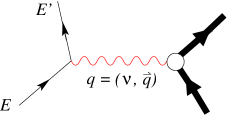
Figure 25: (Color online) Electron scattering in the one-photon exchange approximation.

In the following we denote the incident electron energy by $E$, the energy of the scattered electron by $E^{\prime}$ thus the energy transfer of the photon is $\nu=E-E^{\prime}$, and the three-momentum transfer from the electron to the target nucleus by $\vec{q}$.

A.1 Structure Functions

In the case of unpolarized electrons scattering off an unpolarized target, the differential cross-section for detecting the outgoing electron in a solid angle $\mathrm{d}\Omega$ and an energy range ($E^{\prime}$, $E^{\prime}+\mathrm{d}E^{\prime}$) in the laboratory frame can be written as

$$\frac{\mathrm{d}^{2}\sigma}{\mathrm{d}\Omega\mathrm{d}E^{\prime}}= \Big{(}\frac{\mathrm{d}\sigma}{\mathrm{d}\Omega}\Big{)}_{Mott}\cdot$$ (27)

$$\Big{[}\frac{1}{\nu}F_{2}(x,Q^{2})+\frac{2}{M}F_{1}(x,Q^{2})\tan^{2}\frac{\theta}{2}\Big{]}~{},$$

where $\theta$ is the scattering angle of the electron in the laboratory frame. The four momentum transfer $Q^{2}$ is given by

$$Q^{2} = 4EE^{\prime}\sin^{2}\frac{\theta}{2}~{},$$ (28)

and the Mott cross section,

$${\Big{(}\frac{\mathrm{d}\sigma}{\mathrm{d}\Omega}\Big{)}}_{Mott} = \frac{\alpha^{2}\cos^{2}{\frac{\theta}{2}}}{4E^{2}\sin^{4}{\frac{\theta}{2}}}=\frac{\alpha^{2}\cos^{2}{\frac{\theta}{2}}}{Q^{4}}\frac{E^{\prime}}{E}~{}$$ (29)

with $\alpha$ the fine structure constant, is the cross section for scattering relativistic electrons from a spin-0 point-like infinitely heavy target. $F_{1}(x,Q^{2})$ and $F_{2}(x,Q^{2})$ are the unpolarized structure functions of the target, which are related to each other as

$$F_{1}(x,Q^{2}) = \frac{F_{2}(x,Q^{2})(1+\gamma^{2})}{2x\Big{(}1+R(x,Q^{2})\Big{)}}$$ (30)

with $\gamma^{2}={(2Mx)^{2}}/{Q^{2}}$. Here $R$ is defined as $R\equiv{\sigma_{L}}/{\sigma_{T}}$ with $\sigma_{L}$ and $\sigma_{T}$ the longitudinal and transverse virtual photon cross sections, which can also be expressed in terms of $F_{1}$ and $F_{2}$.

Note that for a nuclear target, there exists an alternative per nucleon definition (e.g. as used in Ref. ana:f2nmc95 ) which is $1/A$ times the definition used in this paper, here $A$ is the number of nucleons inside the target nucleus.

A review of doubly polarized DIS was given in Ref. theory:disreview . When the incident electrons are longitudinally polarized, the cross section difference between scattering off a target with its nuclear (or nucleon) spins aligned anti-parallel and parallel to the incident electron momentum is

$$\frac{\mathrm{d}^{2}\sigma_{\uparrow\Downarrow}}{\mathrm{d}\Omega\mathrm{d}E^{\prime}}-\frac{\mathrm{d}^{2}\sigma_{\uparrow\Uparrow}}{\mathrm{d}\Omega\mathrm{d}E^{\prime}}=\frac{4\alpha^{2}E^{\prime}}{\nu EQ^{2}}$$

$$\times\Big{[}{(E+E^{\prime}\cos{\theta}){{g_{1}(x,Q^{2})}}-2Mx{{g_{2}(x,Q^{2})}}}\Big{]}~{}.$$ (31)

where $g_{1}(x,Q^{2})$ and $g_{2}(x,Q^{2})$ are the polarized structure functions. If the target nucleons are transversely polarized, then the cross section difference is given by

$$\frac{\mathrm{d}^{2}\sigma_{\uparrow\Rightarrow}}{\mathrm{d}\Omega\mathrm{d}E^{\prime}}- \frac{\mathrm{d}^{2}\sigma_{\uparrow\Leftarrow}}{\mathrm{d}\Omega\mathrm{d}E^{\prime}}=\frac{4\alpha^{2}E^{{}^{\prime}2}}{\nu EQ^{2}}\sin{\theta}$$ (32)

$$\times\Big{[}{{g_{1}(x,Q^{2})}}+\frac{2E}{\nu}{{g_{2}(x,Q^{2})}}\Big{]}~{}.$$

A.2 Bjorken Scaling and Its Violation

A remarkable feature of the structure functions $F_{1}$, $F_{2}$, $g_{1}$ and $g_{2}$ is their scaling behavior. In the Bjorken limit theory:bjorken ($Q^{2}\to\infty$ and $\nu\to\infty$ at a fixed value of $x$), the structure functions become independent of $Q^{2}$ data:slac-bjscaling . Moreover, in this limit $\sigma_{L}$ vanishes book:thomas&weise , hence $R=0$ and Eq. (30) reduces to $F_{2}(x)=2xF_{1}(x)$, known as the Callan-Gross relation theory:Callan-Gross .

At finite $Q^{2}$, the scaling of structure functions is violated due to the radiation of gluons by both initial and scattered quarks. These gluon radiative corrections cause a logarithmic $Q^{2}$-dependence to the structure functions, which has been verified by experimental data exp:pdg and can be precisely calculated in pQCD using the Dokshitzer-Gribov-Lipatov-Altarelli-Parisi (DGLAP) evolution equations theory:dglap .

A.3 From Bjorken Limit to Finite $Q^{2}$ using the Operator Product Expansion

In order to calculate observables at finite values of $Q^{2}$, a method called the Operator Product Expansion (OPE) theory:ope can be applied to DIS which can separate the non-perturbative part of an observable from its perturbative part. In the OPE, whether an operator is perturbative or not is characterized by the “twist” of the operator. At large $Q^{2}$ the leading twist $t=2$ term dominates, while at small $Q^{2}$ higher-twist operators need to be taken into account, which are sensitive to interactions beyond the quark-parton model, e.g., quark-gluon and quark-quark correlations theory:ope-g2 .

A.4 Virtual Photon-Nucleon Asymmetries

Virtual photon asymmetries are defined in terms of a helicity decomposition of the virtual photon absorption cross sections theory:drechsel . For the absorption of circularly polarized virtual photons with helicity $\pm 1$ by longitudinally polarized nucleons, the longitudinal asymmetry $A_{1}$ is defined as

$$A_{1}(x,Q^{2}) \equiv \frac{\sigma_{{1}/{2}}-\sigma_{{3}/{2}}}{\sigma_{{1}/{2}}+\sigma_{{3}/{2}}}~{},$$ (33)

where $\sigma_{1/2(3/2)}$ is the total virtual photo-absorption cross section for the nucleon with a projection of $1/2(3/2)$ for the total spin along the direction of photon momentum.

$A_{2}$ is a virtual photon asymmetry given by

$$A_{2}(x,Q^{2}) \equiv \frac{2\sigma_{LT}}{\sigma_{{1}/{2}}+\sigma_{{3}/{2}}}~{}.$$ (34)

where $\sigma_{LT}$ describes the interference between transverse and longitudinal virtual photon-nucleon amplitudes. Because of the positivity limit, $A_{2}$ is usually small in the DIS region and it has an upper bound given by theory:a2soffer

$$A_{2}(x,Q^{2})\leqslant\sqrt{\frac{R}{2}\Big{[}1+A_{1}(x,Q^{2})\Big{]}}~{}.$$ (35)

These two virtual photon asymmetries, depending in general on $x$ and $Q^{2}$, are related to the nucleon structure functions $g_{1}(x,Q^{2})$, $g_{2}(x,Q^{2})$ and $F_{1}(x,Q^{2})$ via

$$A_{1}(x,Q^{2}) = \frac{g_{1}(x,Q^{2})-\gamma^{2}g_{2}(x,Q^{2})}{F_{1}(x,Q^{2})}~{}$$ (36)

and

$$A_{2}(x,Q^{2}) = \frac{\gamma\Big{[}g_{1}(x,Q^{2})+g_{2}(x,Q^{2})\Big{]}}{F_{1}(x,Q^{2})}~{}.$$ (37)

At high $Q^{2}$, one has $\gamma^{2}\ll 1$ and

$$A_{1}(x,Q^{2}) \approx \frac{g_{1}(x,Q^{2})}{F_{1}(x,Q^{2})}~{}.$$ (38)

In QCD the asymmetry $A_{1}$ is expected to have less $Q^{2}$-dependence than the structure functions themselves because of the similar leading order $Q^{2}$-evolution behavior of $g_{1}(x,Q^{2})$ and $F_{1}(x,Q^{2})$. Existing data on the proton and the neutron asymmetries $A_{1}^{p}$ and $A_{1}^{n}$ indeed show little $Q^{2}$-dependence data:g1pg1n-e155 .

A.5 Electron Asymmetries

In an inclusive experiment covering a large range of excitation energies the virtual photon momentum direction changes frequently, and it is usually more practical to align the target spin longitudinally or transversely to the incident electron direction than to the momentum of the virtual photon. The virtual photon asymmetries can be related to the measured electron asymmetries through polarization factors, kinematic variables and the ratio $R$ defined in Section A.1. The longitudinal electron asymmetry is defined by exp:e080

$$A_{\parallel} \equiv \frac{\sigma_{\downarrow\Uparrow}-\sigma_{\uparrow\Uparrow}}{\sigma_{\downarrow\Uparrow}+\sigma_{\uparrow\Uparrow}}$$ (39)

$$= \frac{(1-\epsilon)M^{3}}{(1-\epsilon R)\nu F_{1}}\Big{[}(E+E^{\prime}\cos\theta)g_{1}-\frac{Q^{2}}{\nu}g_{2}\Big{]}~{},$$

where $\sigma_{\downarrow\Uparrow}$($\sigma_{\uparrow\Uparrow}$) is the cross section of scattering off a longitudinally polarized target, with the incident electron spin aligned anti-parallel (parallel) to the target spin, and $\epsilon$ is the magnitude of the virtual photon’s longitudinal polarization:

$$\epsilon = \Big{[}1+2(1+1/\gamma^{2})\tan^{2}(\theta/2)\Big{]}^{-1}~{}.$$ (40)

Similarly the transverse electron asymmetry is defined for a target polarized perpendicular to the beam direction as

$$A_{\perp} \equiv \frac{\sigma_{\downarrow\Rightarrow}-\sigma_{\uparrow\Rightarrow}}{\sigma_{\downarrow\Rightarrow}+\sigma_{\uparrow\Rightarrow}}$$ (41)

$$= \frac{(1-\epsilon)E^{\prime}M^{3}}{(1-\epsilon R)\nu F_{1}}\Big{[}g_{1}+\frac{2E}{\nu}g_{2}\Big{]}\cos\theta~{},~{}$$

where $\sigma_{\downarrow\Rightarrow}$($\sigma_{\uparrow\Rightarrow}$) is the cross section for scattering off a transversely polarized target with incident electron spin aligned anti-parallel (parallel) to the beam direction, and the scattered electrons being detected on the same side of the beam as that to which the target spin is pointing A1nPRL . The electron asymmetries can be written in terms of $A_{1}$ and $A_{2}$ as

$$A_{\parallel} = D(A_{1}+\eta A_{2})$$ (42)

and

$$A_{\perp} = d(A_{2}-\xi A_{1})~{},$$ (43)

where the virtual photon polarization factor is given by

$$D = \frac{1-(1-y)\epsilon}{1+\epsilon R}~{},$$ (44)

with $y\equiv\nu/E$ the fractional energy loss of the incident electron. The remaining kinematic variables are given by

$$\eta = (\epsilon\sqrt{Q^{2}})/(E-E^{\prime}\epsilon)~{},$$ (45)

$$\xi = \eta(1+\epsilon)/(2\epsilon)~{}~{}~{}~{}\mathrm{and}$$ (46)

$$d = D\sqrt{2\epsilon/(1+\epsilon)}~{}.$$ (47)

A.6 Extracting Polarized Structure Functions from Asymmetries

From Eq. (42) and (43) the virtual photon asymmetries $A_{1}$ and $A_{2}$ can be extracted from measured electron asymmetries as

$$A_{1} = \frac{1}{D(1+\eta\xi)}A_{\parallel}-\frac{\eta}{d(1+\eta\xi)}A_{\perp}$$ (48)

and

$$A_{2} = \frac{\xi}{D(1+\eta\xi)}A_{\parallel}+\frac{1}{d(1+\eta\xi)}A_{\perp}~{}.$$ (49)

If the unpolarized structure functions $F_{1}(x,Q^{2})$ and $R(x,Q^{2})$ are known, then the polarized structure functions can be extracted from measured asymmetries $A_{\parallel}$ and $A_{\perp}$ as theory:disreview

$$g_{1}(x,Q^{2}) = \frac{F_{1}(x,Q^{2})}{D^{\prime}}\Big{[}{A_{\parallel}+A_{\perp}\tan(\theta/2)}\Big{]}$$ (50)

and

$$g_{2}(x,Q^{2}) = \frac{yF_{1}(x,Q^{2})}{2D^{\prime}\sin\theta}$$ (51)

$$\times\Big{[}{A_{\perp}\frac{E+E^{\prime}\cos\theta}{E^{\prime}}-A_{\parallel}\sin\theta}\Big{]}~{},$$

with $D^{\prime}$ given by

$$D^{\prime} = \frac{(1-\epsilon)(2-y)}{y\big{[}1+\epsilon R(x,Q^{2})\big{]}}~{}.$$ (52)

Appendix B Formalism for e-³He Elastic Scattering

The cross section for electron elastic scattering off an unpolarized ³He target can be written as

$$\Big{(}\frac{\mathrm{d}\sigma}{\mathrm{d}\Omega}\Big{)}^{u}=\frac{\sigma_{Mott}}{1-\tau}\Bigl{\{}\frac{Q^{2}}{|\vec{q}|^{2}}F_{c}^{2}(Q)$$

$$~{}~{}~{}~{}~{}+\frac{\mu_{{}^{3}\mathrm{He}}^{2}Q^{2}}{2M^{2}}\big{[}\frac{1}{2}\frac{Q^{2}}{|\vec{q}|^{2}}-\tan^{2}{(\theta/2)}\big{]}F_{m}^{2}(Q)\Bigr{\}}$$ (53)

where $\tau\equiv Q^{2}/(4M_{t}^{2})=\nu/(2M_{t})$ is the recoil factor, $M_{t}$ is the target (³He) mass, $Q^{2}$ is calculated from Eq. (28), $\vec{q}$ is the three momentum transfer, $\mu_{{}^{3}\mathrm{He}}$ is the ³He magnetic moment, and $F_{c}$ and $F_{m}$ are the ³He charge and magnetic form factors, which have been measured to a good precision ana:he3ff . The Mott cross section $\sigma_{Mott}$ for a target of charge $Z$ can be written as

$$\sigma_{Mott} \equiv \Big{(}\frac{\mathrm{d}\sigma}{\mathrm{d}\Omega}\Big{)}_{Mott}=\frac{Z^{2}\alpha^{2}\cos^{2}(\theta/2)}{4E^{2}\sin^{4}(\theta/2)}\frac{E^{\prime}}{E}~{}.$$ (54)

with $E^{\prime}$ the energy of the outgoing electrons:

$$E^{\prime} = \frac{E}{1+\frac{2E}{M_{T}}\sin^{2}\frac{\theta}{2}}~{}.$$ (55)

The elastic cross section for a polarized target can be written as theory:he3elasym

$$\Big{(}\frac{\mathrm{d}\sigma}{\mathrm{d}\Omega}\Big{)}^{h} = \Big{(}\frac{\mathrm{d}\sigma}{\mathrm{d}\Omega}\Big{)}^{u}+h\Delta(\theta^{*},\phi^{*},E,\theta,Q^{2})~{},~{}~{}$$ (56)

where $h$ is the helicity of the incident electron beam, $\Delta(\theta^{*},\phi^{*},E,\theta,Q^{2})$ describes the helicity-dependent cross section, $\theta^{*}$ is the polar angle and $\phi^{*}$ is the azimuthal angle of the nucleon spin

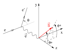
Figure 26: (Color online) Polar and azimuthal angles of the target spin.

direction, as shown in Fig. 26. We write them explicitly for a target with spin parallel to the beam direction as theory:he3elasym

$$\cos{\theta^{*}} = (E-E^{\prime}\cos{\theta})/|\vec{q}|$$ (57)

$$\phi^{*} = 0~{}.$$ (58)

The helicity-dependent part of the cross section can be written as

$$\Big{(}\frac{\mathrm{d}\sigma}{\mathrm{d}\Omega}\Big{)}^{h=+1}-\Big{(}\frac{\mathrm{d}\sigma}{\mathrm{d}\Omega}\Big{)}^{h=-1} = -\sigma_{Mott}\Big{(}V_{T^{\prime}}R_{T^{\prime}}(Q^{2})\cos\theta^{*}$$ (59)

$$+V_{TL^{\prime}}R_{TL^{\prime}}(Q^{2})\sin\theta^{*}\cos\phi^{*}\Big{)}~{},$$

with kinematic factors

$$V_{T^{\prime}} \equiv \tan{\frac{\theta}{2}}\sqrt{\frac{Q^{2}}{|\vec{q}|^{2}}+\tan^{2}{\frac{\theta}{2}}}$$ (60)

and

$$V_{TL^{\prime}} \equiv -\frac{Q^{2}}{\sqrt{2}|\vec{q}|^{2}}\tan{\frac{\theta}{2}}~{}.$$ (61)

$R_{T^{\prime}}$, $R_{TL^{\prime}}$ can be related to the ³He form factors $F_{c}$, $F_{m}$ as:

$$R_{T^{\prime}} = \frac{2\tau E^{\prime}}{E}(\mu_{{}^{3}\mathrm{He}}F_{m})^{2}$$ (62)

and

$$R_{TL^{\prime}} = -\frac{2\sqrt{2\tau(1+\tau)}E^{\prime}}{E}(ZF_{c})(\mu_{{}^{3}\mathrm{He}}F_{m})~{},$$ (63)

The elastic asymmetry, defined by

$$A^{el}_{\parallel}\equiv\frac{\big{(}\frac{\mathrm{d}\sigma}{\mathrm{d}\Omega\mathrm{d}E^{\prime}}\big{)}^{h=+1}-\big{(}\frac{\mathrm{d}\sigma}{\mathrm{d}\Omega\mathrm{d}E^{\prime}}\big{)}^{h=-1}}{\big{(}\frac{\mathrm{d}\sigma}{\mathrm{d}\Omega\mathrm{d}E^{\prime}}\big{)}^{h=+1}+\big{(}\frac{\mathrm{d}\sigma}{\mathrm{d}\Omega\mathrm{d}E^{\prime}}\big{)}^{h=-1}}~{},$$ (64)

can therefore be calculated from Eq. (53) and (59) as

$$A^{el}_{\parallel}=-(1-\tau)$$

$$\hskip 5.69046pt\cdot\frac{\big{(}{V_{T^{\prime}}R_{T^{\prime}}\cos\theta^{*}+V_{TL^{\prime}}R_{TL^{\prime}}\sin\theta^{*}\cos\phi^{*}}\big{)}}{\Bigl{\{}\frac{Q^{2}}{|\vec{q}|^{2}}F_{c}^{2}+\frac{\mu^{2}Q^{2}}{2M^{2}}\Big{(}\frac{1}{2}\frac{Q^{2}}{|\vec{q}|^{2}}-\tan^{2}{\frac{\theta}{2}}\Big{)}F_{m}^{2}\Bigr{\}}}~{}~{}~{}$$ (65)

ACKNOWLEDGMENTS

We would like to thank the personnel of Jefferson Lab for their efforts which resulted in the successful completion of the experiment. We thank S. J. Brodsky, L. Gamberg, N. Isgur, X. Ji, E. Leader, W. Melnitchouk, D. Stamenov, J. Soffer, M. Strikman, A. Thomas, M. Wakamatsu, H. Weigel and their collaborators for theoretical support and helpful discussions. This work was supported by the Department of Energy (DOE), the National Science Foundation, the Italian Istituto Nazionale di Fisica Nucleare, the French Institut National de Physique Nucléaire et de Physique des Particules, the French Commissariat à l’Énergie Atomique and the Jeffress Memorial Trust. The Southeastern Universities Research Association operates the Thomas Jefferson National Accelerator Facility for the DOE under contract DE-AC05-84ER40150.

References

- (1) J. Ashman et al., Phys. Lett. B 206, 364 (1988); J. Ashman et al., Nucl. Phys. B 328, 1 (1989).
- (2) M.J. Alguard et al., Phys. Rev. Lett. 41, 70 (1978); G. Baum et al., Phys. Rev. Lett. 51, 1135 (1983).
- (3) N.N. Bogoliubov, Ann. Inst. Henri Poincar 8, 163 (1968); F.E. Close, Nucl. Phys. B 80, 269 (1974); A. LeYaouanc et al., Phys. Rev. D 9, 2636 (1974); 15, 844 (1977); A. Chodos, R.L. Jaffe, K. Johnson, and C.B. Thorn, ibid. 10, 2599 (1974); M.J. Ruiz, ibid. 12, 2922 (1975); C. Hayne and N. Isgur, Phys. Rev. D 25, 1944 (1982). Z. Dziembowski, C.J. Martoff and P. Zyla, Phys. Rev. D 50, 5613 (1994). B.-Q. Ma, Phys. Lett. B 375, 320 (1996).
- (4) B.W. Filippone and X. Ji, Adv. Nucl. Phys. 26, 1 (2001). X. Ji, Phys. Rev. Lett. 78, 610 (1997).
- (5) R.P. Feynman, Phys. Rev. Lett. 23, 1415 (1969).
- (6) A.W. Thomas and W. Weise, The Structure of the Nucleon, p.78 and p.100, p.105-106, Wiley-Vch, Germany (2001).
- (7) K. Wilson, Phys. Rev. 179, 1499 (1969).
- (8) S. Wandzura and F. Wilczek, Phys. Lett. B, 72, 195 (1977).
- (9) R.L. Jaffe and X. Ji, Phys. Rev. D, 43, 724 (1991).
- (10) X. Ji and J. Osborne, Nucl. Phys. B 608, 235 (2001).
- (11) M. Göckeler et al., Phys. Rev. D 63, 074506 (2001).
- (12) R.L. Jaffe and X. Ji, Phys. Rev. D 43, 724 (1991); F.M. Steffens, H. Holtmann and A.W. Thomas, Phys. Lett. B 358, 139 (1995); X. Song, Phys. Rev. D 54, 1955 (1996).
- (13) E. Stein et al., Phys. Lett. B 343, 369 (1995); I. Balitsky, V. Braun and A. Kolesnichenko, ibid. 242, 245 (1990); 318, 648 (1993) (Erratum).
- (14) H. Weigel, L. Gamberg and H. Reinhardt, Nucl. Phys. A 680, 48c (2001); Phys. Rev. D 55, 6910 (1997); M. Wakamatsu, Phys. Lett. B 487, 118 (2000).
- (15) X. Zheng et al., Phys. Rev. Lett., 92, 012004 (2004).
- (16) G. Morpurgo, Physics 2, 95 (1965); R.H. Dalitz, in High Energy Physics; Lectures Delivered During the 1965 Session of the Summer School of Theoretical Physics, University of Grenoble, edited by C. De Witt and M. Jocab, Gordon and Breach, New York, 1965; and in Proceedings of the Oxford International Conference on Elementary Particles, Oxford, England, 1965;
- (17) F. Close, Nucl. Phys. B 80, 269 (1974); in An introduction to Quarks and Partons, p.197, Academic Press, New York (1979).
- (18) A. Bodek et al., Phys. Rev. Lett. 30, 1087 (1973); E.M. Riordan et al., ibid. 33, 561 (1974); J.S. Poucher et al., ibid. 32, 118 (1974).
- (19) A. Benvenuti et al., Phys. Lett. B 237, 599 (1990).
- (20) J.J. Aubert et al., Nucl. Phys. B 293, 740 (1987).
- (21) D. Allasia et al, Phys. Lett. B 249, 366 (1990); P. Amaudruz et al., Phys. Rev. Lett. 66, 2712 (1991); P. Amaudruz et al., Nucl. Phys. B 371, 3 (1992).
- (22) M.R. Adams et al, Phys. Rev. Lett. 75, 1466 (1995).
- (23) J. Ashman et al., Phys. Lett. B 206, 364 (1988); J. Ashman et al., Nucl. Phys. B 328, 1 (1989).
- (24) B. Adeva et al., Phys. Rev. D 60, 072004 (1999).
- (25) K. Abe et al., Phys. Rev. D 58, 112003 (1998).
- (26) F.E. Close, Phys. Lett. B 43, 422 (1973); R. Carlitz, ibid. 58, 345 (1975).
- (27) A. De Rujula, H. Georgi, S.L. Glashow, Phys. Rev. D 12, 147 (1975).
- (28) N. Isgur, Phys. Rev. D 59, 034013 (1999).
- (29) G.R. Farrar and D.R. Jackson, Phys. Rev. Lett. 35, 1416 (1975).
- (30) S.J. Brodsky, M. Burkardt and I. Schmidt, Nucl. Phys. B 441, 197 (1995).
- (31) E. Leader, A.V. Sidorov and D.B. Stamenov, Int. J. Mod. Phys. A 13, 5573 (1998).
- (32) D. Abbott et al., Phys. Rev. Lett. 84, 5053 (2000).
- (33) K. Wijesooriya et al., Phys. Rev. C 66, 034614 (2002).
- (34) M.K. Jones et al., Phys. Rev. Lett. 84, 1398 (2000).
- (35) O. Gayou et al., Phys. Rev. Lett. 88, 092301 (2002).
- (36) G.P. Lepage and S.J. Brodsky, Phys. Rev. D 22, 2157 (1981).
- (37) G.A. Miller and M.R. Frank, Phys. Rev. C 65, 065205 (2002);
- (38) R.V. Buniy, P. Jain and J.P. Ralston, AIP Conf. Proc. 549, 302 (2000).
- (39) A.V. Belitsky, X. Ji and Feng Yuan, Phys. Rev. Lett. 91, 092003 (2003).
- (40) X. Ji, J.-P. Ma and F. Yuan, Nucl. Phys. B 652, 383 (2003).
- (41) E. Leader, A.V. Sidorov and D.B. Stamenov, Eur. Phys. J. C 23, 479 (2002); E. Leader, D.B. Stamenov, priv. comm.
- (42) C. Bourrely, J. Soffer and F. Buccella, Eur. Phys. J. C 23, 487 (2002). C. Bourrely, J. Soffer, priv. comm.
- (43) H. Weigel, L. Gamberg and H. Reinhardt, Phys. Lett. B 399, 287 (1997); Phys. Rev. D 55, 6910 (1997); O. Schröder, H. Reinhardt and H. Weigel, Nucl. Phys. A 651, 174 (1999).
- (44) M. Wakamatsu, Phys. Rev. D 67, 034005 (2003); ibid. 67, 034006 (2003).
- (45) N.I. Kochelev, Phys. Rev. D 57, 5539 (1998).
- (46) E.D. Bloom and F.J. Gilman, Phys. Rev. Lett. 16, 1140 (1970); Phys. Rev. D 4, 2901 (1971);
- (47) F.E. Close and W. Melnitchouk, Phys. Rev. C 68, 035210 (2003); priv. comm.
- (48) C. Boros and A.W. Thomas, Phys. Rev. D 60, 074017 (1999); F.M. Steffens and A.W. Thomas, priv. comm.
- (49) D. Adams et al., Phys. Lett. B 357, 248 (1995).
- (50) K. Ackerstaff et al., Phys. Lett. B 404, 383 (1997).
- (51) P.L. Anthony et al., Phys. Rev. D 54, 6620 (1996).
- (52) K. Abe et al., Phys. Rev. Lett. 79, 26 (1997); Phys. Lett. B 405, 180 (1997).
- (53) P.L. Anthony et al., Phys. Lett. B 493, 19 (2000).
- (54) A. Airapetian et al., Phys. Lett. B 442, 484 (1998).
-
(55)
JLAB E99117, J.-P. Chen, Z.-E. Meziani, P. Souder et al.,
http://hallaweb.jlab.org/physics/experiments/he3/A1n/ - (56) A. Nogga, Ph. D. thesis, Ruhr-Universität Bochum, Bochum, Germany (2001), p.72.
- (57) J.L. Friar et al., Phys. Rev. C 42, 2310 (1990).
- (58) X. Zheng, Ph. D. thesis, M.I.T., Cambridge, Massachusetts (2002).
- (59) R. Prepost and T. Maruyama, Ann. Rev. of Nucl. and Part. Sci. 45, 41 (1995).
- (60) J. Alcorn et al., Nucl. Inst. Meth. A 522, 294 (2004).
- (61) J. Berthot and P. Vernin, Nucl. Phys. News 9, 12 (1990).
- (62) D. Marchand, Ph. D. thesis, Université Blaise Pascal, Clermont-Ferrand, France (1997).
- (63) O. Ravel, Ph. D. thesis, Université Blaise Pascal, Clermont-Ferrand, France (1997).
- (64) M. Baylac, Ph.!D. thesis, Universite Claude Bernard Lyon I, France (2000).
- (65) G.W. Miller IV, Ph. D. thesis, Princeton University, Princeton, New Jersey (2001).
- (66) K.G. Fissum et al., Nucl. Instrum. Meth. A 474, 108 (2001).
- (67) C. Grupen, Particle Detectors, p.193, Cambridge Univ., (1996).
- (68) W.A. Watson et al., Real-time Computer Applications in Nuclear, Particle and Plasma Physics, p.296-303, Vancouver, (1993).
-
(69)
E.A.J.M. Offerman, ESPACE User’s Guide,
http://www.hallaweb.jlab.org/espace/docs.html - (70) F.D. Colegrove, L.D. Shearer and G.K. Walters, Phys. Rev. 132, 2561 (1963).
- (71) W. Happer, Rev. Mod. Phys. 44, 169 (1972); S. Appelt et al., Phys. Rev. A 58, 1412 (1998).
- (72) T.E. Chupp et al., Phys. Rev. C 36, 2244 (1987).
-
(73)
JLab E94-010, G.D. Cates, J.P. Chen, Z.-E. Meziani et al.,
see http://www.jlab.org/e94010/ for technical notes; M. Amarian et al., Phys. Rev. Lett. 89, 242301 (2002); M. Amarian et al., ibid. 92, 022301 (2004). - (74) M.V. Romalis, Ph. D. thesis, Princeton University, Princeton, New Jersey (1998).
- (75) K. Kramer, Ph. D. thesis, College of William and Mary, Williamsburg, Virginia (2003).
- (76) M.V. Romalis and G.D. Cates, Phys. Rev. A 58, 3004 (1998).
- (77) A. Abragam, Principles of Nuclear Magnetism, Oxford Univ., (1961).
- (78) A. Deur, Ph. D. thesis, Université Blaise Pascal, Clermont-Ferrand, France (2000).
- (79) I. Akushevich et al., Comp. Phys. Comm. 104, 201 (1997).
- (80) L. Mo and Y.S. Tsai, Rev. Mod. Phys. 41, 205 (1969).
- (81) S. Stein et al., Phys. Rev. D 12, 1884 (1975); F.W. Brasse et al., Nucl. Phys. B 110, 413 (1976); P. Amaudruz et al., Phys. Lett. B 295, 159 (1992).
- (82) P. Amaudruz et al., Nucl. Phys. B 371, 3 (1992).
- (83) M. Arneodo et al., Phys. Lett. B 364, 107 (1995).
- (84) C. Keppel, Ph. D. thesis, American University, Washington DC (1994).
- (85) C. Keppel, Y. Liang, pri. comm.
- (86) L.W. Whitlow et al., Phys. Lett. B 250, 193 (1990).
- (87) K. Abe et al., Phys. Lett. B 452, 194 (1999).
- (88) A. Schaefer, Phys. Lett. B 208, 175 (1988).
- (89) M. Gluck, E. Reya, M. Stratmann and W. Vogelsang, Phys. Rev. D 53, 4775 (1996).
- (90) W. Melnitchouk and A. W. Thomas, Acta Phys. Polon. B 27, 1407 (1996); W. Melnitchouk, pri. comm.
- (91) Y.S. Tsai, in Proceedings of the International Conference on Nuclear Structure, p.221, Stanford Univ., 1964.
- (92) S.I. Bilenkaya, Y.M. Kazarinov and L.I. Lapidus, Pisma ZhETF, 61, 2225 (1971); Sov. Phys. JETP 34, 1192 (1972); Pisma ZhETF, 19, 613 (1974).
- (93) R. Arnold et al., Phys. Rev. Lett. 57, 174 (1986).
- (94) S. Galster et al., Nucl. Phys. B 32, 221 (1971).
- (95) I. Niculescu et al., Phys. Rev. Lett. 85, 1186 (2000).
- (96) MAID 2003, D. Drechsel, S.S. Kamalov and L. Tiator, Nucl. Phys. A 645, 145 (1999); http://www.kph.uni-mainz.de/MAID/maid2003/maid2003.html
- (97) F. Bissey et al., Phys. Rev. C 65, 064317 (2002).
- (98) C. Ciofi degli Atti et al., Phys. Rev. C 48, R968 (1993).
- (99) F. Bissey et al., Phys. Rev. C 64, 024004 (2001);
- (100) Y. Kolomensky, priv. comm.
- (101) K. Ackerstaff, et al, Phys. Lett. B 464, 123 (1999).
- (102) P.L. Anthony et al., Phys. Lett. B 553, 18 (2003).
- (103) N. Liyanage, JLAB Hall A Technical Note JLAB-TN-01-049 (2001), (unpublished).
- (104) H. Ibrahim, P. Ulmer and N. Liyanage, JLAB Hall A Technical Note JLAB-TN-02-032 (2002), (unpublished).
- (105) W. Melnitchouk, A. W. Thomas, Phys. Lett. B 377, 11 (1996).
- (106) A. Airapetian et al., Phys. Rev. Lett 92, 012005 (2004); M. Beckmann, D. Ryckbosch and E.C. Aschenauer, priv. comm.
- (107) J. Pumplin et al., J. High Energy Phys. 7, 012 (2002).
- (108) A.D. Martin, R.G. Roberts, W.J. Stirling and R.S. Thorne, Eur. Phys. J. C 23, 73 (2002).
- (109) Y. Goto et al., Phys. Rev. D 62, 034017 (2000).
- (110) J. Bluemlein and H. Boettcher, Nucl. Phys. B 636, 225 (2002).
- (111) M. Glueck, E. Reya, M. Stratmann and W. Vogelsang, Phys. Rev. D 63, 094005 (2001).
- (112) M. Anselmino, A. Efremov and E. Leader, Phys. Rept. 261, 1 (1995); Erratum-ibid. 281, 399 (1997).
- (113) J.D. Bjorken and E.A. Paschos, Phys. Rev. 185, 1975 (1969).
- (114) H.W. Kendall, Rev. Mod. Phys. 63, 597 (1991).
- (115) C.G. Callan, Jr. and D.J. Gross, Phys. Rev. Lett. 22, 156 (1969).
- (116) B. Foster, A.D. Martin and M.G. Vincter, Phys. Rev. D. 66, 010001 (2002).
- (117) Y. Dokshitzer, Sov. Phys. JETP 46, 1649 (1977); V.N. Gribov and L.N. Lipatov, Sov. Nucl. Phys. 15, 438 and 675 (1972); G. Altarelli, G. Parisi, Nucl. Phys. B 126, 298 (1977).
- (118) D. Drechsel, S.S. Kamalov and L. Tiator, Phys. Rev. D, 63, 114010 (2001).
- (119) J. Soffer, and O.V. Teryaev, Phys. Lett. B 490, 106 (2000).
- (120) P.S. Cooper et al., Phys. Rev. Lett. 34, 1589 (1975).
- (121) A. Amroun et al., Nucl. Phys. A 579, 596 (1994).
- (122) T.W. Donnelly and A.S. Raskin, Ann. Phys. (N.Y.) 169, 247 (1986).