Near threshold electroproduction of the $\omega$ meson at Q${\mathbf{{}^{2}}}\approx$ 0.5 GeV²

Abstract

Electroproduction of the $\omega$ meson was investigated in the ¹H$(e,e^{\prime}p)\omega$ reaction. The measurement was performed at a 4-momentum transfer $Q^{2}$ $\approx$ 0.5 GeV${}^{\textrm{2}}$. Angular distributions of the virtual photon-proton center-of-momentum cross sections have been extracted over the full angular range. These distributions exhibit a strong enhancement over $t$-channel parity exchange processes in the backward direction. According to a newly developed electroproduction model, this enhancement provides significant evidence of resonance formation in the $\gamma^{*}p\longrightarrow\omega p$ reaction channel.

I INTRODUCTION

There are only few measurements of the cross section for electroproduction of light vector mesons in the near threshold regime Joos et al. (1976, 1977). These experiments, carried out at DESY, despite suffering from very low statistics revealed that different mechanisms contribute to production of the $\rho^{0}$ and $\omega$ mesons in this region. The data for both the energy dependence and angular distribution of $\rho^{0}$ meson electroproduction were found to be consistent with a vector meson dominance (VMD) model described by t-channel particle exchange with natural or unnatural parity. This production mechanism is represented by the t-channel diagrams of Fig. 1. Diffractive scattering, interpreted as t-channel Pomeron exchange in the language of Regge theory, is the dominant process in the natural parity exchange mechanism above the traditional resonance region. Near the $\omega$ production threshold, because of the appreciable relative decay width $\Gamma_{\omega\rightarrow\pi^{0}\gamma}$ ($\sim\textrm{8}\%$), t-channel unnatural parity exchange, mediated by the exchange of the $\pi^{0}$ meson, can make significant, even dominant, contributions to $\omega$ electroproduction.

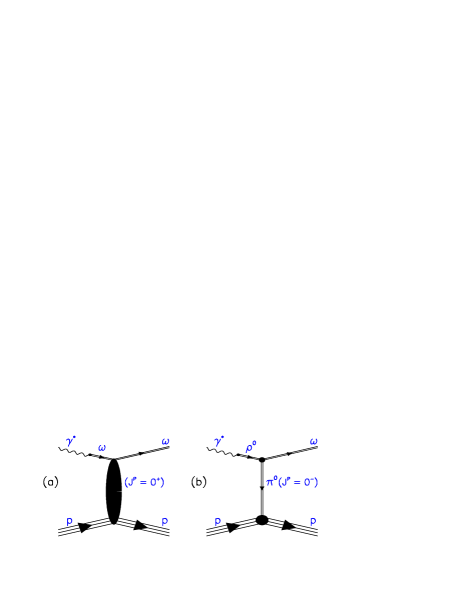
Figure 1: Vector meson dominance $t$-channel contributions: (a) diffractive scattering - natural parity exchange, (b) $\pi^{0}$ exchange - unnatural parity exchange.

A VMD-based model Fraas (1971), which includes both of these mechanisms fails, however, to reproduce the electroproduction data near threshold Joos et al. (1977). It was found that the strength of the total cross section at threshold is much larger than that predicted for the $t$-channel exchange contributions. This enhancement was associated with the non-peripheral component of the total cross section corresponding to large $t$ or, equivalently, backward scattering angles. Theoretical models based on $t$-channel exchange predict a strongly forward peaked angular distribution of the cross section that monotonically decreases with increasing angle. The results presented in this paper substantially differ from this prediction. Such discrepancies were suggested by other earlier measurements which, as in Ref. Joos et al. (1977), found disagreements in the energy dependence of the total cross section ABBHHM  Collaboration (1968); Klein (1996). More recent theoretical models address this by including $s$-channel and $u$-channel contributions to compensate for the additional strength at threshold.
The data for the present analysis were acquired in Hall C at the Thomas Jefferson National Accelerator Facility (Jefferson Lab) during an experiment designed to study electroproduction of strangeness via ${}^{1}{\textrm{H}}(e,e^{\prime}K^{+})\Lambda(\Sigma)$ e (91). Part of the background in the kaon electroproduction experiment were moderately inelastic $e^{\prime}p$ events rejected in the analysis by kaon particle identification. These $e^{\prime}p$ events, analyzed in the present work, provide the largest, to date, available data set on $\omega$ meson electroproduction.
This work reports on a measurement of the differential cross section for electroproduction of $\omega$ mesons observed in the ${}^{1}{\textrm{H}}(e,e^{\prime}p)\omega$ reaction near threshold at four-momentum transfer $Q^{2}\approx 0.5$ GeV². The detailed analysis can be found in Ref. Ambrozewicz (2001).

II EXPERIMENT

The experiment was conducted in Hall C at Jefferson Lab. The layout of the instrumentation is indicated in Fig. 2. Data were taken using 3.245 GeV electrons impinging on a 4.36-cm long target cell Dunne (1997); Meekins (1998). Liquid hydrogen circulating through the cell was cooled in a heat exchanger by 15 K gaseous helium and kept at a temperature of (19$\pm$0.2) K and a pressure of 24 psia.

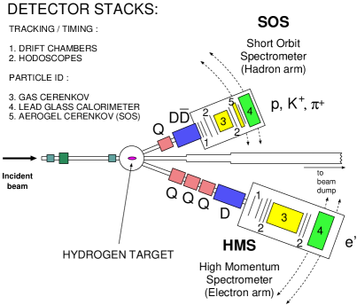
Figure 2: Top view of Hall C. Q and D denote quadrupole and dipole magnets respectively.

The experiment used the High Momentum Spectrometer (HMS) to detect scattered electrons. Its geometrical acceptance of $\sim 6.8$ msr was defined by an octagonal aperture in a 6.35-cm thick tungsten collimator. Before being detected, the electrons traversed the magnetic field of four superconducting magnets; three quadrupoles followed by a dipole. A pair of drift chambers at the focal plane of the spectrometer was used to determine the electron momentum while a threshold gas Čerenkov detector and Pb-glass calorimeter provided particle identification at both hardware (trigger) and software levels. Arrays of segmented scintillator hodoscopes were used to form the trigger and provide time-of-flight (ToF) measurements. All of the $\omega$ data were taken with an HMS spectrometer central angle of 17.20^∘ and a central momentum of 1.723 GeV. This choice defined the virtual photon flux centered at 17.67^∘ from the beam direction, and the four-momentum transfer $Q^{2}\approx$ 0.5 GeV${}^{\textrm{2}}$.

Table 1: Central values of the hadron arm momentum $p_{0}$, angular setting $\theta_{0}$, as well as the corresponding virtual photon proton separation $\theta_{\gamma p}$, and virtual photon $\omega$ meson CM angle $\theta^{*}$.

$p_{0}$ (GeV)	$\theta_{0}$ (deg)	$\theta_{\gamma p}$ (deg)	$\theta^{*}$ (deg)
1.077	17.67	0.00	180
	22.00	4.33	155
	26.50	8.78	135
	31.00	13.3	115
0.929	17.67	0.00	180
	22.00	4.33	130
	26.50	8.78	110
	31.00	13.3	95
	35.00	17.3	85
0.650	17.67	0.00	0
	22.00	4.33	15
	26.50	8.78	25

The Short Orbit Spectrometer (SOS) was set to detect positively charged particles ($\pi^{+}$, $K^{+}$ or $p$) and served as the hadron arm in the experiment. An octagonal aperture in a 6.35-cm thick tungsten collimator defined the SOS solid angle acceptance to be roughly 7.5 msr. Hadrons were detected after passing through the magnetic field of three resistive magnets; a quadrupole and two dipoles with opposite bending directions. A detector package similar to that of the HMS allowed for momentum determination (multi-wire drift chambers) and particle identification (segmented hodoscope arrays and Čerenkov detectors). Having fixed the electron arm position and momentum, the angular $\theta_{0}$ and momentum $p_{0}$ setting of the hadron arm was varied to access different scattering angles $\theta^{*}$ in the hadron ($\gamma^{*}p$) center-of-momentum (CM) system. These spectrometer settings, which corresponded to increasing virtual photon proton angular separation $\theta_{\gamma p}$ in the lab, allowed complete coverage for the $\omega$ scattering angles $\theta^{*}$ with respect to the virtual photon direction in the CM frame, particularly backward of 60^o. The data taken for the forward angles suffered from very low statistics. All the settings are presented in Table 1.

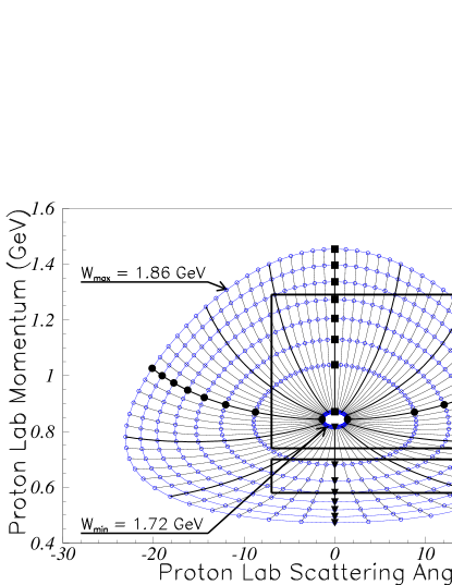
Figure 3: Total kinematic coverage. Straight lines define the acceptance of the experimental apparatus for all the kinematic settings.

Figure 3 shows the full kinematic coverage of the data set in conjunction with the available acceptance. The closed curves in this figure are contours of constant invariant mass $W$ and the radial lines are contours of constant scattering angle $\theta^{*}$ in the hadron CM frame. Open circles are at 20 MeV and 5 degree increments, respectively. The plot was generated for the $\omega$ mass, 0.782 GeV, and $Q^{2}=0.5$ GeV${}^{{\textrm{2}}}$. It is evident from this plot that a finite acceptance in proton lab momentum can produce cuts in which the range of accepted $W$ is a strong function of $\theta^{*}$. These correlations were accounted for in the extraction of the differential cross sections from the data.

III DATA ANALYSIS

Inelastic electron-proton final states were relatively easy to identify. Electrons were well separated from pions at the trigger level and final purification was achieved by using cuts on detector responses from the HMS gas Ĉerenkov detector and the Pb-glass calorimeter. Protons were selected using two types of scintillator timing information, time-of-flight (ToF) and coincidence time. In the SOS, the ToF was measured between two pairs of segmented hodoscope arrays separated by $1.76$ m. In addition, relative coincidence time was measured between the hadron and electron arm scintillator arrays. The top plots in Fig. 4 show typical distributions of ToF velocity, $\beta_{{\textrm{ToF}}}$, and coincidence time.

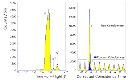
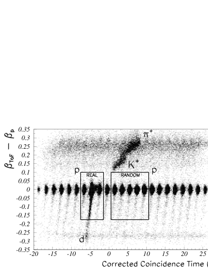
Figure 4: Top left: Velocity distribution from the time-of-flight measurement ($\beta_{{\textrm{ToF}}}$) for the real coincidence time cut shown in the bottom plot and described in the text. Top right: Distribution of the corrected coincidence time for protons. The estimated random coincidence contribution is overlayed on top of the coincident proton peak. Protons were selected using the ToF cut shown in the bottom plot. Bottom: Typical spectrum of the difference in the velocities as determined by the time-of-flight technique and proton momentum versus the corrected coincidence time.

The relatively large momentum acceptance, $\pm 20\%$ of the central setting (Table 1), resulted in a variation of velocity with momentum (manifested as an asymmetry in the proton $\beta_{{\textrm{ToF}}}$ distribution, see Fig. 4 top left). This, together with the associated pathlength variations, required corrections to the coincidence time to account for deviations from the central trajectory. The corrected coincidence time distribution (Fig. 4 top right) clearly shows the $2$ ns radio frequency (RF) microstructure of the electron beam. This structure was essential in the proton identification and accidental background removal. Real coincidence events, $e^{\prime}p$ pairs coming from the same interaction point, form a prominent peak at $-4.5$ ns. The remaining peaks are formed by random coincidences.
The final sample of protons was selected by requiring the corrected coincidence time to be within the three RF peaks centered on the true coincidence peak and by employing a cut, for improved selectivity, on the difference between ToF velocity $\beta_{{\textrm{ToF}}}$ and the velocity calculated using the measured proton momentum $\beta_{p}$. This combination of cuts allowed the retention of those protons that underwent interactions in the SOS detector hut. These events form a shoulder that extends from the proton coincident peak toward negative values of $\beta_{{\textrm{ToF}}}-\beta_{p}$ (Fig. 4 bottom).
Random coincidences, also present beneath the true coincidence peak (Fig. 4 top right), contributed a background in the final data sample (Fig. 7). These were averaged and removed by selecting a sample of random coincidences from five RF peaks (the selection procedure is shown in the bottom of Fig. 4). The random-subtracted distribution for any physics quantity was then obtained by subtracting the corresponding distribution for real and random samples, weighted by a 3:5 ratio to account for the differing numbers of peaks in the respective samples.

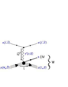
Figure 5: Fixed target ${\mathrm{{}^{1}H(e,e^{\prime}p)X}}$ scattering process. Here, as well as in the text below, the energy and three-momentum transfer $\nu$ and $\vec{q}$ are given by $\nu=E-E^{\prime}$ and $\vec{q}=\vec{k}-\vec{k}^{\prime}$.

The kinematics of the $\omega$ channel for a fixed target is diagrammatically shown in Fig 5. Kinematic quantities characterizing the process can be expressed employing the notation of Fig. 5:

$$Q^{2} = -[(E,\vec{k}\;)-(E^{\prime},\vec{k}^{\prime})]^{2}\stackrel{{\scriptstyle\;m_{e}\rightarrow 0\,}}{{\approx}}4EE^{\prime}\sin^{2}\left(\theta_{e^{\prime}}/2\right)\;,$$ (1)

$$W^{2} = [(M_{p},\vec{0}\;)+(\nu,\vec{q}\;)]^{2}=M_{p}^{2}+2M_{p}\nu-Q^{2}\;,$$ (2)

$$t\;\; = [(M_{p},\vec{0}\;)-(E_{p},\vec{p}\;)]^{2}=2M_{p}(M_{p}-E_{p})\;,$$ (3)

$$M^{2} = [(M_{p},\vec{0}\;)+(E,\vec{k}\;)-(E^{\prime},\vec{k}^{\prime})-(E_{p},\vec{p}\;)]^{2}=$$ (4)

$$= W^{2}+M_{p}^{2}-2E_{p}(M_{p}+\nu)+2|{\vec{q}}\,||{\vec{p}}\,|\cos\theta_{\gamma p}\;,$$

where $\theta_{e^{\prime}}$ is the laboratory electron scattering angle and $\theta_{\gamma p}$ is the proton scattering angle with respect to the virtual photon direction. $Q^{2}$ is square of the four-momentum transfer to the target, $W$ is the invariant mass of the virtual photon-proton system, $t$ is the squared four-momentum transfer to the proton, and $M$ is the mass of the system of undetected particles.

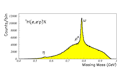
Figure 6: Light vector meson electroproduction. The histogram shows events for all accepted momenta for one setting. Note the presence of the pseudoscalar $\eta$ meson signal.

Reconstruction of the missing mass, performed according to Eqn. (4), reveals a spectrum with a strong $\omega$ meson signal atop a complicated background (Fig. 6). The data were corrected for trigger inefficiency ($<\!{\mathrm{1}}\%$), track reconstruction inefficiencies ($\sim$10$\%$), particle ID inefficiencies ($\sim$2$\%$), and computer and electronic dead times ($\sim$5$\%$). In the CM system, the virtual photon cross section for $\omega$ production ${d\sigma_{v}}/{d\Omega^{*}}$ is given in terms of the conventional two-particle coincidence cross section

$$\frac{d\sigma}{dp_{e^{\prime}}d\Omega_{e^{\prime}}d\Omega^{*}}=\Gamma_{T}\;\frac{d\sigma_{v}}{d\Omega^{*}}\;,$$ (5)

where $\Gamma_{T}$ is the virtual photon flux. The virtual photon cross section can be decomposed into transverse ($\sigma_{T}$), longitudinal ($\sigma_{L}$), and interference terms ($\sigma_{TT}$, $\sigma_{LT}$), such that

$$\frac{d\sigma_{v}}{d\Omega^{*}}=\sigma_{U}+\varepsilon\,\cos 2\phi^{*}\,\sigma_{TT}+\sqrt{\frac{\varepsilon(\varepsilon+1)}{2}}\cos\phi^{*}\,\sigma_{LT}\;,$$ (6)

where $\sigma_{U}=\sigma_{T}+\varepsilon\,\sigma_{L}$, $\varepsilon$ is the virtual photon polarization parameter, and $\phi^{*}$ is the relative angle between the electron scattering plane and hadron production plane.

The biggest challenge in cross section extraction was the separation of the data into the physics backgrounds and $\omega$ meson production (Fig. 7). This was accomplished by using a Monte Carlo program to simulate both processes, the dominant background as well as $\omega$ production. The background was modeled as a combination of two processes, electroproduction of the neutral $\rho$ meson and multi-pion production.

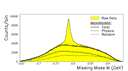
Figure 7: Missing mass distribution for ¹H$(e,e^{\prime}p)X$ showing the decomposition into a peak for $\omega$ and the background.

Production of the $\rho$ was assumed to be purely diffractive Fraas and Schildknecht (1969),

$$\frac{d\sigma}{d\Omega^{*}dM}=\left(\frac{M_{\rho}}{M}\right)^{n}\;B_{\rho}(M)\;\;De^{bt^{\prime}}\;,$$ (7)

where $t^{\prime}=t-t_{{\textrm{min}}}$, with $t_{{\textrm{min}}}$ being the momentum transfer when the scattering occurs along the virtual photon direction. In the above expression, coefficients $D$ and $b$ are $Q^{2}$ and $W$ dependent to account for their variation near threshold and $D$, at $Q^{2}=0$, corresponds to the photoproduction cross section. The skewness of the $\rho$ meson shape, apparent from other experiments, was accounted for by using the Ross-Stodolsky parameterization Ross and Stodolsky (1966) (in Eqn. (7) first factor on the right-hand side) with the exponent $n=5.2$ coming from a fit to the DESY data Joos et al. (1976). For both the background and the $\omega$ meson, the mass distributions were generated according to a fixed width relativistic Breit-Wigner distribution

$$B_{v}(M)=\frac{M_{v}^{2}\Gamma_{v}^{2}}{(M^{2}-M_{v}^{2})^{2}+M_{v}^{2}\Gamma_{v}^{2}}\;,$$ (8)

where $v$ is $\rho$ or $\omega$ with $M_{\omega}=781.94$ MeV, $\Gamma_{\omega}=8.43$ MeV, $M_{\rho}=768.1$ MeV, and $\Gamma_{\rho}=150.7$ MeV Caso et al. (1998).

The multi-pion processes were collectively modeled as a Lorentz invariant electroproduction phase space for two-body production of a fictitious particle with arbitrary mass M. This term is meant to account for all physically allowed reactions ($W$ is well above the $\pi\pi$ threshold) that result in more than three particles (including the electron and proton) in the final state. The flatly distributed low yield of events (approximately $2\%$ at most settings) coming from the aluminum walls of the liquid hydrogen target were also treated as a part of the phase space background. The phase space was simulated by

$$\frac{d\sigma}{d\Omega^{*}dM}=\frac{1}{32\pi^{2}}\left(\frac{p^{*}}{q^{*}}\right)\frac{M}{W^{2}}\;,$$ (9)

where $q^{*}$ and $p^{*}$ are the initial and final momenta in the CM frame, respectively.

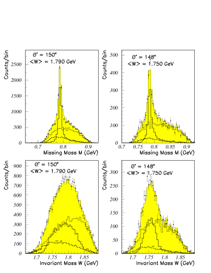
Figure 8: Missing mass $M$ and invariant mass $W$ distributions broken down into individual contributions for two different momentum settings but the same angular settings. Solid circles with error bars are the data. The shaded histogram is the full Monte Carlo fit. The dotted line histogram corresponds to the resulting phase space yield, the solid line histogram to the $\omega$ yield, and the dashed line histogram to the $\rho^{0}$ yield.

The production of the $\omega$ meson was simulated with a cross section assumed to be $t$-channel unnatural parity exchange

$$\frac{d\sigma}{d\Omega^{*}dM}=B_{\omega}(M)\;(\sigma_{T}^{\pi}+\varepsilon\,\sigma_{L}^{\pi})\,,$$ (10)

with $\sigma_{T}^{\pi}$, $\sigma_{L}^{\pi}$ being the transverse and longitudinal parts of the corresponding cross section Fraas (1971). Within this model, the longitudinal contribution $\sigma_{L}^{\pi}$ is insignificant because it is an order of magnitude smaller than $\sigma_{T}^{\pi}$ for the kinematic regime of the experiment. Natural parity exchange was neglected because it is also roughly one order of magnitude smaller than $\sigma_{T}^{\pi}$ within this regime. Similarly neglected were the nearly vanishing contributions from the interference terms $\sigma_{TT}$ and $\sigma_{LT}$. This amounts to modeling the total cross section using only the largest contribution.

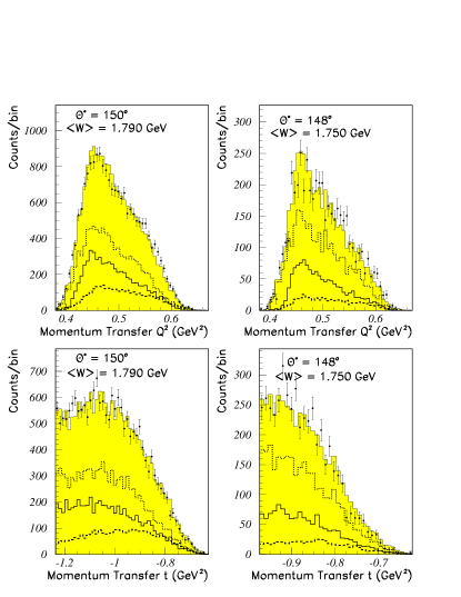
Figure 9: Distributions of four-momentum transfers $Q^{2}$ and $t$ for the same settings as described in the caption of Fig. 8. The cut-off at low values of $-t$ reflects the proton momentum cut applied in the analysis since the proton energy is directly proportional to $t$ in the fixed target regime (see Eqn. 3).

The Monte Carlo program simulated finite target effects (multiple scattering and ionization energy losses), acceptance corrections, and radiative proccesses. The radiative corrections were modeled after the approximations from Ref. Ent et al. (2001). They were accounted for by altering the incident and scattered electron kinematics and applying loop and vertex corrections which modify the cross section, but do not modify the missing mass distribution. Having simulated all the processes for each kinematic setting, the data and Monte Carlo events were binned in CM scattering angle $\theta^{*}$. Finally, a binned maximum likelihood fit was performed simultaneously in missing mass, $W$, $Q^{2}$, $t$, and $\theta^{*}$. The approach incorporated in the fit was developed by R. Barlow Barlow (1993). The likelihood function accounted for fluctuations in the data and Monte Carlo distributions due to finite statistics. Its maximization allowed the search for the overall strengths, $p_{i}$, of each process modeled, so that the resulting yields for each bin satisfy the relation

$$Y_{\mathrm{DATA}}=Y_{\mathrm{MC}}=p_{1}\,Y_{\omega}+p_{2}\,Y_{\rho}+p_{3}\,Y_{\mathrm{phsp}}\;.$$ (11)

Results of the fitting process for the high momentum setting of the hadron arm, $p_{0}^{{\textrm{SOS}}}=1.077$ GeV, and the intermediate momentum setting, $p_{0}^{{\textrm{SOS}}}=0.929$ GeV, for the same angular setting of $\theta_{\gamma{\textrm{p}}}=4.33^{o}$, are shown in Fig. 8 and Fig. 9. Figures 10 and 11 show the result of summation of the fits for all $\theta^{*}$ bins within these two hadron arm settings, respectively, thus reflecting the goodness of the fit. Performing the fit allowed separation of the raw data into the Monte Carlo determined background, consisting of the $\rho$ meson and phase-space contributions, and the $\omega$ meson signal, thus obtaining the data yields (Fig. 12).

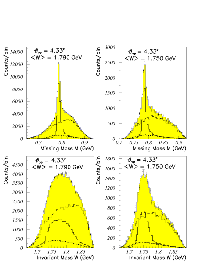
Figure 10: Fits for two different momentum settings summed over $\theta^{*}$ bins for missing mass (top) and invariant mass (bottom). Fig. 8 contains the legend explanation.

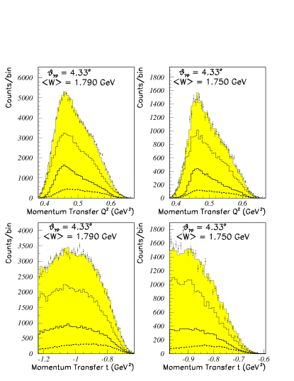
Figure 11: Fits for two different momentum settings summed over $\theta^{*}$ bins for four-momentum transfer $t$ (top) and four-momentum transfer $Q^{2}$ (bottom). Fig. 8 contains the legend explanation.

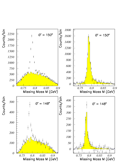
Figure 12: The results of signal-background separation, or, equivalently, $\omega$ yield extraction, for two different momentum settings of the hadron arm but the same, $\theta_{\gamma{\textrm{p}}}=4.33^{o}$, angular setting, Top: central momentum $p_{{\textrm{0}}}=1.077$ GeV. Bottom: central momentum $p_{{\textrm{0}}}=0.929$ GeV.

Subsequently, the differential virtual photon cross section was computed by scaling the model cross section by the data yield $Y^{\omega}_{DATA}$ ($\approx p_{1}\,Y_{\omega}$), normalized to the simulated yield

$$\frac{d\sigma_{v}}{d\Omega^{*}}=\frac{Y^{\omega}_{DATA}}{Y^{\omega}_{MC}}\;\left(\frac{d\sigma}{d\Omega^{*}}\right)_{MC}\;.$$ (12)

The Monte Carlo yield $Y^{\omega}_{MC}$ was evaluated by integrating the model cross section, $d\sigma$/$d\Omega^{*}dM$ over the entire acceptance of the apparatus and binning the result in the CM scattering angle. For any $\theta^{*}_{i}$ bin, this process can be expressed as

$$Y^{\omega}_{MC}=\int_{{\mathcal{A}}(\theta^{*}_{i})}\Gamma_{T}\,{\mathcal{R}}\,\frac{d\sigma}{d\Omega^{*}dM}\,dQ^{2}dWd\phi_{e^{\prime}}d\Omega^{*}dM\;,$$ (13)

where ${\mathcal{R}}$ represents the multiplicative part of the radiative corrections and ${\mathcal{A}}(\theta^{*}_{i})$ is the acceptance for the given $\theta^{*}_{i}$ bin. In the above expression, mass was integrated over the $\omega$ line shape (Eqn. 8). The cross section was extracted at $Q^{2}\approx 0.5$ GeV${}^{\textrm{2}}$ for 74 bins in $\theta^{{\textrm{*}}}$, mostly for backward directions in the $\gamma^{*}p$ CM system. Here, the Hand Hand (1963) convention was adopted in evaluating the virtual photon flux $\Gamma_{T}$. Identifying the $\omega$ meson production using only the $e^{\prime}p$ final states introduced a statistical error of less than $25\%$. Systematic uncertainties associated with the background subtraction are less than $12\%$. Fixed electron kinematics and limited out-of-plane acceptance reduced the range of accepted $\phi^{*}$ angles to $\pm 30^{\textrm{o}}$ about $0^{\textrm{o}}$ for the outermost angular setting ($\theta_{\gamma{\textrm{p}}}=17.3^{o}$). This $\phi$ cut was also applied to the data of all other settings.

IV RESULTS

With the use of the procedures described above, angular distributions of the differential cross sections for electroproduction of the $\omega$ meson were extracted for two different average values of the invariant mass $W$. The data were divided into two sets according to the average $W$ which, for each data point, was determined using the results of the fit. These two sets form the angular distributions that correspond to mean invariant masses $\langle W\rangle$ of 1.750 GeV and 1.790 GeV. The results are presented in Tables 2 and 3.

Table 2: Differential cross sections for the lower average $W$ (${\langle W\rangle}=1.75$ GeV). The bin width is 5⁰, centered on the quoted value, except for the first bin whose width is 10⁰. The cross sections were extracted for $|\phi^{*}|<30^{o}$.

$\theta^{*}$	$d\sigma/d\Omega^{*}$	Uncertainty		${{{\langle W\rangle}}}$	${{{\langle Q^{2}\rangle}}}$
(deg)	($\mu b/sr$)	Stat.	Syst.	(GeV)	$(GeV^{2})$
45	0.257	0.057	0.015	1.753	0.501
75	0.116	0.026	0.011	1.745	0.512
80	0.170	0.026	0.006	1.747	0.511
85	0.112	0.024	0.006	1.747	0.510
90	0.131	0.024	0.006	1.747	0.510
95	0.163	0.024	0.008	1.749	0.510
100	0.176	0.023	0.010	1.752	0.509
101	0.170	0.028	0.012	1.752	0.509
105	0.260	0.023	0.012	1.755	0.505
106	0.267	0.028	0.012	1.756	0.508
110	0.292	0.024	0.012	1.758	0.504
111	0.311	0.025	0.013	1.761	0.505
115	0.440	0.026	0.014	1.763	0.501
120	0.466	0.025	0.013	1.766	0.499
125	0.425	0.025	0.013	1.766	0.498
130	0.399	0.026	0.012	1.762	0.498
135	0.412	0.031	0.012	1.759	0.500
138	0.400	0.031	0.012	1.749	0.497
140	0.458	0.044	0.012	1.755	0.501
143	0.466	0.033	0.012	1.751	0.498
148	0.367	0.028	0.010	1.751	0.497
153	0.352	0.030	0.010	1.750	0.501
158	0.308	0.031	0.010	1.748	0.501
163	0.353	0.039	0.009	1.747	0.501
168	0.288	0.040	0.010	1.745	0.504
173	0.199	0.050	0.012	1.742	0.510

Table 3: Differential cross sections for the higher average $W$ (${\langle W\rangle}=1.790$ GeV). The bin width is 5⁰, centered on the quoted value, except for the first two bins whose width is 10⁰. The cross sections were extracted for $|\phi^{*}|<30^{o}$.

$\theta^{*}$	$d\sigma/d\Omega^{*}$	Uncertainty		${\langle W\rangle}$	${\langle Q^{2}\rangle}$
(deg)	($\mu b/sr$)	Stat.	Syst.	(GeV)	$(GeV^{2})$
25	0.501	0.058	0.015	1.778	0.505
35	0.360	0.053	0.015	1.765	0.502
62	0.229	0.034	0.015	1.808	0.493
67	0.263	0.030	0.014	1.808	0.489
72	0.186	0.027	0.014	1.811	0.488
73	0.171	0.033	0.014	1.771	0.504
77	0.193	0.025	0.014	1.814	0.484
78	0.168	0.032	0.014	1.773	0.503
82	0.141	0.023	0.013	1.819	0.479
83	0.175	0.030	0.013	1.775	0.502
84	0.173	0.030	0.012	1.780	0.512
88	0.225	0.029	0.012	1.779	0.500
87	0.226	0.024	0.012	1.821	0.477
89	0.256	0.024	0.012	1.782	0.502
92	0.251	0.027	0.012	1.825	0.475
93	0.249	0.028	0.012	1.784	0.496
94	0.237	0.020	0.012	1.789	0.498
97	0.282	0.031	0.012	1.827	0.473
98	0.329	0.027	0.012	1.791	0.493
99	0.321	0.019	0.012	1.800	0.491
102	0.309	0.047	0.012	1.827	0.470
103	0.395	0.028	0.011	1.798	0.489
104	0.352	0.018	0.012	1.808	0.485
108	0.365	0.030	0.012	1.796	0.488
109	0.391	0.020	0.011	1.811	0.484
113	0.318	0.037	0.012	1.791	0.488
114	0.450	0.023	0.011	1.814	0.481
116	0.396	0.025	0.011	1.772	0.500
119	0.515	0.029	0.011	1.816	0.481
121	0.486	0.024	0.010	1.785	0.493
124	0.524	0.044	0.010	1.816	0.482
126	0.503	0.023	0.010	1.795	0.488
131	0.506	0.024	0.010	1.796	0.488
136	0.518	0.027	0.010	1.792	0.490
140	0.530	0.024	0.010	1.772	0.489
141	0.495	0.031	0.010	1.788	0.492
145	0.538	0.020	0.010	1.781	0.488
146	0.536	0.046	0.010	1.779	0.501
150	0.492	0.019	0.010	1.783	0.489
151	0.471	0.102	0.014	1.765	0.516
155	0.431	0.019	0.010	1.780	0.492
160	0.425	0.021	0.010	1.777	0.494
165	0.439	0.026	0.010	1.773	0.498
166	0.652	0.093	0.014	1.785	0.470
170	0.442	0.036	0.011	1.764	0.504
171	0.419	0.059	0.012	1.780	0.482
175	0.485	0.070	0.012	1.755	0.513
176	0.392	0.077	0.014	1.778	0.489

These two sets of the data, however, do not constitute two independent angular distributions. There are large overlaps in the $W$ ranges for both distributions that can readily be seen in the bottom of Figs. 8 and 10. Therefore, the cross sections of both angular distributions were scaled to a reference $W$ of 1.785 GeV. This was done by rescaling their corresponding kinematic parts, i.e. phase space factors normalized to the incoming particle flux. Due to a significant variation with mass, the scaling factor was determined on an event-by-event basis and then averaged. The scaling can quantitatively be described by

$$\left(\frac{d\sigma}{d\Omega^{*}}\right)_{{\textrm{scaled}}}=\frac{\Gamma(W_{\textrm{ref}})}{\Gamma(W)}\;\frac{d\sigma}{d\Omega^{*}}\;,$$ (14)

where $\Gamma(W)=p^{*}(W)/q^{*}(W)W^{2}$ is a normalized phase space factor (compare with Eqn. (9)) and $p^{*}$ and $q^{*}$ are, respectively, the 3-momenta in the CM frame of the $\omega$ and the virtual photon which, for fixed $W$, are determined only by the masses of the interacting particles. The result of this procedure is shown in Fig. 13. Correcting for the phase space, opening up above the threshold, removes practically all of the observed $W$ dependence. It also shows that the shape of the distribution is not trivially induced by $W$ variations of the phase space factors.
The enhancement of the backward-angle cross section over $t$-channel unnatural parity exchange (Fraas model, dashed line) is evident. This was suggested by the earlier electroproduction Joos et al. (1977) and photoproduction ABBHHM  Collaboration (1968); Klein (1996) data. Such a departure from the smooth fall-off of the $t$-channel processes, either in the angular distribution or $t$-dependence, has been attributed, theoretically, to $s$- and $u$-channel resonance contributions. Even though the energy dependence may not be sensitive to the details of the model, since it is integrated over full angular range, the inclusion of resonance formation was also necessary to reproduce the near threshold strength of the photoproduction cross section (see Zhao (2000, 2001)).

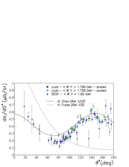
Figure 13: The angular distributions for different average $W$ and for $|\phi^{*}|<30^{o}$. Error bars are statistical. The DESY data correspond to the four-momentum transfer $Q^{\textrm{2}}=0.77$ GeV${}^{\textrm{2}}$, $W=1.82$ GeV and full $\phi^{*}$ range. The Fraas model shown here was used in the cross section extraction. Both distributions were scaled to $W=1.785$ GeV. The scaling procedure is described in the text.

Recent examples of such calculations Zhao (2000, 2001); Zhao et al. (1998a); Oh et al. (2000, 2001); Zhao et al. (1998b) mainly address SAPHIR data Klein (1996). Some of these works Oh et al. (2000, 2001) showed that the dominant contributions could come from the missing resonances, $N_{3/2}^{+}(1910)$, and the $N_{3/2}^{-}(1960)$ (the latter is labeled $D_{13}(2080)$ by the Particle Data Group). Other calculations, however, differ in predicting which nucleonic excitations could contribute in the $s$-channel. It was found that the contribution from two resonances, $P_{\textrm{1}3}$(1720) and $F_{\textrm{1}5}$(1680), dominated and their inclusion was necessary to reproduce the available photoproduction data near threshold Zhao (2000, 2001); Zhao et al. (1998a, b).
From the point of view of the present work, the most interesting result of these theoretical models is that the nucleon resonances are the favored mechanism for producing backward-angle enhancements in the differential cross section. The solid line in Fig. 13 shows the comparison of the data with an unpublished, as of this writing, electroproduction calculation Zhao (2003) complementary to the photoproduction model Zhao (2001). In this model, the diffractive nature of $\omega$ production is described by Pomeron exchange based on Regge phenomenology and SU(3) flavor symmetry. This contribution dominates the cross section above the resonance region. Neutral $\pi$ exchange in the $t$-channel is included to account for the peaking of the cross section in the forward direction, especially near threshold. Resonance formation processes in the $s$- and $u$-channel that dominate intermediate and backward scattering angles, where the other contributions are small, were modeled in an $SU(6)\times O(3)$ quark model symmetry limit. All contributions, summed coherently, give a strongly $\phi^{*}$-dependent cross section (Eqn. (6)). To correctly compare this theoretical calculation with the data, the model was integrated over a range of the azimuthal angle $\phi^{*}$ corresponding to the cut used in the data analysis. The model was also averaged over the appropriate $W$ and $Q^{\textrm{2}}$ ranges.

V CONCLUSIONS

Cross sections for the $\omega$ meson electroproduction were obtained from the ¹H$(e,e^{\prime}p)\omega$ reaction at $E_{e}=3.245$ GeV. The angular distribution of the differential cross section in the threshold regime has unprecedented granularity and much smaller statistical uncertainties than in previous work. The angular distribution exhibits a substantial backward-angle enhancement of the cross section over the pure $t$-channel expectation, similar to that found in the DESY Joos et al. (1977), photoproduction ABBHHM  Collaboration (1968), and SAPHIR data Klein (1996).

In comparing the result of this work to the Zhao model Zhao (2003), the similarity of the angular distributions is evident. In the view of these results, this analysis provides significant evidence for resonance formation, possibly $s$-channel, in the $\gamma^{\star}p\longrightarrow\omega p$ reaction. It is worth noting that, although elastic $\pi N$ scattering constitutes the main source of information on the nucleon excitation spectrum, it alone cannot distinguish among existing theoretical models Isgur and Koniuk (1980), many of which predict a much richer baryonic, hence nucleonic, spectrum than currently observed Isgur and Karl (1977, 1978a, 1978b, 1979); Capstick and Isgur (1986); Capstick and Roberts (1994); Capps (1974); Cutkosky and Hendrick (1977); Forsythe and Cutkosky (1983). If they exist, these states are either being masked by neighboring resonances with stronger couplings or they are altogether decoupled from the $\pi N$ channel. There are decay modes, other than $\pi N$, however, that have sizeable resonance coupling constants Capstick and Roberts (1994); Capstick (1992). A calculation, based on the symmetric quark model Capstick and Roberts (2000), indeed predicts that vector meson decay channels, $N\rho$ and $N\omega$, have appreciable resonance couplings. Electroproduction of $\omega$ mesons, enhanced by its isospin selectivity, may therefore provide additional evidence in the search for resonances unobserved in $\pi N$ scattering.

References

- Joos et al. (1976) P. Joos et al., Nucl. Phys. B113, 53 (1976).
- Joos et al. (1977) P. Joos et al., Nucl. Phys. B122, 365 (1977).
- Fraas (1971) H. Fraas, Nuclear Physics B36, 191 (1971).
- ABBHHM Collaboration (1968) ABBHHM Collaboration, Phys. Rev. 175, 1669 (1968).
- Klein (1996) F. Klein, Ph.D. thesis, Bonn University (1996).
- e (91) Jefferson Laboratory experiment E91-016 (Ben Zeidman spokesperson).
- Ambrozewicz (2001) P. Ambrozewicz, Ph.D. thesis, Temple University (2001).
- Dunne (1997) J. Dunne, Cryo and dummy target information (1997), JLab Hall C Internal Report (unpublished).
- Meekins (1998) D. Meekins, Ph.D. thesis, College of William & Mary (1998).
- Fraas and Schildknecht (1969) H. Fraas and D. Schildknecht, Nuclear Physics B14, 543 (1969).
- Ross and Stodolsky (1966) M. Ross and L. Stodolsky, Phys. Rev. 149, 1172 (1966).
- Caso et al. (1998) C. Caso et al., Eur. Phys. J. C3 (1998).
- Ent et al. (2001) R. Ent et al., Phys. Rev. 64, 054610 (2001).
- Barlow (1993) R. Barlow, Comp. Phys. Commun. 77, 219 (1993).
- Hand (1963) L. Hand, Phys. Rev. 129, 1834 (1963).
- Zhao (2000) Q. Zhao, Nucl. Phys. A675, 217 (2000).
- Zhao (2001) Q. Zhao, Phys. Rev. C 63, 025203 (2001).
- Zhao et al. (1998a) Q. Zhao, Z. Li, and C. Bennhold, Phys. Lett. B436, 42 (1998a).
- Zhao et al. (1998b) Q. Zhao, Z. Li, and C. Bennhold, Phys. Rev. C58, 2393 (1998b).
- Oh et al. (2000) Y. Oh, A. Titov, and T.-S. Lee (2000), arXiv:nucl-th/0004055 (preprint).
- Oh et al. (2001) Y. Oh, A. Titov, and T.-S. Lee, Phys. Rev. C 63, 025203 (2001).
- Zhao (2003) Q. Zhao, Private communication (2003).
- Isgur and Koniuk (1980) N. Isgur and R. Koniuk, Phys. Rev. D21, 1868 (1980).
- Capps (1974) R. Capps, Phys. Rev. Lett. 33, 1637 (1974).
- Capstick and Isgur (1986) S. Capstick and N. Isgur, Phys. Rev. D34, 2809 (1986).
- Capstick and Roberts (1994) S. Capstick and W. Roberts, Phys. Rev. D49, 4570 (1994).
- Cutkosky and Hendrick (1977) R. Cutkosky and R. Hendrick, Phys. Rev. D 16, 2902 (1977).
- Forsythe and Cutkosky (1983) C. Forsythe and R. Cutkosky, Z. Phys. C 18, 219 (1983).
- Isgur and Karl (1977) N. Isgur and G. Karl, Phys. Lett. 72B, 109 (1977).
- Isgur and Karl (1978a) N. Isgur and G. Karl, Phys. Lett. 74B, 353 (1978a).
- Isgur and Karl (1978b) N. Isgur and G. Karl, Phys. Rev. D18, 4187 (1978b).
- Isgur and Karl (1979) N. Isgur and G. Karl, Phys. Rev. D19, 2653 (1979).
- Capstick (1992) S. Capstick, Phys. Rev. D46, 2864 (1992).
- Capstick and Roberts (2000) S. Capstick and W. Roberts, Prog. Part. Nucl. Phys. 45, S241 (2000).