Measurements of electron-proton elastic cross sections for 0.4 $<$ $Q^{2}$ $<$ 5.5 $({\rm GeV}/c)^{2}$

Abstract

We report on precision measurements of the elastic cross section for electron-proton scattering performed in Hall C at Jefferson Lab. The measurements were made at 28 distinct kinematic settings covering a range in momentum transfer of $0.4<Q^{2}$ $<$ 5.5 $({\rm GeV}/c)^{2}$. These measurements represent a significant contribution to the world’s cross section data set in the $Q^{2}$ range where a large discrepancy currently exists between the ratio of electric to magnetic proton form factors extracted from previous cross section measurements and that recently measured via polarization transfer in Hall A at Jefferson Lab. This data set shows good agreement with previous cross section measurements, indicating that if a here-to-fore unknown systematic error does exist in the cross section measurements then it is intrinsic to all such measurements.

I Introduction

Recently, there has been much renewed interest in the proton electromagnetic form factors in the region of four-momentum transfer, $Q^{2}$ $>$ 1 $({\rm GeV}/c)^{2}$. This is due primarily to recent measurements from Hall A at Jefferson Lab jones ; gayou1 on the ratio of the Sachs electric to magnetic form factors via the polarization transfer technique pol1 ; pol2 . These data are in stark disagreement with previous extractions of these form factors litt ; price ; walker ; andiv from cross section measurements utilizing the Rosenbluth separation technique rosen .

There have been recent efforts brash ; arrington ; arrington2 to extract the individual form factors by combining the cross section and polarization transfer results. However, it is clear that the data sets from these two techniques are systematically inconsistent arrington and, as such, the method that one chooses for combining the data sets is not well defined. It is critical, then, that the source of the discrepancy be identified, if there is to be any chance of pinning down the $Q^{2}$ dependence of the individual form factors arrington2 .

In this paper we will present results from 28 new precision measurements of the ep elastic cross section in the range 0.4 $<$ $Q^{2}$ $<$ 5.5 $({\rm GeV}/c)^{2}$ performed in Hall C at Jefferson Lab. Although the kinematics are such that only limited Rosenbluth separations of the form factors can be performed, this data represents a significant contribution to the world’s cross section data set, and as such, can help provide new constraints on global fits from which the form factors can be extracted.

The high precision and large kinematic coverage of the new Jefferson Lab data can help provide crucial information as to whether there exists an experimental systematic error in the world’s cross section data set, which is dominated by the data from SLAC in the $Q^{2}$ range where the discrepancy with the polarization transfer data exists.

II ep Elastic Scattering

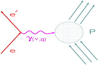
Figure 1: (Color online) Single photon exchange diagram for electron proton elastic scattering.

The elastic scattering of an electron from a proton target can be represented in the first order Born approximation by the exchange of a single virtual photon between the leptonic and hadronic electromagnetic currents. This exchange is represented by the diagram in Fig. 1 and is often referred to as the one photon exchange approximation (OPEA), with 4-momentum transfer

$$q_{\mu}=k^{\prime}_{\mu}-k_{\mu},$$ (1)

where $k_{\mu}$ ($k^{\prime}_{\mu}$) is the four-momentum of the electron before (after) scattering. For space-like photons ($q^{2}=q_{\mu}q^{\mu}$ $<$ 0) it is customary to define the absolute value of the square of the four-momentum transfer

$$Q^{2}\equiv-q^{2}\approx 4EE^{\prime}\sin^{2}(\theta/2).$$ (2)

If the proton were point-like, then the cross section could be calculated within the framework of quantum electrodynamics (QED) to give

$$\sigma_{pl}\equiv\frac{d\sigma_{pl}}{d\Omega}=\frac{E^{\prime}}{E}\frac{\alpha^{2}\cos^{2}(\theta/2)}{4E^{2}\sin^{4}(\theta/2)}.$$ (3)

However, the spatial extent of the electromagnetic charge and current densities of the proton lead to the introduction of form factors, which modify the proton vertex and parameterize the protons internal structure. It is common to see the cross section expressed in terms of the Sachs electric and magnetic form factors, ${G_{E}}_{p}$ and ${G_{M}}_{p}$. These form factors are defined in such a way that only terms quadratic in them appear in the Rosenbluth expression for the cross section,

$$\frac{d\sigma}{d\Omega}=\sigma_{pl}\left[\frac{{G_{E}^{2}}_{p}(Q^{2})+\tau{G^{2}_{M}}_{p}(Q^{2})}{1+\tau}+2\tau{G^{2}_{M}}_{p}(Q^{2})\tan^{2}(\theta/2)\right],$$ (4)

where $\tau\equiv Q^{2}/4M_{p}^{2}$ and $M_{p}$ is the proton mass. In the non-relativistic limit, ${G_{E}}_{p}$ is given by the Fourier transform of the spatial charge distribution, while ${G_{M}}_{p}$ is given by the Fourier transform of the spatial magnetization distribution. At zero momentum transfer, the proton is resolved as a point particle of total charge equal to one and total magnetic moment given by $\mu_{p}=1+\kappa_{p}$, where $\kappa_{p}=1.7928$ is the proton anomalous magnetic moment. This leads to the normalizations

$${G_{E}}_{p}(0)=1\text{ \rm and }{G_{M}}_{p}(0)=\mu_{p}.$$ (5)

III Extraction of Form Factors From Cross Section Measurements

The Rosenbluth expression, Equation 4, can be recast in terms of the relative longitudinal polarization of the virtual photon, $\varepsilon=\left[1+2(1+\tau)\tan^{2}(\theta/2)\right]^{-1}$, as

$$\frac{d\sigma}{d\Omega}=\frac{\sigma_{pl}}{\varepsilon(1+\tau)}\left[{\varepsilon{G_{E}^{2}}_{p}(Q^{2})+\tau{G^{2}_{M}}_{p}(Q^{2})}\right],$$ (6)

with the reduced cross section defined by

$$\sigma_{r}\equiv\frac{d\sigma}{d\Omega}\cdot\frac{\varepsilon(1+\tau)}{\sigma_{pl}}={\varepsilon{G_{E}^{2}}_{p}(Q^{2})+\tau{G^{2}_{M}}_{p}(Q^{2})}.$$ (7)

At fixed $Q^{2}$, the individual form factors, $G_{E}$ and $G_{M}$, can be extracted from a linear fit in $\varepsilon$ to the measured reduced cross section. Such a fit is generally referred to as a Rosenbluth fit and yields $\tau G^{2}_{M}$ as the intercept and $G^{2}_{E}$ as the slope. Due to the $\tau$ weighting of $G^{2}_{M}$, the cross section becomes less sensitive to $G_{E}$ at large $Q^{2}$. Hence, the accuracy with which $G_{E}$ can be extracted decreases (inversely) with $Q^{2}$ and Rosenbluth separations eventually fail to provide information on the value of $G_{E}$. This failure was part of the impetus for the development of the polarization transfer technique. The fractional contribution of $G_{E}$ to the cross section assuming ${G_{M}}/\mu_{p}=G_{E}$ (form factor scaling) is shown as a function of $\varepsilon$ in Fig. 2 for $Q^{2}$ values of 1, 3, and 5 $({\rm GeV}/c)^{2}$. At $Q^{2}$ = 3 $({\rm GeV}/c)^{2}$, $G_{E}$ contributes only 12$\%$ to the cross section at $\varepsilon$ = 1, with this contribution decreasing approximately linearly as $\varepsilon\rightarrow$ 0 in this $Q^{2}$ range.

Figure 2: Fractional contribution of $G_{E}$ to the cross section assuming ${G_{M}}/\mu_{p}=G_{E}$ (form factor scaling).

IV Experiment

The ep elastic scattering data presented here were obtained as part of experiment E94-110 e94110 , which was intended to separate the longitudinal and transverse unpolarized proton structure functions in the nucleon resonance region via Rosenbluth separations. The experiment utilized the high luminosity electron beam provided by the CEBAF accelerator and was performed in Jefferson Lab Hall C during summer and fall of 1999. Scattered electrons were detected in the High Momentum Spectrometer (HMS). Additionally, the Short Orbit Spectrometer (SOS) was used to detect positrons, which were used to determine possible electron backgrounds originating from charge-symmetric processes such as $\pi^{0}$ production and subsequent decay in the target. For the kinematic of the elastic scattering measurements, these backgrounds were found to be less than $0.1\%$.

IV.1 Hall C Beamline

Figure 3: Schematic of the Hall C beamline.

The Hall C beamline from the beam switch yard to the beam dump in the experimental area is shown in Fig. 3. The beam from the accelerator south linac enters the Hall C Arc and passes through a series of dipole and quadrupole magnets which steer it into the Hall. The beam position and profile can be measured at several stages in the Arc with the use of superharps. The superharps consist of a set of fine wires (two horizontal and one vertical) which are moved back and forth through the beam to determine the centroid position to about 10 $\mu m$. However, these measurements are invasive and can not be performed during data taking. Continuous monitoring of the beam position in the Arc is done with the aid of three beam position monitors (BPMs), which are nondestructive to the beam and are calibrated with superharp scans.

The absolute beam position provided by scans of each of the three superharps allows the trajectory of the beam through the magnets to be determined. This, combined with knowledge of the field integrals of the Arc magnets, then allows the absolute beam energy to be determined to better than $0.1\%$. Absolute beam energy measurements which require superharp scans were performed about twice per beam energy setting.

Accelerator cavity RF instabilities have been observed to cause variations in the beam energy of about 0.05$\%$. These variations of the beam energy can be measured using the relative positions provided by the Arc BPMs. These BPMs were read into the data stream every second and used to monitor the beam energy drift. In principle, the effect of a drift can be corrected for if a large enough sample of events is considered. However, the effect of beam energy drift on runs used in the current analysis was studied and found to be less than a $0.02\%$ effect on the beam energy.

The beam position monitoring system in the Hall consists of three BPMs and two superharps for calibrations. Deviations in the angles of the beam on target translate into corresponding offsets in the reconstructed angles, whereas deviations in the vertical (spectrometer dispersive direction) position of the beam will manifest themselves a s apparent momentum and out-of-plane angle offsets in the spectrometers. The effect of a beam position offset can be calculated from the optical matrix elements for the spectrometer. For a 1 mm vertical offset of the beam on target, the shifts in the reconstructed momentum and out-of-plane angle in the HMS are about $0.08\%$ and 1 mrad, respectively.

The centroid of the beam spot, determined by the beam steering into the Hall, is constantly monitored by both fast-feedback electronics and visual displays of the BPM readouts and is adjusted to prevent large drifts of the on-target position during data taking. A study of the run-to-run beam steering stability was made during the running of this experiment. In this study, the run-to-run variations in the vertical position on target were measured to be less than 0.2 mm, resulting in a corresponding point-to-point uncertainty in the reconstructed momentum of $0.016\%$. The run-to-run variations in the angles on target were found to be less than 0.04 mrad.

In order to minimize localized target boiling effects in the liquid hydrogen, the small intrinsic beam spot size of about 300 $\mu\rm m^{1}$ was increased by a set of fast rastering magnets before entering the Hall. The fast raster produced a rectangular pattern with a full width of about 4 mm in the horizontal and 2 mm in the vertical. Corrections due to the vertical rastering were calculated and corrected event-by-event.

The beam current monitoring system in the Hall consists of two (three for E94-110) resonant microwave cavity beam current monitors (BCMs). The BCMs provide continuous measurement of the current and are calibrated to about 0.2 $\mu$A by use of an Unser monitor in the Hall. Dedicated calibration runs were performed about once every three days during this experiment to minimize the effects of drifts in the BCM gains. The current was carefully monitored during data taking and was required to be $60\pm 2\mu$A. The normalization uncertainty due mostly to the Unser was estimated to be 0.4%. The run-to-run uncertainty in the beam current of 0.2% was estimated by combining in quadrature the fit residuals from the calibration runs and the typical observed drift between calibrations. Detailed information on the current monitoring systems in Hall C can be found in Reference armstrong .

IV.2 Target

A representation of the cryogenic target assembly is displayed in Fig. 4, and shows the three “tuna can” shaped cryogen cells, as well as the dummy target. Each can was machined out of aluminum to provide a very uniform cylindrical shape which ’bulges’ a negligible amount when the cell is pressurized to about 25 psia dunne . The hydrogen cell was measured to have an inside diameter of 40.113 mm when warm and 39.932 mm when cold, and a cylindrical wall thickness of 0.125 mm. Due to the circular shape, the average target length seen by the beam depended upon both the central position of the beam spot and the size and form of the raster pattern. The normalization uncertainty in the hydrogen target length was estimated to be 0.3% and the run-to-run uncertainty was estimated to be 0.1%. The dummy target was made from two 0.975 mm thick, rectangular sheets of aluminum separated by 40 mm. Additional details on the target assembly can be found in Reference dunne .

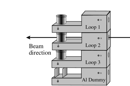
Figure 4: Representation of the cryogenic and dummy target assembly.

Localized target density fluctuations, induced by an intense incident beam, can modify significantly the average density of a cryogenic target. Uncertainties in target density enter directly as uncertainties in the total cross section, and can be current-dependent on a point-to-point basis. The current-dependence can be measured by comparing the yields at fixed kinematics with varying beam currents. The deadtime-corrected yields should be proportional to the luminosity (and, therefore, to the target density).

The result of such a ‘luminosity scan’ for E94-110 is shown in Fig. 5, where the luminosity relative to the lowest current has been plotted on the vertical axis. The error bars on the data are statistical only and do not reflect fluctuations in the beam current. The correction factor applied to the measured target density (at zero current) to account for the reduction resulting from localized target boiling is given by the product of the fitted slope and the current at which the data was taken. For the present data the current was typically kept at 60 $\pm$ 2 $\mu$A, resulting in a density correction of

$$(2.4\pm 0.2)\%\cdot 60\mu{\rm A}/100\mu{\rm A}=1.44\pm 0.12\%.$$ (8)

The uncertainty in the current did not contribute appreciably to the uncertainty on this correction. The total estimated run-to-run uncertainty in the target density is 0.1%.

Figure 5: Relative hydrogen target yield versus beam current.

IV.3 HMS Spectrometer

The HMS is a magnetic spectrometer consisting of a $25^{\circ}$ vertical bend dipole magnet (D) for momentum dispersion and three quadrupole magnets (Q1, Q2, Q3) for focusing. All magnets are superconducting and were operated in a mode to provide a point-to-point optical tune. A schematic side view of the HMS is shown in Fig. 6, and includes representations of the pivot (with target chamber), magnets, and the shielded hut containing the detector stack.

The detector stack is shown in Fig. 7 and consists of two vertical drift chambers baker (DC1 and DC2) for track reconstruction, scintillator arrays (S1X(Y) and S2X(Y)) for triggering, and a threshold gas Čerenkov and electromagnetic calorimeter, which were both used in the present experiment for particle identification (PID) and pion rejection.

The acceptance limits of the HMS in-plane ($Y^{\prime}$) and out-of-plane ($X^{\prime}$) scattering angles are defined by an octagonal collimator positioned between the target and the first quadrupole magnet. The edges of this collimator define a maximum angular acceptance of $-28~{}<~{}Y^{\prime}~{}<~{}28$ mrad and $-75~{}<~{}X^{\prime}~{}<~{}75$ mrad, and a total solid angle of about 6.8 msr. Additional details on the HMS can be found elsewhere dutta .

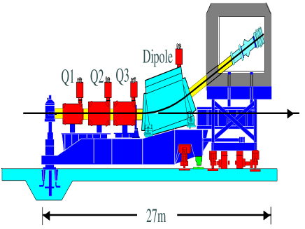
Figure 6: (Color online) Schematic drawing of the HMS spectrometer.

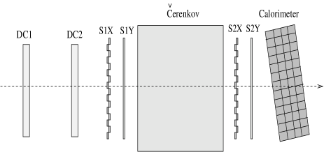
Figure 7: Schematic drawing of the HMS detector stack. The component detectors are described in the text.

IV.4 Data Acquisition

Data acquisition was performed using the CEBAF On-line Data Acquisition (CODA) software abbot1 running on a SUN Ultra-2 workstation. The detector information for each event was collected from the front-end electronics by VME/CAMAC computers (collectively referred to as Read-Out Controllers or ROCs). Event fragments from the ROCs were then transfered via TCP/IP to CODA, which formed events and wrote them to disk.

V Data Analysis

CODA events from individual run files where decoded by the Hall C Replay software, which reconstructed the trajectories of individual particles from hit information in the drift chambers. Tracks were then transported back to the target via an optical transport model of the HMS, which allowed the determination of the particle kinematics. For each run an HBOOK hbook ntuple was then created which contained the reconstructed event kinematics and calibrated PID detector information. The final analysis of the ntuples into experimental yields is described in the sections which follow.

V.1 Kinematic Calibrations

One of the larger $\varepsilon$-dependent uncertainties that directly affects Rosenbluth separations is that due to the uncertainties in the kinematics at which the cross sections are measured. It is convenient to absorb this uncertainty directly into the cross sections by calculating the expected difference in the measured cross section when the kinematics are changed from the nominal values within their uncertainties. In order to minimize this uncertainty, it was critical that the kinematic quantities, $E$, $E^{\prime}$, and $\theta$ be determined to the best possible precision. This was aided by the kinematic constraint of elastic scattering, that the reconstructed mass of the unmeasured hadronic state be equal to the proton mass.

For each kinematic setting, the difference of the reconstructed invariant mass, W, from the proton mass ($\Delta W$ = $W$ - $M_{p}$) was calculated after correcting for the effects of energy loss due to both ionization and bremsstrahlung emission. This provided a large set of kinematics for which the dependence of $\Delta W$ on possible energy and angle offsets could be studied. Finally a minimization of $\Delta W$ was performed to determine the best set of kinematic offsets under the following assumptions: 1) the offset of the nominal HMS central momentum from the true value was a constant fractional amount, and 2) the offset of the nominal HMS central angle from the true value was a constant. The nominal HMS momentum used in this study was that determined in  dutta , while the nominal HMS central angle was determined from a comparison of marks scribed on the floor of the Hall to a marker on the back of the spectrometer, which indicated the optical axis.

The reconstructed $W$ values for these data are plotted versus scattering energy in Fig. 8, for eight different beam energies and thirty one unique kinematic settings. It was found that the entire data set could be well described by assuming that the true HMS central angle was smaller than the nominal value by 0.6 mrad, and that the true HMS central energy was smaller than the nominal value by 0.39$\%$.

The true beam energy was also found to be smaller than the Arc measurements by an amount that varied with the energy. This latter result was subsequently confirmed mack by a remapping and analysis of the field for one of the Arc magnets. The reconstructed values for $W$ are shown, both before (open symbols) and after (solid symbols) correcting for the kinematic offsets found from these studies. The corrected values are all seen to be within 1-2 MeV of the proton mass. This procedure was used for the E94-110 data and yielded a estimated uncertainty in the corrected beam energy of 0.056$\%$, about half that typically quoted from Hall C Arc measurements. We estimate that this uncertainty is the quadrature sum of equal normalization and run-to-run uncertainties. We note that the beam energies determined from the Arc measurements utilizing the updated field maps agree with the current results to about 0.05%.

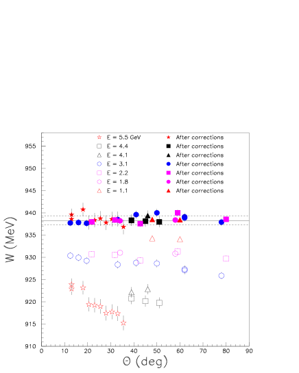
Figure 8: (Color online) Reconstructed $W$ vs. HMS central angle for elastic scattering kinematics. Open symbols represent data before kinematic corrections were applied, while the solid symbols represent the data after applying the calibration corrections.

V.2 Binning the Data

The data were binned on a 2-dimensional grid in the reconstructed variables $E^{\prime}$ and $\theta$. This was because, at fixed beam energy, the inclusive cross section only depends on the scattered electron energy and angle. In practice, the binning in $E^{\prime}$ was converted to a binning in $\delta P/P$, which is the more natural variable for the application of the acceptance corrections. The ranges were chosen such that the entire angular acceptance was included and the $\delta P/P$ acceptance was well determined from the model of the HMS. For $\delta P/P$, the binning chosen was 16 bins over a range of $\pm 8\%$, while for $\theta$ the binning chosen was 20 bins over a range of $\pm 35$ mrad ($\Delta\theta$ = 3.5 mrad). We note that the physical solid angle coverage ($\Delta\Omega$) can be different for each $\Delta\theta$.

V.3 Analysis Procedure

For a beam of electrons of energy $E$ incident on a fixed proton target, the number of electrons scattered at an angle $\theta$ in a solid angle $\Delta\Omega$ is related to the differential cross section, ${d\sigma(\theta)/d\Omega}$ by

$$N(\theta)=\mathcal{L}\cdot\frac{d\sigma(\theta)}{d\Omega}\Delta\Omega,$$ (9)

where $\mathcal{L}$ is the integrated luminosity. This is not the OPEA cross section of Equation 6, but contains contributions from higher order QED effects. These include virtual particle loops, multi-photon exchange, as well as the emission of bremsstrahlung photons, both before and after the scattering.

The emission of unmeasured bremsstrahlung photons by either the electron beam or the outgoing detected electron results in energies at the scattering vertex which are either smaller (the incoming case) or larger (the outgoing case) from those used in the reconstruction of the kinematics. This results in a large radiative “tail” in both the reconstructed $E^{\prime}$ and the invariant hadron energy distributions for elastic events. To compare to the OPEA cross section, requires that this radiative tail be integrated to some cut-off in $E^{\prime}$, with a correction factor, which included the remaining higher order effects, depending on this cut-off. This “radiative” correction is applied as a multiplicative factor (denoted RC) and is discussed in more detail in section V.8. Because the radiative tail extends beyond the threshold for single pion production at $W^{2}\approx 1.16$ $\rm GeV^{2}$, the integration was cutoff at $W^{2}_{max}<1.16$ $\rm GeV^{2}$ to avoid including events from inelastic processes. The corresponding correction factor, RC($W^{2}_{max}$), is therefore cutoff dependent.

In addition, the measured number of counts must also be corrected for detector efficiencies, $eff$, and the effective solid angle acceptance, $\Delta\Omega_{eff}(\theta,E^{\prime})$, after subtraction of counts from background processes, BG$(\theta,E^{\prime})$. In this experiment the measured cross section was determined for each bin on a 2-dimensional grid of the electron scattering energy and angle, $E^{\prime}$ and $\theta$, across the entire phase space for which the spectrometer has a non-zero acceptance. The extracted cross section was then determined from the relation,

$$\frac{d\sigma_{1\gamma}(\theta)}{d\Omega}=\frac{RC(W^{2}_{max})}{\mathcal{L}}{\int}^{W^{2}_{max}}{\it dE^{\prime}}\frac{[N(E^{\prime},\theta)-BG(E^{\prime},\theta)]}{eff\cdot\Delta\Omega_{eff}(E^{\prime},\theta)}.$$ (10)

The individual ingredients will be discussed in detail in the following sections.

V.4 Backgrounds

There are three physical processes that are possible sources of background counts to the elastically scattered electron yields. These are: electrons scattered from the target aluminum walls, negatively charged pions that are not separated from electrons by the PID cuts, and electrons originating from other processes, which are dominated by charge symmetric processes which produce equal numbers of positrons. Each of these potential backgrounds will be examined in the discussion that follows.

V.4.1 Target Cell Backgrounds

The quasielastic scattering from nucleons in aluminum nuclei can produce electrons at the same kinematics as those from elastic ep scattering. The scattering of the beam from front and back of the target cell wall produces backgrounds of this type which are difficult to isolate. Therefore, the corresponding background is determined by measuring the yield of events from a “dummy” target, which is a mockup of the target ends. In order to minimize the data acquisition time, the total thickness of this dummy target was about 8 times the total cell wall thickness seen by the beam. After measuring the dummy yield, the total background from scattering from the target walls, ${\rm BG}_{w}(E^{\prime},\theta)$, was then determined from

$${\rm BG}_{w}(E^{\prime},\theta)=\frac{t_{w}Q_{w}}{t_{d}Q_{d}}N_{d}(E^{\prime},\theta)\cdot C_{\rm br}(E^{\prime},\theta),$$ (11)

where $Q_{w(d)}$ is the total charge incident on the walls (dummy), $t_{w(d)}$ is the total thickness of the walls (dummy), and $N_{d}(E^{\prime},\theta)$ is the number of events collected for the dummy run after applying efficiency and deadtime corrections.

The factor, $C_{\rm br}(E^{\prime},\theta)$, corrects for the difference in external bremsstrahlung emission due to the greater thickness of the dummy target. More precisely, this accounts for the fact that the distribution of events for thicker targets are more strongly shifted toward lower scattering energies (higher $W$) than those for thinner targets. The size of this correction was studied and was found to be less than a few tenths of a percent at all kinematics measured, and typically less than $0.1\%$. Since this was the typical size of the uncertainty in this correction, we have taken $C_{\rm br}=1$, and absorbed an additional $0.1\%(0.1\%)$ into the point-to-point (normalized) uncertainty in the background subtraction.

The largest contribution to the uncertainties in the aluminum background subtraction comes from the uncertainties in the thickness of the cell wall of about $1.5\%$ dunne . However, the typical size of this background was on the order of $8\%$ of the total yield, which leads to an uncertainty on the subtracted yield of only $0.12\%$. This uncertainty is approximately independent of the kinematics and run conditions.

V.4.2 Pion Backgrounds

Figure 9: Distribution of the number of photoelectrons collected in the Čerenkov detector for elastic kinematics of $E$ = 2.2 GeV and $p$ = 1 GeV/$c$.

Figure 10: Distribution of the fractional energy deposition in the calorimeter for events both before (open area) and after(shaded area) applying a requirement of $>2$ photoelectrons in the Čerenkov detector.

The rejection of negatively charged pions was accomplished by placing requirements on both the number of Čerenkov photoelectrons collected and the energy deposition of the particle in the calorimeter. The count distribution of photoelectrons collected in the HMS Čerenkov at an HMS momentum of 1 GeV is shown in Fig. 9. For electrons, this is a Poisson distribution, with a mean of approximately 10 photoelectrons. For pions, the number of photoelectrons produced should be zero. However, pions can produce $\delta$-rays (electron knockout) in the materials immediately preceding the Čerenkov detector and some of these “knock-on” electrons can produce Čerenkov radiation, with the probability of $\delta$-ray production increasing with energy. With a requirement of more than 2 photoelectrons, this decreases the pion rejection factor from the maximum value of about $1000:1$ found at low energies. However, this doesn’t cause any significant pion contamination above this cut since the worst $\pi^{-}/e^{-}$ ratios are at low scattering energy where the rejection factor is the largest.

The fractional energy deposition in the calorimeter, both before (unshaded region) and after (shaded region) applying the Čerenkov requirement of $>2$ photoelectrons to select electrons, is shown in Fig. 10 for the four kinematics that exhibited the worst $\pi^{-}/e^{-}$ ratio. The fractional energy deposition of the particles is calculated by dividing the energy collected in a fiducial region about the track in the calorimeter by the momentum determined from the track reconstruction. Even for these worst cases, it is evident that the Čerenkov requirement alone does a good job of removing pions. To further insure a clean electron sample, a requirement that the fractional energy deposited in the calorimeter be greater than $0.7$ was also applied. The pion background after applying both the Čerenkov and calorimeter requirements is estimated to be less than $0.1\%$.

The Čerenkov efficiency, using a 2 photoelectron cut, was found to be $99.6\%$, independent of the energy. This is because the shape of the electron distribution does not depend on the particle’s energy, resulting in the same fraction of electrons in the tail being removed. This is not true for the calorimeter, since a fixed energy resolution results in an increase in the width of the electron fractional energy distribution at lower energies. The calorimeter cut efficiency decreases from a maximum of about $99.5\%$ at energies above 3 GeV to about $98.5\%$ at an energy of 0.6 GeV. The run-to-run uncertainties on the efficiencies were estimated from Gaussian fits of the distribution of efficiencies determined for each run from the entire E94-110 elastic data set, and were found to be $0.1\%$ for the Čerenkov detector and $0.1\%$ for the calorimeter.

V.5 Acceptance Corrections

Figure 11: HMS effective solid angle plotted in $\theta-\delta P/P$ space, using the binning described in the text.

Whether a scattered electron reaches the detector stack or is stopped by hitting the edge of the collimator or one of the various apertures in the HMS magnet system and beam pipe is dependent upon several factors, including: 1) the electron momentum, 2) the in-plane and out-of-plane scattering angles, and 3) the vertex position. However, the physics depends only upon the momentum and full scattering angle, $\theta=\cos^{-1}\left[\cos(X^{\prime})\cos(\theta_{c}-Y^{\prime})\right]$, so that for a fixed central spectrometer angle, $\theta_{c}$, it is convenient in what follows to consider only the $E^{\prime}$ and $\theta$ dependence of the acceptance averaged over the vertex coordinates.

Using a model of the spectrometer, the fractional acceptance, $A(E^{\prime},\theta)$, is calculated by generating Monte Carlo events and taking the ratio of the number of detected events to the number of generated events for each bin in phase space. That is

$$A(E^{\prime},\theta)\equiv N_{acc}(E_{gen}^{\prime},\theta_{gen})/N_{gen}(E_{gen}^{\prime},\theta_{gen}),$$ (12)

where $N_{gen}(E_{gen}^{\prime},\theta_{gen})$ is the number of events generated and $N_{acc}(E_{gen}^{\prime},\theta_{gen})$ is the number of events accepted in a given $(E_{gen}^{\prime},\theta_{gen})$ bin. The $gen$ subscripts denote that the kinematics used for the binning are as generated. The fractional acceptance as defined here is simply a probability. However, it is evident that $A(E^{\prime},\theta)$ depends upon the solid angle, $\Delta\Omega_{gen}(\theta)$, into which events are generated. The “effective” solid angle coverage for each 2-dimensional bin is

$$\Delta\Omega_{eff}(E^{\prime},\theta)\equiv A(E^{\prime},\theta)\cdot\Delta\Omega_{gen}(\Delta\theta),$$ (13)

and is independent of the size of $\Delta\Omega_{gen}(\Delta\theta)$. For example, increasing the generation limits of the out-of-plane angle, $X^{\prime}$, from $\pm 100$ mrad to $\pm 150$ mrad will decrease $A(E^{\prime},\theta)$ since $\left|X^{\prime}\right|>100$ mrad is already outside of the collimator aperture. However, $\Delta\Omega_{gen}(\Delta\theta)$ will increase accordingly and $\Delta\Omega_{eff}$ will remain unchanged.

We note that the determination of $A(E^{\prime},\theta)$ does not require generating the events uniformly provided that the number generated in each part of phase space is known. The assumption here is that events generated in a given $(E^{\prime},\theta)$ bin are not detected in another $(E^{\prime},\theta)$ bin. The fractional acceptance as defined is then simply the probability that an event generated in a given bin will be detected in that bin, and, therefore, the correction to the yield due to the fractional acceptance in each bin is $1/A(E^{\prime},\theta)$. If the bin-to-bin migration is small then it is already approximately accounted for by redefining the acceptance in Equation 12 to

$$A(E^{\prime},\theta)=N_{acc}(E_{rec}^{\prime},\theta_{rec})/N_{gen}(E_{gen}^{\prime},\theta_{gen}),$$ (14)

where the $rec$ subscripts denote the kinematics as reconstructed. The $\Delta\Omega_{eff}$ distribution extracted from the HMS model for $E^{\prime}$ = 2.8 GeV and $\theta_{c}=12.5^{\circ}$ is shown in figure 11. The shape in $\theta-\theta_{c}$ is dominated by the octagonal collimator, which largely determines the HMS solid angle acceptance. We note that the acceptance is not symmetric in the full scattering angle when the out-of-plane angle contributes significantly (i.e. at forward in-plane spectrometer angles), even though the HMS has a high degree of symmetry about the in-plane scattering angle. This is because any out-of-plane angle will always result in a larger full scattering angle.

The solid angle defined by the HMS collimator is about 6.75 msr for a point target. This is slightly reduced for a 4 cm extended target and the reduction becomes larger as the spectrometer is moved to larger angles. At the smallest angle measured of $\theta_{c}=12.5^{\circ}$, the average solid angle acceptance due to the collimator for a momentum bite of $\left|\delta p/p\right|<8\%$ was determined from the HMS model to be 6.714 msr. The reduction due to all other apertures resulted in a further reduction of only 2.5% to 6.612 msr. At the largest angle measured of $\theta_{c}=80^{\circ}$, the average solid angle acceptance due to the collimator was determined to be 6.685 msr, with a further reduction due to other apertures of 5.2% to 6.335 msr. For this momentum bite the largest reduction of events after the collimator is in the second quadrupole.

The normalization uncertainty on the acceptance corrections was estimated by combining in quadrature an uncertainty of 0.7% stemming from the reduction in solid angle due to apertures other than the collimator (more than one fourth the total at $\theta_{c}=12.5^{\circ}$) and an uncertainty of 0.4% due to the modeling of the HMS optics.

The optical properties of the HMS have been well studied dutta utilizing several techniques and a large amount of dedicated optics data taken during many experiments over nearly a decade. For the HMS, the optical transport of charged particles through the spectrometer is independent of the momentum setting to a very high degree. The $\Delta\Omega$ distribution at a given $\theta_{c}$ is then only dependent on the energy setting through the dependence of the resolution (including energy straggling) and multiple scattering effects in the spectrometer.

V.6 Elastic Peak Integration

As already noted, the scattering energy distribution of the elastic peak at an individual $\theta$ value is broadened from the $\delta$ function expected in the OPEA due to several effects. These include energy resolution effects, and energy loss due to both ionization and bremsstrahlung emission. A typical peak distribution for a single $\theta$ bin is shown in Fig. 12. The lower limit of integration is chosen to both minimize the loss of events due to resolution smearing and to minimize the sensitivity to potential backgrounds, while the upper limit is chosen to include as much of the peak as possible yet to be below the threshold for inelastic $\pi$ production at $W^{2}\approx 1.16$ $\rm GeV^{2}$.

The sensitivities to both the lower and upper limits were studied and were found to be small. For the lower limit, the insensitivity indicates that the aluminum background subtractions are correctly handled. For the upper limit, it indicates that both the resolution effects and the shape of the bremsstrahlung distribution are accounted for reasonably well. Once the upper limit has been chosen, the fraction of the distribution that is outside this limit is accounted for by the correction factor RC($W^{2}_{max}$). If the effects of bremsstrahlung, energy straggling, and resolution are well understood, then a corresponding peak integration should be independent of the energy cutoff chosen, once the corresponding radiative correction has been applied.

The sensitivity of the extracted cross section to the energy cutoff is shown in Fig. 13. For each kinematic setting, the ratio of the integrated distribution for an energy cutoff of $W^{2}_{max}$ to that for a cutoff of $1.15$ $\rm GeV^{2}$ is plotted versus $\varepsilon$. In the upper plot $W^{2}_{max}=1.10$ $\rm GeV^{2}$, in the middle plot $W^{2}_{max}=1.05$ $\rm GeV^{2}$, and for the bottom plot $W^{2}_{max}=1.0$ $\rm GeV^{2}$. The typical point-to-point difference in tail-corrected integration is less than $0.3\%$ for the largest change in the cutoff value and shows little $\varepsilon$ dependence. We take this as the estimated random point-to-point uncertainty on this procedure and include it in the uncertainty of the radiative corrections. Additionally, we note that the normalization difference of about 1% between between the smallest and largest values for $W^{2}_{max}$ is likely due to a combination of unoptimized resolution matching and the approximate handling of the energy straggling in the simulation used for generating the acceptance corrections. However, this optimization becomes much less important as more of the peak is integrated. We take 0.35% as the estimated normalization uncertainty on this procedure and include it in the uncertainty of the radiative corrections.

Finally, we note that, except for the three measurements at beam energies below 2 GeV, the same $W^{2}_{max}$ value was used for all kinematic settings. This was possible because of the large acceptance of the HMS spectrometer. This is in contrast to previous precision measurements walker ; andiv , in which the spectrometer acceptance determined the maximum $W^{2}_{max}$ at each kinematic setting.

Figure 12: Sample $W^{2}$ count distribution measured for elastically scattered electrons in a single $\theta$ bin after subtraction of the Al quasielastic contribution determined from the dummy target.

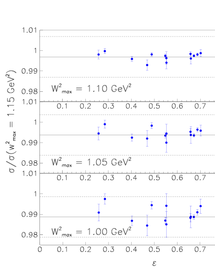
Figure 13: (Color online) Ratio of the cross section calculated with a cutoff in the tail integration of $W^{2}$ = 1.10 $\rm GeV^{2}$ (top), $W^{2}$ = 1.05 $\rm GeV^{2}$ (middle), and $W^{2}$ = 1.0 $\rm GeV^{2}$ (bottom), relative to a cutoff of $W^{2}$ = 1.15 $\rm GeV^{2}$.

V.7 $\theta$ Bin-Centering and Averaging

After performing the peak integration, the cross section is then extracted for each $\theta$ bin. Often, the statistics taken in each bin are small ($<$ 2000 counts). In order to improve the statistical accuracy, one would like to combine the data from all $\theta$ bins. If the cross section did not depend (or depended only linearly) on the scattering angle, the cross sections extracted in each bin could simply be averaged. This is not the case, however. The HMS spectrometer has a relatively large acceptance of about $\pm$1.8 degrees in the scattering angle. Therefore, the cross section can vary greatly across the angular acceptance. At some kinematics, this variation can be a factor of 3 or more (and strongly non-linear) across the acceptance. In order to average the cross sections in each $\theta$ bin, the $\theta$ dependence of the cross section must be corrected for.

This correction is called “$\theta$ bin-centering” (BC), and our prescription for it is straightforward. Since we would like to quote the cross section at the central angle of the spectrometer, the following correction is applied to each $\theta$ bin:

$$\left[\frac{d\sigma(\theta)}{d\Omega}\right]_{BC,i}=\frac{d\sigma(\theta_{i})}{d\Omega}\cdot\frac{\sigma^{Mod}(\theta)}{\sigma^{Mod}(\theta_{i})},$$ (15)

where $\theta$ is the central angle, $\theta_{i}$ is the angle for the $i^{th}$ bin, and $\sigma^{Mod}$ is the value of a cross section model. For this procedure to be valid, care must be taken to subtract all backgrounds and to apply all corrections that have a $\theta$ dependence, bin-by-bin. This includes radiative corrections. The bin-centered cross sections can then be averaged over the $\theta_{i}$ to give the measured cross section at the central spectrometer angle. This was done as a weighted average, where the inverse of the square of the full statistical errors was used as a weighting factor. The statistical errors take into account the statistics of both the hydrogen and subtracted target endcap events, as well as the acceptance correction uncertainties due to statistical errors on the Monte Carlo generation.

An example of this procedure is presented in Fig. 14. Shown is the cross section extracted at a beam energy of 3.12 GeV and a central HMS angle of $12.5^{\circ}$, before both acceptance and BC corrections (triangles). Also plotted is the cross section after applying acceptance corrections (squares) and after applying both acceptance and bin-centering corrections (circles). Only statistical uncertainties in the data are included in the error bars shown. However, the calculated acceptance corrections for bins at the edge of the acceptance can have large fractional errors, as they are very sensitive to both accurate modeling of the multiple scattering processes and small variations in the positions of apertures like the collimator. To minimize the effects of such sensitivities, bins at the edge of the $\theta$ acceptance where the calculated acceptance was below some minimum value were neglected in the averaging procedure. The angular acceptance limits used in the present experiment are represented by the vertical dashed lines in Fig. 14. The cross sections obtained after averaging over these limits were found to be quite insensitive to the effects described above. Uncertainties associated with these effects were studied by adjusting aperture/target positions, magnet fields, and multiple scattering distributions within reasonable limits and determining the corresponding acceptance function. The cross section extracted with this acceptance function was typically found to agree with that using the nominal acceptance function to within 0.5%.

The shape of the uncorrected distribution is the convolution of the $\theta$ dependence of the cross section with the acceptance of the spectrometer, with the latter being primarily defined by the collimator. Correcting for the acceptance leaves only the $\theta$ dependence, which is then removed by the bin-centering corrections. The resulting, fully corrected, cross section should then be a constant across the $\theta$ acceptance and equal to the cross section at the central $\theta$ to within statistical fluctuations. This is indeed the case, allowing for small variations which are mostly due to an imperfect optics model for the spectrometer, as well as the approximate treatment of the multiple scattering effects in the simulations.

Figure 14: Cross section extracted in each $\theta$ bin across the HMS acceptance. The various data are discussed in the text.

V.8 Radiative Corrections

Figure 15: Feynman diagrams for higher order QED processes, including (a) vacuum polarization, (b) vertex corrections, (c) two photon exchange, and (d) internal bremsstrahlung emission from electrons. Not shown are diagrams for proton bremsstrahlung, or external bremsstrahlung.

While the form factors can be easily extracted from the Born cross section for single photon exchange, the cross section that is measured in a scattering experiment includes higher order electromagnetic processes which are depicted in Fig. 15. These processes can be categorized into two types: 1) the internal processes, which originate due to the fields of the particles at the scattering vertex, and 2) the external processes, which originate due to the fields of particles in the bulk target materials. The internal processes include: vacuum polarization, vertex corrections, two-photon exchange, and (internal) bremsstrahlung emission in the field of the proton from which the scattering took place, while the external process is due to (external) bremsstrahlung in the field of a proton in the material either before or after the scattering vertex.

The radiative correction factors, which account for these higher order processes, were calculated using the same procedure as the high precision SLAC data walker ; andiv and discussed in detail in Reference walker . This procedure is based on the prescription of Mo and Tsai tsai ; motsai . The radiative correction (RC) is applied to the measured cross section (after integration of the bremsstrahlung tail) as a multiplicative factor, i.e.,

$$\left[\frac{d\sigma(\theta)}{d\Omega}\right]_{Born}=RC\cdot\left[\frac{d\sigma(\theta)}{d\Omega}\right]_{Meas}.$$ (16)

The corrections calculated include only the infrared divergent contributions from the two-photon exchange and proton vertex diagrams, with the non-divergent contributions having been previously estimated motsai to be less than 1$\%$. However, the topic of two-photon exchange has recently been of renewed theoretical interest 2pho1 ; 2pho2 ; 2pho3 in light of the discrepancy between the elastic form factor ratios extracted from Rosenbluth separations of cross section measurements and those measured in polarization transfer experiments. In addition, a recent study positrons of the world’s data on the ratio of elastic cross sections for $e^{+}p$ to $e^{-}p$ has recently been made to look for evidence of two-photon effects.

The radiative corrections applied at each kinematic setting are listed in Table 3. We note that these correction factors are significantly smaller than those applied in References walker ; andiv . This is mostly due to integrating more of the radiative tail, but also to the reduction of external bremsstrahlung afforded by our much shorter target.

The uncertainties in the radiative correction procedure were studied in References walker ; andiv and were estimated to be 0.5% point-to-point and 1.0% nomalized. To these we have added, in quadrature, the additional contributions resulting from the radiative tail integration, which are discussed in Section V.6. .

V.9 Additional Corrections Applied to Large $E^{\prime}$ Data

The four cross section measurements at scattering energies greater than 3.5 GeV (indicated with a $\star$ in Table 3) required two additional corrections that were not needed for the rest of the data set. These corrections, which will be discussed in what follows, account for the following two effects: 1) an additional change in the effective target density, and 2) a small misfocusing in the spectrometer optics, relative to nominal.

During the data taking it was discovered that the fan controlling the flow of hydrogen through the cryogenic target had been inadvertently lowered from the 60 Hz nominal speed to 45 Hz. This resulted in larger localized boiling due to the beam and effectively lowered the density of hydrogen. To account for this, high statistics runs ($\approx 0.1\%$) were performed at both fan speeds and the size of the effect was determined from the ratio of cross sections. Since the effect of target boiling was already measured for a fan speed of 60 Hz, an additional correction to the yields of $+0.6\%\pm 0.2\%$ was included for the data taken at the lower speed.

In addition to the correction for the difference in target density, the cross section measurements at large $E^{\prime}$ were also corrected for a slight misfocusing of the spectrometer. A TOSCA tosca model of the HMS dipole indicated that it would start to suffer from saturation effects starting at currents corresponding to a momentum of 3.5 GeV for the central ray and that this effect would increase quadratically with momentum. This correction was included when setting the current in the dipole for this experiment, but was later found from both kinematic and optics studies to not be needed. These studies indicated that the actual HMS field continues to increase linearly with current to a high accuracy up to the highest momentum tested of 5.1 GeV.

The missetting of the dipole field due to this unneeded saturation correction resulted in reconstructing the wrong scattering angle by an amount that varied across the angular acceptance, and led to a depletion of events that reconstructed in the region of the angular acceptance used in the analysis. The correction to the reconstructed scattering angle was determined by requiring $W=M_{p}$ for each $\theta$ bin, and this correction was then fit as a function of $\theta$ across the angular acceptance. The result of this fit was applied as a correction to the scattering angle event-by-event, and effectively reshuffled events back into the depleted bins. The effect of this correction on the cross section was largest at the highest scattering momentum in this experiment of 4.7 GeV and resulted in a $1.6\%$ increase. The uncertainty on this correction was estimated to be $0.4\%$ and was assumed to be the same at all four kinematics where a correction was applied.

VI Systematic Uncertainties

The estimated systematic uncertainties for the experiment are listed in Table 1 for those that are assumed random point-to-point in $\varepsilon$ and in Table 2 for those that effect the overall normalization uncertainty only. The quadrature sum of the point-to-point and normalization uncertainties gives the absolute uncertainties on the cross section measurements. The point-to-point uncertainties are those that depend upon variable run conditions or kinematics. Discussions of the uncertainties presented here can be found in earlier sections of the text.

Table 1: E94-110 point-to-point systematic uncertainties.

Experimental Quantity	Uncertainty	$\Delta\sigma/\sigma$
		(pt-pt)
Beam Energy	$4\cdot 10^{-4}$	0.0024
Scattering Angle	0.2 mrad	0.0026
Target Density	0.1%	0.001
Target Length	0.1%	0.001
Beam Charge	0.2%	0.002
Acceptance	0.5%	0.005
Detector Efficiency	0.15%	0.0015
Tracking Efficiency	0.25%	0.0025
Deadtime Corrections	0.14%	0.0014
Target Cell Background	0.2%	0.002
Radiative Corrections	0.6%	0.006
	Total	0.0097

Table 2: E94-110 normalization uncertainties.

Experimental Quantity	Uncertainty	$\Delta\sigma/\sigma$
		(Norm)
Beam Energy	$4\cdot 10^{-4}$	0.0024
Scattering Angle	0.4 mrad	0.0053
Target Density	0.4%	0.004
Target Length	0.3%	0.003
Beam Charge	0.33%	0.0033
Acceptance	0.8%	0.008
Detector Efficiency	0.4%	0.004
Tracking Efficiency	0.3%	0.003
Deadtime Corrections	0.1%	0.001
Target Cell Background	0.3%	0.003
Radiative Corrections	1.1%	0.011
	Total	0.017

VII Results

Table 3: Table of measured ep elastic cross sections. The systematic uncertainties listed are the estimated point-to-point uncertainties for each kinematic setting. In addition there is scale uncertainty of 1.7%.

$E_{beam}$	$\Theta$	$Q^{2}$	$\varepsilon$	$\sigma$	$\Delta\sigma$ (stat)	$\Delta\sigma$ (sys)	RC
(GeV)	(Deg)	$({\rm GeV}/c)^{2}$		($\mu$b/sr)	($\mu$b/sr)	($\mu$b/sr)
1.148	47.97	0.6200	0.6824	0.1734E-01	0.35E-04	0.16E-03	1.055
1.148	59.99	0.8172	0.5492	0.4813E-02	0.11E-04	0.45E-04	1.047
1.882	33.95	0.8995	0.8104	0.1464E-01	0.28E-04	0.14E-03	1.098
2.235	21.97	0.6182	0.9187	0.1098E+00	0.40E-03	0.11E-02	1.120
2.235	31.95	1.1117	0.8226	0.8938E-02	0.25E-04	0.86E-04	1.121
2.235	42.97	1.6348	0.6879	0.1184E-02	0.54E-05	0.11E-04	1.114
2.235	58.97	2.2466	0.4885	0.1522E-03	0.86E-06	0.14E-05	1.100
2.235	79.97	2.7802	0.2843	0.2868E-04	0.21E-06	0.27E-06	1.083
3.114	12.47	0.4241	0.9740	0.8968E+00	0.25E-02	0.96E-02	1.150
3.114	15.97	0.6633	0.9553	0.1892E+00	0.80E-03	0.20E-02	1.151
3.114	19.46	0.9312	0.9308	0.4802E-01	0.12E-03	0.49E-03	1.154
3.114	32.97	2.0354	0.7835	0.1017E-02	0.26E-05	0.99E-05	1.154
3.114	40.97	2.6205	0.6726	0.2125E-03	0.74E-06	0.20E-05	1.150
3.114	49.97	3.1685	0.5480	0.5568E-04	0.28E-06	0.53E-06	1.147
3.114	61.97	3.7261	0.4026	0.1487E-04	0.10E-06	0.14E-06	1.137
3.114	77.97	4.2330	0.2574	0.4260E-05	0.49E-07	0.40E-07	1.121
4.104	38.97	3.7981	0.6578	0.4919E-04	0.31E-06	0.47E-06	1.185
4.104	45.96	4.4004	0.5528	0.1582E-04	0.29E-06	0.15E-06	1.181
4.413	44.98	4.7957	0.5526	0.1098E-04	0.20E-06	0.11E-06	1.192
4.413	50.99	5.2612	0.4686	0.4898E-05	0.73E-07	0.47E-07	1.188
$\star$5.494	12.99	1.3428	0.9655	0.4055E-01	0.11E-03	0.50E-03	1.214
$\star$5.494	17.96	2.2878	0.9239	0.2866E-02	0.13E-04	0.33E-04	1.220
$\star$5.494	20.47	2.7822	0.8955	0.9824E-03	0.41E-05	0.11E-04	1.223
$\star$5.494	22.97	3.2682	0.8627	0.3770E-03	0.15E-05	0.42E-05	1.226
5.494	25.47	3.7385	0.8261	0.1608E-03	0.14E-05	0.18E-05	1.226
5.494	27.97	4.1867	0.7865	0.7749E-04	0.61E-06	0.77E-06	1.228
5.494	32.97	5.0031	0.7023	0.2149E-04	0.23E-06	0.21E-06	1.226
5.494	35.48	5.3699	0.6593	0.1267E-04	0.20E-06	0.12E-06	1.225

The complete set of Born cross sections extracted from these precision elastic scattering measurements are listed in Appendix A. In total, measurements at 28 different kinematics were included in the final data set, covering a range in $Q^{2}$ from approximately 0.4 GeV to 5.5 GeV. In addition, a significant range in $\varepsilon$ was covered, even though the elastic kinematics were not specifically optimized for Rosenbluth separations.

VII.1 Comparisons to Fits of the Existing World’s Data

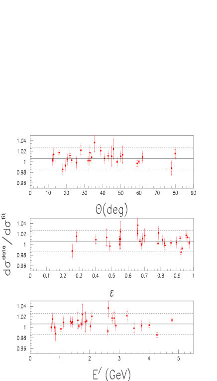
Figure 16: (Color online) The ratio of measured ep elastic cross sections to the Arrington fit of previous cross section data, as a function of scattering angle, longitudinal photon polarization, and scattering energy. The solid line indicates the average ratio of 1.006 and the dashed lines indicate $\pm 2\%$ of this value.

Comparisons of these cross sections were made to recent fits of the previous world’s data set. These included the fit of Brash $et$ al. from brash and the fits of Arrington from arrington . Both analyzes performed a fit to the combined cross section and polarization transfer data, while that of Arrington also included a fit to the cross section data alone. It should be stressed that, although nearly the same data sets were included in the fits, the method of combining the polarization transfer data differed.

In the work of Brash $et$ al., the polarization transfer results for the $Q^{2}$ dependence of $G_{E}/G_{M}$ were used as a constraint to do a one-parameter refit of the Rosenbluth data, from which $G_{M}$ was extracted. A $\chi^{2}$ minimization was then performed to fit $G_{M}$ as a function of $Q^{2}$. In the work of Arrington, two fits were performed: one that included the polarization transfer data, and one that did not. However, here the polarization transfer results for $G_{E}/G_{M}$ were included with the cross section measurements as equally weighted points in a $\chi^{2}$ minimization to fit both form factors simultaneously. This follows closely the older work of Walker walker on global fits to cross section data.

The ratio of the data to the Arrington fit of cross section data is shown in Fig. 16 versus $\theta$, $\varepsilon$, and $E^{\prime}$. The inner error bars represent the purely statistical uncertainties, while the full error bars include the point-to-point uncertainties as well. This fit is observed to describe the data set very well over the entire kinematic range. The $\chi^{2}$ (calculated using only the point-to-point uncertainties and after removing the average $0.6\%$ normalization difference between the current data set and the previous world data set of cross section measurements) distribution was found to be well described by a Gaussian distribution with a width corresponding to an average uncertainty of about 1.0$\%$, consistent with the estimated errors combining the systematic point-to-point and statistical uncertainties in quadrature. For each of the three fits previously described, the total $\chi^{2}$ per degree of freedom ($\chi^{2}_{\nu}$) to the data was calculated. The results for the region above $Q^{2}$ = 1 $({\rm GeV}/c)^{2}$, where the discrepancy between the cross section and polarization results differ significantly, were found to be $\chi^{2}_{\nu}=$ 0.76 (Arrington fit to cross sections), 1.06 (Arrington fit including polarization transfer results), and 2.95 (Brash $et$ al fit), allowing the overall normalization to vary.

These results are interesting for two reasons. Firstly, the full data set above $Q^{2}$ = 1 $({\rm GeV}/c)^{2}$ favor the fit to cross section data only over the fits that includes the polarization transfer data. Secondly, the data favor the Arrington prescription for combining the cross section and polarization transfer data over the prescription of Brash $et$ al. This does not resolve the inconsistency between the Rosenbluth and polarization transfer results, but rather underscores a consistency in the global cross section data set including these new measurements. The discrepancy with these and the polarization transfer measurements is highlighted further.

VII.2 Rosenbluth Extractions of Form Factors

Figure 17: Rosenbluth separations of the form factors. Plotted is the reduced cross sections ($\times 1000$) versus $\varepsilon$.

The individual Sachs form factors were extracted from the cross section data at seven different $Q^{2}$ values via the Rosenbluth separation method. This required that the cross section measurements at similar $Q^{2}$ values be grouped. Since none of the measurements were taken at precisely the same $Q^{2}$, a correction factor was applied to some of the cross sections in each group to evolve to a common $Q^{2}$. The correction factor for this $Q^{2}$ evolution was calculated from fits to previous data via

$$\frac{d\sigma(Q^{2}_{c},\varepsilon)}{d\Omega}=\frac{d\sigma(Q^{2},\varepsilon)}{d\Omega}\cdot\frac{\sigma^{Mod}(Q^{2}_{c},\varepsilon)}{\sigma^{Mod}(Q^{2},\varepsilon)},$$ (17)

where $\sigma^{Mod}$ is the value given by the fit of Arrington to the cross sections data, and $Q^{2}$, $Q^{2}_{c}$, represent the values before and after the evolution, respectively.

In order to perform Rosenbluth separations at a particular $Q^{2}$, the following two conditions on the data were required: 1) each separation must contain three distinct $\varepsilon$ points, and 2) the $Q^{2}$ evolution for each $\varepsilon$ point must constitute less than a 15$\%$ correction. The sensitivity of the extracted form factors on the model used for the $Q^{2}$ evolution was found to be much less than the uncertainties. Plots of the reduced cross sections versus $\varepsilon$ are presented in Fig. 17 for each $Q^{2}$. Also presented are the results of the linear fit. The error bars on each point represent the total point-to-point uncertainties, including both statistical and systematic uncertainties added in quadrature.

Table 4: Table of the Rosenbluth extracted Sachs form factors relative to the dipole form factor, $G_{d}=\frac{1}{(1+Q^{2}/0.71)^{2}}$ ($Q^{2}$ in $({\rm GeV}/c)^{2}$.

$Q^{2}$	${G_{M}}_{p}/(\mu_{p}G_{dip})$	${G_{E}}_{p}/G_{dip}$	$\mu{G_{E}}_{p}/{G_{M}}_{p}$
$({\rm GeV}/c)^{2}$
0.65	0.968 $\pm$ 0.032	1.035 $\pm$ 0.052	1.069 $\pm$ 0.085
0.91	1.028 $\pm$ 0.019	0.954 $\pm$ 0.053	0.928 $\pm$ 0.067
2.20	1.050 $\pm$ 0.016	0.923 $\pm$ 0.121	0.878 $\pm$ 0.125
2.75	1.055 $\pm$ 0.010	0.888 $\pm$ 0.114	0.841 $\pm$ 0.109
3.75	1.044 $\pm$ 0.015	0.873 $\pm$ 0.232	0.837 $\pm$ 0.220
4.20	1.012 $\pm$ 0.012	1.255 $\pm$ 0.157	1.240 $\pm$ 0.163
5.20	1.007 $\pm$ 0.032	1.183 $\pm$ 0.511	1.176 $\pm$ 0.552

The results for the ratio $\mu{G_{E}}/{G_{M}}$ extracted from the current data set are presented in Fig. 18, along with previous extractions from both cross section walker and polarization transfer jones ; gayou1 data. The current data are seen to agree well with the previous cross section data, while being in significant disagreement with the polarization transfer results. The error bars on each point represent the uncertainties obtained for the fit parameters, while the hatched band at the top of the figure represents that due to the estimated 0.4 mrad uncertainty in the absolute scattering angle. To a large degree, an error in the scattering angle would shift the entire set of ratios up or down but would not significantly alter the trend versus $Q^{2}$, which is significantly different from that of the polarization transfer data.

Figure 18: (Color online) Extracted values of $\mu{G_{E}}/{G_{M}}$. Also shown are those extracted from previous Rosenbluth and polarization transfer measurements. The error bars on the data include the full point-to-point uncertainties, while the hatched band at the top indicates the uncertainty due to the absolute uncertainty in the scattering angle of 0.4 mrad.

VIII Conclusion

We have performed high precision measurements of the ep elastic cross section covering a considerable amount of the $Q^{2}-\varepsilon$ space for which there exists a large discrepancy between Rosenbluth and polarization transfer extractions of the ratio $\mu{G_{E}}/{G_{M}}$. This data set shows good agreement with previous cross section measurements, indicating that if a here-to-fore unknown systematic error does exist in the cross section measurements then it is intrinsic to all such measurements.

A likely candidate, which has received much theoretical interest recently 2pho1 ; 2pho2 ; 2pho3 , is possible contributions from two-photon exchange, which are not fully accounted for in the standard radiative corrections procedure of Mo-Tsai. Although it is currently unclear whether such an effect can fully explain the discrepancy, considerable progress is being made.

Complementary to this theoretical effort is the recently completed experiment super in JLab Hall A which utilizes the so-called ‘Super-Rosenbluth’ technique to extract the form factor ratio. This experiment measured the proton cross sections and is therefore sensitive to a different set of systematic uncertainties than the previous electron cross section data. However, these measurements are still as sensitive to two-photon exchange effects as electron cross section measurements and will, therefore, provide a vital clue whether such effects are present. In any event, it is critical that the source of the discrepancy be found if there is to be any hope of extracting the $Q^{2}$ dependence of the individual form factors.

- (1) M. K. Jones et al., Phys. Rev. Lett. 84, 1398 (2002).
- (2) O. Gayou et al., Phys. Rev. Lett. 88, 092301 (2002).
- (3) O. Gayouet al., , Phys. Rev. C 64, 038202 (2001).
- (4) A.I. Akhiezer and M.P. Rekalo, Sov. J. Part. Nucl. 3, 277 (1974).
- (5) R. G. Arnold, C.E. Carlson, and F. Gross, Phys. Rev. C 23, 363 (1981).
- (6) J. Litt et al., Phys. Lett. B31, 40 (1970).
- (7) L.E. Price, J.R. Dunning, M. Goitein, K. Hanson, T. Kirk, and R. Wilson, Phys. Rev. D 4, 45 (1971).
- (8) R. C. Walker et al., Phys. Rev. D 49, 5671 (1994).
- (9) L. Andivahis et al., Phys. Rev. D 50, 5491 (1994).
- (10) M. N. Rosenbluth, Phys. Rev. 79, 615 (1956).
- (11) E. J. Brash, A. Kozlov, S. Li, and G. M. Huber, Phys. Rev. C 65, 051001 (2002).
- (12) J. Arrington, Phys.Rev. C 68, 034325 (2003).
- (13) J. Arrington, Phys.Rev. C 69, 022201 (2004).
- (14) W. Bartel et al., Nucl. Phys. B58, 429 (1973).
- (15) Ch. Berger et al., Phys. Lett. 35B, 87 (1971).
- (16) P. E. Bosted, Phys. Rev. C 51, 409 (1994).
- (17) A. F. Sill et al., Phys. Rev. D 48, 29 (1993).
- (18) C. S. Armstrong, Ph.D. Thesis, College of William and Mary (1998).
- (19) J. Dunne, “ 94-110 Target Worksheet”, Jefferson Lab Internal Report (2001).
- (20) O.K. Baker et al., Nucl. Instrum. Meth. A367, 92 (1995).
- (21) Y. S. Tsai, Phys. Rev. 122, 1898 (1961).
- (22) L. W. Mo and Y.S. Tsai, Rev. Mod. Phys. 41, 205 (1969).
- (23) J. Arrington, nucl-ex/0311019.
- (24) D. J. Abbott et al., Proceedings of the 1995 IEEE Conference on Real-Time computer Applications in Nuclear, Particle, and Plasma Physics (May 1995), pp. 147-151.
- (25) Vector Fields Ltd., 24 Banksike, Kidlington, Oxford OX5 1JE, England.
- (26) D. Dutta et al., Phys.Rev. C 68, 064603 (2003).
- (27) C. E. Keppel, et al., Jefferson Lab experiment E94-110, 1994.
- (28) D. Mack, (private communication).
- (29) HBOOK Reference Manual, V4.20, Application Software Group, Computing and Networking Division (1995), CERN Geneva (1999).
- (30) P. G. Blunden, W. Melnitchouk, and J. A. Tjon, Phys. Rev. Lett. 91, 142304 (2003).
- (31) P. A. M. Guichon and M. Vanderhaeghen, Phys. Rev. Lett. 91, 142303 (2003).
- (32) M. P. Rekalo and E. Tomasi-Gustafsson (2003), nucl-th/0307066.
- (33) J. Arrington, R. E. Segel et al., Jefferson Lab experiment E01-001, 2001.