The dynamics of the quasielastic ¹⁶O$\bm{(e,e^{\prime}p)}$ reaction at $\bm{Q^{2}}$ $\approx$ 0.8 (GeV/$\bm{c}$)²

Abstract

The physics program in Hall A at Jefferson Lab commenced in the summer of 1997 with a detailed investigation of the ¹⁶O$(e,e^{\prime}p)$ reaction in quasielastic, constant $(q,\omega)$ kinematics at $Q^{2}$ $\approx$ 0.8 (GeV/$c$)², $q\approx$ 1 GeV/$c$, and $\omega\approx$ 445 MeV. Use of a self-calibrating, self-normalizing, thin-film waterfall target enabled a systematically rigorous measurement. Five-fold differential cross-section data for the removal of protons from the $1p$-shell have been obtained for 0 $<$ $p_{\rm miss}$ $<$ 350 MeV/$c$. Six-fold differential cross-section data for 0 $<$ $E_{\rm miss}$ $<$ 120 MeV were obtained for 0 $<$ $p_{\rm miss}$ $<$ 340 MeV/$c$. These results have been used to extract the $A_{LT}$ asymmetry and the $R_{L}$, $R_{T}$, $R_{LT}$, and $R_{L+TT}$ effective response functions over a large range of $E_{\rm miss}$ and $p_{\rm miss}$. Detailed comparisons of the $1p$-shell data with Relativistic Distorted-Wave Impulse Approximation (rdwia), Relativistic Optical-Model Eikonal Approximation (romea), and Relativistic Multiple-Scattering Glauber Approximation (rmsga) calculations indicate that two-body currents stemming from Meson-Exchange Currents (MEC) and Isobar Currents (IC) are not needed to explain the data at this $Q^{2}$. Further, dynamical relativistic effects are strongly indicated by the observed structure in $A_{LT}$ at $p_{\rm miss}$ $\approx$ 300 MeV/$c$. For 25 $<$ $E_{\rm miss}$ $<$ 50 MeV and $p_{\rm miss}$ $\approx$ 50 MeV/$c$, proton knockout from the $1s_{1/2}$-state dominates, and romea calculations do an excellent job of explaining the data. However, as $p_{\rm miss}$ increases, the single-particle behavior of the reaction is increasingly hidden by more complicated processes, and for 280 $<$ $p_{\rm miss}$ $<$ 340 MeV/$c$, romea calculations together with two-body currents stemming from MEC and IC account for the shape and transverse nature of the data, but only about half the magnitude of the measured cross section. For 50 $<$ $E_{\rm miss}$ $<$ 120 MeV and 145 $<$ $p_{\rm miss}$ $<$ 340 MeV/$c$, $(e,e^{\prime}pN)$ calculations which include the contributions of central and tensor correlations (two-nucleon correlations) together with MEC and IC (two-nucleon currents) account for only about half of the measured cross section. The kinematic consistency of the $1p$-shell normalization factors extracted from these data with respect to all available ¹⁶O$(e,e^{\prime}p)$ data is also examined in detail. Finally, the $Q^{2}$-dependence of the normalization factors is discussed.

I Introduction

Exclusive and semi-exclusive $(e,e^{\prime}p)$ in quasielastic (QE) kinematics has long been used as a precision tool for the study of nuclear electromagnetic responses (see Refs. Frullani and Mougey (1984); Kelly (1996); Boffi et al. (1996); Kelly (1997)). Cross-section data have provided information used to study the single-nucleon aspects of nuclear structure and the momentum distributions of protons bound inside the nucleus, as well as to search for non-nucleonic degrees of freedom and to stringently test nuclear theories. Effective response-function separations have been used to extract detailed information about the different reaction mechanisms contributing to the cross section since they are selectively sensitive to different aspects of the nuclear current.

Some of the first $(e,e^{\prime}p)$ energy- and momentum-distribution measurements were made by Amaldi et al. Amaldi et al. (1967). These results, and those which followed (see Refs. Mougey et al. (1976); Frullani and Mougey (1984); Kelly (1996)), were interpreted within the framework of single-particle knockout from nuclear valence states, even though the measured cross-section data was as much as 40% lower than predicted by the models of the time. The first relativistic calculations for $(e,e^{\prime}p)$ bound-state proton knockout were performed by Picklesimer, Van Orden, and Wallace Picklesimer et al. (1985); Picklesimer and Van Orden (1987, 1989). Such Relativistic Distorted-Wave Impulse Approximation (rdwia) calculations are generally expected to be more accurate at higher $Q^{2}$, since QE $(e,e^{\prime}p)$ is expected to be dominated by single-particle interactions in this regime of four-momentum transfer.

Other aspects of the structure as well as of the reaction mechanism have generally been studied at higher missing energy ($E_{\rm miss}$). While it is experimentally convenient to perform measurements spanning the valence-state knockout and higher $E_{\rm miss}$ excitation regions simultaneously, there is as of yet no rigorous, coherent theoretical picture that uniformly explains the data for all $E_{\rm miss}$ and all missing momentum ($p_{\rm miss}$). In the past, the theoretical tools used to describe the two energy regimes have been somewhat different. Müther and Dickhoff Müther and Dickhoff (1994) suggest that the regions are related mainly by the transfer of strength from the valence states to higher $E_{\rm miss}$.

The nucleus $\rm{}^{16}O$ has long been a favorite of theorists, since it has a doubly closed shell whose structure is thus easier to model than other nuclei. It is also a convenient target for experimentalists. While the knockout of $1p$-shell protons from $\rm{}^{16}O$ has been studied extensively in the past at lower $Q^{2}$, few data were available at higher $E_{\rm miss}$ for any $Q^{2}$ in 1989, when this experiment was first conceived.

I.1 $\bm{1p}$-shell knockout

The knockout of $1p$-shell protons in ¹⁶O$(e,e^{\prime}p)$ was studied by Bernheim et al. Bernheim et al. (1982) and Chinitz et al. Chinitz et al. (1991) at Saclay, Spaltro et al. Spaltro et al. (1993) and Leuschner et al. Leuschner et al. (1994) at NIKHEF, and Blomqvist et al. Blomqvist et al. (1995a) at Mainz at $Q^{2}$ $<$ 0.4 (GeV/$c$)². In these experiments, cross-section data for the lowest-lying fragments of each shell were measured as a function of $p_{\rm miss}$, and normalization factors (relating how much lower the measured cross-section data were than predicted) were extracted. These published normalization factors ranged between 0.5 and 0.7, but Kelly Kelly (1996, 1997) has since demonstrated that the Mainz data suggest a significantly smaller normalization factor (see also Table 10).

Several calculations exist (see Refs. Udías et al. (1993); Hummel and Tjon (1994); Udías et al. (1995); Caballero et al. (1998a); Udías et al. (1999); Udías and Vignote (2000)) which demonstrate the sensitivity of the longitudinal-transverse interference response function $R_{LT}$ and the corresponding left-right asymmetry $A_{LT}$ to ‘spinor distortion’ (see Section IV.1.1), especially for the removal of bound-state protons. Such calculations predict that proper inclusion of these dynamical relativistic effects is needed to simultaneously reproduce the cross-section data, $A_{LT}$, and $R_{LT}$.

Fig. 1 shows the effective response $R_{LT}$ as a function of $p_{\rm miss}$ for the removal of protons from the $1p$-shell of $\rm{}^{16}O$ for the QE data obtained by Chinitz et al. at $Q^{2}$ = 0.3 (GeV/$c$)² (open circles) and Spaltro et al. at $Q^{2}$ = 0.2 (GeV/$c$)² (solid circles) together with modern rdwia calculations (see Sections IV and V for a complete discussion of the calculations). The solid lines correspond to the 0.2 (GeV/$c$)² data, while the dashed lines correspond to the $Q^{2}$ = 0.3 (GeV/$c$)² data. Overall, agreement is good, and as anticipated, improves with increasing $Q^{2}$.

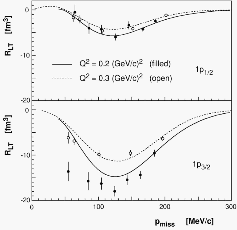
Figure 1: Longitudinal-transverse interference effective responses $R_{LT}$ as a function of $p_{\rm miss}$ for the removal of protons from the $1p$-shell of $\rm{}^{16}O$. The open and filled circles were extracted from QE data obtained by Chinitz et al. at $Q^{2}$ = 0.3 (GeV/$c$)² and Spaltro et al. at $Q^{2}$ = 0.2 (GeV/$c$)², respectively. The dashed ($Q^{2}$ $=$ 0.3 (GeV/$c$)²) and solid ($Q^{2}$ $=$ 0.2 (GeV/$c$)²) curves are modern rdwia calculations. Overall, agreement is good, and improves with increasing $Q^{2}$.

I.2 Higher missing energies

Few data are available for ¹⁶O$(e,e^{\prime}p)$ at higher $E_{\rm miss}$, and much of what is known about this excitation region is from studies of other nuclei such as ¹²C. At MIT-Bates, a series of ¹²C$(e,e^{\prime}p)$ experiments have been performed at missing energies above the two-nucleon emission threshold (see Refs. Lourie et al. (1986); Ulmer et al. (1987); Weinstein et al. (1990); Holtrop et al. (1998); Morrison et al. (1999)). The resulting cross-section data were much larger than the predictions of single-particle knockout models . In particular, Ulmer et al. Ulmer et al. (1987) identified a marked increase in the transverse-longitudinal difference $S_{T}-S_{L}$ . A similar increase has subsequently been observed by Lanen et al. for ⁶Li Lanen et al. (1990), by van der Steenhoven et al. for ¹²C van der Steenhoven et al. (1988), and most recently by Dutta et al. for ¹²C Dutta et al. (2000), ⁵⁶Fe, and ¹⁹⁷Au Dutta . The transverse increase exists over a large range of four-momentum transfers, though the excess at lower $p_{\rm miss}$ seems to decrease with increasing $Q^{2}$. Theoretical attempts by Takaki Takaki (1989), the Ghent Group Ryckebusch et al. (1997), and Gil et al. Gil et al. (1997) to explain the data at high $E_{\rm miss}$ using two-body knockout models coupled to Final-State Interactions (FSI) have not succeeded. Even for QE kinematics, this transverse increase which starts at the two-nucleon knockout threshold seems to be a strong signature of multinucleon currents.

II Experiment

This experiment Saha et al. (1989); Fissum et al. (1997), first proposed by Bertozzi et al. in 1989, was the inaugural physics investigation performed in Hall A hal (the High Resolution Spectrometer Hall) at the Thomas Jefferson National Accelerator Facility (JLab) jla . An overview of the apparatus in the Hall at the time of this measurement is shown in Fig. 2. For a thorough discussion of the experimental infrastructure and its capabilities, the interested reader is directed to the paper by Alcorn et al. Alcorn et al. . For the sake of completeness, a subset of the aforementioned information is presented here.

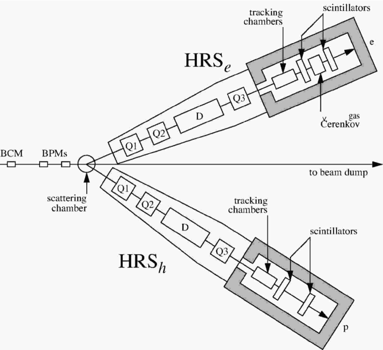
Figure 2: The experimental infrastructure in Hall A at Jefferson Lab at the time of this experiment. The electron beam passed through a beam-current monitor (BCM) and beam-position monitors (BPMs) before striking a waterfall target located in the scattering chamber. Scattered electrons were detected in the HRS_e, while knocked-out protons were detected in the HRS_h. Non-interacting electrons were dumped. The spectrometers could be rotated about the central pivot.

II.1 Electron beam

Unpolarized 70 $\mu$A continuous electron beams with energies of 0.843, 1.643, and 2.442 GeV (corresponding to the virtual photon polarizations shown in Table 1) were used for this experiment. Subsequent analysis of the data demonstrated that the actual beam energies were within 0.3% of the nominal values Gao et al. (1998).

Table 1: The QE, constant $(q,\omega)$ kinematics employed in this measurement. At each beam energy, $q$ $\approx$ 1 GeV/$c$.

$E_{\rm beam}$	$\theta_{e}$	virtual photon	$\theta_{pq}$
(GeV)	(∘)	polarization	(∘)
0.843	100.76	0.21	0, 8, 16
1.643	37.17	0.78	0, $\pm$8
2.442	23.36	0.90	0,$\pm$2.5, $\pm$8, $\pm$16, $\pm$20

The typical laboratory $\pm$4$\sigma$ beam envelope at the target was 0.5 mm (horizontal) by 0.1 mm (vertical). Beam-current monitors bcm (2001) (calibrated using an Unser monitor Unser (1981)) were used to determine the total charge delivered to the target to an accuracy of 2% Ulmer (1998). Beam-position monitors (BPMs) Barry et al. (1990, 1991) were used to ensure the location of the beam at the target was no more than 0.2 mm from the beamline axis, and that the instantaneous angle between the beam and the beamline axis was no larger than 0.15 mrad. The readout from the BCM and BPMs was continuously passed into the data stream epi . Non-interacting electrons were dumped in a well-shielded, high-power beam dump Sinclair (1992) located roughly 30 m from the target.

II.2 Target

A waterfall target Garibaldi et al. (1992) positioned inside a scattering chamber located at the center of the Hall provided the H₂O used for this study of ¹⁶O. The target canister was a rectangular box 20 cm long $\times$ 15 cm wide $\times$ 10 cm high containing air at atmospheric pressure. The beam entrance and exit windows to this canister were respectively 50 $\mu$m and 75 $\mu$m gold-plated beryllium foils. Inside the canister, three thin, parallel, flowing water films served as targets. This three-film configuration was superior to a single film 3$\times$ thicker because it reduced the target-associated multiple scattering and energy loss for particles originating in the first two films and it allowed for the determination of the film in which the scattering vertex was located, thereby facilitating a better overall correction for energy loss. The films were defined by 2 mm $\times$ 2 mm stainless-steel posts. Each film was separated by 25 mm along the direction of the beam, and was rotated beam right such that the normal to the film surface made an angle of 30^∘ with respect to the beam direction. This geometry ensured that particles originating from any given film would not intersect any other film on their way into the spectrometers.

The thickness of the films could be changed by varying the speed of the water flow through the target loop via a pump. The average film thicknesses were fixed at (130 $\pm$ 2.5%) mg/cm² along the direction of the beam throughout the experiment, which provided a good trade-off between resolution and target thickness. The thickness of the central water film was determined by comparing ¹⁶O$(e,e^{\prime})$ cross-section data measured at $q$ $\approx$ 330 MeV/$c$ obtained from both the film and a (155 $\pm$ 1.5%) mg/cm² BeO target foil placed in a solid-target ladder mounted beneath the target canister. The thicknesses of the side films were determined by comparing the concurrently measured ¹H$(e,e)$ cross section obtained from these side films to that obtained from the central film. Instantaneous variations in the target-film thicknesses were monitored throughout the entire experiment by continuously measuring the ¹H$(e,e)$ cross section.

II.3 Spectrometers and detectors

The base apparatus used in the experiment was a pair of optically identical 4 GeV/$c$ superconducting High Resolution Spectrometers (HRS) hrs . These spectrometers have a nominal 9% momentum bite and a FWHM momentum resolution $\Delta p/p$ of roughly 10^-4. The nominal laboratory angular acceptance is $\pm$25 mrad (horizontal) by $\pm$50 mrad (vertical). Scattered electrons were detected in the Electron Spectrometer (HRS_e), and knocked-out protons were detected in the Hadron Spectrometer (HRS_h) (see Fig. 2). Before the experiment, the absolute momentum calibration of the spectrometers was determined to $\Delta p/p$ = 1.5 $\times$ 10^-3 Gao et al. (1998). Before and during the experiment, both the optical properties and acceptances of the spectrometers were studied Liyanage et al. (1998). Some optical parameters are presented in Table 2.

Table 2: Selected results from the optics commissioning.

	resolution	reconstruction
parameter	(FWHM)	accuracy
out-of-plane angle	6.00 mrad	$\pm$0.60 mrad
in-plane angle	2.30 mrad	$\pm$0.23 mrad
$y_{\rm target}$	2.00 mm	$\pm$0.20 mm
$\Delta p/p$	2.5 $\times$ 10-4	-

During the experiment, the locations of the spectrometers were surveyed to an accuracy of 0.3 mrad at every angular location Liang (1998). The status of the magnets was continuously monitored and logged epi .

The detector packages were located in well-shielded detector huts built on decks located above each spectrometer (approximately 25 m from the target and 15 m above the floor of the Hall). The bulk of the instrumentation electronics was also located in these huts, and operated remotely from the Counting House. The HRS_e detector package consisted of a pair of thin scintillator planes tri used to create triggers, a Vertical Drift Chamber (VDC) package Fissum et al. (2001, 2000) used for particle tracking, and a Gas Čerenkov counter Iodice et al. (1998) used to distinguish between $\pi^{-}$ and electron events. Identical elements, except for the Gas Čerenkov counter, were also present in the HRS_h detector package. The status of the various detector subsystems was continuously monitored and logged epi . The individual operating efficiencies of each of these three devices was $>$99%.

II.4 Electronics and data acquisition

For a given spectrometer, a coincidence between signals from the two trigger-scintillator planes indicated a ‘single-arm’ event. Simultaneous HRS_e and HRS_h singles events were recorded as ‘coincidence’ events. The basic trigger logic daq allowed a prescaled fraction of single-arm events to be written to the data stream. Enough HRS_e singles were taken for a 1% statistics ¹H$(e,e)$ cross-section measurement at each kinematics. Each spectrometer had its own VME crate (for scalers) and FASTBUS crate (for ADCs and TDCs). The crates were managed by readout controllers (ROCs). In addition to overseeing the state of the run, a trigger supervisor (TS) generated the triggers which caused the ROCs to read out the crates on an event-by-event basis. The VME (scaler) crate was also read out every ten seconds. An event builder (EB) collected the resulting data shards into events. An analyzer/data distributer (ANA/DD) analyzed and/or sent these events to the disk of the data-acquisition computer. The entire data-acquisition system was managed using the software toolkit CODA cod .

Typical scaler events were about 0.5 kb in length. Typical single-arm events were also about 0.5 kb, while typical coincidence events were about 1.0 kb. The acquisition deadtime was monitored by measuring the TS output-to-input ratio for each event type. The event rates were set by varying the prescale factors and the beam current such that the DAQ computer was busy at most only 20% of the time. This resulted in a relatively low event rate (a few kHz), at which the electronics deadtime was $<$1%. Online analyzers dhi were used to monitor the quality of the data as it was taken. Eventually, the data were transferred to magnetic tape. The ultimate data analysis was performed on the DEC-8400 CPU farm ABACUS aba at the Massachusetts Institute of Technology using the analysis package espace esp .

III Analysis

The interested reader is directed to the Ph.D. theses of Gao Gao (1999) and Liyanage Liyanage (1999) for a complete discussion of the data analysis. For the sake of completeness, a subset of the aforementioned information is presented here.

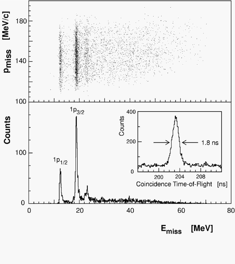
Figure 3: Yield spectrum obtained at $E_{\rm beam}$ = 0.843 GeV and $\theta_{pq}$ = +8^∘, corresponding to $p_{\rm miss}$ $=$ 148 MeV/$c$. Pion rejection has been performed, and all timing corrections have been applied. The top panel shows a scatterplot of $p_{\rm miss}$ versus $E_{\rm miss}$. The dark vertical bands project into the peaks located at 12.1 and 18.3 MeV in the bottom panel. These peaks correspond to protons knocked-out of the 1$p_{1/2}$- and 1$p_{3/2}$-states of ¹⁶O, respectively. The $E_{\rm miss}$ resolution was roughly 0.9 MeV FWHM, which did not allow for separation of the $2s_{1/2}1d_{5/2}$-doublet located at $E_{\rm miss}$ $=$ 17.4 MeV from the $1p_{3/2}$-state at 18.3 MeV. The bump located at roughly 23 MeV is a negative-parity doublet which was not investigated. The insert shows the corresponding optimized coincidence TOF peak which has a FWHM of 1.8 ns. The signal-to-noise ratio was about 8:1 in these kinematics.

III.1 Timing corrections and particle identification

Identification of coincidence $(e,e^{\prime}p)$ events was in general a straightforward process. Software corrections were applied to remove timing variations induced by the trigger-scintillator circuit and thus sharpen all flight-time peaks. These included corrections to proton flight times due to variations in the proton kinetic energies, and corrections for variations in the electron and proton path lengths through the spectrometers. Pion rejection was performed using a flight-time cut for $\pi^{+}$s in the HRS_h and the Gas Čerenkov for $\pi^{-}$s in the HRS_e. A sharp, clear, coincidence Time-of-Flight (TOF) peak with a FWHM of 1.8 ns resulted (see Fig. 3). High-energy correlated protons which punched through the HRS_h collimator ($<$10% of the prompt yield) were rejected by requiring both spectrometers to independently reconstruct the coincidence-event vertex in the vicinity of the same water film. The resulting prompt-peak yields for each water film were corrected for uncorrelated (random) events present in the peak-time region on a bin-by-bin basis as per the method suggested by Owens Owens (1990). These per-film yields were then normalized individually.

III.2 Normalization

The relative focal-plane efficiencies for each of the two spectrometers were measured independently for each of the three water films at every spectrometer excitation used in the experiment. By measuring the same single-arm cross section at different locations on the spectrometer focal planes, variations in the relative efficiencies were identified. The position variation across the focal plane was investigated by systematically shifting the central excitation of the spectrometer about the mean momentum setting in a series of discrete steps such that the full momentum acceptance was ‘mapped’. A smooth, slowly varying dip-region cross section was used instead of a single discrete peak for continuous coverage of the focal plane. The relative-efficiency profiles were unfolded from these data using the program releff Baghaei (1988) by Baghaei. For each water film, solid-angle cuts were then applied to select the flat regions of the angular acceptance. These cuts reduced the spectrometer apertures by roughly 20% to about 4.8 msr. Finally, relative-momentum cuts were applied to select the flat regions of momentum acceptance. These cuts reduced the spectrometer momentum acceptance by roughly 22% to $-$3.7% $<$ $\delta$ $<$ 3.3%. The resulting acceptance profile of each spectrometer was uniform to within 1%.

The absolute efficiency at which the two spectrometers operated in coincidence mode was given by

$$\epsilon=\epsilon_{e}\cdot\epsilon_{p}\cdot\epsilon_{\rm coin},$$ (1)

where $\epsilon_{e}$ was the single-arm HRS_e efficiency, $\epsilon_{p}$ was the single-arm HRS_h efficiency, and $\epsilon_{\rm coin}$ was the coincidence-trigger efficiency. The quantity ($\epsilon_{p}\cdot\epsilon_{\rm coin}$) was measured at $\theta_{pq}$ $=$ 0^∘ at $E_{\rm beam}$ = 0.843 GeV using the ¹H$(e,e)$ reaction. A 0.7 msr collimator was placed in front of the HRS_e. In these kinematics, the cone of recoil protons fit entirely into the central flat-acceptance region of the HRS_h. The number of ¹H$(e,e)$ events where the proton was also detected was compared to the number of ¹H$(e,e)$ events where the proton was not detected to yield a product of efficiencies ($\epsilon_{p}\cdot\epsilon_{\rm coin}$) of 98.9%. The 1.1% effect was due to proton absorption in the waterfall target exit windows, spectrometer windows, and the first layer of trigger scintillators. Since the central field of the HRS_h was held constant throughout the entire experiment, this measurement was applicable to each of the hadron kinematics employed. A similar method was used to determine the quantity ($\epsilon_{e}\cdot\epsilon_{\rm coin}$) at each of the three HRS_e field settings. Instead of a collimator, software cuts applied to the recoil protons were used to ensure that the cone of scattered electrons fit entirely into the central flat-acceptance region of the HRS_e. This product of efficiencies was $>$99%. Thus, the coincidence efficiency $\epsilon_{\rm coin}$ was firmly established at nearly 100%. A nominal systematic uncertainty of $\pm 1.5\%$ was attributed to $\epsilon$.

The quantity ($L\cdot\epsilon_{e}$), where $L$ is the luminosity (the product of the effective target thickness and the number of incident electrons) was determined to $\pm$4% by comparing the measured ¹H$(e,e)$ cross section for each film at each of the electron kinematics to a parametrization established at a similar $Q^{2}$ by Simon et al. Simon et al. (1980) and Price et al. Price et al. (1971) (see Fig. 4). The results reported in this paper have all been normalized in this fashion. As a consistency check, a direct absolute calculation of ($L\cdot\epsilon_{e}$) using information from the BCMs, the calibrated thicknesses of the water films, and the single-arm HRS_e efficiency agrees within uncertainty.

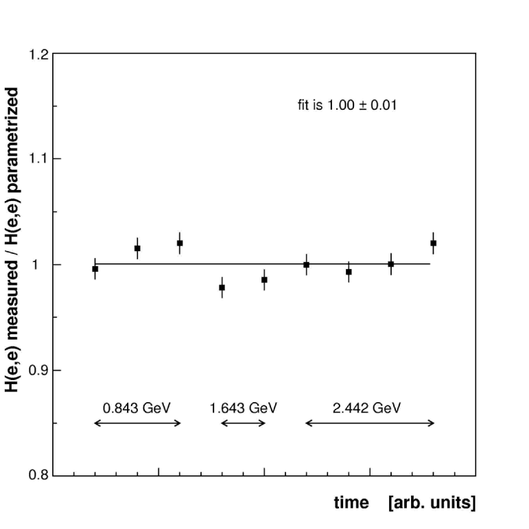
Figure 4: Measured ¹H$(e,e)$ cross-section data normalized to the absolute predictions of a parametrization at similiar $Q^{2}$. Statistical error bars are shown. The data shown were taken over the course of a three-month run period. The different data points for each $E_{\rm beam}$ represent different HRS_h angular settings.

At every kinematics, a Monte Carlo of the phase-space volume subtended by each experimental bin was performed. For each water foil, $N_{0}$ software $(e,e^{\prime}p)$ events were generated, uniformly distributed over the scattered-electron and knocked-out proton momenta ($p_{e}$, $p_{p}$) and in-plane and out-of-plane angles ($\phi_{e}$, $\theta_{e}$, $\phi_{p}$, $\theta_{p}$). For each of these events, all of the kinematic quantities were calculated. The flat-acceptance cuts determined in the analysis of the relative focal-plane efficiency data were then applied, as were all other cuts that had been performed on the actual data. The pristine detection volume $\Delta V_{b}$($E_{\rm miss}$, $p_{\rm miss}$, $\omega$, $Q^{2}$) subtended by a bin $b$($\Delta E_{\rm miss}$, $\Delta p_{\rm miss}$, $\Delta\omega$, $\Delta Q^{2}$) containing $N_{b}$ pseudoevents was thus

$$\Delta V_{b}(E_{\rm miss},p_{\rm miss},\omega,Q^{2})=$$ (2)

$$\frac{N_{b}}{N_{0}}~{}[(\Delta p_{e}\cdot\Delta\Omega_{e})\cdot(\Delta p_{p}\cdot\Delta\Omega_{p})]\;,$$

where the quantity $(\Delta p_{e}\cdot\Delta\Omega_{e})\cdot(\Delta p_{p}\cdot\Delta\Omega_{p})$ was the total volume sampled over in the Monte Carlo (purposely set larger than the experimental acceptance in all dimensions ). The pseudodata were binned exactly as the real data, and uniformly on both sides of $\bm{q}$. At each kinematics, the bin with the largest volume $\Delta V_{\rm max}$ was located. Only bins subtending volumes larger than 50% of $\Delta V_{\rm max}$ were analyzed further.

Corrections based on the TS output-to-input ratio were applied to the data to account for the acquisition deadtime to coincidence events. On average, these corrections were roughly 20%. An acquisition Monte Carlo by Liang lia was used to cross-check these corrections and establish the absolute uncertainty in them at 2%.

Corrections to the per-film cross-section data for electron radiation before and after scattering were calculated on a bin-by-bin basis in two ways: first using a version of the code radcor by Quint Quint (1998) modified by Florizone Florizone (1999), and independently, the prescriptions of Borie and Dreschel Borie and Drechsel (1971) modified by Templon et al. Templon et al. (2000) for use within the simulation package mceep written by Ulmer mce . The two approaches agreed to within the statistical uncertainty of the data and amounted to $<$55% of the measured cross section for the bound states, and $<$15% of the measured cross section for the continuum. Corrections for proton radiation at these energies are much less than 1% and were not performed.

III.3 Cross section

The radiatively corrected average cross section in the bin $b$($\Delta E_{\rm miss}$, $\Delta p_{\rm miss}$, $\Delta\omega$, $\Delta Q^{2}$) was calculated according to

$$\left<\frac{d^{6}\sigma}{d\omega~{}d\Omega_{e}~{}dE_{\rm miss}~{}d\Omega_{p}}\right>_{b}=$$ (3)

$$\frac{R_{{}^{16}{\rm O}(e,e^{\prime}p)}}{(L\cdot\epsilon_{e})(\epsilon_{p}\cdot\epsilon_{\rm coin})}\left(\frac{Y_{b}}{\Delta V_{b}}\right),$$

where $Y_{b}$ was the total number of real events which were detected in $b$($\Delta E_{\rm miss}$, $\Delta p_{\rm miss}$, $\Delta\omega$, $\Delta Q^{2}$), ${\Delta V_{b}}$ was the phase-space volume, and $R_{{}^{16}{\rm O}(e,e^{\prime}p)}$ was a correction applied to account for events which radiated in or out of $\Delta V_{b}$. The average cross section was calculated as a function of $E_{\rm miss}$ for a given kinematic setting . Bound-state cross-section data for the $1p$-shell were extracted by integrating over the appropriate range in $E_{\rm miss}$, weighting with the appropriate Jacobian . Five-fold differential cross-section data for QE proton knockout from the $1p$-shell of ¹⁶O are presented in Tables LABEL:table:pshellpararesults and LABEL:table:pshellperpresults. Six-fold differential cross-section data for QE proton knockout from ¹⁶O at higher $E_{\rm miss}$ are presented in Tables LABEL:table:0843cont000deg $-$ LABEL:table:2442cont020deg.

III.4 Asymmetries and response functions

In the One-Photon Exchange Approximation, the unpolarized six-fold differential cross section may be expressed in terms of four independent response functions as (see Refs. Picklesimer and Van Orden (1989); Raskin and Donnelly (1989); Kelly (1996))

$$\frac{d^{6}\sigma}{d\omega~{}d\Omega_{e}~{}dE_{\rm miss}~{}d\Omega_{p}}=K~{}\sigma_{\rm Mott}\left[v_{L}R_{L}+v_{T}R_{T}+v_{LT}R_{LT}\cos(\phi)+v_{TT}R_{TT}\cos(2\phi)\right],$$ (4)

where $K$ is a phase-space factor, $\sigma_{\rm Mott}$ is the Mott cross section, and the $v_{\rm i}$ are dimensionless kinematic factors . Ideal response functions are not directly measureable because electron distortion does not permit the azimuthal dependences to be separated exactly. The effective response functions which are extracted by applying Eq. (4) to the data are denoted $R_{L}$ (longitudinal), $R_{T}$ (transverse), $R_{LT}$ (longitudinal-transverse), and $R_{TT}$ (transverse-transverse). They contain all the information which may be extracted from the hadronic system using $(e,e^{\prime}p)$. Note that the $v_{\rm i}$ depend only on ($\omega$, $Q^{2}$, $\theta_{e}$), while the response functions depend on ($\omega$, $Q^{2}$, $E_{\rm miss}$, $p_{\rm miss}$).

The individual contributions of the effective response functions may be separated by performing a series of cross-section measurements varying $v_{\rm i}$ and/or $\phi$, but keeping $q$ and $\omega$ constant . In the case where the proton is knocked-out of the nucleus in a direction parallel to $\bm{q}$ (‘parallel’ kinematics), the interference terms $R_{LT}$ and $R_{TT}$ vanish, and a Rosenbluth separation Rosenbluth (1950) may be performed to separate $R_{L}$ and $R_{T}$. In the case where the proton is knocked-out of the nucleus in the scattering plane with a finite angle $\theta_{pq}$ with respect to $\bm{q}$ (‘quasiperpendicular’ kinematics), the asymmetry $A_{LT}$ and the interference $R_{LT}$ may be separated by performing symmetric cross-section measurements on either side of $\bm{q}$ ($\phi$ $=$ 0^∘ and $\phi$ $=$ 180^∘). The contribution of $R_{TT}$ cannot be separated from that of $R_{L}$ with only in-plane measurements; however, by combining the two techniques, an interesting combination of response functions $R_{T}$, $R_{LT}$, and $R_{L+TT}$ may be extracted.

For these data, effective response-function separations were performed where the phase-space overlap between kinematics permitted. For these separations, bins were selected only if their phase-space volumes $\Delta V_{b}$ were all simultaneously 50% of $\Delta V_{\rm max}$. Separated effective response functions for QE proton knockout from the $1p$-shell of ¹⁶O are presented in Tables LABEL:table:pshellrlrt, LABEL:table:pshellrlttrt, and LABEL:table:pshellaltrlt. Separated effective response functions for QE proton knockout from the ¹⁶O continuum are presented in Tables LABEL:table:contrlrt, LABEL:table:contrlttrt, and LABEL:table:contrlt.

III.5 Systematic uncertainties

The systematic uncertainties in the cross-section measurements were classified into two categories – kinematic-dependent uncertainties and scale uncertainties. For a complete discussion of how these uncertainties were evaluated, the interested reader is directed to a report by Fissum and Ulmer Fissum and Ulmer (2002). For the sake of completeness, a subset of the aforementioned information is presented here.

In a series of simulations performed after the experiment, mceep was used to investigate the intrinsic behavior of the cross-section data when constituent kinematic parameters were varied over the appropriate experimentally determined ranges presented in Table 3. Based on the experimental data, the high-$E_{\rm miss}$ region was modelled as the superposition of a peak-like $1s_{1/2}$-state on a flat continuum. Contributions to the systematic uncertainty from this flat continuum were taken to be small, leaving only those from the $1s_{1/2}$-state. The ¹⁶O$(e,e^{\prime}p)$ simulations incorporated as physics input the bound-nucleon rdwia calculations detailed in Section IV.1, which were based on the experimental $1p$-shell data.

Table 3: Kinematic-dependent systematic uncertainties folded into the mceep simulation series.

Quantity	description	$\delta$
$E_{\rm beam}$	beam energy	1.6 $\times$ 10-3
$\phi_{\rm beam}$	in-plane beam angle	ignored
$\theta_{\rm beam}$	out-of-plane beam angle	2.0 mrad
$p_{e}$	scattered electron momentum	1.5 $\times$ 10-3
$\phi_{e}$	in-plane scattered electron angle	0.3 mrad
$\theta_{e}$	out-of-plane scattered electron angle	2.0 mrad
$p_{p}$	proton momentum	1.5 $\times$ 10-3
$\phi_{p}$	in-plane proton angle	0.3 mrad
$\theta_{p}$	out-of-plane proton angle	2.0 mrad

For each kinematics, the central water foil was considered, and 1M events were generated. In evaluating the simulation results, the exact cuts applied in the actual data analyses were applied to the pseudo-data, and the cross section was evaluated for the identical $p_{\rm miss}$ bins used to present the results. The experimental constraints to the kinematic-dependent observables afforded by the overdetermined ¹H$(e,ep)$ reaction were exploited to calibrate and constrain the experimental setup. The in-plane electron and proton angles $\phi_{e}$ and $\phi_{p}$ were chosen as independent parameters. When a known shift in $\phi_{e}$ was made, $\phi_{p}$ was held constant and the complementary variables $E_{\rm beam}$, $p_{e}$, and $p_{p}$ were varied as required by the constraints enforced by the ¹H$(e,ep)$ reaction. Similarly, when a known shift in $\phi_{p}$ was made, $\phi_{e}$ was held constant and the complementary variables $E_{\rm beam}$, $p_{e}$, and $p_{p}$ were varied as appropriate. The overall constrained uncertainty was taken to be the quadratic sum of the two contributions.

The global convergence of the uncertainty estimate was examined for certain extreme kinematics, where 10M-event simulations (which demonstrated the same behavior) were performed. The behavior of the uncertainty as a function of $p_{\rm miss}$ was also investigated by examining the uncertainty in the momentum bins adjacent to the reported momentum bin in exactly the same fashion. The kinematically induced systematic uncertainty in the ¹⁶O$(e,e^{\prime}p)$ cross-section data was determined to be dependent upon $p_{\rm miss}$, with an average value of 1.4%. The corresponding uncertainties in the ¹H$(e,e)$ cross-section data were determined to be negligible.

The scale systematic uncertainties which affect each of the cross-section measurements are presented in Table 4. As previously mentioned, the ¹⁶O$(e,e^{\prime}p)$ cross-section results reported in this paper have been normalized by comparing simultaneously measured ¹H$(e,e)$ cross-section data to a parametrization established at a similar $Q^{2}$. Thus, the first seven listed uncertainties simply divide out of the quotient, such that only the subsequent uncertainties affect the results. The average systematic uncertainty associated with a $1p$-shell cross section was 5.6%, while that for the continuum was 5.9%. The small difference was due to contamination of the high-$E_{\rm miss}$ data by collimator punch-through events.

Table 4: Summary of the scale systematic uncertainties contributing to the cross-section data. The first seven entries do not contribute to the systematic uncertainties in the reported cross-section data as they contribute equally to the ¹H$(e,e)$ cross-section data to which the ¹⁶O$(e,e^{\prime}p)$ are normalized.

Quantity	description	$\delta$ (%)
$\eta_{\rm DAQ}$	data acquisition deadtime correction	2.0
$\eta_{\rm elec}$	electronics deadtime correction	$<$1.0
$\rho t^{\prime}$	effective target thickness	2.5
$N_{e}$	number of incident electrons	2.0
$\epsilon_{e}$	electron detection efficiency	1.0
$\Delta\Omega_{e}$	HRSe solid angle	2.0
$\epsilon_{e}\cdot\epsilon_{p}\cdot\epsilon_{\rm coin}$	product of electron, proton, and coincidence efficiencies	1.5
$L\cdot\epsilon_{e}$	obtained from a form-factor parametrization of ${}^{1}{\rm H}(e,e)$	4.0
$R_{{}^{16}{\rm O}(e,e^{\prime}p)}$	radiative correction to the ${}^{16}{\rm O}(e,e^{\prime}p)$ data	2.0
$R_{{}^{1}{\rm H}(e,e)}$	radiative correction to the ${}^{1}{\rm H}(e,e)$ data	2.0
$\epsilon_{p}\cdot\epsilon_{\rm coin}$	product of proton and coincidence efficiencies	$<$1.0
$\Delta\Omega_{p}$	HRSh solid angle	2.0
punchthrough	protons which punched through the HRSh collimator	2.0

The quality of these data in terms of their associated systematic uncertainties was clearly demonstrated by the results obtained for the effective response-function separations. In Fig. 5, cross-section data for the $1p$-shell measured in parallel kinematics at three different beam energies are shown as a function of the separation lever arm $v_{T}/v_{L}$. The values of the effective response functions $R_{L}$ (offset) and $R_{T}$ (slope) were extracted from the fitted line. The extremely linear trend in the data indicated that the magnitude of the systematic uncertainties was small, and that statistical uncertainties dominated. This is not simply a test of the One-Photon Exchange Approximation employed in the data analysis as it has been demonstrated by Traini et al. Traini et al. (1988) and Udías Udías that the linear behavior of the Rosenbluth plot persists even after Coulomb distortion is included.

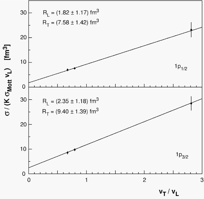
Figure 5: Cross-section data for the removal of protons from the 1$p$-shell of ¹⁶O measured in parallel kinematics at three different beam energies as a function of the separation lever arm $v_{T}/v_{L}$. The data points correspond to beam energies of 2.442, 1.643, and 0.843 GeV from left to right. The effective response functions $R_{L}$ (offset) and $R_{T}$ (slope) have been extracted from the fitted line. The uncertainties shown are statistical only. The extremely linear behavior of the data (which persists even after corrections for Coulomb distortion are applied) indicates that the statistical uncertainties were dominant (see Section III.5 for a complete discussion).

Given the applicability of the One-Photon Exchange Approximation at these energies, the quality of the data was also demonstrated by the results extracted from identical measurements which were performed in different electron kinematics. The asymmetries $A_{LT}$ and effective response functions $R_{LT}$ for QE proton knockout were extracted for both $E_{\rm beam}$ $=$ 1.643 GeV and 2.442 GeV for $\theta_{pq}$ $=$ $\pm 8^{\circ}$ ($p_{\rm miss}$ $=$ 148 MeV/$c$). They agree within the statistical uncertainty. Table LABEL:table:pshellaltrlt presents the results at both beam energies for $1p$-shell knockout for $<Q^{2}>$ $=$ 0.800 (GeV/$c$)², $<\omega>$ $=$ 436 MeV, and $<T_{p}>$ $=$ 427 MeV, while Fig. 6 shows the results for 25 $<$ $E_{\rm miss}$ $<$ 60 MeV.

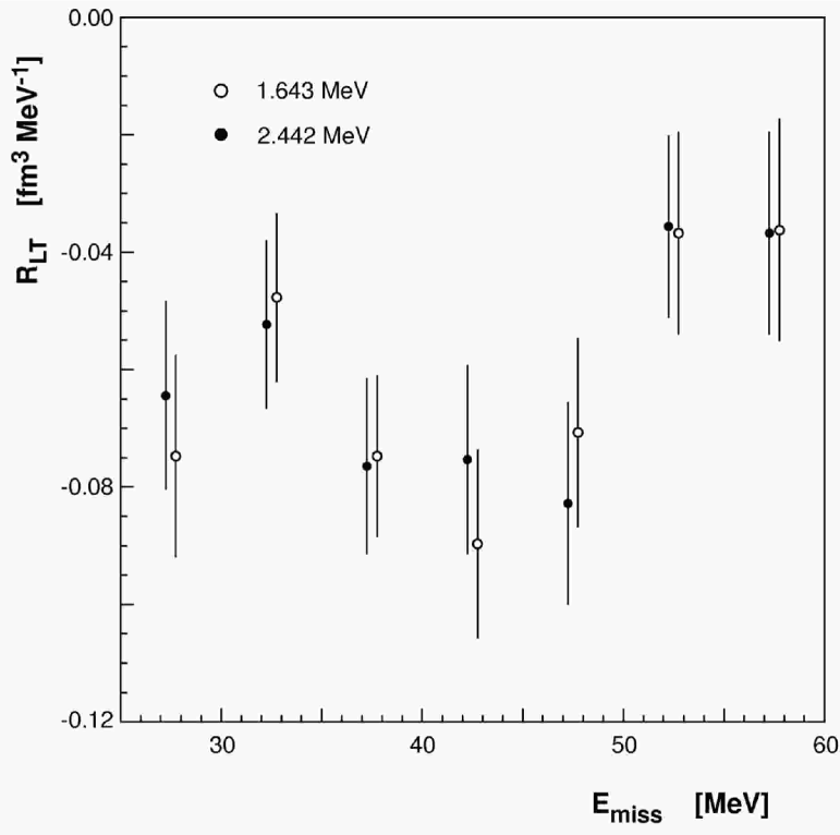
Figure 6: $R_{LT}$ for $\theta_{pq}$ $=$ $\pm 8^{\circ}$ ($p_{\rm miss}$ $=$ 145 MeV/$c$) as a function of $E_{\rm miss}$ for $E_{\rm beam}$ $=$ 1.643 GeV and 2.442 GeV. Statistical uncertainties only are shown. The statistical agreement over a broad range of $E_{\rm miss}$ emphasizes the systematic precision of the measurement (see Section III.5 for a complete discussion). Note that the averages of these $R_{LT}$ values are presented as the $p_{\rm miss}$ $=$ 145 MeV/$c$ data in Fig. 22 and Table LABEL:table:contrlt.

IV Theoretical Overview

In the following subsections, overviews of Relativistic Distorted-Wave Impulse Approximation (rdwia), Relativistic Optical-Model Eikonal Approximation (romea), and Relativistic Multiple-Scattering Glauber Approximation (rmsga) calculations are presented.

IV.1 RDWIA

Reviews of work on proton electromagnetic knockout using essentially nonrelativistic approaches may be found in Refs. Frullani and Mougey (1984); Kelly (1996); Boffi et al. (1996). As previously mentioned, the Relativistic Distorted-Wave Impulse Approximation (rdwia) was pioneered by Picklesimer, Van Orden, and Wallace Picklesimer et al. (1985); Picklesimer and Van Orden (1987, 1989) and subsequently developed in more detail by several groups (see Refs. McDermott (1990); Jin et al. (1992); Udías et al. (1993); Hedayati-Poor et al. (1995); Kelly (1999a); Udías and Vignote (2000); Meucci et al. (2001)). In Section IV.1.1, the rdwia formalism for direct knockout based upon a single-nucleon operator is outlined in sufficient detail that the most important differences with respect to nonrelativistic dwia may be identified. In Section IV.1.2, a direct numerical comparison between two different implementations of rdwia is presented.

IV.1.1 Formalism

The five-fold differential cross section for the exclusive $A(e,e^{\prime}N)B$ reaction leading to a discrete final state takes the form (see Ref. Kelly (1996))

$$\frac{d^{5}\sigma}{d\varepsilon_{f}d\Omega_{e}d\Omega_{N}}=K\frac{\varepsilon_{f}}{\varepsilon_{i}}\frac{\alpha^{2}}{Q^{4}}\eta_{\mu\nu}{\cal W}^{\mu\nu}~{},$$ (5)

where

$$K={\cal R}\frac{p_{N}E_{N}}{(2\pi)^{3}}$$ (6)

is a phase-space factor, $k_{i}=(\varepsilon_{i},{\bm{k}}_{i})$ and $k_{f}=(\varepsilon_{f},{\bm{k}}_{f})$ are the initial and final electron momenta, $p_{A}=(E_{A},{\bm{p}}_{A})$ and $p_{B}=(E_{B},{\bm{p}}_{B})$ are the initial and final target momenta, $p_{N}=(E_{N},{\bm{p}}_{N})$ is the ejected-nucleon momentum, ${q}={k}_{i}-{k}_{f}=(\omega,{\bm{q}}\hskip 1.42262pt)$ is the momentum transfer carried by the virtual photon, $Q^{2}=-q_{\mu}q^{\mu}={\bm{q}}\hskip 1.42262pt^{2}-\omega^{2}$ is the photon virtuality, and

$${\cal R}=\left|1-\frac{{\bm{v}}_{N}\cdot{\bm{v}}_{B}}{{\bm{v}}_{N}\cdot{\bm{v}}_{N}}\right|^{-1}$$ (7)

(with $v_{N}=p_{N}/E_{N}$) is a recoil factor which adjusts the nuclear phase space for the missing-energy constraint. In the One-Photon Exchange Approximation, the invariant electroexcitation matrix element is represented by the contraction of electron and nuclear response tensors of the form

$$\eta_{\mu\nu} = \langle j_{\mu}j_{\nu}^{\dagger}\rangle$$ (8)

$${\cal W}_{\mu\nu} = \langle{\cal J}_{\mu}{\cal J}_{\nu}^{\dagger}\rangle~{},$$ (9)

where $j^{\mu}$ is the electron current, ${\cal J}^{\mu}$ is a matrix element of the nuclear electromagnetic current, and the angled brackets denote averages over initial states and sums over final states.

The reduced cross section is given by

$$\sigma_{\rm red}=\frac{d^{5}\sigma}{d\varepsilon_{f}d\Omega_{e}d\Omega_{N}}/K\sigma_{eN}~{},$$ (10)

where

$$\sigma_{eN}=\frac{\varepsilon_{f}}{\varepsilon_{i}}\frac{\alpha^{2}}{Q^{4}}\left(\eta_{\mu\nu}{\cal W}^{\mu\nu}\right)_{\rm PWIA}$$ (11)

is the elementary cross section for electron scattering from a moving free nucleon in the Plane-Wave Impulse Approximation (pwia). The pwia response tensor is computed for a free nucleon in the final state, and is given by

$$W^{\mu\nu}_{\rm PWIA}=\frac{1}{2}{\rm Trace}{J^{\mu}{J^{\nu}}^{\dagger}}~{},$$ (12)

where

$$J^{\mu}_{s_{f},s_{i}}=\sqrt{\frac{m^{2}}{\varepsilon_{i}\varepsilon_{f}}}\bar{u}({{\bm{p}}}_{f},s_{f})\Gamma^{\mu}u({{\bm{p}}}_{i},s_{i})$$ (13)

is the single-nucleon current between free spinors normalized to unit flux. The initial momentum (${{\bm{p}}}_{i}={{\bm{p}}}_{f}-{{\bm{q}}}_{\rm eff}$) is obtained from the final ejectile momentum (${\bm{p}}_{f}$) and the effective momentum transfer (${\bm{q}}_{\rm eff}$) in the laboratory frame, and the initial energy is placed on shell. The effective momentum transfer accounts for electron acceleration in the nuclear Coulomb field and is discussed further later in this Section.

In the nonrelativistic pwia limit, $\sigma_{\rm red}$ reduces to the bound-nucleon momentum distribution, and the cross section given in Eq. (5) may be expressed as the product of the phase-space factor $K$, the elementary cross section $\sigma_{eN}$, and the momentum distribution. This is usually referred to ‘factorization’. Factorization is not strictly valid relativistically because the binding potential alters the relationship between lower and upper components of a Dirac wave function – see Ref. Caballero et al. (1998b).

In this Section, it is assumed that the nuclear current is represented by a one-body operator, such that

$${\cal J}^{\mu}=\int d^{3}r\;\exp{(i\bm{t}}\cdot{\bm{r}})\langle\bar{\Psi}^{(-)}({\bm{p}},{\bm{r}}\hskip 1.42262pt)|\Gamma^{\mu}|\phi({\bm{r}}\hskip 1.42262pt)\rangle~{},$$ (14)

where $\phi$ is the nuclear overlap for single-nucleon knockout (often described as the bound-nucleon wave function), $\bar{\Psi}^{(-)}$ is the Dirac adjoint of the time-reversed distorted wave, ${\bm{p}}$ is the relative momentum, and

$$\bm{t}=\frac{E_{B}}{W}{\bm{q}}$$ (15)

is the recoil-corrected momentum transfer in the barycentric frame. Here $(\omega,{\bm{q}}\hskip 1.42262pt)$ and $E_{B}$ are the momentum transfer and the total energy of the residual nucleus in the laboratory frame respectively, and $W=\sqrt{(m_{A}+\omega)^{2}-{\bm{q}}\hskip 1.42262pt^{2}}$ is the invariant mass.

De Forest de Forest Jr. (1983) and Chinn and Picklesimer Chinn and Picklesimer (1992) have demonstrated that the electromagnetic vertex function for a free nucleon can be represented by any of three Gordon-equivalent operators

$$\Gamma_{1}^{\mu}(\bm{p}_{f},\bm{p}_{i}) = \gamma^{\mu}G_{M}(Q^{2})-\frac{P^{\mu}}{2m}F_{2}(Q^{2})$$ (16a)

$$\Gamma_{2}^{\mu}(\bm{p}_{f},\bm{p}_{i}) = \gamma^{\mu}F_{1}(Q^{2})+i\sigma^{\mu\nu}\frac{q_{\nu}}{2m}F_{2}(Q^{2})$$ (16b)

$$\Gamma_{3}^{\mu}(\bm{p}_{f},\bm{p}_{i}) = \frac{P^{\mu}}{2m}F_{1}(Q^{2})+i\sigma^{\mu\nu}\frac{q_{\nu}}{2m}G_{M}(Q^{2})$$ (16c)

where $P=(E_{f}+E_{i},{\bm{p}_{f}}+{\bm{p}_{i}}\hskip 1.42262pt)$. Note the correspondence with Eq. (17) below. Although $\Gamma_{2}$ is arguably the most fundamental because it is defined in terms of the Dirac and Pauli form factors $F_{1}$ and $F_{2}$, $\Gamma_{1}$ is often used because the matrix elements are easier to evaluate. $\Gamma_{3}$ is rarely used but no less fundamental. In all calculations presented here, the momenta in the vertex functions are evaluated using asymptotic laboratory kinematics instead of differential operators.

Unfortunately, as bound nucleons are not on shell, an off-shell extrapolation (for which no rigorous justification exists) is required. The de Forest prescription is employed, in which the energies of both the initial and the final nucleons are placed on shell based upon effective momenta, and the energy transfer is replaced by the difference between on-shell nucleon energies in the operator. Note that the form factors are still evaluated at the $Q^{2}$ determined from the electron-scattering kinematics. In this manner, three prescriptions

$$\bar{\Gamma}_{1}^{\mu} = \gamma^{\mu}G_{M}(Q^{2})-\frac{\bar{P}^{\mu}}{2m}F_{2}(Q^{2})$$ (17a)

$$\bar{\Gamma}_{2}^{\mu} = \gamma^{\mu}F_{1}(Q^{2})+i\sigma^{\mu\nu}\frac{\bar{q}_{\nu}}{2m}F_{2}(Q^{2})$$ (17b)

$$\bar{\Gamma}_{3}^{\mu} = \frac{\bar{P}^{\mu}}{2m}F_{1}(Q^{2})+i\sigma^{\mu\nu}\frac{\bar{q}_{\nu}}{2m}G_{M}(Q^{2})~{},$$ (17c)

are obtained, where

$$\bar{q} = (E_{f}-\bar{E}_{i},{\bm{q}}\hskip 1.42262pt)~{},$$

$$\bar{P} = (E_{f}+\bar{E}_{i},2{\bm{p}_{f}}-{\bm{q}}\hskip 1.42262pt)~{},$$

and where $\bar{E}_{i}=\sqrt{m_{N}^{2}+({\bm{p}_{f}}-{\bm{q}}\hskip 1.42262pt)^{2}}$ is placed on shell based upon the externally observable momenta ${\bm{p}_{f}}$ and ${\bm{q}}$ evaluated in the laboratory frame. When electron distortion is included, the local momentum transfer ${\bm{q}}\rightarrow{\bm{q}}_{\rm eff}$ is interpreted as the effective momentum transfer with Coulomb distortion. These operators are commonly named cc1, cc2, and cc3, and are no longer equivalent when the nucleons are off-shell. Furthermore, the effects of possible density dependence in the nucleon form factors can be evaluated by applying the Local Density Approximation (LDA) to Eq. (17) – see Refs. Chinn and Picklesimer (1992); Kelly (1999a).

The overlap function is represented as a Dirac spinor of the form

$$\phi_{\kappa m}({\bm{r}})=\left(\begin{array}[]{r}f_{\kappa}(r){\cal Y}_{\kappa m}(\hat{r})\\ ig_{-\kappa}(r){\cal Y}_{-\kappa m}(\hat{r})\end{array}\right)~{},$$ (18)

where

$${\cal Y}_{\kappa m}(\hat{r})=\sum_{\nu,m_{s}}\left<\ell\;\;\nu\;\;\frac{1}{2}\;\;m_{s}\mid j\;\;m\;\right>Y_{\ell\nu}(\hat{r})\chi_{m_{s}}$$ (19)

is the spin spherical harmonic and where the orbital and total angular momenta are respectively given by

$$\ell = S_{\kappa}(\kappa+\frac{1}{2})-\frac{1}{2}$$ (20a)

$$j = S_{\kappa}\kappa-\frac{1}{2}~{},$$ (20b)

with $S_{\kappa}={\rm sign}{(\kappa)}$. The functions $f_{\kappa}$ and $g_{\kappa}$ satisfy the usual coupled linear differential equations – see for example Ref. Rose (1961). The corresponding momentum wave function

$$\tilde{\phi}_{\kappa m}({\bm{p}_{m}}\hskip 1.42262pt)=\int d^{3}r\;\exp{(-i{\bm{p}_{m}}\cdot{\bm{r}}\hskip 1.42262pt)}\phi_{\kappa m}({\bm{r}}\hskip 1.42262pt)$$ (21)

then takes the form

$$\tilde{\phi}_{\kappa m}({\bm{p}_{m}}\hskip 1.42262pt)=4\pi i^{-\ell}\left(\begin{array}[]{r}\tilde{f}_{\kappa}(p_{m}){\cal Y}_{\kappa m}(\hat{p}_{m})\\ -S_{\kappa}\tilde{g}_{-\kappa}(p_{m}){\cal Y}_{-\kappa m}(\hat{p}_{m})\end{array}\right)~{},$$ (22)

where

$$\tilde{f}_{\kappa}(p_{m}) = \int dr\;r^{2}j_{\ell}(p_{m}r)f_{\kappa}(r)$$ (23a)

$$\tilde{g}_{-\kappa}(p_{m}) = \int dr\;r^{2}j_{\ell^{\prime}}(p_{m}r)g_{-\kappa}(r)~{},$$ (23b)

and where in the pwia, the initial momentum $\bm{p}_{m}$ would equal the experimental missing momentum $\bm{p}_{\rm miss}$. Thus, the momentum distribution

$$\rho(p_{m})=\frac{1}{2\pi^{2}}\left(|\tilde{f}_{\kappa}(p_{m})|^{2}+|\tilde{g}_{\kappa}(p_{m})|^{2}\right)$$ (24)

is obtained, normalized to

$$4\pi\int dp\;p_{m}^{2}\rho(p_{m})=1$$ (25)

for unit occupancy.

Similarly, let

$$\Psi^{(+)}({\bm{p}},{\bm{r}})=\sqrt{\frac{E+m}{2E}}\left(\begin{array}[]{r}\psi({\bm{r}})\\ \zeta({\bm{r}})\end{array}\right)$$ (26)

represent a wave function of the $N+B$ system with an incoming Coulomb wave and outgoing spherical waves open in all channels. Specific details regarding the boundary conditions may be found in Refs. Satchler (1983); Rawitscher (1997); Kelly (1999b).

The Madrid rdwia calculations Udías et al. (1993) employ a partial-wave expansion of the first-order Dirac equation, leading to a pair of coupled first-order differential equations. Alternatively, the LEA code Kelly by Kelly uses the Numerov algorithm to solve a single second-order differential equation that emerges from an equivalent Schrödinger equation of the form

$$\left[\nabla^{2}+k^{2}-2\mu\left(U^{C}+U^{LS}\bm{L}\cdot\bm{\sigma}\right)\right]\xi=0~{},$$ (27)

where $k$ is the relativistic wave number, $\mu$ is the reduced energy, and

$$U^{C} = \frac{E}{\mu}\left[V+\frac{m}{E}S+\frac{S^{2}-V^{2}}{2E}\right]+U^{D}$$ (28a)

$$U^{D} = \frac{1}{2\mu}\left[-\frac{1}{2r^{2}D}\frac{d}{dr}(r^{2}D^{\prime})+\frac{3}{4}\left(\frac{D^{\prime}}{D}\right)^{2}\right]$$ (28b)

$$U^{LS} = -\frac{1}{2\mu}\frac{D^{\prime}}{rD}$$ (28c)

$$D = 1+\frac{S-V}{E+m}\;.$$ (28d)

$S$ and $V$ are respectively the scalar and vector potential terms of the original four-component Dirac equation (see Ref Kelly (1996)). $D(r)$ is known as the Darwin nonlocality factor and $U^{C}$ and $U^{LS}$ are the central and spin-orbit potentials. The Darwin potential $U^{D}$ is generally quite small. The upper and lower components of the Dirac wave function are then obtained using

$$\psi = D^{1/2}\xi$$ (29a)

$$\zeta = \frac{\bm{\sigma}\cdot{\bm{p}}\hskip 1.42262pt~{}\psi}{E+m+S-V}\;.$$ (29b)

This method is known as direct Pauli reduction Udías et al. (1995); Hedayati-Poor et al. (1995). A very similar approach is also employed by Meucci et al. Meucci et al. (2001). A somewhat similar approach based on the Eikonal Approximation (see the discussion of the romea calculations in Section IV.2) has been employed by Radici et al. Radici et al. (2002, 2003).

For our purposes, the two most important differences between relativistic and nonrelativistic dwia calculations are the suppression of the interior wave function by the Darwin factor in Eq. (29a), and the dynamical enhancement of the lower components of the Dirac spinor (also known as ‘spinor distortion’) by the strong Dirac scalar and vector potentials in Eq. (29b).

As demonstrated in Refs. Boffi et al. (1987); Jin and Onley (1994); Udías et al. (1995), the Darwin factor tends to increase the normalization factors deduced using an rdwia analysis. Distortion of the bound-nucleon spinor destroys factorization and at large $p_{\rm miss}$ produces important oscillatory signatures in the interference response functions, $A_{LT}$, and recoil polarization – see Refs. Caballero et al. (1998a); Kelly (1999b); Udías et al. (1999); Udías and Vignote (2000); Martínez et al. (2002). The effect of spinor distortion within the Effective Momentum Approximation (EMA) has been studied by Kelly Kelly (1999b). The LEA code has subsequently been upgraded to evaluate Eq. (29) without applying the EMA. These two methods for constructing the ejectile distorted waves should be equivalent. The predictions of the LEA and the Madrid codes given identical input are compared in Section IV.1.2.

The approximations made by dwia violate current conservation and introduce gauge ambiguities. The most common prescriptions

$${\cal J}_{q} \rightarrow \frac{\omega}{q}{\cal J}_{0}$$ (30a)

$${\cal J}_{\mu} \rightarrow {\cal J}_{\mu}+\frac{{\cal J}\cdot q}{Q^{2}}q_{\mu}$$ (30b)

$${\cal J}_{0} \rightarrow \frac{q}{\omega}{\cal J}_{q}$$ (30c)

correspond to Coulomb, Landau, and Weyl gauges, respectively. Typically, Gordon ambiguities and sensitivity to details of the off-shell extrapolation are largest in the Weyl gauge. Although there is no fundamental preference for any of these prescriptions, it appears that the data are in general least supportive of the Weyl gauge. Further, the cc1 operator is the most sensitive to spinor distortion while the cc3 operator is the least. The intermediate cc2 is chosen most often for rdwia.

Besides the interaction in the final state of the outgoing proton, in any realistic calculation with finite nuclei, the effect of the distortion of the electron wave function must be taken into account. For relatively light nuclei and large kinetic energies, the EMA for electron distortion (the $q_{\rm eff}$ Approximation) is sufficient – see Refs. Schiff (1956); Giusti and Pacati (1987). In this approach, the electron current is approximated by

$$j^{\mu}(\bm{q}_{\rm eff})\approx\frac{\bar{k}_{i}\bar{k}_{f}}{k_{i}k_{f}}\bar{u}(\bar{\bm{k}}_{f})\gamma^{\mu}u(\bar{\bm{k}}_{i})~{},$$ (31)

where $\bm{q}_{\rm eff}=\bar{\bm{k}}_{i}-\bar{\bm{k}}_{f}$ is the effective momentum transfer based upon the effective wave numbers

$$\bar{\bm{k}}={\bm{k}}+f_{Z}\frac{\alpha Z}{R_{Z}}\hat{\bm{k}}$$ (32)

with $f_{Z}\approx 1.5$ and $R_{Z}\approx 1.2A^{1/3}$. For all the rdwia calculations subsequently presented in this paper that are compared directly with data, this $q_{\rm eff}$ Approximation has been used to account for electron Coulomb distortion. Only the rpwia and rdwia${}_{\rm(U^{opt}=0)}$ comparison calculations shown in Fig. 7, the baseline rdwia comparison calculations shown in Figs. 8 and 9, and the rdwia and rmsga comparison calculations shown in Fig. 10 omit the effect of electron Coulomb distortion. This is equivalent to setting $f_{Z}=0$ in Eq. (32).

IV.1.2 Tests

Fig. 7 illustrates a comparison between rpwia and rdwia${}_{\rm(U^{opt}=0)}$ calculations made by Kelly using LEA for the removal of protons from the $1p_{1/2}$-state of ¹⁶O as a function of $p_{\rm miss}$ for both quasiperpendicular and parallel kinematics for $E_{\rm beam}$ = 2.442 GeV.

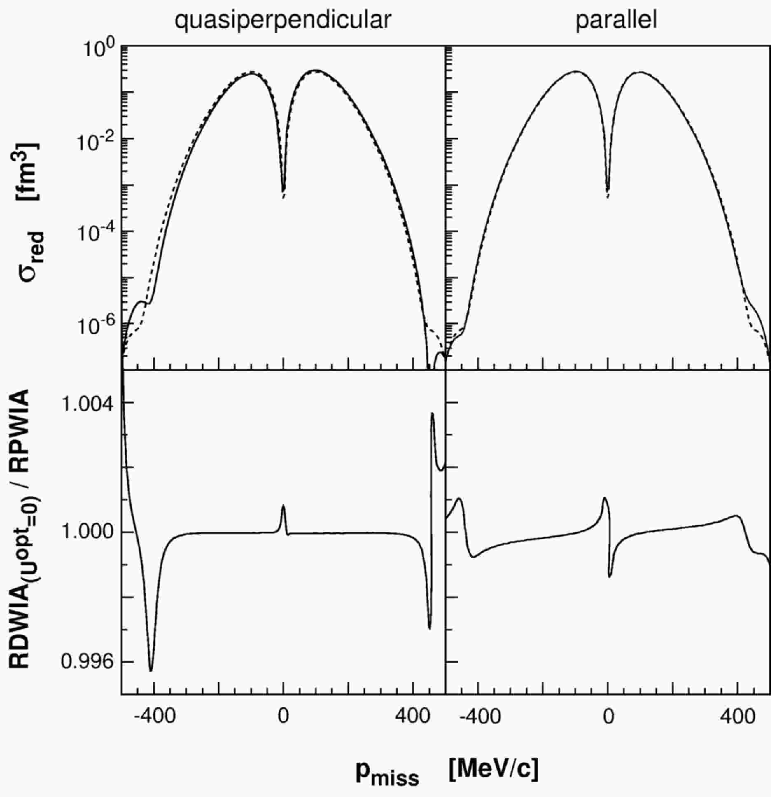
Figure 7: Comparisons between rpwia and rdwia${}_{\rm(U^{opt}=0)}$ calculations for the removal of protons from the $1p_{1/2}$-state of ¹⁶O as a function of $p_{\rm miss}$ for $E_{\rm beam}$ = 2.442 GeV. In the upper panels, the solid curves represent the reduced cross sections for both the rdwia${}_{\rm(U^{opt}=0)}$ and the rpwia calculations (see text for details). The dashed curves correspond to the momentum distributions. In the lower panels, rdwia${}_{\rm(U^{opt}=0)}$ / rpwia reduced cross-section ratios are shown. Agreement to much better than 1% is obtained for both kinematics over the entire $p_{\rm miss}$ range.

The rdwia${}_{\rm(U^{opt}=0)}$ calculations employed a partial-wave expansion of the second-order Dirac equation with optical potentials nullified and the target mass artificially set to 16001$u$ to minimize recoil corrections and frame ambiguities. The rpwia calculations (see Ref. Amaldi et al. (1967)) are based upon the Fourier transforms of the upper and lower components of the overlap function; that is, no partial-wave expansion is involved. In the upper panels, the solid curves represent the reduced cross section for both the rdwia${}_{\rm(U^{opt}=0)}$ and rpwia calculations as the differences are indistinguishable on this scale. The dashed curves show the momentum distributions. In the lower panels, the ratios between rdwia${}_{\rm(U^{opt}=0)}$ and rpwia reduced cross sections are shown. With suitable choices for step size and maximum $\ell$ (here 0.05 fm and 80), agreement to much better than $1\%$ over the entire range of missing momentum is obtained, verifying the accuracy of LEA for plane waves. Similar results are obtained with the Madrid code.

The similarity between the reduced cross sections and the momentum distributions demonstrates that the violation of factorization produced by the distortion of the bound-state spinor is mild, but tends to increase with $p_{\rm miss}$. Nevertheless, observables such as $A_{LT}$ that are sensitive to the interference between the lower and upper components are more strongly affected by violation of factorization.

Figs. 8 and 9 compare calculations for the removal of protons from the $1p$-shell of ¹⁶O as a function of $p_{\rm miss}$ for $E_{\rm beam}$ = 2.442 GeV. These predictions were made by Kelly Kelly (2003) using the LEA and the Madrid codes with identical input options, and are hereafter described as ‘baseline’ calculations. The baseline options are summarized in Table 5 and were chosen to provide the most rigorous test of the codes rather than to be the optimal physics choices.

Table 5: A summary of the basic rdwia options which served as input to the ‘baseline’ comparison calculations of the Madrid Group and Kelly (LEA). Results are shown in Figs. 8 and 9.

Input Parameter	Option
bound-nucleon wave function	nlsh – Sharma et al. Sharma et al. (1993)
Optical Model	edai-o – Cooper et al. Cooper et al. (1993)
nucleon spinor distortion	relativistic
electron distortion	none
current operator	cc2
nucleon form factors	dipole
gauge	Coulomb

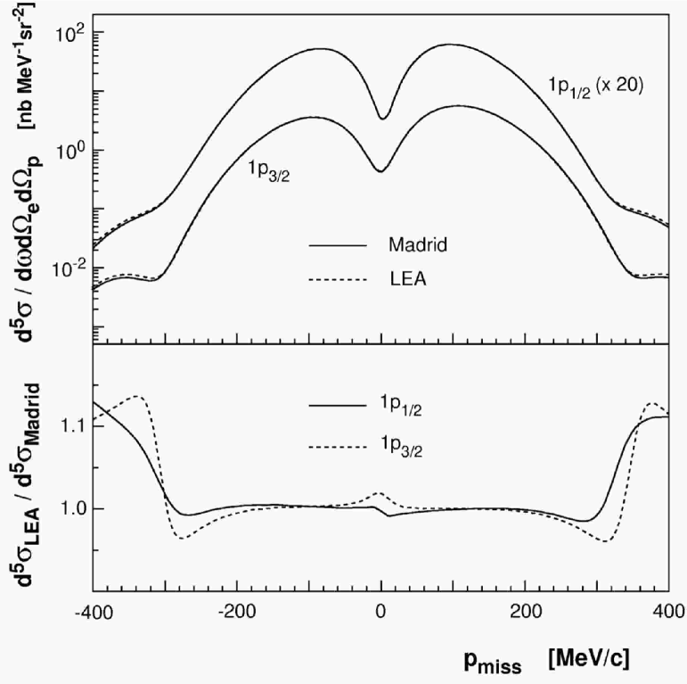
Figure 8: Comparison baseline rdwia calculations by the Madrid Group and Kelly (LEA) for the removal of protons from the 1$p$-shell of ¹⁶O as a function of $p_{\rm miss}$ for $E_{\rm beam}$ = 2.442 GeV. For the purposes of this comparison, the input into both calculations was identical (see Table 5). Overall agreement is very good, and agreement is excellent for $-$250 $<$ $p_{\rm miss}$ $<$ 250 MeV/$c$.

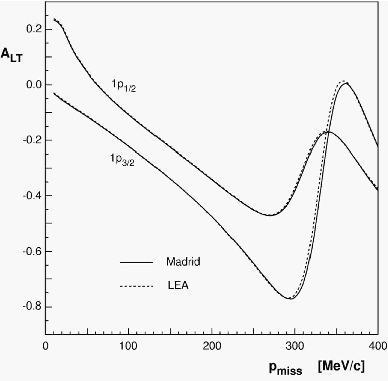
Figure 9: Comparison baseline rdwia calculations for the $A_{LT}$ asymmetry by the Madrid Group and Kelly (LEA) for the removal of protons from the 1$p$-shell of ¹⁶O as a function of $p_{\rm miss}$ for $E_{\rm beam}$ $=$ 2.442 GeV. For the purposes of this comparison, the input into both calculations was identical (see Table 5). Overall agreement is excellent over the entire $p_{\rm miss}$ range.

Fig. 8 demonstrates that baseline cross-section calculations agree to better than $2\%$ for $p_{\rm miss}$ $<$ 250 MeV/$c$, but that the differences increase to about $10\%$ by about 400 MeV/$c$. Nevertheless, Fig. 9 shows that excellent agreement is obtained for $A_{LT}$ over this entire range of $p_{\rm miss}$, with only a very small observable shift. The agreement of the strong oscillations in $A_{LT}$ for $p_{\rm miss}$ $\approx$ 300 MeV/$c$ predicted by both methods demonstrates that they are equivalent with respect to spinor distortion. The small differences in the cross section for large $p_{\rm miss}$ appear to be independent of the input choices and probably arise from numerical errors in the integration of differential equations (perhaps due to initial conditions), but the origin has not yet been identified. Regardless, it is remarkable to achieve this level of agreement between two independent codes under conditions in which the cross section spans three orders of magnitude.

IV.2 ROMEA / RMSGA

In this subsection, an alternate relativistic model developed by the Ghent Group Debruyne et al. (2000); Debruyne and Ryckebusch (2002); Debruyne et al. (2002); Ryckebusch et al. (2003) for $A(e,e^{\prime}N)B$ processes is presented. With respect to the construction of the bound-nucleon wave functions and the nuclear-current operator, an approach similar to standard rdwia is followed. The major differences lie in the construction of the scattering wave function. The approach presented here adopts the relativistic Eikonal Approximation (EA) to determine the scattering wave functions and may be used in conjunction with either the Optical Model or the multiple-scattering Glauber frameworks for dealing with the FSI.

IV.2.1 Formalism

The EA belongs to the class of semi-classical approximations which are meant to become ‘exact’ in the limit of small de Broglie ($db$) wavelengths, $\lambda_{db}\ll a$, where $a$ is the typical range of the potential in which the particle is moving. For a particle moving in a relativistic (optical) potential consisting of scalar and vector terms, the scattering wave function takes on the EA form

$$\psi_{F}(\bm{r}\hskip 1.42262pt)\sim\left[\begin{array}[]{c}1\\ \frac{1}{E+m+S-V}~{}\bm{\sigma}\cdot\bm{p}\end{array}\right]e^{i\bm{p}\cdot\bm{r}}{e^{i{\cal S}(\bm{r})}}\chi_{m_{s}}\;.$$ (33)

This wave function differs from a relativistic plane wave in two respects: first, there is a dynamical relativistic effect from the scalar ($S$) and vector ($V$) potentials which enhances the contribution from the lower components; and second, the wave function contains an eikonal phase which is determined by integrating the central ($U^{C}$) and spin-orbit ($U^{LS}$) terms of the distorting potentials along the (asymptotic) trajectory of the escaping particle. In practice, this amounts to numerically calculating the integral ($\bm{r}\equiv(\bm{b},z)$)

$$i{\cal S}(\bm{b},z) = -i\frac{m}{K}\int_{-\infty}^{z}dz^{\prime}\,\biggl{[}{U^{C}(\bm{b},z^{\prime})}$$ (34)

$$+{U^{LS}(\bm{b},z^{\prime})}[\bm{\sigma}\cdot(\bm{b}\times\bm{K})-iKz^{\prime}\hskip 0.7113pt]\biggr{]}\;,$$

where $\bm{K}\equiv\frac{1}{2}\left(\bm{p}+\bm{q}\hskip 0.7113pt\right)$.

Within the romea calculation, the eikonal phase given by Eq. (34) is computed from the relativistic optical potentials as they are derived from global fits to elastic proton-nucleus scattering data. It is worth stressing that the sole difference between the romea and the rdwia models is the use of the EA to compute the scattering wave functions.

For proton lab momenta exceeding 1  GeV/$c$, the highly inelastic nature of the elementary nucleon-nucleon ($NN$) scattering process makes the use of a potential method for describing FSI effects somewhat artificial. In this high-energy regime, an alternate description of FSI processes is provided by the Glauber Multiple-Scattering Theory. A relativistic and unfactorized formulation of this theory has been developed by the Ghent Group Debruyne et al. (2002); Ryckebusch et al. (2003). In this framework, the $A$-body wave function in the final state reads

$$\Psi^{\bm{p}}_{A}\left(\bm{r},\bm{r}_{2},\bm{r}_{3},\ldots\bm{r}_{A}\right) \sim {\widehat{\mathcal{O}}}\left[\begin{array}[]{c}1\\ \frac{1}{E+m}~{}\bm{\sigma}\cdot\bm{p}\end{array}\right]e^{i\bm{p}\cdot\bm{r}}\chi_{m_{s}}$$ (38)

$$\times\Psi_{B}\left(\bm{r}_{2},\ldots\bm{r}_{A}\right)\;,$$

where $\Psi_{B}$ is the wave function characterizing the state in which the $B$ nucleus is created. In the above expression, the subsequent elastic or ‘mildly inelastic’ collisions which the ejectile undergoes with ‘frozen’ spectator nucleons are implemented through the introduction of the operator

$${\widehat{\mathcal{O}}\left(\bm{r},\bm{r}_{2},\bm{r}_{3},\ldots\bm{r}_{A}\right)}\equiv\prod_{j=2}^{A}\left[1-\Gamma\left({p},\bm{b}-\bm{b_{j}}\right)\theta\left(z-z_{j}\right)\right]~{},$$

where the profile function for $pN$ scattering is

$$\Gamma(p,\bm{b})=\frac{{\sigma^{\rm tot}_{pN}}(1-i{\epsilon_{pN}})}{4\pi\beta_{pN}^{2}}\>\exp\left(-\frac{b^{2}}{2\beta_{pN}^{2}}\right)\;.$$

In practice, for the lab momentum of a given ejectile, the following input is required: the total proton-proton and proton-neutron cross section ${\sigma^{\rm tot}_{pN}}$, the slope parameters ${\beta_{pN}}$, and the ratio of the real-to-imaginary scattering amplitude ${\epsilon_{pN}}$. The parameters ${\sigma^{\rm tot}_{pN}}$, ${\beta_{pN}}$, and ${\epsilon_{pN}}$ are obtained through interpolation of the data base made available by the Particle Data Group Hagiwara et al. (2002). The $A(e,e^{\prime}N)B$ results obtained with a scattering state of the form of Eq. (38) are referred to as rmsga calculations. It is worth stressing that in contrast to the rdwia and the romea models, all parameters entering the calculation of the scattering states in rmsga are directly obtained from the elementary proton-proton and proton-neutron scattering data. Thus, the scattering states are not subject to the $SV$ effects discussed in Section IV.1.1, which typically arise when relativistic potentials are employed. However, the $SV$ effects are included for the bound-state wave function.

Note that for the kinematics of the ¹⁶O$(e,e^{\prime}p)$ experiment presented in this paper, the de Broglie wavelength of the ejected proton is $\lambda_{db}\approx 1.3$ fm, and thus both the optical potential and the Glauber frameworks may be applicable. Indeed, for $T_{p}\approx 0.433$ GeV, various sets of relativistic optical potentials are readily available and $\lambda_{db}$ appears sufficiently small for the approximations entering the Glauber framework to be justifiable – see Ref. Debruyne et al. (2002).

IV.2.2 Tests

As previously mentioned, the (rdwia and romea) and rmsga frameworks are substantially different in the way they address FSI. While the rdwia and romea models are both essentially one-body approaches in which all FSI effects are implemented through effective potentials, the rmsga framework is a full-fledged, multi-nucleon scattering model based on the EA and the concept of frozen spectators. As such, when formulated in an unfactorized and relativistic framework, Glauber calculations are numerically involved and the process of computing the scattering state and the transition matrix elements involves numerical methods which are different from those adopted in rdwia frameworks. For example, for $A(e,e^{\prime}N)B$ calculations in the romea and the rmsga, partial-wave expansions are simply not a viable option.

The testing of the mutual consistency of the rdwia and ‘bare’ rmsga (no MEC nor IC) calculations began by considering the special case of vanishing FSI. In this limit, where all the Glauber phases are nullified in rmsga and (rdwia $\rightarrow$ rpwia), the two calculations were determined to reproduce one another to 4% over the entire $p_{\rm miss}$ range, thereby establishing the validity of the numerics. The Glauber phases were then enabled. The basic options which then served as input to the comparison between the rdwia calculations and the rmsga calculations of the Ghent Group Ryckebusch and Debruyne (2002) are presented in Table 6.

Table 6: A summary of the basic options which served as input to the comparison between the rdwia calculations and the ‘bare’ rmsga (no MEC nor IC) calculations of the Ghent Group. Results are shown in Fig. 10.

Input Parameter	Option
bound-nucleon wave function	Furnstahl et al. Furnstahl et al. (1997)
Optical Model	edai-o
nucleon spinor distortion	relativistic
electron distortion	none
current operator	cc2
nucleon form factors	dipole
gauge	Coulomb

Fig. 10 shows the ratio of the bare rmsga calculations of the Ghent Group together with rdwia calculations for the removal of protons from the 1$p$-shell of ¹⁶O as a function of $p_{\rm miss}$ for $E_{\rm beam}$ = 2.442 GeV. Apart from the treatment of FSI, all other ingredients to the calculations are identical (see Table 6). For $p_{\rm miss}$ below the Fermi momentum, the variation between the predictions of the two approaches is at most 25%, with the rdwia approach predicting a smaller cross section (stronger absorptive effects) than the rmsga model. Not surprisingly, at larger $p_{\rm miss}$ (correspondingly larger polar angles), the differences between the two approaches grow.

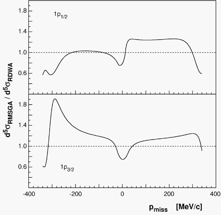
Figure 10: rdwia calculations compared to ‘bare’ (no MEC nor IC) rmsga calculations by the Ghent Group for the removal of protons from the 1$p$-shell of ¹⁶O as a function of $p_{\rm miss}$ for $E_{\rm beam}$ = 2.442 GeV. Both calculations employ the input presented in Table 6. Apart from the treatment of FSI, all ingredients are identical.

V Results for $\bm{Q^{2}\approx 0.8}$ (GeV/$\bm{c}$)²

The data were interpreted in subsets corresponding to the 1$p$-shell and to the 1$s_{1/2}$-state and continuum. The interested reader is directed to the works of Gao et al. Gao et al. (2000) and Liyanage et al. Liyanage et al. (2001), where these results have been briefly highlighted. Note that when data are presented in the following discussion, statistical uncertainties only are shown. A complete archive of the data, including systematic uncertainties, is presented in Appendix A.

V.1 $\bm{1p}$-shell knockout

V.1.1 Sensitivity to rdwia variations

The consistency of the normalization factors $S_{\alpha}$ suggested by the $1p$-shell data for $p_{\rm miss}$ $<$ 350 MeV/$c$ obtained in this measurement at 2.442 GeV (see Table LABEL:table:pshellperpresults) was examined within the rdwia framework in a detailed study by the Madrid Group Udías and Vignote (2001). The study involved systematically varying a wide range of inputs to the rdwia calculations, and then performing least-squares fits of the predictions to the cross-section data. The results of the study are presented in Table 7.

Table 7: Normalization factors derived from the 2.442 GeV $1p$-shell cross-section data of Table LABEL:table:pshellperpresults using the cc1 and cc2 current operators. The first term in each column is for the $1p_{1/2}$-state, while the second term is for the $1p_{3/2}$-state.

			bound-											nucleon
			nucleon						optical					FF			doublet
prescription			wavefunction			gauge			potential					model			(%)			Sα				$\chi^{2}$
fully		EMA-	nls						eda							gk+
rel	proj	noSV	h	h-p	hs	C	W	L	i-o	d1	d2	mrw	rlf	gk	d	qmc	100	50	0	cc1		cc2		cc1		cc2
*			*			*			*					*			*			0.68	0.62	0.74	0.67	5.5	5.3	2.0	31.0
	*		*			*			*					*			*			0.78	0.73	0.76	0.71	17.0	79.0	8.0	70.0
		*	*			*			*					*			*			0.72	0.66	0.75	0.69	2.3	65.0	2.2	65.0
*				*		*			*					*			*			0.60	0.52	0.63	0.54	10.0	97.0	15.0	115.0
					*	*			*					*			*			0.62	0.61	0.65	0.65	10.0	6.7	18.0	41.0
*			*				*		*					*			*			0.63	0.59	0.76	0.70	25.0	9.2	2.6	22.0
			*					*	*					*			*			0.69	0.63	0.73	0.67	3.7	6.4	2.5	34.0
*			*			*				*				*			*			0.64	0.60	0.72	0.67	29.0	12.0	4.8	8.2
			*			*					*			*			*			0.64	0.59	0.71	0.65	15.0	6.4	0.7	15.0
			*			*						*		*			*			0.62	0.60	0.71	0.67	35.0	11.0	7.6	7.3
			*			*							*	*			*			0.61	0.58	0.70	0.65	41.0	12.0	6.1	7.9
*			*			*			*						*		*			0.69	0.63	0.75	0.68	4.8	5.9	2.1	31.0
			*			*			*							*	*			0.65	0.61	0.72	0.66	11.0	3.3	0.5	16.0
*			*			*			*					*				*			0.64		0.70		6.1		33.0
			*			*			*					*					*		0.66		0.72		7.4		35.0

Three basic approaches were considered: the fully relativistic approach, the projected approach of Udías et al. Udías et al. (1999); Udías and Vignote (2000), and the EMA-noSV approach of Kelly Kelly (1997, 1999b). All three approaches included the effects of electron distortion. While the fully relativistic approach involved solving the Dirac equation directly in configuration space, the projected approach included only the positive-energy components, and as a result, most (but not all) of the spinor distortion was removed from the wave functions. Within the EMA-noSV approach, a relativized Schrödinger equation was solved using the EMA, and all of the spinor distortion was removed. This made the calculation similar to a factorized calculation, although spin–orbit effects in the initial and final states (which cause small deviations from the factorized results) are included in EMA-noSV.

The current operator was changed between cc1 and cc2. Three bound-nucleon wave functions (see Fig. 11) derived from relativistic Lagrangians were considered: hs by Horowitz and Serot Horowitz and Serot (1981); Horowitz et al. (1991), nlsh by Sharma et al. Sharma et al. (1993), and nlsh-p by Udías et al. Udías et al. (2001) (which resulted from a Lagrangian fine-tuned to reproduce the Leuschner et al. data). Note that both the nlsh and nlsh-p wave functions predict binding energies, single-particle energies, and a charge radius for ¹⁶O which are all in good agreement with the data.

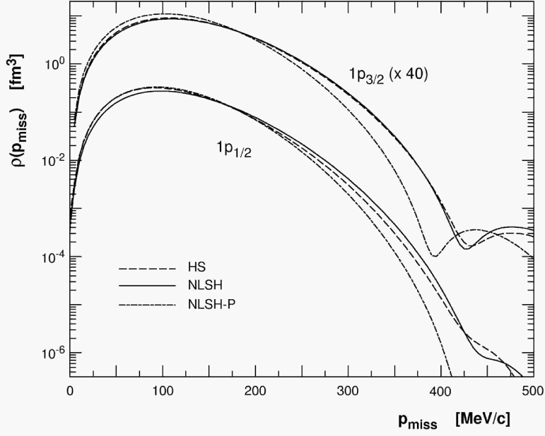
Figure 11: Momentum distributions for the hs, nlsh, and nlsh-p models. There is only a slight difference between hs and nlsh – for the $1p_{3/2}$-state, hs is broader spatially and thus drops off faster with increasing $p_{\rm miss}$. On the other hand, nlsh-p differs appreciably from both hs and nlsh, and is clearly distinguishable for $p_{\rm miss}$ $>$ 250 MeV/$c$ for both the $1p_{1/2}$- and $1p_{3/2}$-states. Note that both the nlsh and nlsh-p wave functions predict binding energies, single-particle energies, and a charge radius for ¹⁶O which are all in good agreement with the data.

The gauge prescription was changed between Coulomb, Weyl, and Landau. The nucleon distortion was evaluated using three purely phenomenological $SV$ optical potentials (edai-o, edad1, and edad2) by Cooper et al. Cooper et al. (1993), as well as mrw by McNeil et al. McNeil et al. (1983) and rlf by Horowitz Horowitz (1985) and Murdock Murdock (1987). The nucleon form-factor model was changed between gk by Gari and Krümpelmann Gari and Krümpelmann (1985) and the dipole model. Further, the qmc model of Lu et al. Lu et al. (1998, 1999) predicts a density dependence for form factors that was calculated and applied to the gk form factors using the LDA (see Ref. Kelly (1999a)).

Note that the calculations for the $1p_{3/2}$-state include the incoherent contributions of the unresolved $2s_{1/2}1d_{5/2}$-doublet. The bound-nucleon wave functions for these positive-parity states were taken from the parametrization of Leuschner et al. and normalization factors were fit to said data using rdwia calculations. Factors for both states of 0.12(3) relative to full occupancy were determined. The sensitivity of the present data to this incoherent admixture was evaluated by scaling the fitted doublet contribution using factors of 0.0, 0.5, and 1.0.

Qualitatively, the fully relativistic approach clearly did the best job of reproducing the data. Fully relativistic results were shown to be much less gauge-dependent than the nonrelativistic results. The cc2 current operator was in general less sensitive to choice of gauge, and the data discouraged the choice of the Weyl gauge. The different optical models had little effect on the shape of the calculations, but instead changed the overall magnitude. Both the gk and dipole nucleon form-factor models produced nearly identical results. The change in the calculated gk+qmc cross section was modest, being most pronounced in $A_{LT}$ for $p_{\rm miss}$ $>$ 300 MeV/$c$. The results were best for a 100% contribution of the strength of the $2s_{1/2}1d_{5/2}$-doublet to the $1p_{3/2}$-state, although the data were not terribly sensitive to this degree of freedom.

Fig. 12 shows the left-right asymmetry $A_{LT}$ together with rdwia calculations for the removal of protons from the $1p$-shell of ¹⁶O as a function of $p_{\rm miss}$ for $E_{\rm beam}$ $=$ 2.442 GeV. The origin of the large change in the slope of $A_{LT}$ at $p_{\rm miss}$ $\approx$ 300 MeV/$c$ is addressed by the various calculations. This ‘ripple’ effect is due to the distortion of the bound-nucleon and ejectile spinors, as evidenced by the other three curves shown, in which the full rdwia calculations have been decomposed. It is important to note that these three curves all retain the same basic ingredients, particularly the fully relativistic current operator and the upper components of the Dirac spinors. Of the three curves, the dotted line resulted from a calculation where only the bound-nucleon spinor distortion was included, the dashed line resulted from a calculation where only the scattered-state spinor distortion was included, and the dashed-dotted line resulted from a calculation where undistorted spinors (essentially identical to a factorized calculation) were considered. Clearly, the inclusion of the bound-nucleon spinor distortion is more important than the inclusion of the scattered-state spinor distortion, but both are necessary to describe the data.

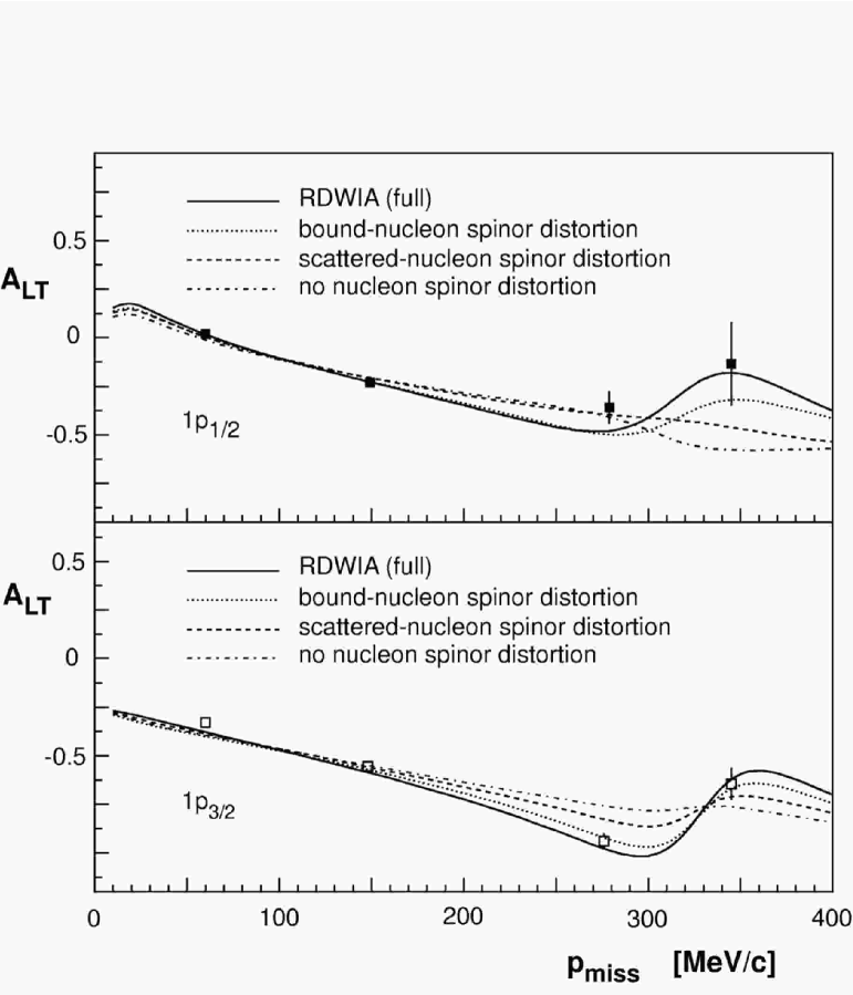
Figure 12: Left-right asymmetry $A_{LT}$ together with rdwia calculations for the removal of protons from the 1$p$-shell of ¹⁶O as a function of $p_{\rm miss}$ for $E_{\rm beam}$ $=$ 2.442 GeV. Uncertainties are statistical (see Table LABEL:table:pshellaltrlt for the associated systematic uncertainties). Note that the solid curves shown here are identical to those shown in Figs. 13 and 15.

The effects of variations in the ingredients to the calculations of the left-right asymmetry $A_{LT}$ for the $1p_{1/2}$-state only are shown in Fig. 13. Note that the data are identical to those presented in Fig. 12, as are the solid curves. In the top panel, the edai-o optical potential and nlsh bound-nucleon wave function were used for all the calculations, but the choice of current operator was varied between cc1 (dashed), cc2 (solid), and cc3 (dashed-dotted), resulting in a change in both the height and the $p_{\rm miss}$-location of the ripple in $A_{LT}$. In the middle panel, the current operator cc2 and edai-o optical potential were used for all the calculations, but the choice of bound-nucleon wave function was varied between nlsh-p (dashed), nlsh (solid), and hs (dashed-dotted), resulting in a change in the $p_{\rm miss}$-location of the ripple, but a relatively constant height. In the bottom panel, the current operator cc2 and nlsh bound-nucleon wave function were used for all the calculations, but the choice of optical potential was varied between edad1 (dashed), edai-o (solid), and edad2 (dashed-dotted), resulting in a change in the height of the ripple, but a relatively constant $p_{\rm miss}$-location. More high-precision data, particularly for 150 $<$ $p_{\rm miss}$ $<$ 400 MeV/$c$, are clearly needed to accurately and simultaneously determine the current operator, the bound-state wave function, the optical potential, and of course the normalization factors. This experiment has recently been performed in Hall A at Jefferson Lab by Saha et al. Saha et al. (2000), and the results are currently under analysis.

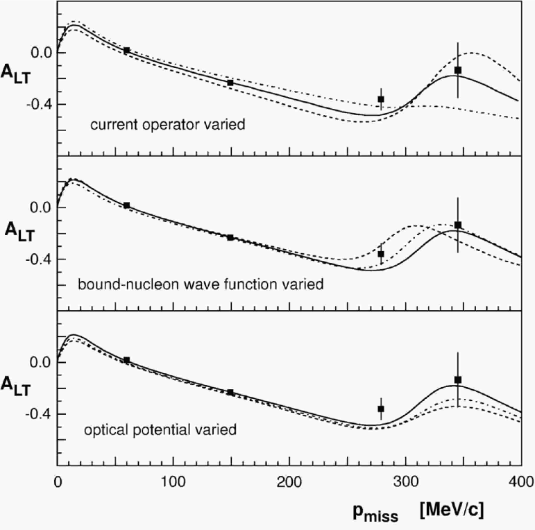
Figure 13: Left-right asymmetry $A_{LT}$ together with rdwia calculations for the removal of protons from the 1$p_{1/2}$-state of ¹⁶O as a function of $p_{\rm miss}$ for $E_{\rm beam}$ $=$ 2.442 GeV. Uncertainties are statistical (see Table LABEL:table:pshellaltrlt for the associated systematic uncertainties). The solid curves in all three panels are the same and are identical to those shown for the removal of protons from the 1$p_{1/2}$-state of ¹⁶O in Figs. 12 and 15.

V.1.2 Comparison to rdwia, romea, and rmsga calculations considering single-nucleon currents

In this Section, the data are compared to rdwia and bare romea and rmsga calculations (which take into consideration single-nucleon currents only – no MEC or IC). The basic options employed in the calculations are summarized in Table 8. Note that both the EA-based calculations stop at $p_{\rm miss}$ $=$ 350 MeV/$c$ as the approximation becomes invalid.

Table 8: A summary of the basic options which served as input to the single-nucleon current rdwia, romea, and rmsga comparison calculations. Results are shown in Figs. 14 – 16.

		romea
Input Parameter	rdwia	& rmsga
bound-nucleon wave function	nlsh	hs
Optical Model	edai-o	edai-o
nucleon spinor distortion	relativistic	relativistic
electron distortion	yes	yes
current operator	cc2	cc2
nucleon form factors	gk	dipole
gauge	Coulomb	Coulomb

Fig. 14 shows measured cross-section data for the removal of protons from the 1$p$-shell of ¹⁶O as a function of $p_{\rm miss}$ as compared to relativistic calculations at $E_{\rm beam}$ = 2.442 GeV. The solid line is the rdwia calculation, while the dashed and dashed-dotted lines are respectively the bare romea and rmsga calculations. The normalization factors for the rdwia calculations are 0.73 and 0.72 for the $1p_{1/2}$-state and $1p_{3/2}$-state, respectively. For the romea and rmsga calculations, they are 0.6 and 0.7 for the $1p_{1/2}$-state and $1p_{3/2}$-state, respectively. The rdwia calculations do a far better job of representing the data over the entire $p_{\rm miss}$ range.

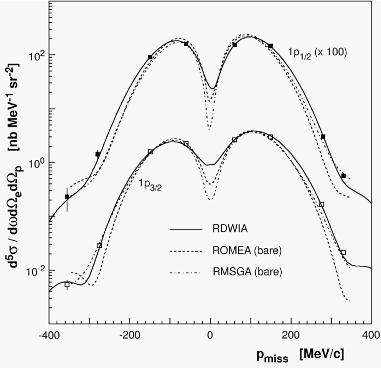
Figure 14: Measured cross-section data for the removal of protons from the 1$p$-shell of ¹⁶O as a function of $p_{\rm miss}$ as compared to relativistic calculations at $E_{\rm beam}$ = 2.442 GeV. Uncertainties are statistical and, on average, there is an additional $\pm$5.6% systematic uncertainty (see Table LABEL:table:pshellperpresults) associated with the data. The solid line is the rdwia calculation, while the dashed and dashed-dotted lines are respectively the bare romea and rmsga calculations.

Fig. 15 shows the left-right asymmetry $A_{LT}$ together with relativistic calculations for the removal of protons from the 1$p$-shell of ¹⁶O as a function of $p_{\rm miss}$ for $E_{\rm beam}$ = 2.442 GeV. The solid line is the rdwia calculation, while the dashed and dashed-dotted lines are respectively the bare romea and rmsga calculations. Note again the large change in the slope of $A_{LT}$ at $p_{\rm miss}$ $\approx$ 300 MeV/$c$. While all three calculations undergo a similar change in slope, the rdwia calculation does the best job of reproducing the data. The romea calculation reproduces the data well for $p_{\rm miss}$ $<$ 300 MeV/$c$, but substantially overestimates $A_{LT}$ for $p_{\rm miss}$ $>$ 300 MeV/$c$. The rmsga calculation does well with the overall trend in the data, but struggles with reproducing the data for the $1p_{1/2}$-state.

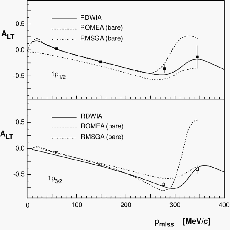
Figure 15: Left-right asymmetry $A_{LT}$ together with relativistic calculations of the $A_{LT}$ asymmetry for the removal of protons from the 1$p$-shell of ¹⁶O as a function of $p_{\rm miss}$ for $E_{\rm beam}$ = 2.442 GeV. Uncertainties are statistical (see Table LABEL:table:pshellaltrlt for the associated systematic uncertainties). The solid line is the rdwia calculation, while the dashed and dashed-dotted lines are respectively the bare romea and rmsga calculations. Note that the solid curves shown here are identical to those shown in Figs. 12 and 13.

Fig. 16 shows the $R_{L+TT}$, $R_{LT}$, and $R_{T}$ effective response functions together with relativistic calculations for the removal of protons from the 1$p$-shell of ¹⁶O as a function of $p_{\rm miss}$. Note that the data point located at $p_{\rm miss}$ $\approx$ 52 MeV/$c$ comes from the parallel kinematics measurements (see Table LABEL:table:pshellrlrt), while the other data points come from the quasiperpendicular kinematics measurements (see Tables LABEL:table:pshellrlttrt and LABEL:table:pshellaltrlt). The solid line is the rdwia calculation, while the dashed and dashed-dotted lines are respectively the bare romea and rmsga calculations. The agreement, particularly between the rdwia calculations and the data, is very good. The spinor distortions in the rdwia calculations which were required to predict the change in slope of $A_{LT}$ at $p_{\rm miss}$ $\approx$ 300 MeV/$c$ in Fig. 12 are also essential to the description of $R_{LT}$. The agreement between the rmsga calculations and the data, particularly for $R_{LT}$, is markedly poorer.

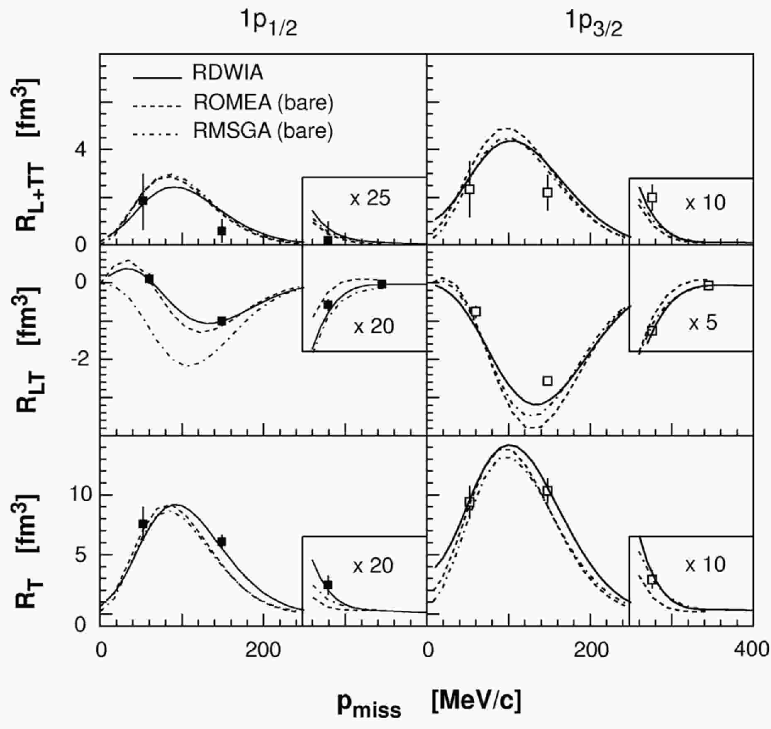
Figure 16: Data from this work together with relativistic calculations for the $R_{L+TT}$, $R_{LT}$, and $R_{T}$ effective response functions for the removal of protons from the 1$p$-shell of ¹⁶O as a function of $p_{\rm miss}$. Uncertainties are statistical (see Tables LABEL:table:pshellrlttrt, LABEL:table:pshellaltrlt, and LABEL:table:pshellrlrt for the associated systematic uncertainties). The solid line is the rdwia calculation, while the dashed and dashed-dotted lines are respectively the bare romea and rmsga calculations.

Qualitatively, it should again be noted that none of the calculations presented so far have included contributions from two-body currents. The good agreement between the calculations and the data indicates that these currents are already small at $Q^{2}$ $\approx$ 0.8 (GeV/$c$)². This observation is supported by independent calculations by Amaro et al. Amaro et al. (1999, 2003) which estimate the importance of such currents (which are highly dependent on $p_{\rm miss}$) to be large at lower $Q^{2}$, but only 2% for the $1p_{1/2}$-state and 8% for the $1p_{3/2}$-state in these kinematics. It should also be noted that the rdwia results presented here are comparable with those obtained in independent rdwia analyses of our data by the Pavia Group – see Meucci et al. Meucci et al. (2001)

V.1.3 Comparison to romea and rmsga calculations including two-body currents

In this Section, two-body current contributions to the romea and rmsga calculations stemming from MEC and IC are presented. These contributions to the transition matrix elements were determined within the nonrelativistic framework outlined by the Ghent Group in Ryckebusch et al. (1999); Ryckebusch (2001). Recall that the basic options employed in the calculations have been summarized in Table 8. Note again that both the EA-based calculations stop at $p_{\rm miss}$ $=$ 350 MeV/$c$ as the approximation becomes invalid.

Fig. 17 shows measured cross-section data for the removal of protons from the 1$p$-shell of ¹⁶O as a function of $p_{\rm miss}$ as compared to calculations by the Ghent Group which include MEC and IC at $E_{\rm beam}$ = 2.442 GeV. In the top panel, romea calculations are shown. The dashed line is the bare calculation, the dashed-dotted line includes MEC, and the solid line includes both MEC and IC. In the bottom panel, rmsga calculations are shown. The dashed line is the bare calculation, the dashed-dotted line includes MEC, and the solid line includes both MEC and IC. Note that the curves labelled ‘bare’ in this figure are identical to those shown in Fig. 14. The normalization factors are 0.6 and 0.7 for the $1p_{1/2}$-state and $1p_{3/2}$-state, respectively. The impact of the two-body currents on the computed differential cross section for the knockout of 1$p$-shell protons from ¹⁶O is no more than a few percent for low $p_{\rm miss}$, but gradually increases with increasing $p_{\rm miss}$. Surprisingly, explicit inclusion of the two-body current contributions to the transition matrix elements does not markedly improve the overall agreement between the calculations and the data.

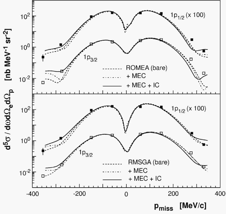
Figure 17: Measured cross-section data for the removal of protons from the 1$p$-shell of ¹⁶O as a function of $p_{\rm miss}$ together with calculations by the Ghent Group at $E_{\rm beam}$ = 2.442 GeV. Uncertainties are statistical and, on average, there is an additional $\pm$5.6% systematic uncertainty (see Table LABEL:table:pshellperpresults). The curves labelled ‘bare’ are identical to those shown in Fig. 14.

Fig. 18 shows the left-right asymmetry $A_{LT}$ together with calculations by the Ghent Group for the removal of protons from the 1$p$-shell of ¹⁶O as a function of $p_{\rm miss}$ for $E_{\rm beam}$ $=$ 2.442 GeV. In the top two panels, romea calculations are shown. The dashed lines are the bare calculations identical to those previously shown in Fig. 15, the dashed-dotted line includes MEC, and the solid line includes both MEC and IC. In the bottom panel, rmsga calculations are shown. The dashed line is the bare calculation, the dashed-dotted line includes MEC, and the solid line includes both MEC and IC. While all three calculations undergo a change in slope at $p_{\rm miss}$ $\approx$ 300 MeV/$c$, it is again clearly the bare calculations which best represent the data. Note that in general, the IC were observed to produce larger effects than the MEC.

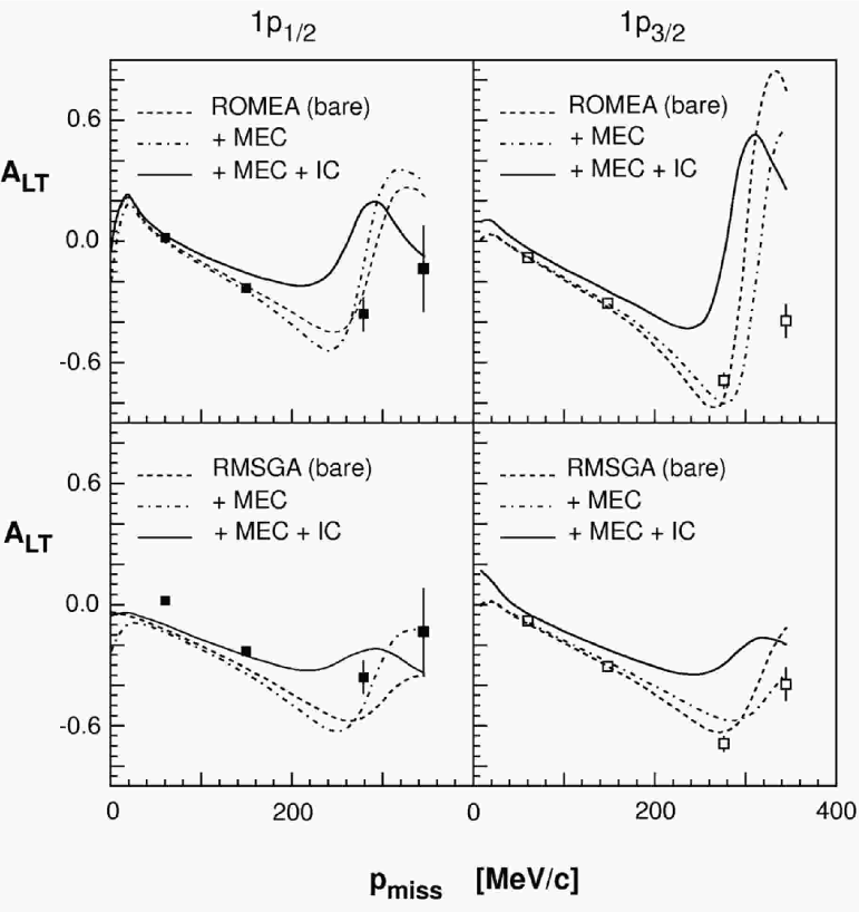
Figure 18: Left-right asymmetry $A_{LT}$ together with calculations by the Ghent Group of the $A_{LT}$ asymmetry for the removal of protons from the 1$p$-shell of ¹⁶O as a function of $p_{\rm miss}$ for $E_{\rm beam}$ = 2.442 GeV. Error bars are statistical (see Table LABEL:table:pshellaltrlt for the associated systematic uncertainties). The curves labelled ‘bare’ are identical to those shown in Fig. 15.

Figs. 19 and 20 show the effective $R_{L+TT}$, $R_{LT}$, and $R_{T}$ response functions together with romea and rmsga calculations by the Ghent Group for the removal of protons from the 1$p$-shell of ¹⁶O as a function of $p_{\rm miss}$. The dashed lines are the bare romea and rmsga calculations identical to those previously shown in Fig. 16, while the solid lines include both MEC and IC. In contrast to the cross-section (recall Fig. 17) and $A_{LT}$ (recall Fig. 18) situations, the agreement between the effective response-function data and the calculations improves with the explicit inclusion of the two-body current contributions to the transition matrix elements.

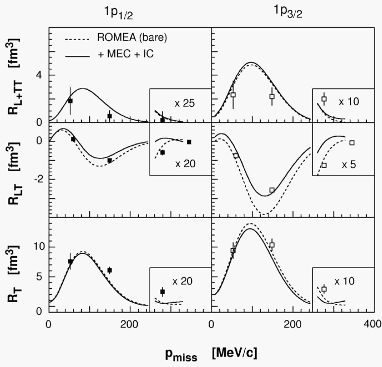
Figure 19: Data from this work together with romea calculations by the Ghent Group for the $R_{L+TT}$, $R_{LT}$, and $R_{T}$ effective response functions for the removal of protons from the 1$p$-shell of ¹⁶O as a function of $p_{\rm miss}$. Uncertainties are statistical (see Tables LABEL:table:pshellrlttrt, LABEL:table:pshellaltrlt, and LABEL:table:pshellrlrt for the associated systematic uncertainties). The curves labelled ‘bare’ are identical to those shown in Fig. 16.

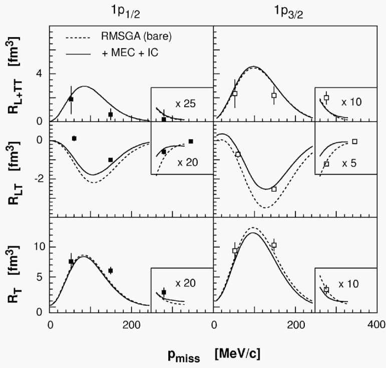
Figure 20: Data from this work together with rmsga calculations by the Ghent Group for the $R_{L+TT}$, $R_{LT}$, and $R_{T}$ effective response functions for the removal of protons from the 1$p$-shell of ¹⁶O as a function of $p_{\rm miss}$. Uncertainties are statistical (see Tables LABEL:table:pshellrlttrt, LABEL:table:pshellaltrlt, and LABEL:table:pshellrlrt for the associated systematic uncertainties). The curves labelled ‘bare’ are identical to those shown in Fig. 16.

V.2 Higher missing energies

In this Section, romea calculations are compared to the higher-$E_{\rm miss}$ data. The basic options employed in the calculations have been summarized in Table 8.

Fig. 21 presents averaged measured cross-section data as a function of $E_{\rm miss}$ obtained at $E_{\rm beam}$ $=$ 2.442 GeV for four discrete HRS_h angular settings ranging from 2.5^∘ $<$ $\theta_{pq}$ $<$ 20^∘, corresponding to average values of $p_{\rm miss}$ increasing from 50 to 340 MeV/$c$. The cross-section values shown are the averaged values of the cross section measured on either side of $\bm{q}$ at each $\theta_{pq}$. The strong peaks at $E_{\rm miss}$ $=$ 12.1 and 18.3 MeV correspond to $1p$-shell proton removal from ¹⁶O. As in Section V.1, the dashed curves corresponding to these peaks are the bare romea calculations, while the solid lines include both MEC and IC. The normalization factors remain 0.6 and 0.7 for the $1p_{1/2}$- and $1p_{3/2}$-states, respectively.

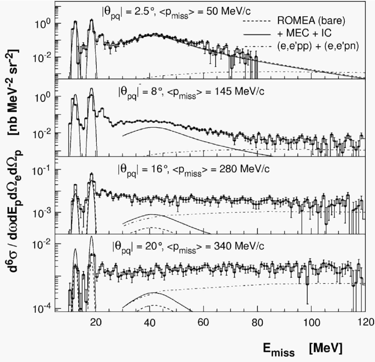
Figure 21: Data from this work together with romea calculations by the Ghent Group for the $E_{\rm miss}$-dependence of the cross section obtained at $E_{\rm beam}$ = 2.442 GeV. The data are the averaged cross section measured on either side of $\bm{q}$ at each $\theta_{pq}$. Normalization factors of 0.6, 0.7, and 1.0 have been used for the $1p_{1/2}$-, $1p_{3/2}$-, and $1s_{1/2}$-states, respectively. Uncertainties are statistical and, on average, there is an additional $\pm$5.9% systematic uncertainty (see Tables LABEL:table:2442cont000deg – LABEL:table:2442cont020deg) associated with the data. Also shown are calculations by the Ghent Group for the $(e,e^{\prime}pN)$ contribution.

For 20 $<$ $E_{\rm miss}$ $<$ 30 MeV, the spectra behave in a completely different fashion. Appreciable strength exists which scales roughly with the $1p$-shell fragments and is not addressed by the present calculations of two-nucleon knockout. The high-resolution experiment of Leuschner et al. identified two additional $1p_{3/2}$ fragments and several positive-parity states in this region which are populated primarily by single-proton knockout from $2p2h$ components of the ground-state wave function. Two-body currents and channel-coupling in the final state also contribute. This strength has also been studied in $(\gamma,p)$ experiments, and has been interpreted by the Ghent Group Ryckebusch et al. (1992) as the post-photoabsorption population of states with a predominant $1p2h$ character via two-body currents.

For $E_{\rm miss}$ $>$ 30 MeV, in the top panel for $p_{\rm miss}$ $=$ 50 MeV/$c$, there is a broad and prominent peak centered at $E_{\rm miss}$ $\approx$ 40 MeV corresponding largely to the knockout of $1s_{1/2}$-state protons. As can be seen in the lower panels, the strength of this peak diminishes with increasing $p_{\rm miss}$, and completely vanishes beneath a flat background by $p_{\rm miss}$ $=$ 280 MeV/$c$. For $E_{\rm miss}$ $>$ 60 MeV and $p_{\rm miss}$ $\geq$ 280 MeV/$c$, the cross section decreases only very weakly as a function of $p_{\rm miss}$, and is completely independent of $E_{\rm miss}$.

In order to estimate the amount of the cross section observed for $E_{\rm miss}$ $>$ 25 MeV that can be explained by the single-particle knockout of protons from the $1s_{1/2}$-state, the data were compared to the romea calculations of the Ghent Group. The dashed curves are the bare calculations, while the solid lines include both MEC and IC. A normalization factor of 1.0 for the $1s_{1/2}$-state single-particle strength was used. The two calculations are indistinguishable for $p_{\rm miss}$ $\leq$ 145 MeV/$c$, and the agreement between these calculations and the measured cross-section data is reasonable (see the top two panels of Fig. 21 where there is an identifiable $1s_{1/2}$-state peak at $E_{\rm miss}$ $\approx$ 40 MeV). At higher $p_{\rm miss}$ (where there is no clear $1s_{1/2}$-state peak at $E_{\rm miss}$ $\approx$ 40 MeV), the data are substantially larger than the calculated bare cross section. Inclusion of MEC and IC improves the agreement, but there is still roughly an order-of-magnitude discrepancy. The rdwia calculations demonstrate similar behavior. Thus, the $p_{\rm miss}$ $\geq$ 280 MeV/$c$ data are not dominated by single-particle knockout. Note that the magnitude of ($S_{T}-S_{L}$) is consistent with that anticipated based on the measurements of Ulmer et al. at $Q^{2}$ = 0.14 (GeV/$c$)² and Dutta et al. at $Q^{2}$ = 0.6 and 1.8 (GeV/$c$)². Together, these data suggest that transverse processes associated with the knockout of more than one nucleon decrease with increasing $Q^{2}$.

Also shown as dashed-dotted curves in Fig. 21 are the calculations by the Ghent Group Janssen et al. (2000) for the $(e,e^{\prime}pp)$ and $(e,e^{\prime}pn)$ contributions to the $(e,e^{\prime}p)$ cross section performed within a Hartree-Fock framework. This two-particle knockout cross section was determined using the Spectator Approximation, in a calculation which included MEC, IC, and both central short-range correlations (SRC) and tensor medium-range correlations. Note that in these kinematics, this calculation performed with SRC alone produced only 2% of the two-particle knockout cross section, while including both SRC and tensor correlations produced only 15% of the two-particle knockout cross section. The calculated two-particle knockout cross section is essentially transverse in nature, since the two-body currents are predominantly transverse. The calculated strength underestimates the measured cross section by about 50% but has the observed flat shape for $E_{\rm miss}$ $>$ 50 MeV. It is thus possible that heavier meson exchange and processes involving three (or more) nucleons could provide a complete description of the data.

The measured effective response functions $R_{L+TT}$, $R_{LT}$, and $R_{T}$ together with romea calculations for $p_{\rm miss}$ $=$ 145 MeV/$c$ and $p_{\rm miss}$ $=$ 280 MeV/$c$ are presented in Fig. 22. Kinematic overlap restricted separations to $E_{\rm miss}$ $<$ 60 MeV. The dashed curves are the bare romea calculations, while the solid curves include both MEC and IC. Also shown as dashed-dotted curves are the incoherent sum of these ‘full’ calculations and the computed $(e,e^{\prime}pN)$ contribution. In general, the data do not show the broad peak centered at $E_{\rm miss}$ $\approx$ 40 MeV corresponding to the knockout of $1s_{1/2}$-state protons predicted by the calculations. At $p_{\rm miss}$ = 145 MeV/$c$, the bare calculation is consistently about 60% of the magnitude of the data. Inclusion of MEC and IC does not appreciably change the calculated $R_{L+TT}$, but does improve the agreement between data and calculation for $R_{LT}$ and $R_{T}$. The measured response $R_{L+TT}$ (which is essentially equal to $R_{L}$ since $\frac{v_{TT}}{v_{L}}R_{TT}$ is roughly 7% of $R_{L}$ in these kinematics – see Ref. Kelly (1999a)) is larger than the calculation for $E_{\rm miss}$ $<$ 50 MeV and smaller than the calculation for $E_{\rm miss}$ $>$ 50 MeV. The agreement between the calculation and the data for $R_{LT}$ is very good over the entire $E_{\rm miss}$ range. Since the measured response $R_{LT}$ is nonzero for $E_{\rm miss}$ $>$ 50 MeV, the measured response $R_{L}$ must also be nonzero. The measured response $R_{T}$ is somewhat larger than the calculation for $E_{\rm miss}$ $<$ 60 MeV.

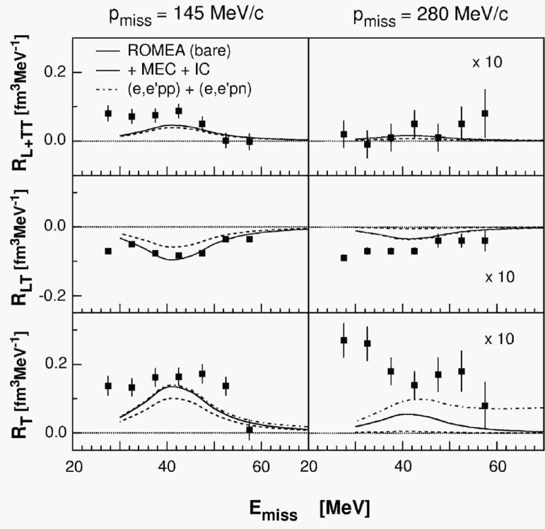
Figure 22: Data from this work together with romea calculations by the Ghent Group for the $E_{\rm miss}$-dependence of the $R_{L+TT}$, $R_{LT}$, and $R_{T}$ effective response functions. Uncertainites are statistical (see Tables LABEL:table:contrlttrt, LABEL:table:contrlt, and LABEL:table:contrlrt for the associated systematic uncertainties). Also shown is the $(e,e^{\prime}pN)$ contribution.

At $p_{\rm miss}$ = 280 MeV/$c$, the bare calculation does not reproduce the $E_{\rm miss}$-dependence of any of the measured effective response functions. The inclusion of MEC and IC in the calculation substantially increases the magnitude of all three calculated response functions, and thus improves the agreement between data and calculation. The measured $R_{L+TT}$ (which is dominated by $R_{L}$) is consistent with both the calculation and with zero. The measured $R_{LT}$ is about twice the magnitude of the calculation. Since the measured $R_{LT}$ is nonzero over the entire $E_{\rm miss}$ range, the measured $R_{L}$ must also be nonzero. The measured $R_{T}$ is significantly larger than both the calculations and nonzero out to at least $E_{\rm miss}$ $\approx$ 60 MeV. The fact that the measured $R_{T}$ is much larger than the measured $R_{L}$ indicates the cross section is largely due to transverse two-body currents. And finally, it is clear that $(e,e^{\prime}pN)$ accounts for a fraction of the measured transverse strength which increases dramatically with increasing $p_{\rm miss}$.

Fig. 23 shows the calculations by the Ghent Group Ryckebusch and Debruyne (2002) of the contribution to the differential ¹⁶O$(e,e^{\prime}p)$ cross section from two-nucleon knockout as a function of $E_{\rm miss}$ and $\theta_{p}$ for $E_{\rm beam}$ = 2.442 GeV. The upper-left panel shows the contribution of central correlations. The upper-right panel shows the combined contribution of central and tensor correlations. Tensor correlations are anticipated to dominate central correlations over the ranges of $E_{\rm miss}$ and $p_{\rm miss}$ investigated in this work. The lower-left panel shows the combined contribution of central and tensor correlations (two-nucleon correlations) together with MEC and IC (two-body currents). Two-body currents are anticipated to dominate two-nucleon correlations over the ranges of $E_{\rm miss}$ and $p_{\rm miss}$ investigated in this work. For convenience, the variation of $p_{\rm miss}$ with $E_{\rm miss}$ and $\theta_{p}$ is shown in the bottom-right panel.

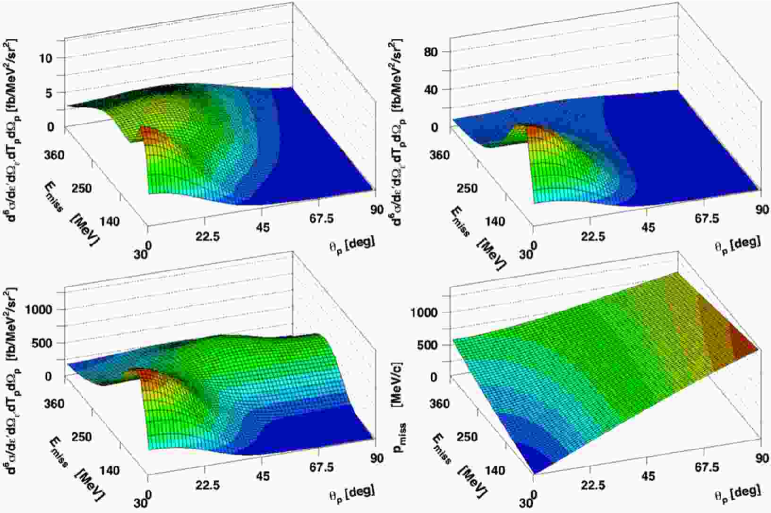
Figure 23: (Color online) Calculations by the Ghent Group of the contribution to the differential ¹⁶O$(e,e^{\prime}p)$ cross section from two-nucleon knockout as a function of $E_{\rm miss}$ and $\theta_{p}$ for $E_{\rm beam}$ = 2.442 GeV. The upper-left panel shows the contribution of central correlations. The upper-right panel shows the combined contribution of central and tensor correlations. The lower-left panel shows the combined contribution of central and tensor correlations (two-nucleon correlations) together with MEC and IC (two-body currents). The relationship between the various kinematic quantities is shown in the bottom-right panel.

VI Kinematic consistency of $\bm{1p}$-shell normalization factors

There has been longstanding discussion regarding the reliability of the spectroscopic factors determined for discrete states from single-nucleon electromagnetic knockout. Recently, there has been speculation that these factors might appear to increase with $Q^{2}$ as a quasiparticle state is probed with finer resolution. In this Section, Kelly Kelly (2002) has used the rdwia to analyze the normalization factors fitted to the available ¹⁶O$(e,e^{\prime}p)$ data for the $1p_{1/2}$- and $1p_{3/2}$-states obtained in the experiments summarized in Table 9. If the rdwia model is accurate, these factors should be independent of the experimental kinematics.

Table 9: A summary of the kinematic conditions for the data examined in the ¹⁶O$(e,e^{\prime}p)$ consistency study.

			$T_{p}$	$Q^{2}$
label	authors	kinematics	(MeV)	(GeV/$c$)2	$x$	$2s_{1/2}1d_{5/2}$-doublet	data
a	Leuschner et al. Leuschner et al. (1994)	parallel	96	varied	varied	resolved	reduced $\sigma$
b	Spaltro et al. Spaltro et al. (1993)	perpendicular	84	0.20	1.07	resolved	differential $\sigma$
c	Chinitz et al. Chinitz et al. (1991)	perpendicular	160	0.30	0.91	computed	differential $\sigma$
d	this work	perpendicular	427	0.80	0.96	computed	differential $\sigma$
e	Bernheim et al. Bernheim et al. (1982)	perpendicular	100	0.19	0.90	computed	reduced $\sigma$
f	Blomqvist1 et al. Blomqvist et al. (1995a)	parallel	92	0.08	0.30 - 0.50	resolved	reduced $\sigma$
g	Blomqvist2 et al. Blomqvist et al. (1995a)	highly varied	215	0.04 - 0.26	0.07 - 0.70	resolved	reduced $\sigma$

VI.1 RDWIA analysis of the available ¹⁶O$\bm{(e,e^{\prime}p)}$ data

The rdwia calculations used in this procedure employed the $\bar{\Gamma}_{2}$ off-shell single-nucleon current operator with the mmd form factors of Mergell et al. Mergell et al. (1996) in the Coulomb gauge. The partial-wave expansions were performed using the second-order Dirac equation, including spinor distortion. Nucleon distortion was evaluated using the edai-o and edad1 optical potentials, and electron distortion was evaluated in the $q_{\rm eff}$ Approximation. No attempt to directly fit the overlap functions to the knockout data has been made here. Instead, the recently developed wave functions hs, nlsh, and nlsh-p (recall Fig. 11) were again tested, this time to see if they could satisfactorily reproduce the experimental $p_{\rm miss}$ distributions independently of $Q^{2}$.

The results are expressed in terms of normalization factors which compare a rdwia calculation for a fully occupied subshell with experimental data and are presented in Table 10. These factors were obtained by least-squares fitting to the data in the range $p_{\rm miss}$ $<$ 200 MeV/$c$ where the rdwia should be most reliable. When experimentally unresolved, the contamination of the $1p_{3/2}$-state by the $1d_{5/2}$$2s_{1/2}$-doublet was included by the incoherent summation of the parametrizations of Leuschner et al. as previously described.

Table 10: Normalization factors deduced for the data sets presented in Table 9 for $p_{\rm miss}$ $<$ 200 MeV/$c$. The first term in each column is for the $1p_{1/2}$-state, while the second term is for the $1p_{3/2}$-state.

	edai-o												edad1
	hs				nlsh				nlsh-p				hs				nlsh				nlsh-p
	$S_{\alpha}$		$\chi^{2}$		$S_{\alpha}$		$\chi^{2}$		$S_{\alpha}$		$\chi^{2}$		$S_{\alpha}$		$\chi^{2}$		$S_{\alpha}$		$\chi^{2}$		$S_{\alpha}$		$\chi^{2}$
a	0.55	0.46	0.9	4.2	0.60	0.47	2.5	6.0	0.53	0.41	1.0	1.5	0.60	0.55	0.8	2.4	0.66	0.56	2.3	3.7	0.57	0.48	0.8	1.4
b	0.61	0.66	2.7	6.3	0.65	0.68	5.4	8.0	0.58	0.58	2.3	3.6	0.71	0.75	2.3	5.1	0.77	0.77	4.2	6.4	0.68	0.65	2.2	4.1
c	0.54	0.56	8.7	17.9	0.60	0.58	24.8	25.3	0.51	0.47	9.0	15.0	0.59	0.61	8.0	18.2	0.66	0.63	16.7	22.1	0.56	0.50	7.2	23.8
d	0.62	0.63	30.8	4.7	0.70	0.65	0.5	6.7	0.59	0.52	19.6	15.3	0.62	0.63	32.5	2.4	0.70	0.66	1.2	3.9	0.60	0.53	20.0	14.4
e	0.43	0.46	1.0	1.9	0.48	0.47	2.2	2.4	0.42	0.40	1.0	1.1	0.48	0.52	1.0	1.5	0.54	0.54	1.5	1.9	0.47	0.45	1.0	1.3
f	0.53	0.41	3.0	4.2	0.54	0.42	5.0	5.8	0.51	0.38	2.7	1.9	0.57	0.50	3.2	3.7	0.59	0.51	5.8	5.0	0.54	0.46	2.7	2.1
g	0.42	0.37	2.0	1.4	0.44	0.37	4.7	2.0	0.40	0.33	2.5	5.9	0.42	0.40	1.8	1.9	0.44	0.41	6.6	2.8	0.40	0.36	1.9	5.4

The data sets demonstrated a slight preference for the edad1 optical potential over the edai-o optical potential. This was concluded based on the quality of the fits and the more consistent nature of the extracted normalization factors for low $Q^{2}$. None of the variations considered in Table 10 (nor any of those considered in Table 7 for that matter) were able to reproduce the $1p_{3/2}$-state for data set (b) in the range $50<p_{\rm miss}<120$ MeV/$c$. This problem is also responsible for the discrepancy seen in Fig. 1 for $R_{LT}$ at $Q^{2}=0.2$ (GeV/$c$)², and has not yet been explained satisfactorily.

Unfortunately, none of the selected wave functions provided an optimal description of the experimental $p_{\rm miss}$ distributions independent of $Q^{2}$. Fig. 24 shows a sample set of fits to the various ¹⁶O$(e,e^{\prime}p)$ data sets based on the hs bound-nucleon wave function and the edad1 optical potential.

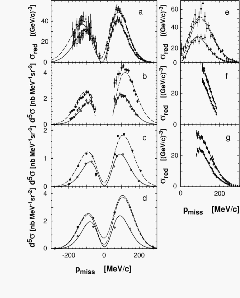
Figure 24: Fits to various ¹⁶O$(e,e^{\prime}p)$ data sets based on the hs bound-nucleon wave function and the edad1 optical potential. See Table 9 for the key to the data-set labels. Open points and solid lines pertain to the $1p_{1/2}$-state, while solid points and dashed lines pertain to the $1p_{3/2}$-state. The dashed-dotted lines include the contributions of the positive parity $2s_{1/2}1d_{5/2}$-doublet to the $1p_{3/2}$-state. Panel (d) shows the data from this work.

From a $\chi^{2}$ perspective, it is clear that nlsh offered the best description of the data at $Q^{2}=0.8$ (GeV/$c$)², but that most of the lower $Q^{2}$ data are best described by either nlsh-p or nlsh; in fact, hs may be the best compromise currently available. Data set (g) from Mainz suggested a substantially different normalization.

An estimate of the uncertainty in the normalization factors due to variations of the bound-nucleon wave function was made by comparing nlsh/hs and nlsh-p/hs normalization-factor ratios for each state holding the optical potential and other model input constant. For the lowest-lying $1p_{1/2}$- and $1p_{3/2}$-states and averaged over all data sets, nlsh/hs ratios of 1.08 and 1.02 were obtained. Similarly, nlsh-p/hs ratios of 0.96 and 0.87 were obtained. These ratios are qualitatively consistent with the behavior of the data and the calculations near the peaks of the momentum distributions shown in Fig. 11. Therefore, a cautious estimate of the uncertainty due to the bound-nucleon wave function is of order $\pm 10\%$. Further, by changing the optical potentials between edai-o and edad1 and holding the bound-nucleon wave function and other model input constant, edai-o/edad1 normalization-factor ratios for a given data set with $Q^{2}<0.4$ (GeV/$c$)² averaged to about 0.90. This ratio became 0.98 at $Q^{2}=0.8$ (GeV/$c$)², where the attenuation in the potentials is practically identical. Therefore, the uncertainty due to variations of the optical potential is at least $\pm 5\%$ and would probably be larger if the sample of ‘reasonable’ potentials were expanded.

The information presented in Table 7 suggests that there would be similar uncertainties in the normalization factors for the $Q^{2}=0.8$ (GeV/$c$)² data arising from Gordon and gauge ambiguities in the single-nucleon current operator. Note that values of $S_{\alpha}$ for the same model are generally larger in Table 7 than in Table 10 because the former summarizes a study of the entire $p_{\rm miss}$ range while the latter is limited to $p_{\rm miss}$ $<$ 200 MeV/$c$, where the reaction model is likely to be most accurate. Data for larger $p_{\rm miss}$ also tend to have a higher $\chi^{2}$. These problems for large $p_{\rm miss}$ may arise from inaccuracies in the bound-nucleon wave functions above the Fermi momentum, neglecting two-body currents, neglecting channel coupling in the final state, or density-dependence in the form factors, to name a few. Therefore, a realistic estimate of the model dependence of the normalization factors for $(e,e^{\prime}p)$ reactions should not be less than $\pm 15\%$. This estimated precision is consistent with that suggested in Ref. Kelly (1996) – although the relativistic model improves our description of $A_{LT}$, recoil polarization, and other normalization-independent features of the reaction, the model dependencies that affect the normalization uncertainty are not significantly improved. Assuming that the reaction model is most reliable at large $Q^{2}$ and modest $p_{\rm miss}$, the six $1p_{1/2}$- and $1p_{3/2}$-state normalization factors for data set (d) in Table 10 (this work) were averaged to conclude that the normalization factors for the lowest $1p_{1/2}$- and $1p_{3/2}$-states in ¹⁵N are approximately 0.63(9) and 0.60(9).

As previously mentioned, Leuschner et al. identified two additional $1p_{3/2}$-states with excitation energies between 9 and 13 MeV that together carry approximately $11\%$ of the strength of the lowest-energy fragment. However, those states were not resolved by the present experiment. If the assumption is made that the same ratio applies at $Q^{2}\approx 0.8$ (GeV/$c$)², then the total $1p_{3/2}$ strength below 15 MeV excitation is estimated to be approximately $67\%$ of full occupancy, and the total $1p$-shell spectroscopic strength below 15 MeV represents $3.9\pm 0.6$ protons or about $65\%$ of full occupancy. This result remains $10-20\%$ below predictions from recent calculations of the hole spectral function by Barbieri and Dickhoff Barbieri and Dickhoff (2002), but no experimental estimate for the additional $p$-shell strength that might lurk beneath the continuum is available.

To obtain more precise normalization factors, it would be necessary to apply a relativistic analysis to data in quasiperpendicular kinematics for several values of $Q^{2}$ larger than about 0.5 (GeV/$c$)² and with sufficient coverage of the $p_{\rm miss}$ distribution to fit the wave function, requiring that the bound-nucleon wave function be independent of $Q^{2}$. Although such data do not yet exist for ¹⁶O, the recently completed experiment in Hall A at Jefferson Lab will provide substantially more data points for the critical $p_{\rm miss}$ $<$ 200 MeV/$c$ region for $Q^{2}=$ 0.9 (GeV/$c$)².

VI.2 $\bm{Q^{2}}$-dependence of normalization factors

Lapikás et al. Lapikás et al. (2000) have performed a similar type of analysis of the $Q^{2}$-dependence of the normalization factors for the ¹²C$(e,e^{\prime}p)$ reaction. In their work, several data sets with $Q^{2}<0.3$ (GeV/$c$)² were analyzed using a nonrelativistic dwia model. For each data set, a normalization factor and the radius parameter for a Woods-Saxon binding potential were fitted to the reduced cross section for discrete states, and the potential depths were adjusted to fit the separation energies. Consistent normalization factors were obtained for all data sets save those measured by Blomqvist et al. at Mainz Blomqvist et al. (1995b). A new experiment was thus performed at NIKHEF duplicating the Mainz kinematics. The new results were also consistent with all data sets save those from Mainz. Lapikás et al. thus concluded that the Mainz data were normalized incorrectly. Recall that similar doubts regarding the normalization of the companion ¹⁶O$(e,e^{\prime}p)$ experiment Blomqvist et al. (1995a) at Mainz had been expressed earlier by Kelly Kelly (1997), but independent data duplicating the measurement are unfortunately not available. After excluding the Mainz data, Lapikás et al. determined that the summed $1p$-shell strength for ¹²C could in fact be deduced from data for $Q^{2}<0.3$ (GeV/$c$)² with an uncertainty of $\pm 3\%$. However, they did not consider the effects of variations of the optical model or several other uncertain aspects of the reaction model. As discussed previously, a more realistic estimate of the relative uncertainty in the normalization factors must be closer to $\pm 15\%$ due to the inevitable model dependence of the dwia. Furthermore, it is possible that variation of the Woods-Saxon radius might affect the resulting normalization factors. If the overlap function is an intrinsic property of the nuclear wave function, it should not depend upon $Q^{2}$. Further, it should be possible to fit a common radius to all data simultaneously; if not, the accuracy of the reaction model must be questioned. And of course, it has been demonstrated in recent years that a relativistic dwia model is preferable to a nonrelativistic approach.

Lapikás et al. also used the bound-nucleon wave functions and normalization factors obtained from their nonrelativistic analysis at low $Q^{2}$ to analyze the transparency of ¹²C for $Q^{2}$ up to 7 (GeV/$c$)² and the summed $1p$- and $1s$-shell spectroscopic amplitude. They found the summed spectroscopic strength was approximately constant at 0.58 for $Q^{2}\leq 0.6$ (GeV/$c$)², but rose for larger $Q^{2}$ and appeared to approach the Independent-Particle Model limit of unity somewhere near $Q^{2}\approx 10$ (GeV/$c$)². They speculated that the apparent $Q^{2}$-dependence of this spectroscopic strength might be related to the resolution at which a quasiparticle is probed, with long-range correlations that deplete the single-particle strength becoming less important at higher $Q^{2}$ and finer resolution. A subsequent analysis by Frankfurt et al. using Glauber calculations for heavier targets Frankfurt et al. (2001) supports this interpretation.

Little evidence is seen here for a systematic dependence in the normalization factors upon either $T_{p}$ or $Q^{2}$ for the lowest $1p$-states of ¹⁶O for the data that are presently available. Unfortunately, these data do not reach high enough $Q^{2}$ to address the resolution hypothesis. Furthermore, the normalization factors for two of the data sets appear to be anomalously low. A normalization problem might not be too surprising for data set (e) because it comes from one of the earliest experiments on this reaction, but data set (g) comes from a fairly recent experiment at Mainz and uses an ejectile energy large enough for the reaction model to be reliable. As discussed above for the case of ¹²C, it is likely that data set (g) also has a normalization error . If these two data sets are disregarded, the remaining low $Q^{2}$ data are consistent with the normalization factors deduced from the current $Q^{2}=0.8$ (GeV/$c$)² data.

VII Summary and Conclusions

The ¹⁶O$(e,e^{\prime}p)$ reaction in QE, constant $(q,\omega)$ kinematics at $Q^{2}$ $\approx$ 0.8 (GeV/$c$)², $q\approx$ 1 GeV/$c$, and $\omega\approx$ 445 MeV was studied for 0 $<$ $E_{\rm miss}$ $<$ 120 MeV and 0 $<$ $p_{\rm miss}$ $<$ 350 MeV/$c$. Five-fold differential cross-section data for the removal of protons from the $1p$-shell were obtained for 0 $<$ $p_{\rm miss}$ $<$ 350 MeV/$c$. Six-fold differential cross-section data for 0 $<$ $E_{\rm miss}$ $<$ 120 MeV were obtained for 0 $<$ $p_{\rm miss}$ $<$ 340 MeV/$c$. These results were used to extract the $A_{LT}$ asymmetry and the $R_{L}$, $R_{T}$, $R_{L+TT}$, and $R_{LT}$ effective response functions over a large range of $E_{\rm miss}$ and $p_{\rm miss}$.

The data were interpreted in subsets corresponding to the 1$p$-shell and the 1$s_{1/2}$-state and continuum, respectively. 1$p$-shell data were interpreted within three fully relativistic frameworks for single-particle knockout which do not include any two-body currents: rdwia, romea, and rmsga. Two-body current contributions to the romea and rmsga calculations for the 1$p$-shell stemming from MEC and IC were also considered. The 1$s_{1/2}$-state and continuum data were considered within the identical romea framework both before and after two-body current contributions due MEC and IC were included. $(e,e^{\prime}pN)$ contributions to these data were also examined.

Overall, the rdwia calculations provided by far the best description of the 1$p$-shell data. Dynamic effects due to the inclusion of the lower components of the Dirac spinors in these calculations were necessary to self-consistently reproduce the $1p$-shell cross-section data, the $A_{LT}$ asymmetry, and the $R_{LT}$ effective response function over the entire measured range of $p_{\rm miss}$. Within the rdwia framework, the four most important ingredients were the inclusion of both bound-nucleon and ejectile spinor distortion, the choice of current operator, the choice of bound-nucleon wave function, and the choice of optical potential. Inclusion of the spinor distortion resulted in a diffractive change in slope in $A_{LT}$ at $p_{\rm miss}$ $\approx$ 300 MeV/$c$ which agreed nicely with the data. A different choice of current operator either damped out or magnified this change in slope. A different choice of bound-nucleon wave function changed the $p_{\rm miss}$-location of the change in slope, but preserved the magnitude. A different choice of optical potential changed the magnitude of the change in slope but preserved the $p_{\rm miss}$-location.

As anticipated, since $p_{p}$ $\approx$ 1 GeV/$c$, the romea calculations provided a reasonable description of the 1$p$-shell data. For this energy range, optical models generally provide an overall better description of proton elastic scattering than does the Glauber model. This is in part due to important medium modifications of the $NN$ interaction from Pauli blocking and spinor distortion. Surprisingly, the unfactorized ‘out-of-the-box’ rmsga calculation provided a fairly good description of the 1$p$-shell data already at this relatively low proton momentum. Adding the contributions of two-body currents due to MEC and IC to the descriptions of the 1$p$-shell data provided by the bare romea and rmsga calculations did not improve the agreement.

The rdwia calculation with single-nucleon currents was used to fit normalization factors to the data from this experiment and from several other experiments at lower $Q^{2}$. Ignoring two experiments which appear to have normalization problems, normalization factors of 0.63(9) and 0.60(9) were obtained for the lowest $1p_{1/2}$- and $1p_{3/2}$-states with no significant dependence upon $Q^{2}$ or $T_{p}$. The estimated uncertainties account for variations due to the choice of bound-nucleon wave functions, optical potentials, and other aspects of the model. After accounting for other known but unresolved $1p_{3/2}$-states, the total $1p$-shell spectroscopic strength below about 15 MeV excitation is estimated to be about $0.65\pm 0.10$ relative to full occupancy.

For 25 $<$ $E_{\rm miss}$ $<$ 50 MeV and $p_{\rm miss}$ $\leq$ 145 MeV/$c$, the reaction was dominated by the knockout of $1s_{1/2}$-state protons and the cross section and effective response functions were reasonably well-described by bare romea calculations which did not consider the contributions of two-body currents due to MEC and IC. However, as $p_{\rm miss}$ increased beyond 145 MeV/$c$, the single-particle aspect of the reaction diminished. Cross-section data and response functions were no longer peaked at $E_{\rm miss}$ $\approx$ 40 MeV, nor did they exhibit the Lorentzian $s$-shell shape. Already at $p_{\rm miss}$ $=$ 280 MeV/$c$, the same bare romea calculations that did well describing the data for $p_{\rm miss}$ $<$ 145 MeV/$c$ underestimated the cross-section data by more than an order of magnitude. Including the contributions of two-body currents due to MEC and IC improved the agreement for $E_{\rm miss}$ $<$ 50 MeV, but the calculations still dramatically underpredict the data.

For 25 $<$ $E_{\rm miss}$ $<$ 120 MeV and $p_{\rm miss}$ $\geq$ 280 MeV/$c$, the cross-section data were almost constant as a function of both $p_{\rm miss}$ and $E_{\rm miss}$. Here, the single-particle aspect of the $1s_{1/2}$-state contributed $<$10% to the cross section. Two-nucleon $(e,e^{\prime}pN)$ calculations accounted for only about 50% of the magnitude of the cross-section data, but reproduced the shape well. The model, which explained the shape, transverse nature, and 50% of the measured cross section, suggested that the contributions of the two-nucleon currents due to MEC and IC are much larger than those of the two-nucleon correlations. The magnitude of the measured cross section that remains unaccounted for suggests additional currents and processes play an equally important role.

Appendix A Quasielastic results

A.1 Cross-section data

The cross-section data are presented in this section. Note that the data sets obtained for $\theta_{pq}$ $=$ 0^∘ presented in Tables LABEL:table:pshellpararesults, LABEL:table:0843cont000deg, LABEL:table:1643cont000deg, and LABEL:table:2442cont000deg do not truly represent parallel kinematics even though the HRS_h was aligned along $\bm{q}$. Since $\bm{{p}_{p}}$ and $\bm{q}$ had about the same magnitude, $\bm{{p}_{\rm miss}}$ arose from the slight angles between them, not from differences in their magnitudes. However, since the distribution of $\bm{{p}_{\rm miss}}$ was symmetrical about $\bm{q}$, the conditions of parallel kinematics were closely approximated.

A.1.1 $1p$-shell

Cross-section data for QE proton knockout from the $1p$-shell of ¹⁶O are presented in Tables LABEL:table:pshellpararesults and LABEL:table:pshellperpresults.

Table 11: Measured cross-section data for QE proton knockout from the $1p$-shell of ¹⁶O for $<T_{p}>$ = 427 MeV. The $p_{\rm miss}$ bins were 20 MeV/$c$ wide. Cuts were applied to remove the radiative tail from ¹H$(e,ep)$ such that $<p_{\rm miss}>$ = 52.5 MeV/$c$ in each case.

		$1p_{1/2}$-state				$1p_{3/2}$-state
$E_{\rm beam}$	$\theta_{pq}$	$<Q^{2}>$	$<\omega>$	$d^{5}\sigma/d\omega d\Omega_{e}d\Omega_{p}$	(sys)	$<Q^{2}>$	$<\omega>$	$d^{5}\sigma/d\omega d\Omega_{e}d\Omega_{p}$	(sys)
(GeV)	(∘)	(GeV/$c$)2	(MeV)	(nb/MeV/sr2)	(%)	(GeV/$c$)2	(MeV)	(nb/MeV/sr2)	(%)
0.843	0.0	0.810	436.0	0.0922 $\pm$ 0.0118	5.4	0.810	436.0	0.1143 $\pm$ 0.0115	5.4
1.643	0.0	0.820	421.5	0.5827 $\pm$ 0.0486	5.5	0.820	421.5	0.7418 $\pm$ 0.0514	5.4
2.442	0.0	0.815	423.0	1.5030 $\pm$ 0.1380	5.5	0.815	423.0	1.8540 $\pm$ 0.1500	5.5

Table 12: Measured cross-section data for QE proton knockout from the $1p$-shell of ¹⁶O for $<Q^{2}>$ $=$ 0.800 (GeV/$c$)², $<\omega>$ = 436 MeV, and $<T_{p}>$ = 427 MeV. The $p_{\rm miss}$ bins were 20 MeV/$c$ wide.

		$1p_{1/2}$-state			$1p_{3/2}$-state
$E_{\rm beam}$	$\theta_{pq}$	$<p_{\rm miss}>$	$d^{5}\sigma/d\omega d\Omega_{e}d\Omega_{p}$	(sys)	$<p_{\rm miss}>$	$d^{5}\sigma/d\omega d\Omega_{e}d\Omega_{p}$	(sys)
(GeV)	(∘)	(MeV/$c$)	(nb/MeV/sr2)	(%)	(MeV/$c$)	(nb/MeV/sr2)	(%)
0.843	8.0	150.0	0.0789 $\pm$ 0.0057	5.6	150.0	0.1467 $\pm$ 0.0076	5.5
	16.0	275.0	0.0011 $\pm$ 0.0003	6.1	275.0	0.0058 $\pm$ 0.0006	7.2
1.643	-8.0	-148.0	0.2950 $\pm$ 0.0320	5.5	-146.0	0.5160 $\pm$ 0.0370	5.5
	8.0	148.0	0.5250 $\pm$ 0.0310	5.5	146.0	1.0390 $\pm$ 0.0360	5.4
2.442	-20.0	-355.0	0.0023 $\pm$ 0.0011	5.5	-355.0	0.0054 $\pm$ 0.0011	5.4
	-16.0	-279.0	0.0143 $\pm$ 0.0029	5.7	-275.0	0.0288 $\pm$ 0.0051	6.1
	-8.0	-149.0	0.9060 $\pm$ 0.0260	5.5	-149.0	1.5740 $\pm$ 0.0374	5.5
	-2.5	-60.0	1.5981 $\pm$ 0.0456	5.4	-60.0	2.2360 $\pm$ 0.0540	5.5
	2.5	60.0	1.5380 $\pm$ 0.0513	5.4	60.0	2.6210 $\pm$ 0.0650	5.5
	8.0	149.0	1.4605 $\pm$ 0.0261	5.5	149.0	2.9950 $\pm$ 0.0374	5.5
	16.0	279.0	0.0303 $\pm$ 0.0029	5.7	276.0	0.1672 $\pm$ 0.0051	6.2
	20.0	330.0	0.0057 $\pm$ 0.0005	5.6	330.0	0.0214 $\pm$ 0.0008	5.5

A.1.2 Higher missing energies

Cross-section data together with statistical uncertainties for QE proton knockout from ¹⁶O for $E_{\rm miss}>$ 20 MeV are presented in Tables LABEL:table:0843cont000deg – LABEL:table:2442cont020deg.

Table 13: Measured cross-section data for QE proton knockout from ¹⁶O for $E_{\rm beam}=$ 0.843 GeV, $\theta_{pq}=$ 0.0^∘, and $E_{\rm miss}>$ 25 MeV. The $p_{\rm miss}$ bins were 5 MeV/$c$ wide. Cuts were applied to remove the radiative tail from ¹H$(e,ep)$. There is an additional 5.8% systematic uncertainty associated with these results.

$E_{\rm miss}$	$<\omega>$	$<Q^{2}>$	$<p_{\rm miss}>$	$d^{6}\sigma/d\omega dE_{p}d\Omega_{e}d\Omega_{p}$
(MeV)	(MeV)	(GeV/$c$)2	(MeV/$c$)	(nb/MeV2/sr2)
27.5	445.2	0.796	38.7	0.0024 $\pm$ 0.0005
32.5	445.2	0.795	41.8	0.0085 $\pm$ 0.0008
37.5	445.8	0.794	45.0	0.0097 $\pm$ 0.0008
42.5	446.3	0.793	48.5	0.0113 $\pm$ 0.0009
47.5	447.7	0.790	51.3	0.0106 $\pm$ 0.0010
52.5	449.7	0.786	53.2	0.0065 $\pm$ 0.0010
57.5	451.7	0.782	55.5	0.0062 $\pm$ 0.0013

Table 14: Measured cross-section data for QE proton knockout from ¹⁶O for $E_{\rm beam}=$ 0.843 GeV, $\theta_{pq}=$ 8.0^∘, and $E_{\rm miss}>$ 25 MeV. The $p_{\rm miss}$ bins were 5 MeV/$c$ wide. There is an additional 6.0% systematic uncertainty associated with these results.

$E_{\rm miss}$	$<\omega>$	$<Q^{2}>$	$<p_{\rm miss}>$	$d^{6}\sigma/d\omega dE_{p}d\Omega_{e}d\Omega_{p}$
(MeV)	(MeV)	(GeV/$c$)2	(MeV/$c$)	(nb/MeV2/sr2)
25.5	444.9	0.796	143.3	0.0048 $\pm$ 0.0013
26.5	444.6	0.796	143.5	0.0019 $\pm$ 0.0010
27.5	445.2	0.795	143.8	0.0008 $\pm$ 0.0009
28.5	444.8	0.796	143.5	0.0041 $\pm$ 0.0011
29.5	444.6	0.796	143.9	0.0024 $\pm$ 0.0010
30.5	444.7	0.796	143.9	0.0022 $\pm$ 0.0009
31.5	444.9	0.796	144.2	0.0022 $\pm$ 0.0009
32.5	444.8	0.796	144.0	0.0041 $\pm$ 0.0010
33.5	445.0	0.795	144.6	0.0023 $\pm$ 0.0009
34.5	445.0	0.795	144.5	0.0013 $\pm$ 0.0008
35.5	444.9	0.796	144.7	0.0031 $\pm$ 0.0009
36.5	445.0	0.796	145.0	0.0018 $\pm$ 0.0008
37.5	445.1	0.796	145.1	0.0042 $\pm$ 0.0010
38.5	444.9	0.796	145.9	0.0013 $\pm$ 0.0008
39.5	444.9	0.796	145.6	0.0038 $\pm$ 0.0010
40.5	445.0	0.796	146.2	0.0027 $\pm$ 0.0009
41.5	444.9	0.796	146.2	0.0030 $\pm$ 0.0008
42.5	445.1	0.795	146.4	0.0029 $\pm$ 0.0009
43.5	445.1	0.795	147.3	0.0016 $\pm$ 0.0008
44.5	444.6	0.796	147.1	0.0020 $\pm$ 0.0008
45.5	445.4	0.795	147.6	0.0023 $\pm$ 0.0008
46.5	446.1	0.793	147.8	0.0028 $\pm$ 0.0009
47.5	446.5	0.793	148.0	0.0040 $\pm$ 0.0010
48.5	447.1	0.791	148.4	0.0016 $\pm$ 0.0009
49.5	447.5	0.790	148.5	0.0033 $\pm$ 0.0010
50.5	448.0	0.789	149.3	0.0029 $\pm$ 0.0010
51.5	448.5	0.789	149.5	0.0015 $\pm$ 0.0009
52.5	449.0	0.787	149.8	0.0013 $\pm$ 0.0007
53.5	449.4	0.786	150.0	0.0024 $\pm$ 0.0007
54.5	450.0	0.785	151.1	0.0022 $\pm$ 0.0009
55.5	450.5	0.784	151.2	0.0008 $\pm$ 0.0008
56.5	451.1	0.783	151.7	0.0019 $\pm$ 0.0010
57.5	451.6	0.782	151.7	0.0010 $\pm$ 0.0010
58.5	452.0	0.782	152.7	0.0007 $\pm$ 0.0009
59.5	452.5	0.781	152.6	0.0016 $\pm$ 0.0011

Table 15: Measured cross-section data for QE proton knockout from ¹⁶O for $E_{\rm beam}=$ 0.843 GeV, $\theta_{pq}=$ 16.0^∘, and $E_{\rm miss}>$ 25 MeV. The $p_{\rm miss}$ bins were 5 MeV/$c$ wide. There is an additional 5.9% systematic uncertainty associated with these results.

$E_{\rm miss}$	$<\omega>$	$<Q^{2}>$	$<p_{\rm miss}>$	$d^{6}\sigma/d\omega dE_{p}d\Omega_{e}d\Omega_{p}$
(MeV)	(MeV)	(GeV/$c$)2	(MeV/$c$)	(nb/MeV2/sr2)
27.5	446.0	0.795	281.6	0.0004 $\pm$ 0.0001
32.5	446.0	0.795	281.3	0.0003 $\pm$ 0.0001
37.5	445.9	0.795	281.2	0.0003 $\pm$ 0.0001
42.5	446.1	0.795	281.0	0.0002 $\pm$ 0.0001
47.5	448.1	0.790	281.8	0.0002 $\pm$ 0.0001
52.5	450.5	0.786	282.6	0.0003 $\pm$ 0.0001
57.5	452.8	0.781	283.6	0.0002 $\pm$ 0.0001

Table 16: Measured cross-section data for QE proton knockout from ¹⁶O for $E_{\rm beam}=$ 1.643 GeV, $\theta_{pq}=$ 0.0^∘, and $E_{\rm miss}$ $>$ 25 MeV. The $p_{\rm miss}$ bins were 5 MeV/$c$ wide. Cuts were applied to remove the radiative tail from ¹H$(e,ep)$. There is an additional 5.8% systematic uncertainty associated with these results.

$E_{\rm miss}$	$<\omega>$	$<Q^{2}>$	$<p_{\rm miss}>$	$d^{6}\sigma/d\omega dE_{p}d\Omega_{e}d\Omega_{p}$
(MeV)	(MeV)	(GeV/$c$)2	(MeV/$c$)	(nb/MeV2/sr2)
27.5	450.0	0.795	62.5	0.0195 $\pm$ 0.0013
32.5	450.0	0.795	62.5	0.0293 $\pm$ 0.0012
37.5	450.0	0.795	62.5	0.0483 $\pm$ 0.0013
42.5	450.0	0.795	62.5	0.0534 $\pm$ 0.0014
47.5	450.0	0.795	62.5	0.0445 $\pm$ 0.0014
52.5	450.0	0.795	65.0	0.0263 $\pm$ 0.0015
57.5	450.0	0.795	67.5	0.0132 $\pm$ 0.0021

Table 17: Measured cross-section data for QE proton knockout from ¹⁶O for $E_{\rm beam}$ $=$ 1.643 GeV, $|\theta_{pq}|=$ 8.0^∘, and $E_{\rm miss}$ $>$ 25 MeV. The $p_{\rm miss}$ bins were 5 MeV/$c$ wide. There is an additional 6.0% systematic uncertainty associated with these results.

			$\theta_{pq}=+8.0^{\circ}$		$\theta_{pq}=-8.0^{\circ}$
$E_{\rm miss}$	$<\omega>$	$<Q^{2}>$	$<p_{\rm miss}>$	$d^{6}\sigma/d\omega dE_{p}d\Omega_{e}d\Omega_{p}$	$<p_{\rm miss}>$	$d^{6}\sigma/d\omega dE_{p}d\Omega_{e}d\Omega_{p}$
(MeV)	(MeV)	(GeV/$c$)2	(MeV/$c$)	(nb/MeV2/sr2)	(MeV/$c$)	(nb/MeV2/sr2)
25.5	436.2	0.804	141.8	0.0361 $\pm$ 0.0036	153.2	0.0163 $\pm$ 0.0020
26.5	438.0	0.802	142.7	0.0231 $\pm$ 0.0031	152.2	0.0130 $\pm$ 0.0018
27.5	439.0	0.802	144.1	0.0193 $\pm$ 0.0029	151.7	0.0079 $\pm$ 0.0016
28.5	439.5	0.802	144.9	0.0138 $\pm$ 0.0026	150.5	0.0060 $\pm$ 0.0015
29.5	441.2	0.800	146.6	0.0167 $\pm$ 0.0026	149.7	0.0117 $\pm$ 0.0016
30.5	441.7	0.800	146.8	0.0209 $\pm$ 0.0027	148.8	0.0132 $\pm$ 0.0016
31.5	442.4	0.801	147.5	0.0157 $\pm$ 0.0025	147.4	0.0101 $\pm$ 0.0015
32.5	443.6	0.799	148.8	0.0201 $\pm$ 0.0026	147.2	0.0075 $\pm$ 0.0014
33.5	445.1	0.798	149.9	0.0185 $\pm$ 0.0026	146.1	0.0098 $\pm$ 0.0014
34.5	445.8	0.796	151.3	0.0171 $\pm$ 0.0025	144.6	0.0138 $\pm$ 0.0015
35.5	446.9	0.796	151.1	0.0178 $\pm$ 0.0025	144.3	0.0109 $\pm$ 0.0015
36.5	447.5	0.796	151.9	0.0226 $\pm$ 0.0026	144.0	0.0135 $\pm$ 0.0015
37.5	448.9	0.795	153.8	0.0218 $\pm$ 0.0025	142.7	0.0128 $\pm$ 0.0015
38.5	450.0	0.796	154.5	0.0245 $\pm$ 0.0027	141.7	0.0139 $\pm$ 0.0016
39.5	450.6	0.795	155.1	0.0214 $\pm$ 0.0026	140.9	0.0151 $\pm$ 0.0016
40.5	451.5	0.795	156.0	0.0242 $\pm$ 0.0027	141.1	0.0128 $\pm$ 0.0015
41.5	452.0	0.793	156.6	0.0264 $\pm$ 0.0027	139.6	0.0144 $\pm$ 0.0016
42.5	453.7	0.792	158.1	0.0171 $\pm$ 0.0025	137.9	0.0173 $\pm$ 0.0017
43.5	454.9	0.791	159.3	0.0175 $\pm$ 0.0024	137.9	0.0144 $\pm$ 0.0016
44.5	456.3	0.791	160.9	0.0202 $\pm$ 0.0025	136.6	0.0142 $\pm$ 0.0016
45.5	456.6	0.791	160.4	0.0203 $\pm$ 0.0025	135.5	0.0166 $\pm$ 0.0016
46.5	457.4	0.789	161.3	0.0136 $\pm$ 0.0022	136.3	0.0149 $\pm$ 0.0016
47.5	459.0	0.788	162.5	0.0146 $\pm$ 0.0022	134.5	0.0162 $\pm$ 0.0016
48.5	459.9	0.788	163.7	0.0170 $\pm$ 0.0023	133.7	0.0127 $\pm$ 0.0015
49.5	461.1	0.787	164.6	0.0144 $\pm$ 0.0022	132.8	0.0125 $\pm$ 0.0015
50.5	462.3	0.787	165.6	0.0157 $\pm$ 0.0023	132.5	0.0138 $\pm$ 0.0016
51.5	462.8	0.786	166.4	0.0142 $\pm$ 0.0021	131.9	0.0110 $\pm$ 0.0015
52.5	464.5	0.785	168.0	0.0079 $\pm$ 0.0019	130.2	0.0130 $\pm$ 0.0015
53.5	464.6	0.785	168.4	0.0078 $\pm$ 0.0019	130.8	0.0093 $\pm$ 0.0014
54.5	465.5	0.784	169.3	0.0073 $\pm$ 0.0018	130.1	0.0112 $\pm$ 0.0014
55.5	466.4	0.785	170.1	0.0096 $\pm$ 0.0019	129.7	0.0109 $\pm$ 0.0015
56.5	467.0	0.784	170.5	0.0094 $\pm$ 0.0019	128.3	0.0069 $\pm$ 0.0013
57.5	467.3	0.783	171.1	0.0066 $\pm$ 0.0018	128.4	0.0078 $\pm$ 0.0013
58.5	468.2	0.783	171.0	0.0062 $\pm$ 0.0018	129.5	0.0070 $\pm$ 0.0013
59.5	468.3	0.782	171.8	0.0041 $\pm$ 0.0016	127.2	0.0097 $\pm$ 0.0014
60.5	469.2	0.782	173.1	0.0100 $\pm$ 0.0019	127.8	0.0070 $\pm$ 0.0013
61.5	469.3	0.782	172.9	0.0060 $\pm$ 0.0018	127.1	0.0036 $\pm$ 0.0012
62.5	470.6	0.782	173.9	0.0051 $\pm$ 0.0018	127.3	0.0085 $\pm$ 0.0014
63.5	469.9	0.782	173.6	0.0062 $\pm$ 0.0017	126.8	0.0040 $\pm$ 0.0012
64.5	471.0	0.781	174.7	0.0071 $\pm$ 0.0019	126.9	0.0065 $\pm$ 0.0013
65.5	471.2	0.780	174.5	0.0045 $\pm$ 0.0018	125.8	0.0043 $\pm$ 0.0013
66.5	472.1	0.779	175.5	0.0077 $\pm$ 0.0019	125.9	0.0056 $\pm$ 0.0013
67.5	472.6	0.780	175.9	0.0049 $\pm$ 0.0019	125.5	0.0019 $\pm$ 0.0012
68.5	473.4	0.779	177.2	0.0061 $\pm$ 0.0019	126.1	0.0049 $\pm$ 0.0013
69.5	473.3	0.779	177.0	0.0071 $\pm$ 0.0019	124.0	0.0022 $\pm$ 0.0012
70.5	474.4	0.778	177.9	0.0020 $\pm$ 0.0017	125.2	0.0056 $\pm$ 0.0013
71.5	474.5	0.779	178.7	0.0033 $\pm$ 0.0017	124.8	0.0034 $\pm$ 0.0013
72.5	474.9	0.778	178.4	0.0052 $\pm$ 0.0018	125.2	0.0066 $\pm$ 0.0015
73.5	475.1	0.778	179.0	0.0065 $\pm$ 0.0020	125.1	0.0046 $\pm$ 0.0014
74.5	476.3	0.777	179.6	0.0027 $\pm$ 0.0018	124.4	0.0032 $\pm$ 0.0013
75.5	476.2	0.776	180.3	0.0026 $\pm$ 0.0017	124.4	0.0046 $\pm$ 0.0014
76.5	477.1	0.776	181.4	0.0061 $\pm$ 0.0021	122.3	0.0005 $\pm$ 0.0012
77.5	477.6	0.776	181.7	0.0034 $\pm$ 0.0019	124.1	0.0016 $\pm$ 0.0013
78.5	478.2	0.777	182.7	0.0056 $\pm$ 0.0021	123.8	0.0013 $\pm$ 0.0014
79.5	478.9	0.775	183.1	0.0056 $\pm$ 0.0021	123.4	0.0054 $\pm$ 0.0016
80.5	479.1	0.774	183.3	0.0059 $\pm$ 0.0023	122.9	0.0040 $\pm$ 0.0016
81.5	479.6	0.776	184.1	0.0008 $\pm$ 0.0018	122.7	0.0039 $\pm$ 0.0017
82.5	480.1	0.775	185.1	0.0007 $\pm$ 0.0018	122.8	0.0029 $\pm$ 0.0016
83.5	480.6	0.776	185.2	0.0039 $\pm$ 0.0021	121.8	0.0022 $\pm$ 0.0016
84.5	481.1	0.773	185.8	0.0058 $\pm$ 0.0025	122.8	0.0018 $\pm$ 0.0016
85.5	481.6	0.775	186.3	0.0028 $\pm$ 0.0023	122.2	0.0039 $\pm$ 0.0019
86.5	482.1	0.775	187.1	0.0065 $\pm$ 0.0027	122.9	0.0003 $\pm$ 0.0018
87.5	482.8	0.772	187.6	0.0049 $\pm$ 0.0030	123.1	0.0029 $\pm$ 0.0021

Table 18: Measured cross-section data for QE proton knockout from ¹⁶O for $E_{\rm beam}$ $=$ 2.442 GeV, $\theta_{pq}=$ 0.0^∘, and $E_{\rm miss}>$ 25 MeV. The $p_{\rm miss}$ bins were 5 MeV/$c$ wide. Cuts were applied to remove the radiative tail from ¹H$(e,ep)$. There is an additional 5.8% systematic uncertainty associated with these results.

$E_{\rm miss}$	$<\omega>$	$<Q^{2}>$	$<p_{\rm miss}>$	$d^{6}\sigma/d\omega dE_{p}d\Omega_{e}d\Omega_{p}$
(MeV)	(MeV)	(GeV/$c$)2	(MeV/$c$)	(nb/MeV2/sr2)
27.5	450.0	0.795	60.0	0.0552 $\pm$ 0.0042
32.5	450.0	0.795	60.0	0.0890 $\pm$ 0.0045
37.5	450.0	0.795	60.0	0.1387 $\pm$ 0.0050
42.5	450.0	0.795	60.0	0.1580 $\pm$ 0.0058
47.5	450.0	0.795	62.5	0.1348 $\pm$ 0.0062
52.5	450.0	0.795	65.0	0.0756 $\pm$ 0.0063
57.5	450.0	0.795	67.5	0.0402 $\pm$ 0.0084

Table 19: Measured cross-section data for QE proton knockout from ¹⁶O for $E_{\rm beam}$ $=$ 2.442 GeV, $\theta_{pq}=$ $-2.5^{\circ}$, and $E_{\rm miss}$ $>$ 25 MeV. The $p_{\rm miss}$ bins were 5 MeV/$c$ wide. There is an additional 5.9% systematic uncertainty associated with these results.

$E_{\rm miss}$	$<\omega>$	$<Q^{2}>$	$<p_{\rm miss}>$	$d^{6}\sigma/d\omega dE_{p}d\Omega_{e}d\Omega_{p}$
(MeV)	(MeV)	(GeV/$c$)2	(MeV/$c$)	(nb/MeV2/sr2)
25.5	445.0	0.823	46.5	0.0330 $\pm$ 0.0182
26.5	446.5	0.822	46.8	0.0661 $\pm$ 0.0185
27.5	449.5	0.821	46.7	0.0388 $\pm$ 0.0173
28.5	449.3	0.820	45.3	0.0590 $\pm$ 0.0176
29.5	450.4	0.823	46.2	0.0955 $\pm$ 0.0192
30.5	450.8	0.823	45.0	0.0589 $\pm$ 0.0181
31.5	451.9	0.821	45.4	0.0733 $\pm$ 0.0180
32.5	452.1	0.823	45.0	0.0810 $\pm$ 0.0179
33.5	453.3	0.822	45.6	0.0944 $\pm$ 0.0192
34.5	454.5	0.821	45.2	0.1375 $\pm$ 0.0211
35.5	455.1	0.821	46.1	0.0984 $\pm$ 0.0209
36.5	454.9	0.822	46.1	0.1950 $\pm$ 0.0227
37.5	457.3	0.821	45.6	0.1566 $\pm$ 0.0232
38.5	458.4	0.820	45.8	0.1937 $\pm$ 0.0232
39.5	458.4	0.820	46.1	0.2052 $\pm$ 0.0251
40.5	459.3	0.821	46.5	0.1841 $\pm$ 0.0236
41.5	459.9	0.819	45.8	0.2354 $\pm$ 0.0252
42.5	461.3	0.818	45.9	0.2401 $\pm$ 0.0260
43.5	462.7	0.817	45.6	0.1791 $\pm$ 0.0247
44.5	462.6	0.818	46.6	0.2049 $\pm$ 0.0245
45.5	464.0	0.816	45.9	0.1401 $\pm$ 0.0223
46.5	464.7	0.816	46.9	0.1721 $\pm$ 0.0224
47.5	467.9	0.817	45.7	0.1457 $\pm$ 0.0217
48.5	467.7	0.816	45.9	0.1323 $\pm$ 0.0211
49.5	468.2	0.815	45.8	0.1469 $\pm$ 0.0211
50.5	471.1	0.814	45.3	0.0893 $\pm$ 0.0189
51.5	471.0	0.814	45.9	0.1008 $\pm$ 0.0185
52.5	473.1	0.814	46.3	0.0866 $\pm$ 0.0175
53.5	472.1	0.813	45.8	0.1037 $\pm$ 0.0183
54.5	474.6	0.813	45.7	0.0607 $\pm$ 0.0165
55.5	474.5	0.812	45.4	0.0766 $\pm$ 0.0163
56.5	473.8	0.810	46.8	0.0617 $\pm$ 0.0155
57.5	476.5	0.810	45.8	0.0606 $\pm$ 0.0155
58.5	477.4	0.811	46.6	0.0717 $\pm$ 0.0158
59.5	479.4	0.809	45.1	0.0837 $\pm$ 0.0168
60.5	481.5	0.810	45.5	0.0298 $\pm$ 0.0140
61.5	480.8	0.807	46.2	0.0748 $\pm$ 0.0156
62.5	480.6	0.807	47.7	0.0165 $\pm$ 0.0125
63.5	480.7	0.805	47.8	0.0240 $\pm$ 0.0118
64.5	481.1	0.805	47.6	0.0135 $\pm$ 0.0109
65.5	484.1	0.805	46.5	0.0471 $\pm$ 0.0127
66.5	482.4	0.804	46.6	0.0195 $\pm$ 0.0118
67.5	485.9	0.804	47.4	0.0297 $\pm$ 0.0121
68.5	484.4	0.803	48.7	0.0491 $\pm$ 0.0134
69.5	490.6	0.802	46.5	0.0118 $\pm$ 0.0116
70.5	489.5	0.800	47.6	0.0021 $\pm$ 0.0103
71.5	490.8	0.800	48.3	0.0136 $\pm$ 0.0103
72.5	491.7	0.800	47.9	0.0306 $\pm$ 0.0118
73.5	491.6	0.799	49.2	0.0156 $\pm$ 0.0113
74.5	493.1	0.797	49.6	0.0192 $\pm$ 0.0114
75.5	494.7	0.798	49.1	0.0040 $\pm$ 0.0101
76.5	493.8	0.797	49.2	0.0144 $\pm$ 0.0111
77.5	496.0	0.795	48.7	0.0098 $\pm$ 0.0118
78.5	497.2	0.794	48.8	-0.0039 $\pm$ 0.0099
79.5	498.3	0.793	50.8	0.0103 $\pm$ 0.0124

Table 20: Measured cross-section data for QE proton knockout from ¹⁶O for $E_{\rm beam}$ $=$ 2.442 GeV, $|\theta_{pq}|$ $=$ 8.0^∘, and $E_{\rm miss}$ $>$ 25 MeV. The $p_{\rm miss}$ bins were 5 MeV/$c$ wide. There is an additional 6.0% systematic uncertainty associated with these results.

			$\theta_{pq}=+8.0^{\circ}$		$\theta_{pq}=-8.0^{\circ}$
$E_{\rm miss}$	$<\omega>$	$<Q^{2}>$	$<p_{\rm miss}>$	$d^{6}\sigma/d\omega dE_{p}d\Omega_{e}d\Omega_{p}$	$<p_{\rm miss}>$	$d^{6}\sigma/d\omega dE_{p}d\Omega_{e}d\Omega_{p}$
(MeV)	(MeV)	(GeV/$c$)2	(MeV/$c$)	(nb/MeV2/sr2)	(MeV/$c$)	(nb/MeV2/sr2)
25.5	438.1	0.793	150.0	0.0595 $\pm$ 0.0058	160.0	0.0174 $\pm$ 0.0030
26.5	439.6	0.791	152.5	0.0310 $\pm$ 0.0051	160.0	0.0165 $\pm$ 0.0027
27.5	440.5	0.791	155.0	0.0371 $\pm$ 0.0049	155.2	0.0190 $\pm$ 0.0026
28.5	441.7	0.789	155.0	0.0474 $\pm$ 0.0050	157.9	0.0249 $\pm$ 0.0027
29.5	442.3	0.789	152.8	0.0566 $\pm$ 0.0051	155.2	0.0306 $\pm$ 0.0028
30.5	443.4	0.788	155.0	0.0412 $\pm$ 0.0048	157.5	0.0221 $\pm$ 0.0027
31.5	444.4	0.792	157.5	0.0492 $\pm$ 0.0048	155.0	0.0318 $\pm$ 0.0028
32.5	446.6	0.788	160.0	0.0545 $\pm$ 0.0048	155.0	0.0247 $\pm$ 0.0027
33.5	447.8	0.789	160.0	0.0450 $\pm$ 0.0047	155.0	0.0289 $\pm$ 0.0027
34.5	448.0	0.788	160.0	0.0498 $\pm$ 0.0047	152.7	0.0291 $\pm$ 0.0027
35.5	449.5	0.784	160.0	0.0625 $\pm$ 0.0049	150.0	0.0294 $\pm$ 0.0027
36.5	449.1	0.784	160.0	0.0609 $\pm$ 0.0049	150.0	0.0309 $\pm$ 0.0027
37.5	452.1	0.786	162.5	0.0443 $\pm$ 0.0046	147.5	0.0357 $\pm$ 0.0028
38.5	452.7	0.788	162.5	0.0521 $\pm$ 0.0046	150.0	0.0413 $\pm$ 0.0029
39.5	453.7	0.785	165.0	0.0459 $\pm$ 0.0045	147.9	0.0336 $\pm$ 0.0028
40.5	454.1	0.783	165.0	0.0537 $\pm$ 0.0046	145.2	0.0359 $\pm$ 0.0028
41.5	454.6	0.784	165.0	0.0416 $\pm$ 0.0044	147.5	0.0368 $\pm$ 0.0028
42.5	456.7	0.783	165.0	0.0456 $\pm$ 0.0044	147.5	0.0431 $\pm$ 0.0030
43.5	456.9	0.782	167.8	0.0421 $\pm$ 0.0043	147.5	0.0350 $\pm$ 0.0028
44.5	457.3	0.780	170.0	0.0392 $\pm$ 0.0042	145.0	0.0382 $\pm$ 0.0028
45.5	457.8	0.784	167.5	0.0462 $\pm$ 0.0043	142.7	0.0335 $\pm$ 0.0028
46.5	458.3	0.781	170.0	0.0387 $\pm$ 0.0042	145.0	0.0330 $\pm$ 0.0028
47.5	459.8	0.779	172.5	0.0408 $\pm$ 0.0042	145.2	0.0326 $\pm$ 0.0027
48.5	460.4	0.782	170.0	0.0317 $\pm$ 0.0040	142.7	0.0331 $\pm$ 0.0027
49.5	461.6	0.783	175.0	0.0287 $\pm$ 0.0039	143.0	0.0217 $\pm$ 0.0025
50.5	463.6	0.779	172.8	0.0249 $\pm$ 0.0037	143.0	0.0274 $\pm$ 0.0026
51.5	463.5	0.780	175.0	0.0268 $\pm$ 0.0037	142.5	0.0257 $\pm$ 0.0025
52.5	463.1	0.784	172.8	0.0208 $\pm$ 0.0035	145.0	0.0222 $\pm$ 0.0025
53.5	465.2	0.778	172.5	0.0170 $\pm$ 0.0034	145.4	0.0191 $\pm$ 0.0024
54.5	466.2	0.779	175.0	0.0249 $\pm$ 0.0035	145.0	0.0214 $\pm$ 0.0024
55.5	468.5	0.782	180.0	0.0147 $\pm$ 0.0032	145.0	0.0175 $\pm$ 0.0023
56.5	468.6	0.778	180.0	0.0211 $\pm$ 0.0034	143.4	0.0160 $\pm$ 0.0022
57.5	469.3	0.779	177.5	0.0144 $\pm$ 0.0032	140.5	0.0181 $\pm$ 0.0022
58.5	471.3	0.774	182.5	0.0131 $\pm$ 0.0031	142.5	0.0149 $\pm$ 0.0022
59.5	472.3	0.778	180.0	0.0147 $\pm$ 0.0031	142.7	0.0145 $\pm$ 0.0022
60.5	472.3	0.778	177.5	0.0149 $\pm$ 0.0031	145.0	0.0143 $\pm$ 0.0021
61.5	474.9	0.780	185.0	0.0057 $\pm$ 0.0028	143.2	0.0131 $\pm$ 0.0021
62.5	473.8	0.781	185.0	0.0164 $\pm$ 0.0030	137.5	0.0156 $\pm$ 0.0021
63.5	475.9	0.784	187.5	0.0112 $\pm$ 0.0029	140.8	0.0087 $\pm$ 0.0020
64.5	477.0	0.783	185.0	0.0127 $\pm$ 0.0029	137.8	0.0105 $\pm$ 0.0020
65.5	477.6	0.784	185.0	0.0085 $\pm$ 0.0028	140.0	0.0081 $\pm$ 0.0019
66.5	477.2	0.777	187.5	0.0142 $\pm$ 0.0029	138.6	0.0089 $\pm$ 0.0019
67.5	477.0	0.781	190.0	0.0111 $\pm$ 0.0029	135.6	0.0086 $\pm$ 0.0019
68.5	480.2	0.780	187.5	0.0114 $\pm$ 0.0029	137.5	0.0077 $\pm$ 0.0018
69.5	480.0	0.782	187.5	0.0061 $\pm$ 0.0026	135.0	0.0089 $\pm$ 0.0019
70.5	481.1	0.778	190.0	0.0096 $\pm$ 0.0027	138.0	0.0074 $\pm$ 0.0018
71.5	481.7	0.778	192.5	0.0044 $\pm$ 0.0025	133.4	0.0030 $\pm$ 0.0016
72.5	481.7	0.781	192.5	0.0051 $\pm$ 0.0024	138.0	0.0080 $\pm$ 0.0018
73.5	482.8	0.782	192.5	0.0133 $\pm$ 0.0027	134.6	0.0058 $\pm$ 0.0018
74.5	484.8	0.781	192.8	0.0097 $\pm$ 0.0027	137.5	0.0063 $\pm$ 0.0018
75.5	485.0	0.779	197.2	0.0046 $\pm$ 0.0025	136.4	0.0057 $\pm$ 0.0017
76.5	484.6	0.773	195.0	0.0057 $\pm$ 0.0025	128.2	0.0036 $\pm$ 0.0016
77.5	485.5	0.781	192.5	0.0048 $\pm$ 0.0024	135.0	0.0030 $\pm$ 0.0016
78.5	488.2	0.781	195.3	0.0054 $\pm$ 0.0024	132.5	0.0070 $\pm$ 0.0017
79.5	488.6	0.782	197.5	0.0026 $\pm$ 0.0023	132.5	0.0033 $\pm$ 0.0016
80.5	490.3	0.785	195.3	0.0104 $\pm$ 0.0026	133.1	0.0077 $\pm$ 0.0017
81.5	489.1	0.785	197.5	0.0035 $\pm$ 0.0024	132.5	0.0048 $\pm$ 0.0017
82.5	492.5	0.782	197.8	0.0045 $\pm$ 0.0023	134.3	0.0043 $\pm$ 0.0017
83.5	492.3	0.782	197.5	0.0025 $\pm$ 0.0023	135.3	0.0027 $\pm$ 0.0016
84.5	492.6	0.778	200.0	0.0065 $\pm$ 0.0024	127.5	0.0072 $\pm$ 0.0017
85.5	495.2	0.787	200.0	0.0048 $\pm$ 0.0024	137.5	0.0024 $\pm$ 0.0016
86.5	495.6	0.790	202.5	0.0025 $\pm$ 0.0023	133.7	0.0021 $\pm$ 0.0016
87.5	498.7	0.787	200.0	0.0119 $\pm$ 0.0026	127.5	0.0021 $\pm$ 0.0016
88.5	499.6	0.785	200.0	0.0044 $\pm$ 0.0025	127.5	0.0033 $\pm$ 0.0016
89.5	497.7	0.784	202.5	0.0086 $\pm$ 0.0026	130.3	0.0008 $\pm$ 0.0016
90.5	497.8	0.781	202.5	0.0052 $\pm$ 0.0026	133.1	0.0031 $\pm$ 0.0017
91.5	499.1	0.782	202.5	0.0023 $\pm$ 0.0024	132.2	0.0029 $\pm$ 0.0018
92.5	500.8	0.789	202.5	0.0067 $\pm$ 0.0026	130.3	-0.0008 $\pm$ 0.0016
93.5	500.4	0.794	207.5	0.0060 $\pm$ 0.0026	132.8	0.0022 $\pm$ 0.0017
94.5	498.8	0.779	202.5	0.0059 $\pm$ 0.0026	128.8	-0.0003 $\pm$ 0.0017
95.5	498.8	0.775	202.5	0.0085 $\pm$ 0.0028	131.2	0.0021 $\pm$ 0.0017
96.5	499.6	0.782	205.0	0.0087 $\pm$ 0.0028	127.5	0.0049 $\pm$ 0.0019
97.5	499.2	0.790	210.0	0.0022 $\pm$ 0.0026	132.5	0.0038 $\pm$ 0.0019
98.5	501.6	0.782	205.0	0.0118 $\pm$ 0.0031	128.2	-0.0024 $\pm$ 0.0015
99.5	504.3	0.774	205.0	0.0080 $\pm$ 0.0029	125.7	0.0000 $\pm$ 0.0017
100.5	503.0	0.781	207.5	0.0031 $\pm$ 0.0027	127.5	0.0016 $\pm$ 0.0019
101.5	500.7	0.776	207.5	0.0105 $\pm$ 0.0031	126.7	0.0008 $\pm$ 0.0019
102.5	502.6	0.776	210.0	0.0021 $\pm$ 0.0028	125.4	0.0006 $\pm$ 0.0018
103.5	501.9	0.776	210.0	0.0030 $\pm$ 0.0028	130.0	-0.0013 $\pm$ 0.0017
104.5	504.8	0.780	207.5	0.0080 $\pm$ 0.0031	127.8	0.0016 $\pm$ 0.0019
105.5	503.6	0.774	210.0	0.0051 $\pm$ 0.0031	125.0	-0.0004 $\pm$ 0.0018
106.5	507.9	0.778	210.5	0.0000 $\pm$ 0.0028	129.0	-0.0027 $\pm$ 0.0016
107.5	507.1	0.784	210.0	0.0112 $\pm$ 0.0034	127.5	0.0048 $\pm$ 0.0022
108.5	509.3	0.781	212.5	0.0036 $\pm$ 0.0032	125.0	0.0033 $\pm$ 0.0023
109.5	510.0	0.781	212.5	0.0047 $\pm$ 0.0032	124.0	-0.0014 $\pm$ 0.0019
110.5	510.0	0.779	212.5	0.0020 $\pm$ 0.0031	126.1	0.0028 $\pm$ 0.0022
111.5	510.0	0.782	212.5	0.0024 $\pm$ 0.0030	122.5	-0.0007 $\pm$ 0.0022
112.5	510.0	0.779	212.5	0.0046 $\pm$ 0.0033	122.5	0.0025 $\pm$ 0.0024
113.5	510.0	0.769	216.4	0.0114 $\pm$ 0.0038	117.5	0.0029 $\pm$ 0.0025
114.5	510.0	0.778	215.0	0.0095 $\pm$ 0.0040	120.2	-0.0013 $\pm$ 0.0021
115.5	510.0	0.777	215.0	0.0048 $\pm$ 0.0037	122.5	-0.0015 $\pm$ 0.0020
116.5	510.0	0.776	215.8	0.0018 $\pm$ 0.0034	121.0	0.0005 $\pm$ 0.0021
117.5	510.0	0.774	215.0	0.0017 $\pm$ 0.0033	121.4	0.0017 $\pm$ 0.0023
118.5	510.0	0.759	217.5	0.0127 $\pm$ 0.0045	113.6	0.0016 $\pm$ 0.0024
119.5	510.0	0.777	217.5	0.0078 $\pm$ 0.0046	122.5	0.0018 $\pm$ 0.0027

Table 21: Measured cross-section data for QE proton knockout from ¹⁶O for $E_{\rm beam}$ $=$ 2.442 GeV, $|\theta_{pq}|$ $=$ 16.0^∘, and $E_{\rm miss}$ $>$ 25 MeV. The $p_{\rm miss}$ bins were 5 MeV/$c$ wide. There is an additional 5.8% systematic uncertainty associated with these results.

			$\theta_{pq}=+16.0^{\circ}$		$\theta_{pq}=-16.0^{\circ}$
$E_{\rm miss}$	$<\omega>$	$<Q^{2}>$	$<p_{\rm miss}>$	$d^{6}\sigma/d\omega dE_{p}d\Omega_{e}d\Omega_{p}$	$<p_{\rm miss}>$	$d^{6}\sigma/d\omega dE_{p}d\Omega_{e}d\Omega_{p}$
(MeV)	(MeV)	(GeV/$c$)2	(MeV/$c$)	(nb/MeV2/sr2)	(MeV/$c$)	(nb/MeV2/sr2)
25.5	439.9	0.794	268.9	0.0078 $\pm$ 0.0008	282.1	0.0095 $\pm$ 0.0020
26.5	440.0	0.788	273.8	0.0076 $\pm$ 0.0008	278.1	0.0014 $\pm$ 0.0019
27.5	443.6	0.799	274.9	0.0053 $\pm$ 0.0007	280.4	0.0078 $\pm$ 0.0020
28.5	444.8	0.788	275.8	0.0054 $\pm$ 0.0007	276.0	0.0043 $\pm$ 0.0020
29.5	447.2	0.789	277.7	0.0075 $\pm$ 0.0007	278.0	0.0053 $\pm$ 0.0021
30.5	444.0	0.799	278.9	0.0054 $\pm$ 0.0007	279.0	0.0078 $\pm$ 0.0021
31.5	451.2	0.795	277.1	0.0047 $\pm$ 0.0006	273.6	0.0068 $\pm$ 0.0020
32.5	447.8	0.797	278.6	0.0036 $\pm$ 0.0006	277.3	0.0077 $\pm$ 0.0020
33.5	449.0	0.795	280.6	0.0045 $\pm$ 0.0006	273.8	0.0015 $\pm$ 0.0019
34.5	445.9	0.787	281.2	0.0059 $\pm$ 0.0007	277.1	0.0064 $\pm$ 0.0020
35.5	451.3	0.790	281.1	0.0036 $\pm$ 0.0006	275.1	0.0049 $\pm$ 0.0021
36.5	448.8	0.785	281.3	0.0044 $\pm$ 0.0006	272.1	0.0024 $\pm$ 0.0019
37.5	451.6	0.784	282.8	0.0039 $\pm$ 0.0006	271.3	0.0041 $\pm$ 0.0019
38.5	453.3	0.779	284.2	0.0046 $\pm$ 0.0006	268.3	0.0037 $\pm$ 0.0019
39.5	452.9	0.790	284.8	0.0039 $\pm$ 0.0006	270.9	0.0059 $\pm$ 0.0019
40.5	456.0	0.789	287.8	0.0033 $\pm$ 0.0006	268.4	0.0027 $\pm$ 0.0018
41.5	452.7	0.791	287.2	0.0041 $\pm$ 0.0006	270.6	0.0057 $\pm$ 0.0019
42.5	453.2	0.795	285.1	0.0039 $\pm$ 0.0006	270.3	0.0067 $\pm$ 0.0020
43.5	455.0	0.784	288.1	0.0028 $\pm$ 0.0005	268.5	0.0057 $\pm$ 0.0019
44.5	456.2	0.795	290.3	0.0033 $\pm$ 0.0005	267.3	0.0045 $\pm$ 0.0019
45.5	455.9	0.786	296.8	0.0025 $\pm$ 0.0005	267.7	0.0041 $\pm$ 0.0019
46.5	459.7	0.792	291.8	0.0039 $\pm$ 0.0005	266.6	0.0076 $\pm$ 0.0021
47.5	459.4	0.796	293.1	0.0038 $\pm$ 0.0006	266.1	0.0022 $\pm$ 0.0019
48.5	464.6	0.785	295.5	0.0024 $\pm$ 0.0005	262.6	0.0041 $\pm$ 0.0020
49.5	464.4	0.789	296.1	0.0037 $\pm$ 0.0005	261.9	0.0070 $\pm$ 0.0020
50.5	465.2	0.789	297.9	0.0025 $\pm$ 0.0005	261.3	0.0016 $\pm$ 0.0019
51.5	464.5	0.790	296.3	0.0028 $\pm$ 0.0005	262.8	0.0070 $\pm$ 0.0019
52.5	464.7	0.799	302.3	0.0026 $\pm$ 0.0005	266.3	0.0054 $\pm$ 0.0020
53.5	465.5	0.791	303.8	0.0029 $\pm$ 0.0005	260.3	0.0049 $\pm$ 0.0020
54.5	467.4	0.789	301.5	0.0030 $\pm$ 0.0005	262.0	0.0052 $\pm$ 0.0020
55.5	469.1	0.790	305.7	0.0021 $\pm$ 0.0005	261.5	0.0102 $\pm$ 0.0022
56.5	470.0	0.785	304.6	0.0030 $\pm$ 0.0005	257.8	0.0059 $\pm$ 0.0020
57.5	467.9	0.796	305.1	0.0027 $\pm$ 0.0005	261.5	0.0050 $\pm$ 0.0021
58.5	467.8	0.772	306.3	0.0018 $\pm$ 0.0005	255.0	0.0057 $\pm$ 0.0021
59.5	471.6	0.784	308.3	0.0025 $\pm$ 0.0005	256.8	0.0047 $\pm$ 0.0020
60.5	471.2	0.777	311.4	0.0024 $\pm$ 0.0005	255.8	0.0038 $\pm$ 0.0018
61.5	469.7	0.786	309.7	0.0034 $\pm$ 0.0005	258.0	0.0054 $\pm$ 0.0020
62.5	471.9	0.794	309.8	0.0021 $\pm$ 0.0005	261.4	0.0039 $\pm$ 0.0020
63.5	473.3	0.787	310.8	0.0025 $\pm$ 0.0005	254.8	0.0073 $\pm$ 0.0021
64.5	475.5	0.796	313.7	0.0025 $\pm$ 0.0005	256.4	0.0053 $\pm$ 0.0021
65.5	476.6	0.781	314.0	0.0025 $\pm$ 0.0005	254.4	0.0031 $\pm$ 0.0020
66.5	475.8	0.786	315.2	0.0024 $\pm$ 0.0005	253.3	0.0068 $\pm$ 0.0021
67.5	479.0	0.787	318.2	0.0023 $\pm$ 0.0005	252.4	0.0085 $\pm$ 0.0022
68.5	481.2	0.784	316.3	0.0029 $\pm$ 0.0005	252.3	0.0049 $\pm$ 0.0020
69.5	480.4	0.796	323.7	0.0023 $\pm$ 0.0005	252.6	0.0069 $\pm$ 0.0021
70.5	481.9	0.789	322.1	0.0024 $\pm$ 0.0005	251.0	0.0031 $\pm$ 0.0019
71.5	481.1	0.797	321.0	0.0025 $\pm$ 0.0005	254.5	0.0046 $\pm$ 0.0020
72.5	483.1	0.789	320.6	0.0023 $\pm$ 0.0005	249.5	0.0047 $\pm$ 0.0019
73.5	487.3	0.784	319.9	0.0023 $\pm$ 0.0005	249.1	0.0052 $\pm$ 0.0020
74.5	485.8	0.778	326.4	0.0028 $\pm$ 0.0005	249.1	0.0069 $\pm$ 0.0021
75.5	485.2	0.787	324.2	0.0024 $\pm$ 0.0005	252.5	0.0050 $\pm$ 0.0020
76.5	488.8	0.783	327.9	0.0020 $\pm$ 0.0004	246.8	0.0052 $\pm$ 0.0019
77.5	488.6	0.798	321.1	0.0017 $\pm$ 0.0004	251.0	0.0063 $\pm$ 0.0020
78.5	489.2	0.788	330.2	0.0030 $\pm$ 0.0005	245.7	0.0020 $\pm$ 0.0019
79.5	486.1	0.787	328.7	0.0019 $\pm$ 0.0005	245.9	0.0028 $\pm$ 0.0018
80.5	490.4	0.793	333.5	0.0023 $\pm$ 0.0005	247.2	0.0026 $\pm$ 0.0019
81.5	489.2	0.792	331.2	0.0018 $\pm$ 0.0004	247.6	0.0050 $\pm$ 0.0021
82.5	491.4	0.789	329.4	0.0017 $\pm$ 0.0004	247.6	0.0058 $\pm$ 0.0021
83.5	490.0	0.790	328.8	0.0021 $\pm$ 0.0005	248.7	0.0056 $\pm$ 0.0022
84.5	488.1	0.790	328.9	0.0024 $\pm$ 0.0005	249.8	0.0081 $\pm$ 0.0022
85.5	492.4	0.798	331.8	0.0016 $\pm$ 0.0005	247.5	0.0055 $\pm$ 0.0022
86.5	493.1	0.778	332.3	0.0025 $\pm$ 0.0005	243.7	0.0025 $\pm$ 0.0021
87.5	493.9	0.790	332.4	0.0024 $\pm$ 0.0005	245.7	0.0046 $\pm$ 0.0022
88.5	494.7	0.790	337.3	0.0023 $\pm$ 0.0005	246.7	0.0034 $\pm$ 0.0021
89.5	498.1	0.796	332.7	0.0024 $\pm$ 0.0005	246.7	0.0043 $\pm$ 0.0020
90.5	498.2	0.794	335.5	0.0026 $\pm$ 0.0005	242.4	0.0052 $\pm$ 0.0023
91.5	498.1	0.783	331.8	0.0015 $\pm$ 0.0005	242.0	0.0049 $\pm$ 0.0024
92.5	496.2	0.796	336.1	0.0027 $\pm$ 0.0005	250.8	0.0007 $\pm$ 0.0022
93.5	497.2	0.786	335.3	0.0018 $\pm$ 0.0005	244.6	0.0054 $\pm$ 0.0023
94.5	498.5	0.782	337.2	0.0010 $\pm$ 0.0005	244.4	0.0070 $\pm$ 0.0025
95.5	501.0	0.793	336.6	0.0032 $\pm$ 0.0006	239.6	0.0009 $\pm$ 0.0022
96.5	500.0	0.798	336.8	0.0012 $\pm$ 0.0005	244.8	0.0012 $\pm$ 0.0022
97.5	498.8	0.783	335.6	0.0021 $\pm$ 0.0006	241.8	0.0043 $\pm$ 0.0025
98.5	503.9	0.799	341.0	0.0016 $\pm$ 0.0006	247.4	0.0064 $\pm$ 0.0025
99.5	499.6	0.803	336.5	0.0014 $\pm$ 0.0005	243.3	0.0020 $\pm$ 0.0023
100.5	499.1	0.788	340.3	0.0027 $\pm$ 0.0006	243.4	0.0012 $\pm$ 0.0023
101.5	502.4	0.803	338.7	0.0015 $\pm$ 0.0006	244.4	0.0060 $\pm$ 0.0027
102.5	502.7	0.787	339.9	0.0022 $\pm$ 0.0006	238.9	-0.0002 $\pm$ 0.0026
103.5	506.8	0.803	339.6	0.0025 $\pm$ 0.0006	239.3	0.0012 $\pm$ 0.0025
104.5	500.3	0.799	342.0	0.0021 $\pm$ 0.0006	242.2	0.0099 $\pm$ 0.0033
105.5	507.9	0.795	344.3	0.0031 $\pm$ 0.0007	238.8	-0.0025 $\pm$ 0.0027
106.5	504.4	0.787	338.7	0.0017 $\pm$ 0.0006	239.4	0.0022 $\pm$ 0.0029
107.5	509.0	0.780	342.3	0.0020 $\pm$ 0.0007	239.8	0.0026 $\pm$ 0.0030
108.5	505.8	0.766	338.8	0.0017 $\pm$ 0.0007	235.7	0.0025 $\pm$ 0.0030
109.5	508.9	0.794	343.4	0.0026 $\pm$ 0.0007	244.6	0.0057 $\pm$ 0.0029
110.5	510.0	0.791	347.3	0.0018 $\pm$ 0.0007	245.4	0.0034 $\pm$ 0.0034
111.5	510.0	0.791	345.7	0.0019 $\pm$ 0.0007	242.8	0.0058 $\pm$ 0.0037
112.5	510.0	0.817	345.8	0.0033 $\pm$ 0.0009	244.8	0.0007 $\pm$ 0.0032
113.5	510.0	0.798	346.4	0.0020 $\pm$ 0.0009	241.7	0.0109 $\pm$ 0.0040
114.5	510.0	0.797	346.5	0.0027 $\pm$ 0.0009	243.6	-0.0036 $\pm$ 0.0032
115.5	510.0	0.792	346.5	0.0021 $\pm$ 0.0009	239.3	0.0004 $\pm$ 0.0033
116.5	510.0	0.802	350.2	0.0010 $\pm$ 0.0008	245.0	0.0019 $\pm$ 0.0036
117.5	510.0	0.797	350.6	0.0023 $\pm$ 0.0009	242.5	0.0018 $\pm$ 0.0040
118.5	510.0	0.794	346.9	0.0027 $\pm$ 0.0011	247.0	0.0046 $\pm$ 0.0043
119.5	510.0	0.804	350.4	0.0008 $\pm$ 0.0009	236.8	0.0002 $\pm$ 0.0036

Table 22: Measured cross-section data for QE proton knockout from ¹⁶O for $E_{\rm beam}$ $=$ 2.442 GeV, $|\theta_{pq}|$ $=$ 20.0^∘, and $E_{\rm miss}$ $>$ 25 MeV. The $p_{\rm miss}$ bins were 5 MeV/$c$ wide. There is an additional 5.9% systematic uncertainty associated with these results.

			$\theta_{pq}=+20.0^{\circ}$		$\theta_{pq}=-20.0^{\circ}$
$E_{\rm miss}$	$<\omega>$	$<Q^{2}>$	$<p_{\rm miss}>$	$d^{6}\sigma/d\omega dE_{p}d\Omega_{e}d\Omega_{p}$	$<p_{\rm miss}>$	$d^{6}\sigma/d\omega dE_{p}d\Omega_{e}d\Omega_{p}$
(MeV)	(MeV)	(GeV/$c$)2	(MeV/$c$)	(nb/MeV2/sr2)	(MeV/$c$)	(nb/MeV2/sr2)
25.5	440.2	0.787	339.4	0.0019 $\pm$ 0.0003	349.6	0.0002 $\pm$ 0.0005
26.5	439.3	0.790	340.7	0.0019 $\pm$ 0.0003	348.4	0.0011 $\pm$ 0.0006
27.5	441.4	0.796	346.8	0.0028 $\pm$ 0.0003	347.5	0.0015 $\pm$ 0.0006
28.5	441.7	0.792	345.5	0.0012 $\pm$ 0.0003	347.6	0.0007 $\pm$ 0.0005
29.5	440.0	0.791	345.6	0.0018 $\pm$ 0.0003	346.9	0.0003 $\pm$ 0.0004
30.5	445.7	0.793	346.7	0.0019 $\pm$ 0.0003	346.3	0.0009 $\pm$ 0.0004
31.5	446.0	0.808	346.5	0.0014 $\pm$ 0.0003	349.6	0.0009 $\pm$ 0.0005
32.5	447.7	0.792	349.3	0.0015 $\pm$ 0.0003	342.2	0.0014 $\pm$ 0.0006
33.5	447.8	0.804	346.5	0.0018 $\pm$ 0.0003	343.7	0.0001 $\pm$ 0.0005
34.5	447.3	0.798	347.1	0.0015 $\pm$ 0.0003	342.7	0.0013 $\pm$ 0.0006
35.5	449.6	0.789	353.8	0.0020 $\pm$ 0.0003	342.0	0.0006 $\pm$ 0.0005
36.5	451.2	0.785	351.4	0.0015 $\pm$ 0.0003	340.3	0.0022 $\pm$ 0.0006
37.5	450.7	0.793	352.2	0.0017 $\pm$ 0.0003	340.0	0.0009 $\pm$ 0.0006
38.5	451.7	0.794	356.7	0.0018 $\pm$ 0.0003	340.0	0.0008 $\pm$ 0.0006
39.5	454.1	0.781	356.9	0.0018 $\pm$ 0.0003	336.6	0.0003 $\pm$ 0.0005
40.5	454.0	0.786	357.4	0.0016 $\pm$ 0.0003	335.4	0.0013 $\pm$ 0.0005
41.5	455.0	0.783	358.1	0.0016 $\pm$ 0.0003	334.6	0.0008 $\pm$ 0.0006
42.5	455.8	0.784	357.6	0.0022 $\pm$ 0.0003	333.8	0.0022 $\pm$ 0.0006
43.5	457.4	0.797	359.5	0.0019 $\pm$ 0.0003	337.1	0.0017 $\pm$ 0.0006
44.5	459.5	0.787	363.2	0.0019 $\pm$ 0.0003	333.5	0.0006 $\pm$ 0.0006
45.5	459.2	0.802	363.4	0.0017 $\pm$ 0.0003	335.6	0.0003 $\pm$ 0.0005
46.5	459.1	0.791	366.9	0.0018 $\pm$ 0.0003	335.5	0.0024 $\pm$ 0.0007
47.5	459.8	0.783	364.0	0.0017 $\pm$ 0.0003	332.4	0.0015 $\pm$ 0.0006
48.5	459.9	0.792	366.4	0.0019 $\pm$ 0.0003	331.0	0.0009 $\pm$ 0.0005
49.5	461.8	0.784	366.1	0.0017 $\pm$ 0.0003	330.2	0.0020 $\pm$ 0.0007
50.5	465.7	0.788	369.0	0.0017 $\pm$ 0.0003	327.6	0.0012 $\pm$ 0.0006
51.5	463.5	0.789	365.5	0.0022 $\pm$ 0.0003	330.9	0.0021 $\pm$ 0.0007
52.5	464.9	0.793	367.3	0.0017 $\pm$ 0.0003	328.8	0.0010 $\pm$ 0.0007
53.5	465.3	0.789	374.3	0.0015 $\pm$ 0.0003	327.9	0.0014 $\pm$ 0.0007
54.5	467.2	0.789	371.9	0.0015 $\pm$ 0.0003	327.2	0.0026 $\pm$ 0.0006
55.5	467.0	0.785	374.0	0.0018 $\pm$ 0.0003	326.8	0.0013 $\pm$ 0.0006
56.5	468.8	0.785	376.0	0.0021 $\pm$ 0.0003	325.6	0.0014 $\pm$ 0.0005
57.5	472.0	0.788	374.1	0.0015 $\pm$ 0.0003	324.8	0.0016 $\pm$ 0.0007
58.5	471.2	0.779	375.0	0.0015 $\pm$ 0.0003	322.7	0.0018 $\pm$ 0.0006
59.5	471.4	0.779	376.5	0.0020 $\pm$ 0.0003	323.4	0.0016 $\pm$ 0.0006
60.5	472.9	0.784	377.0	0.0024 $\pm$ 0.0003	322.6	0.0020 $\pm$ 0.0007
61.5	472.3	0.792	378.6	0.0019 $\pm$ 0.0003	326.0	0.0024 $\pm$ 0.0007
62.5	473.6	0.789	377.8	0.0019 $\pm$ 0.0003	323.8	0.0011 $\pm$ 0.0007
63.5	475.0	0.791	380.8	0.0013 $\pm$ 0.0003	322.3	0.0015 $\pm$ 0.0007
64.5	476.0	0.785	381.2	0.0017 $\pm$ 0.0003	320.7	0.0019 $\pm$ 0.0006
65.5	478.8	0.789	385.5	0.0021 $\pm$ 0.0003	318.7	0.0020 $\pm$ 0.0007
66.5	478.8	0.790	382.1	0.0013 $\pm$ 0.0002	319.9	0.0015 $\pm$ 0.0006
67.5	481.5	0.786	384.7	0.0022 $\pm$ 0.0003	317.9	0.0025 $\pm$ 0.0007
68.5	480.0	0.791	387.0	0.0016 $\pm$ 0.0003	319.4	0.0014 $\pm$ 0.0008
69.5	480.3	0.788	387.5	0.0022 $\pm$ 0.0003	317.9	0.0026 $\pm$ 0.0008
70.5	480.9	0.782	383.3	0.0019 $\pm$ 0.0003	316.8	0.0024 $\pm$ 0.0006
71.5	481.3	0.786	387.5	0.0013 $\pm$ 0.0003	319.5	0.0012 $\pm$ 0.0007
72.5	482.5	0.792	394.3	0.0021 $\pm$ 0.0003	315.8	0.0025 $\pm$ 0.0007
73.5	486.6	0.791	393.4	0.0014 $\pm$ 0.0003	316.3	0.0021 $\pm$ 0.0007
74.5	486.2	0.781	395.4	0.0028 $\pm$ 0.0004	313.6	0.0012 $\pm$ 0.0006
75.5	485.3	0.792	393.4	0.0014 $\pm$ 0.0003	318.2	0.0018 $\pm$ 0.0007
76.5	485.0	0.787	393.7	0.0014 $\pm$ 0.0002	315.4	0.0019 $\pm$ 0.0007
77.5	487.0	0.798	396.2	0.0014 $\pm$ 0.0003	319.1	0.0022 $\pm$ 0.0008
78.5	486.4	0.798	396.0	0.0017 $\pm$ 0.0003	320.9	0.0018 $\pm$ 0.0008
79.5	488.3	0.785	398.3	0.0023 $\pm$ 0.0003	312.8	0.0005 $\pm$ 0.0005
80.5	488.4	0.801	396.4	0.0019 $\pm$ 0.0003	315.2	0.0006 $\pm$ 0.0005
81.5	489.0	0.790	398.5	0.0018 $\pm$ 0.0003	313.5	0.0028 $\pm$ 0.0008
82.5	494.0	0.801	399.2	0.0021 $\pm$ 0.0003	315.3	0.0020 $\pm$ 0.0008
83.5	492.1	0.786	398.9	0.0017 $\pm$ 0.0003	313.3	0.0024 $\pm$ 0.0008
84.5	493.7	0.791	400.6	0.0022 $\pm$ 0.0003	314.9	0.0004 $\pm$ 0.0007
85.5	495.2	0.798	400.1	0.0025 $\pm$ 0.0003	313.6	0.0023 $\pm$ 0.0008
86.5	496.6	0.798	401.9	0.0018 $\pm$ 0.0003	310.4	0.0007 $\pm$ 0.0006
87.5	501.1	0.805	402.1	0.0015 $\pm$ 0.0003	311.9	0.0019 $\pm$ 0.0008
88.5	499.0	0.790	401.4	0.0015 $\pm$ 0.0003	306.8	0.0025 $\pm$ 0.0008
89.5	500.1	0.789	402.5	0.0020 $\pm$ 0.0003	306.3	0.0013 $\pm$ 0.0007
90.5	496.2	0.796	402.3	0.0018 $\pm$ 0.0003	311.2	0.0021 $\pm$ 0.0009
91.5	497.4	0.789	404.9	0.0019 $\pm$ 0.0003	308.8	0.0030 $\pm$ 0.0009
92.5	497.1	0.799	402.5	0.0022 $\pm$ 0.0003	313.8	0.0006 $\pm$ 0.0009
93.5	499.7	0.780	404.7	0.0015 $\pm$ 0.0003	307.9	0.0023 $\pm$ 0.0009
94.5	500.9	0.789	409.6	0.0018 $\pm$ 0.0004	307.4	0.0032 $\pm$ 0.0008
95.5	503.8	0.797	407.5	0.0019 $\pm$ 0.0004	306.9	-0.0001 $\pm$ 0.0006
96.5	502.5	0.797	407.1	0.0021 $\pm$ 0.0004	309.5	0.0013 $\pm$ 0.0007
97.5	501.8	0.786	407.3	0.0015 $\pm$ 0.0004	306.1	0.0026 $\pm$ 0.0008
98.5	503.8	0.790	405.6	0.0018 $\pm$ 0.0004	311.0	-0.0007 $\pm$ 0.0007
99.5	504.3	0.794	407.4	0.0015 $\pm$ 0.0003	308.6	0.0042 $\pm$ 0.0011
100.5	501.5	0.797	406.2	0.0016 $\pm$ 0.0004	309.0	0.0018 $\pm$ 0.0010
101.5	505.3	0.790	409.4	0.0010 $\pm$ 0.0003	306.1	0.0023 $\pm$ 0.0010
102.5	503.3	0.801	408.5	0.0020 $\pm$ 0.0004	310.8	0.0003 $\pm$ 0.0009
103.5	506.0	0.796	407.7	0.0010 $\pm$ 0.0004	310.1	0.0027 $\pm$ 0.0009
104.5	507.6	0.795	413.0	0.0028 $\pm$ 0.0005	305.8	0.0022 $\pm$ 0.0011
105.5	506.7	0.788	411.3	0.0023 $\pm$ 0.0005	304.2	0.0016 $\pm$ 0.0011
106.5	508.3	0.802	414.0	0.0018 $\pm$ 0.0004	306.7	0.0029 $\pm$ 0.0011
107.5	511.2	0.807	411.2	0.0015 $\pm$ 0.0004	309.6	0.0027 $\pm$ 0.0012
108.5	510.2	0.815	413.3	0.0016 $\pm$ 0.0005	306.3	0.0021 $\pm$ 0.0013
109.5	508.6	0.786	412.4	0.0023 $\pm$ 0.0005	308.9	0.0002 $\pm$ 0.0010
110.5	508.1	0.782	414.1	0.0022 $\pm$ 0.0005	306.7	0.0003 $\pm$ 0.0012
111.5	512.0	0.794	411.7	0.0007 $\pm$ 0.0004	302.8	0.0027 $\pm$ 0.0014
112.5	509.1	0.801	411.4	0.0022 $\pm$ 0.0006	306.0	0.0013 $\pm$ 0.0011
113.5	512.4	0.803	419.0	0.0018 $\pm$ 0.0005	305.4	0.0025 $\pm$ 0.0013
114.5	510.3	0.790	419.1	0.0028 $\pm$ 0.0007	304.2	0.0008 $\pm$ 0.0015
115.5	512.7	0.804	416.9	0.0010 $\pm$ 0.0006	309.8	0.0000 $\pm$ 0.0019
116.5	515.0	0.799	417.0	0.0008 $\pm$ 0.0005	304.5	0.0004 $\pm$ 0.0017
117.5	515.0	0.810	417.7	0.0021 $\pm$ 0.0007	310.4	0.0027 $\pm$ 0.0016
118.5	515.0	0.771	415.4	0.0004 $\pm$ 0.0006	300.5	0.0014 $\pm$ 0.0017
119.5	515.0	0.805	418.8	0.0012 $\pm$ 0.0008	311.8	-0.0001 $\pm$ 0.0027

A.2 Effective response functions and asymmetries

A.2.1 $1p$-shell

Effective response functions and asymmetries for QE proton knockout from ¹⁶O are presented in Tables LABEL:table:pshellrlrt, LABEL:table:pshellrlttrt, and LABEL:table:pshellaltrlt.

Table 23: Effective response functions $R_{L}$ and $R_{T}$ for QE proton knockout from the $1p$-shell of ¹⁶O for $<T_{p}>$ $=$ 427 MeV. The $p_{\rm miss}$ bins were 20 MeV/$c$ wide. Cuts were applied to remove the radiative tail from ¹H$(e,ep)$ such that $<p_{\rm miss}>$ $=$ 52.5 MeV/$c$ in each case. Note that the $\omega$ acceptance of the three measurements was shifted by about 3% in order to keep the phase-space acceptance flat. The resulting change in the domain was taken as an additional 4% systematic uncertainty.

$1p_{1/2}$-state			$1p_{3/2}$-state
$<p_{\rm miss}>$	$R_{L}$ (fm3)	$R_{T}$ (fm3)	$<p_{\rm miss}>$	$R_{L}$ (fm3)	$R_{T}$ (fm3)
(MeV/$c$)	(stat)   (sys)	(stat)   (sys)	(MeV/$c$)	(stat)   (sys)	(stat)   (sys)
52.5	1.82 $\pm$ 1.17 $\pm$ 0.59	7.58 $\pm$ 1.42 $\pm$ 0.72	52.5	2.35 $\pm$ 1.18 $\pm$ 0.73	9.40 $\pm$ 1.39 $\pm$ 0.85

Table 24: Effective response functions $R_{L+TT}$ and $R_{T}$ for QE proton knockout from the $1p$-shell of ¹⁶O for $<Q^{2}>$ $=$ 0.800 (GeV/$c$)², $<\omega>$ $=$ 436 MeV, and $<T_{p}>$ $=$ 427 MeV. The $p_{\rm miss}$ bins were 20 MeV/$c$ wide.

$1p_{1/2}$-state			$1p_{3/2}$-state
$<p_{\rm miss}>$	$R_{L+TT}$ (fm3)	$R_{T}$ (fm3)	$<p_{\rm miss}>$	$R_{L+TT}$ (fm3)	$R_{T}$ (fm3)
(MeV/$c$)	(stat)   (sys)	(stat)   (sys)	(MeV/$c$)	(stat)   (sys)	(stat)   (sys)
149.0	0.56 $\pm$ 0.49 $\pm$ 0.12	6.08 $\pm$ 0.61 $\pm$ 0.24	149.0	2.20 $\pm$ 0.75 $\pm$ 0.30	10.35 $\pm$ 1.04 $\pm$ 0.43
279.0	0.01 $\pm$ 0.03 $\pm$ 0.01	0.12 $\pm$ 0.04 $\pm$ 0.01	276.0	0.20 $\pm$ 0.06 $\pm$ 0.03	0.29 $\pm$ 0.08 $\pm$ 0.01

Table 25: The asymmetry $A_{LT}$ and effective response functions $R_{LT}$ for QE proton knockout from the $1p$-shell of ¹⁶O for $<Q^{2}>$ $=$ 0.800 (GeV/$c$)², $<\omega>$ $=$ 436 MeV, and $<T_{p}>$ $=$ 427 MeV. The $p_{\rm miss}$ bins were 20 MeV/$c$ wide. Save for the data labelled [*] which were obtained at $E_{\rm beam}$ = 1.643 GeV, the beam energy was 2.442 GeV.

$1p_{1/2}$-state			$1p_{3/2}$-state
$<p_{\rm miss}>$	$A_{LT}$	$R_{LT}$ (fm3)	$<p_{\rm miss}>$	$A_{LT}$	$R_{LT}$ (fm3)
(MeV/$c$)	(stat)   (sys)	(stat)     (sys)	(MeV/$c$)	(stat)   (sys)	(stat)     (sys)
60.0	0.02 $\pm$ 0.02 $\pm$ 0.02	0.117 $\pm$ 0.134 $\pm$ 0.037	60.0	-0.08 $\pm$ 0.02 $\pm$ 0.02	-0.754 $\pm$ 0.165 $\pm$ 0.084
148.0 [*]	-0.25 $\pm$ 0.02 $\pm$ 0.03	-1.198 $\pm$ 0.235 $\pm$ 0.085	147.0 [*]	-0.31 $\pm$ 0.04 $\pm$ 0.03	-2.820 $\pm$ 0.292 $\pm$ 0.183
149.0	-0.23 $\pm$ 0.02 $\pm$ 0.03	-0.999 $\pm$ 0.066 $\pm$ 0.077	148.0	-0.31 $\pm$ 0.01 $\pm$ 0.03	-2.560 $\pm$ 0.096 $\pm$ 0.173
279.0	-0.36 $\pm$ 0.08 $\pm$ 0.04	-0.029 $\pm$ 0.007 $\pm$ 0.002	276.0	-0.69 $\pm$ 0.04 $\pm$ 0.04	-0.250 $\pm$ 0.013 $\pm$ 0.019
345.0	-0.13 $\pm$ 0.22 $\pm$ 0.05	-0.002 $\pm$ 0.003 $\pm$ 0.001	345.0	-0.39 $\pm$ 0.08 $\pm$ 0.05	-0.015 $\pm$ 0.003 $\pm$ 0.001

A.2.2 Higher missing energies

Effective response functions for QE proton knockout from ¹⁶O for $E_{\rm miss}>$ 25 MeV are presented in Tables LABEL:table:contrlrt – LABEL:table:contrlt.

Table 26: Effective response functions $R_{L}$ and $R_{T}$ for QE proton knockout from ¹⁶O at $\theta_{pq}$ = 0^∘ for $E_{\rm miss}>$ 25 MeV. The $p_{\rm miss}$ bins were 5 MeV/$c$ wide.

$<E_{\rm miss}>$	$R_{L}$ (fm3/MeV)	$R_{T}$ (fm3/MeV)
(MeV)	(stat)     (sys)	(stat)     (sys)
27.5	0.067 $\pm$ 0.050 $\pm$ 0.020	0.203 $\pm$ 0.065 $\pm$ 0.021
32.5	0.075 $\pm$ 0.044 $\pm$ 0.030	0.346 $\pm$ 0.056 $\pm$ 0.035
37.5	0.141 $\pm$ 0.040 $\pm$ 0.052	0.523 $\pm$ 0.049 $\pm$ 0.051
42.5	0.138 $\pm$ 0.037 $\pm$ 0.063	0.600 $\pm$ 0.044 $\pm$ 0.066
47.5	0.100 $\pm$ 0.039 $\pm$ 0.054	0.517 $\pm$ 0.047 $\pm$ 0.051
52.5	0.054 $\pm$ 0.044 $\pm$ 0.049	0.304 $\pm$ 0.054 $\pm$ 0.028
57.5	-0.047 $\pm$ 0.111 $\pm$ 0.030	0.253 $\pm$ 0.145 $\pm$ 0.049

Table 27: Effective response functions $R_{L+TT}$ and $R_{T}$ for QE proton knockout from ¹⁶O at $\theta_{pq}$ $=$ 8^∘ and $\theta_{pq}$ $=$ 16^∘ for $E_{\rm miss}$ $>$ 25 MeV. The $p_{\rm miss}$ bins were 5 MeV/$c$ wide.

$\theta_{pq}$=8∘			$\theta_{pq}$=16∘
$<E_{\rm miss}>$	$R_{L+TT}$ (fm3/MeV)	$R_{T}$ (fm3/MeV)	$R_{L+TT}$ (fm3/MeV)	$R_{T}$ (fm3/MeV)
(MeV)	(stat)     (sys)	(stat)     (sys)	(stat)     (sys)	(stat)     (sys)
27.5	0.080 $\pm$ 0.023 $\pm$ 0.010	0.137 $\pm$ 0.029 $\pm$ 0.008	0.002 $\pm$ 0.004 $\pm$ 0.003	0.027 $\pm$ 0.005 $\pm$ 0.005
32.5	0.072 $\pm$ 0.021 $\pm$ 0.008	0.133 $\pm$ 0.026 $\pm$ 0.008	-0.001 $\pm$ 0.004 $\pm$ 0.001	0.026 $\pm$ 0.005 $\pm$ 0.001
37.5	0.075 $\pm$ 0.021 $\pm$ 0.008	0.162 $\pm$ 0.027 $\pm$ 0.010	0.001 $\pm$ 0.004 $\pm$ 0.001	0.018 $\pm$ 0.004 $\pm$ 0.001
42.5	0.087 $\pm$ 0.021 $\pm$ 0.013	0.164 $\pm$ 0.026 $\pm$ 0.010	0.005 $\pm$ 0.004 $\pm$ 0.001	0.014 $\pm$ 0.004 $\pm$ 0.001
47.5	0.050 $\pm$ 0.022 $\pm$ 0.008	0.172 $\pm$ 0.028 $\pm$ 0.010	0.001 $\pm$ 0.004 $\pm$ 0.001	0.017 $\pm$ 0.005 $\pm$ 0.001
52.5	0.001 $\pm$ 0.022 $\pm$ 0.006	0.137 $\pm$ 0.027 $\pm$ 0.009	0.005 $\pm$ 0.005 $\pm$ 0.001	0.018 $\pm$ 0.006 $\pm$ 0.002
57.5	-0.002 $\pm$ 0.024 $\pm$ 0.004	0.010 $\pm$ 0.030 $\pm$ 0.006	0.008 $\pm$ 0.007 $\pm$ 0.001	0.008 $\pm$ 0.007 $\pm$ 0.001

Table 28: Effective response functions $R_{LT}$ for QE proton knockout from ¹⁶O at $\theta_{pq}$ $=$ 8^∘ and $\theta_{pq}$ $=$ 16^∘ for $E_{\rm miss}$ $>$ 25 MeV. The $p_{\rm miss}$ bins were 5 MeV/$c$ wide. Note that the data presented for $\theta_{pq}$ $=$ 8^∘ represent the average of the data obtained at $E_{\rm beam}$ = 1.643 GeV and $E_{\rm beam}$ = 2.442 GeV.

$\theta_{pq}$=8∘		$\theta_{pq}$=16∘
$<E_{\rm miss}>$	$R_{LT}$ (fm3/MeV)	$R_{LT}$ (fm3/MeV)
(MeV)	(stat)     (sys)	(stat)     (sys)
27.5	-0.070 $\pm$ 0.006 $\pm$ 0.005	-0.009 $\pm$ 0.001 $\pm$ 0.001
32.5	-0.050 $\pm$ 0.005 $\pm$ 0.004	-0.007 $\pm$ 0.001 $\pm$ 0.001
37.5	-0.076 $\pm$ 0.005 $\pm$ 0.010	-0.007 $\pm$ 0.001 $\pm$ 0.002
42.5	-0.083 $\pm$ 0.006 $\pm$ 0.039	-0.007 $\pm$ 0.001 $\pm$ 0.001
47.5	-0.077 $\pm$ 0.006 $\pm$ 0.010	-0.004 $\pm$ 0.002 $\pm$ 0.001
52.5	-0.036 $\pm$ 0.006 $\pm$ 0.015	-0.004 $\pm$ 0.002 $\pm$ 0.001
57.5	-0.036 $\pm$ 0.006 $\pm$ 0.005	-0.004 $\pm$ 0.003 $\pm$ 0.001

Appendix B A ‘dip’-region investigation

A small portion of the beam time allocated to the measurement discussed in the main body of this article was used for an exploratory investigation of the ‘dip’ located in the energy-transfer region between the QE peak and the $\Delta(1232)$-resonance. For this investigation, $E_{\rm beam}$ $=$ 1.643 GeV was employed, and the HRS_e position and central momentum were fixed at $\theta_{e}$ $=$ 37.17^∘ and $p_{e}$ $=$ 1056 MeV/$c$, respectively. This resulted in $q$ $\approx$ 1.026 GeV/$c$, $\omega$ $\approx$ 589 MeV, and $Q^{2}$ $\approx$ 0.706 (GeV/$c$)² . The HRS_h was then positioned at $\theta_{h}$ $=$ 38.45^∘ ($\theta_{pq}$ $=$ 0^∘) and its central momentum varied from 828 MeV/$c$ to 1190 MeV/$c$ in five steps of $\Delta p_{p}$ $\approx$ 70 MeV/$c$ per step. These momentum settings were close enough to each other that there was adequate acceptance overlap between them to allow for radiative corrections to be performed. The configuration of the experimental apparatus and data-acquisition system was identical in all aspects to that used for the QE measurement. The data analysis was also identical to that performed on the QE data, save for an additional cut to remove H$(e,e^{\prime}p)\pi^{0}$ events.

Fig. 25 shows the measured cross-section data for the dip region as a function of $E_{\rm miss}$ compared to calculations by the Ghent Group for $E_{\rm beam}$ = 1.643 GeV (see Table 29). The dashed curve is the bare romea calculation for proton knockout from the $1s_{1/2}$-state of ¹⁶O and the solid curve is the same calculation including the effects of MEC and IC (see the main text of this article for further details). A normalization factor of 1.0 was employed for these calculations. The dashed-dotted curve illustrates the calculated $(e,e^{\prime}pN)$ contribution.

In contrast to the QE energy region, the bare calculation actually overestimated the $1s_{1/2}$-state strength in these kinematics. Also in contrast to the QE energy region, the inclusion of MEC and IC decrease the magnitude of the calculated cross section and improve the agreement. Finally, while the $(e,e^{\prime}pN)$ calculations have the measured flat shape for $E_{\rm miss}$ $>$ 100 MeV, they are twice as large as the cross-section data.

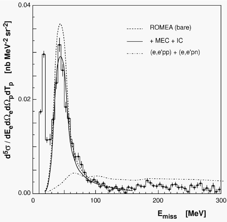
Figure 25: Data from this work together with calculations by the Ghent Group for the $E_{\rm miss}$-dependence of the cross-section data obtained in dip-region kinematics for $E_{\rm beam}$ $=$ 1.643 GeV. Uncertainties are statistical and, on average, there is an additional $\pm$5.9% systematic uncertainty (see Table 29) associated with the data.

Table 29: Measured cross-section data for proton knockout from ¹⁶O for $E_{\rm beam}$ $=$ 1.643 GeV in dip-region kinematics for $E_{\rm miss}$ $>$ 25 MeV. There is an additional 5.9% systematic uncertainty associated with these results.

$E_{\rm miss}$	$<p_{\rm miss}>$	$d^{6}\sigma/d\omega dE_{p}d\Omega_{e}d\Omega_{p}$
(MeV)	(MeV/$c$)	(nb/MeV2/sr2)
27.5	163.6	0.0115 $\pm$ 0.0012
32.5	152.1	0.0158 $\pm$ 0.0012
37.5	138.8	0.0235 $\pm$ 0.0013
42.5	132.8	0.0316 $\pm$ 0.0015
47.5	128.3	0.0262 $\pm$ 0.0013
52.5	119.4	0.0184 $\pm$ 0.0011
57.5	112.1	0.0160 $\pm$ 0.0011
62.5	107.5	0.0107 $\pm$ 0.0009
67.5	95.0	0.0078 $\pm$ 0.0009
72.5	95.0	0.0079 $\pm$ 0.0008
77.5	95.0	0.0062 $\pm$ 0.0007
82.5	90.0	0.0045 $\pm$ 0.0006
87.5	84.0	0.0028 $\pm$ 0.0005
92.5	76.0	0.0025 $\pm$ 0.0005
97.5	71.7	0.0030 $\pm$ 0.0005
102.5	68.0	0.0025 $\pm$ 0.0005
107.5	60.0	0.0015 $\pm$ 0.0004
112.5	61.4	0.0022 $\pm$ 0.0004
117.5	58.0	0.0013 $\pm$ 0.0004
122.5	51.0	0.0006 $\pm$ 0.0004
127.5	47.5	0.0010 $\pm$ 0.0004
132.5	50.0	0.0015 $\pm$ 0.0005
137.5	60.0	0.0007 $\pm$ 0.0005
142.5	45.0	0.0012 $\pm$ 0.0006
147.5	39.0	0.0002 $\pm$ 0.0004
152.5	39.3	0.0014 $\pm$ 0.0004
157.5	48.8	0.0012 $\pm$ 0.0004
162.5	51.7	0.0009 $\pm$ 0.0004
167.5	55.0	0.0019 $\pm$ 0.0004
172.5	62.0	0.0016 $\pm$ 0.0004
177.5	65.9	0.0015 $\pm$ 0.0004
177.5	65.9	0.0015 $\pm$ 0.0004
182.5	69.0	0.0028 $\pm$ 0.0005
187.5	77.2	0.0023 $\pm$ 0.0005
192.5	94.0	0.0017 $\pm$ 0.0004
197.5	97.7	0.0016 $\pm$ 0.0005
202.5	97.7	0.0020 $\pm$ 0.0005
207.5	103.0	0.0015 $\pm$ 0.0005
212.5	114.1	0.0014 $\pm$ 0.0005
217.5	118.3	0.0009 $\pm$ 0.0004
222.5	122.3	0.0019 $\pm$ 0.0005
227.5	125.9	0.0020 $\pm$ 0.0005
232.5	135.0	0.0013 $\pm$ 0.0005
237.5	150.5	0.0014 $\pm$ 0.0006
242.5	157.7	0.0011 $\pm$ 0.0005
247.5	157.7	0.0004 $\pm$ 0.0004
252.5	167.0	0.0018 $\pm$ 0.0005
257.5	170.0	0.0013 $\pm$ 0.0005
262.5	173.2	0.0018 $\pm$ 0.0006
267.5	179.5	0.0022 $\pm$ 0.0006
272.5	185.9	0.0008 $\pm$ 0.0005
277.5	188.0	0.0012 $\pm$ 0.0006
282.5	210.0	0.0006 $\pm$ 0.0005
287.5	200.0	0.0017 $\pm$ 0.0006
292.5	200.0	0.0004 $\pm$ 0.0006
297.5	205.0	0.0009 $\pm$ 0.0006

References

- Frullani and Mougey (1984) S. Frullani and J. Mougey, in Advances in Nuclear Physics, edited by J. W. Negel and E. Vogt (Plenum Press, New York, 1984), vol. 14, p. 1, eprint and references therein.
- Kelly (1996) J. J. Kelly, Adv. Nucl. Phys. 23, 75 (1996), eprint and references therein.
- Boffi et al. (1996) S. Boffi, C. Giusti, F. D. Pacati, and M. Radici, Electromagnetic Response of Atomic Nuclei (Oxford University Press, Oxford, 1996).
- Kelly (1997) J. J. Kelly, Phys. Rev. C. 56, 2672 (1997).
- Amaldi et al. (1967) U. Amaldi et al., Phys. Lett. B. 25, 24 (1967).
- Mougey et al. (1976) J. Mougey et al., Nucl. Phys. A262, 461 (1976).
- Picklesimer et al. (1985) A. Picklesimer, J. W. Van Orden, and S. J. Wallace, Phys. Rev. C. 32, 1312 (1985).
- Picklesimer and Van Orden (1987) A. Picklesimer and J. W. Van Orden, Phys. Rev. C. 35, 266 (1987).
- Picklesimer and Van Orden (1989) A. Picklesimer and J. W. Van Orden, Phys. Rev. C. 40, 290 (1989).
- Müther and Dickhoff (1994) H. Müther and W. H. Dickhoff, Phys. Rev. C. 49, R17 (1994).
- Bernheim et al. (1982) M. Bernheim et al., Nucl. Phys. A375, 381 (1982).
- Chinitz et al. (1991) L. Chinitz et al., Phys. Rev. Lett. 67, 568 (1991).
- Spaltro et al. (1993) C. M. Spaltro et al., Phys. Rev. C. 48, 2385 (1993).
- Leuschner et al. (1994) M. Leuschner et al., Phys. Rev. C. 49, 955 (1994).
- Blomqvist et al. (1995a) K. I. Blomqvist et al., Phys. Lett. B. 344, 85 (1995a).
- Udías et al. (1993) J. M. Udías, P. Sarriguren, E. Moya de Guerra, E. Garrido, and J. A. Caballero, Phys. Rev. C. 48, 2731 (1993).
- Hummel and Tjon (1994) E. Hummel and J. A. Tjon, Phys. Rev. C. 49, 21 (1994).
- Udías et al. (1995) J. M. Udías, P. Sarriguren, E. Moya de Guerra, E. Garrido, and J. A. Caballero, Phys. Rev. C. 51, 3246 (1995).
- Caballero et al. (1998a) J. A. Caballero, T. W. Donnelly, E. Moya de Guerra, and J. M. Udías, Nucl. Phys. A643, 189 (1998a).
- Udías et al. (1999) J. M. Udías, J. A. Caballero, E. Moya de Guerra, J. E. Amaro, and T. W. Donnelly, Phys. Rev. Lett. 83, 5451 (1999).
- Udías and Vignote (2000) J. M. Udías and J. R. Vignote, Phys. Rev. C. 62, 034302 (2000).
- Lourie et al. (1986) R. Lourie et al., Phys. Rev. Lett. 56, 2364 (1986).
- Ulmer et al. (1987) P. E. Ulmer et al., Phys. Rev. Lett. 59, 2259 (1987).
- Weinstein et al. (1990) L. B. Weinstein et al., Phys. Rev. Lett. 64, 1646 (1990).
- Holtrop et al. (1998) M. Holtrop et al., Phys. Rev. C. 58, 3205 (1998).
- Morrison et al. (1999) J. H. Morrison et al., Phys. Rev. C. 59, 221 (1999).
- Lanen et al. (1990) J. B. J. M. Lanen et al., Phys. Rev. Lett. 64, 2250 (1990).
- van der Steenhoven et al. (1988) G. van der Steenhoven et al., Nucl. Phys. A480, 547 (1988).
- Dutta et al. (2000) D. Dutta et al., Phys. Rev. C. 61, 061602(R) (2000).
- (30) D. Dutta, eprint Ph. D. thesis, Northwestern University (1999), see also nucl-ex/0305005.
- Takaki (1989) T. Takaki, Phys. Rev. C. 39, 359 (1989).
- Ryckebusch et al. (1997) J. Ryckebusch et al., Nucl. Phys. A624, 581 (1997).
- Gil et al. (1997) A. Gil, J. Nieves, and E. Oset, Nucl. Phys. A627, 599 (1997).
- Saha et al. (1989) A. Saha, W. Bertozzi, R. W. Lourie, and L. B. Weinstein, Experiment Proposal E89-003, Jefferson Laboratory (1989), eprint see also http://www.jlab.org/exp_prog/experiments/summaries/.
- Fissum et al. (1997) K. G. Fissum et al., MIT-LNS Internal Report 2/97, Massachusetts Institute of Technology (1997), eprint see also http://hallaweb.jlab.org/experiment/E89-003/e89003.html.
- (36) eprint http://hallaweb.jlab.org/.
- (37) eprint http://www.jlab.org/.
- (38) J. Alcorn et al., eprint accepted for publication in Nucl. Instrum. Methods Phys. Res. Sect. A.
- Gao et al. (1998) J. Gao et al., MIT-LNS Internal Report 4/98, Massachusetts Institute of Technology (1998), eprint see also http://hallaweb.jlab.org/experiment/E89-003/e89003/learned/e89003-beamdel.ps.gz.
- bcm (2001) Hall A Operations Manual (2001), eprint see also http://hallaweb.jlab.org/document/OPMAN/index.html.
- Unser (1981) K. B. Unser, IEEE Trans. Nuc. Sci. 28, 2344 (1981).
- Ulmer (1998) P. E. Ulmer, Internal Report to the E89-003 Collaboration, Old Dominion University (1998), eprint see also http://hallaweb.jlab.org/experiment/E89-003/e89003/learned/e89003-charge.ps.gz.
- Barry et al. (1990) W. Barry et al., Technical Memorandum JLAB-TN-90-246, Jefferson Laboratory (1990).
- Barry et al. (1991) W. Barry et al., Technical Memorandum JLAB-TN-91-087, Jefferson Laboratory (1991).
- (45) eprint http://www.aps.anl.gov/epics.
- Sinclair (1992) C. K. Sinclair, Technical Memorandum JLAB-TN-92-064, Jefferson Laboratory (1992).
- Garibaldi et al. (1992) F. Garibaldi et al., Nucl. Instrum. Methods Phys. Res. Sect. A 314, 1 (1992).
- (48) eprint http://hallaweb.jlab.org/equipment/high_resol.html.
- Liyanage et al. (1998) N. Liyanage et al., MIT-LNS Internal Report 5/98, Massachusetts Institute of Technology (1998), eprint see also http://hallaweb.jlab.org/experiment/E89-003/e89003/learned/e89003-optics.ps.gz.
- Liang (1998) M. Liang, Technical Memorandum JLAB-TN-99-029, Jefferson Laboratory (1998), eprint see also http://hallaweb.jlab.org/experiment/E89-003/e89003/learned/survey_summary.ps.gz.
-
(51)
eprint http://hallaweb.jlab.org/equipment/detectors/detectors.html;
http://hallaweb.jlab.org/equipment/detectors/trig.html. - Fissum et al. (2001) K. G. Fissum et al., Nucl. Instrum. Methods Phys. Res. Sect. A 474, 108 (2001).
- Fissum et al. (2000) K. G. Fissum et al., Technical Memorandum JLAB-TN-00-016, Jefferson Laboratory (2000), eprint see also http://hallaweb.jlab.org/equipment/vdc/vdcs.html.
- Iodice et al. (1998) M. Iodice et al., Nucl. Instrum. Methods Phys. Res. Sect. A 411, 223 (1998), eprint see also http://hallaweb.jlab.org/equipment/detectors/gas.html.
- (55) eprint http://hallaweb.jlab.org/equipment/acquisition.html.
- (56) eprint http://coda.jlab.org/.
- (57) eprint http://hallaweb.jlab.org/equipment/daq/dplot.html.
- (58) eprint http://pierre.mit.edu/compserv/abacus/.
- (59) eprint http://hallaweb.jlab.org/espace/index.html.
- Gao (1999) J. Gao, Ph.D. thesis, Massachusetts Institute of Technology (1999).
- Liyanage (1999) N. Liyanage, Ph.D. thesis, Massachusetts Institute of Technology (1999).
- Owens (1990) R. Owens, Nucl. Instrum. Methods Phys. Res. Sect. A 288, 574 (1990).
- Baghaei (1988) H. Baghaei, Ph.D. thesis, Massachusetts Institute of Technology (1988).
- Simon et al. (1980) G. G. Simon, C. Schmitt, F. Borkowski, and V. H. Walther, Nucl. Phys. A333, 381 (1980).
- Price et al. (1971) L. E. Price et al., Phys. Rev. D. 4, 45 (1971).
- (66) eprint http://www.jlab.org/~mliang/deadtime_cor/.
- Quint (1998) E. Quint, Ph.D. thesis, University of Amsterdam (1998).
- Florizone (1999) R. Florizone, Ph.D. thesis, Massachusetts Institute of Technology (1999).
- Borie and Drechsel (1971) E. Borie and D. Drechsel, Nucl. Phys. A167, 369 (1971).
- Templon et al. (2000) J. Templon, C. E. Vallidis, R. E. J. Florizone, and A. J. Sarty, Phys. Rev. C. 61, 014607 (2000).
- (71) eprint http://www.physics.odu.edu/~ulmer/mceep/mceep.html.
- Raskin and Donnelly (1989) A. S. Raskin and T. W. Donnelly, Ann. Phys. 191, 78 (1989).
- Rosenbluth (1950) M. N. Rosenbluth, Phys. Rev. 79, 615 (1950).
- Fissum and Ulmer (2002) K. G. Fissum and P. E. Ulmer, Technical Memorandum JLAB-TN-02-015, Jefferson Laboratory (2002), eprint see also http://hallaweb.jlab.org/experiment/E89-003/e89003/learned/e89003_sysun_us.ps.gz.
- Traini et al. (1988) M. Traini, S. Turck-Chièze, and A. Zghiche, Phys. Rev. C. 38, 2799 (1988).
- (76) J. M. Udías, eprint Ph. D. thesis, Universidad Autonoma de Madrid (1993).
- McDermott (1990) J. P. McDermott, Phys. Rev. Lett. 65, 1991 (1990).
- Jin et al. (1992) Y. Jin, D. S. Onley, and L. E. Wright, Phys. Rev. C 45, 1311 (1992).
- Hedayati-Poor et al. (1995) M. Hedayati-Poor, J. I. Johansson, and H. S. Sherif, Phys. Rev. C. 51, 2044 (1995).
- Kelly (1999a) J. J. Kelly, Phys. Rev. C. 60, 044609 (1999a).
- Meucci et al. (2001) A. Meucci, C. Giusti, and F. D. Pacati, Phys. Rev. C. 64, 014604 (2001).
- Caballero et al. (1998b) J. A. Caballero, T. W. Donnelly, E. Moya de Guerra, and J. M. Udías, Nucl. Phys. A632, 323 (1998b).
- de Forest Jr. (1983) T. de Forest Jr., Nucl. Phys. A392, 232 (1983).
- Chinn and Picklesimer (1992) C. R. Chinn and A. Picklesimer, Il Nuovo Cimento 105A, 1149 (1992).
- Rose (1961) M. E. Rose, Relativistic Electron Scattering (Wiley, New York, 1961).
- Satchler (1983) G. R. Satchler, Direct Nuclear Reactions (Oxford University Press, Oxford, 1983).
- Rawitscher (1997) G. Rawitscher, Phys. Rev. C. 56, 2029 (1997).
- Kelly (1999b) J. J. Kelly, Phys. Rev. C. 59, 3256 (1999b).
- (89) J. J. Kelly, eprint http://www.physics.umd.edu/enp/jjkelly/LEA.
- Radici et al. (2002) M. Radici, W. H. Dickhoff, and E. Roth Stoddard, Phys. Rev. C. 66, 014613 (2002).
- Radici et al. (2003) M. Radici, A. Meucci, and W. H. Dickhoff, Eur. Phys. J. A17, 65 (2003).
- Boffi et al. (1987) S. Boffi, C. Giusti, and F. D. Pacati, Il Nuovo Cimento 98A, 291 (1987).
- Jin and Onley (1994) Y. Jin and D. S. Onley, Phys. Rev. C. 50, 377 (1994).
- Martínez et al. (2002) M. C. Martínez, J. A. Caballero, and T. W. Donnelly, Nucl. Phys. A707, 83 (2002).
- Schiff (1956) L. L. Schiff, Phys. Rev. 103, 443 (1956).
- Giusti and Pacati (1987) C. Giusti and F. D. Pacati, Nucl. Phys. A473, 717 (1987).
- Kelly (2003) J. J. Kelly, Internal Report to the E89-003 Collaboration, University of Maryland (2003), eprint see also http://hallaweb.jlab.org/experiment/E89-003/e89003/publications/comparison.ps.gz.
- Sharma et al. (1993) M. M. Sharma, M. A. Nagarajan, and P. Ring, Phys. Lett. B. 312, 377 (1993).
- Cooper et al. (1993) E. D. Cooper, S. Hama, B. C. Clark, and R. L. Mercer, Phys. Rev. C. 47, 297 (1993).
- Debruyne et al. (2000) D. Debruyne, J. Ryckebusch, W. V. Nespen, and S. Janssen, Phys. Rev. C. 62, 024611 (2000).
- Debruyne and Ryckebusch (2002) D. Debruyne and J. Ryckebusch, Nucl. Phys. A699, 65 (2002).
- Debruyne et al. (2002) D. Debruyne, J. Ryckebusch, S. Janssen, and T. V. Cauteren, Phys. Lett. B527, 67 (2002).
- Ryckebusch et al. (2003) J. Ryckebusch, D. Debruyne, P. Lava, S. Janssen, B. V. Overmeire, and T. V. Cauteren, Nucl. Phys. A728, 226 (2003), eprint see also nucl-th/0305066.
- Hagiwara et al. (2002) K. Hagiwara et al., Phys. Rev. D. 66, 01001 (2002).
- Ryckebusch and Debruyne (2002) J. Ryckebusch and D. Debruyne, Internal Report to the E89-003 Collaboration, Ghent University (2002), eprint see also http://hallaweb.jlab.org/experiment/E89-003/e89003/publications/gentcal.ps.gz.
- Furnstahl et al. (1997) R. J. Furnstahl, B. D. Serot, and H.-B. Tang, Nucl. Phys. A615, 441 (1997).
- Gao et al. (2000) J. Gao et al., Phys. Rev. Lett. 84, 3265 (2000).
- Liyanage et al. (2001) N. Liyanage et al., Phys. Rev. Lett. 86, 5670 (2001).
- Udías and Vignote (2001) J. M. Udías and J. R. Vignote, Internal Report to the E89-003 Collaboration, Universidad Complutense de Madrid (2001), eprint see also http://hallaweb.jlab.org/experiment/E89-003/e89003/publications/udvig89003f.ps.gz.
- Horowitz and Serot (1981) C. Horowitz and B. Serot, Nucl. Phys. A368, 503 (1981).
- Horowitz et al. (1991) C. J. Horowitz, D. P. Murdock, and B. D. Serot, Computational Nuclear Physics (Springer, Berlin, 1991).
- Udías et al. (2001) J. M. Udías et al., Phys. Rev. C. 64, 024614 (2001), eprint see also nucl-th/0101038.
- McNeil et al. (1983) J. A. McNeil, L. Ray, and S. J. Wallace, Phys. Rev. C. 27, 2123 (1983).
- Horowitz (1985) C. J. Horowitz, Phys. Rev. C. 31, 1340 (1985).
- Murdock (1987) D. P. Murdock, Phys. Rev. C. 35, 1442 (1987).
- Gari and Krümpelmann (1985) M. Gari and W. Krümpelmann, Z. Phys. A322, 689 (1985).
- Lu et al. (1998) D. H. Lu, A. W. Thomas, K. Tsushima, A. G. Williams, and K. Saito, Phys. Lett. B. 417, 217 (1998).
- Lu et al. (1999) D. H. Lu, K. Tsushima, A. W. Thomas, A. G. Williams, and K. Saito, Phys. Rev. C. 60, 068201 (1999).
- Saha et al. (2000) A. Saha, W. Bertozzi, L. B. Weinstein, and K. G. Fissum, Experiment Proposal E00-102, Jefferson Laboratory (2000), eprint see also http://www.jlab.org/exp_prog/experiments/summaries/ and http://hallaweb.jlab.org/experiment/E00-102/e00102/e00102.html.
- Amaro et al. (1999) J. E. Amaro, A. M. Lallena, and J. A. Caballero, Phys. Rev. C. 60, 014602 (1999).
- Amaro et al. (2003) J. E. Amaro, M. B. Barbaro, J. A. Caballero, and F. K. Tabatabaei, Phys. Rev. C. 68, 014604 (2003).
- Ryckebusch et al. (1999) J. Ryckebusch, D. Debruyne, W. Van Nespen, and S. Janssen, Phys. Rev. C. 60, 034604 (1999).
- Ryckebusch (2001) J. Ryckebusch, Phys. Rev. C. 64, 044607 (2001).
- Ryckebusch et al. (1992) J. Ryckebusch, K. Heyde, L. Machenil, D. Ryckbosch, M. Vanderhaeghen, and M. Waroquier, Phys. Rev. C. 46, R829 (1992).
- Janssen et al. (2000) S. Janssen et al., Nucl. Phys. A672, 285 (2000).
- Kelly (2002) J. J. Kelly, Internal Report to the E89-003 Collaboration, University of Maryland (2002), eprint see also http://hallaweb.jlab.org/experiment/E89-003/e89003/publications/survey.ps.gz.
- Mergell et al. (1996) P. Mergell, U. G. Meiner, and D. Dreschsel, Nucl. Phys. A596, 367 (1996).
- Barbieri and Dickhoff (2002) C. Barbieri and W. H. Dickhoff, Phys. Rev. C. 65, 064313 (2002).
- Lapikás et al. (2000) L. Lapikás, G. van der Steenhoven, L. Frankfurt, M. Strikman, and M. Zhalov, Phys. Rev. C. 61, 064325 (2000).
- Blomqvist et al. (1995b) K. I. Blomqvist et al., Z. Phys. A351, 353 (1995b).
- Frankfurt et al. (2001) L. Frankfurt, M. Strikman, and M. Zhalov, Phys. Lett. B. 503, 73 (2001).
- Day et al. (1990) D. B. Day et al., Ann. Rev. Nucl. Part. Sci. 40, 357 (1990).