Elliptic flow contribution to two-particle correlations at different orientations to the reaction plane

Abstract

Collective anisotropic particle flow, a general phenomenon present in relativistic heavy-ion collisions, can be separated from direct particle-particle correlations of different physics origin by virtue of its specific azimuthal pattern. We provide expressions for flow-induced two-particle azimuthal correlations, if one of the particles is detected under fixed directions with respect to the reaction plane. We consider an ideal case when the reaction plane angle is exactly known, as well as present the general expressions in case of finite event-plane resolution. We foresee applications for the study of generic two-particle correlations at large transverse momentum originating from jet fragmentation.

I Introduction

Collective particle flow is a general phenomenon of relativistic heavy-ion collisions that originates from pressure gradients built up in the anisotropic overlap zone of colliding nuclei ollitrault92 . Azimuthal anisotropies in inclusive single particle distributions relative to the reaction plane (anisotropic flow) have been extensively studied e877 ; na49 ; ceres ; star ; phenix ; phobos . Recent investigations of direct two (or more) particle correlations also indicate that the dependence of these correlations on the orientation of the reaction plane may contain important physics information. A detailed analysis of such correlations requires flow effects to be taken into account.

A recent example, which gave the motivation for this paper, is provided by azimuthal two-particle correlations at transverse momenta above 1 GeV/c. Such particles presumably originate from fragmentation of dijets, but are embedded in collective flow ceres . It is predicted that nuclear effects may modify the jet fragmentation function due to induced radiation of the leading parton quenching . This could result in significant changes in the particle correlations within the jet, as well as the correlation of particles originating from back-to-back jets. The modifications of the jet profile may depend on the nuclear geometry and could be studied relative to the reaction plane angle ceres .

In this paper, we present analytical formulae for the flow contribution to two-particle azimuthal distributions for different orientations of the trigger particle with respect to the reaction plane, neglecting any non-flow effects. We will first discuss an ideal case with the reaction plane angle exactly known and then incorporate the finite resolution of the reconstructed event plane.

II Anisotropic transverse flow

Anisotropic flow manifests itself by the presence of higher ($n\geq 1$) harmonics in the inclusive single particle distribution in the azimuthal angle $\phi$ with respect to the reaction plane $\Psi_{R}$ e877 ; vol :

$$\frac{dN}{d(\phi-\Psi_{R})}\propto(1+\sum_{n=1}^{\infty}2\;v_{n}\cos(n(\phi-\Psi_{R}))).$$ (1)

The Fourier coefficients, $v_{n}=\langle\cos(n(\phi-\Psi_{R}))\rangle$, given by the average over detected particles in analyzed events quantify the anisotropy of the $n-$th harmonic of the distribution. The anisotropies corresponding to the first and the second Fourier coefficients, $v_{1}$ and $v_{2}$, are usually referred to as directed and elliptic flow, respectively.

Collective flow generates azimuthal anisotropies also in the angle difference $\Delta\phi=\phi_{i}-\phi_{j}$ ($0\leq\Delta\phi\leq\pi$) of particle pairs pair ,

$$\!\frac{dN^{pairs}}{\pi\,d\Delta\phi}\!=B\,(1\!+\!\sum_{n=1}^{\infty}2\;p_{n}(p_{Ti},y_{i};p_{Tj},y_{j})\cos(n\Delta\phi)),$$ (2)

where $B$ denotes the integrated inclusive pair yield. In case of pure collective flow, the Fourier coefficients $p_{n}=\langle\cos(n\Delta\phi)\rangle$ are given by posk

$$p_{n}(p_{Ti},y_{i};p_{Tj},y_{j})=v_{n}(p_{Ti},y_{i})\,v_{n}(p_{Tj},y_{j}).$$ (3)

III Pair distributions in $\Delta\phi$ when the trigger particle is detected at fixed angle relative to the event plane

We introduce conditional two-particle correlations in the transverse plane for which one of the particles, usually referred to as the trigger particle, is detected within some bi-sector ${\cal R}$ at fixed orientation with respect to the reaction plane, see Fig. 1.

The $n$-th harmonic of the pair distribution, before given by Eq. (3), is expressed as

$$p_{n}^{\cal R}=v_{n}(p_{T},y)\;v_{n}^{\cal R}(p_{T},y).$$ (4)

To simplify the notations, we have assumed that both particles are detected in the same $p_{T}$ and $y$ interval, but it is straightforward to generalize our results for the case when the trigger particle and the associated particle are chosen from different rapidity and transverse momentum regions. Here, $v_{n}^{\cal R}=\langle\cos(n(\phi-\Psi))\rangle^{\cal R}$ is the $n$-th harmonic coefficient of the single-particle distribution of Eq. (1), although the average over the azimuthal angle of the trigger particle is taken over the restricted region ${\cal R}$ only.

We derive now explicit analytic expressions for $v_{2}^{\cal R}$ and the pair yield $B^{\cal R}$ for elliptic flow when the trigger particle is confined to a bi-sector oriented with angle $\phi_{S}$ to the reaction plane, and then specialize to in-plane and out-of-plane conditions. We proceed in two steps, first for the ideal case, then for finite resolution in the reconstructed event plane.

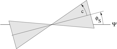
Figure 1: The region ${\cal R}$ is made up of a bi-sector of half-angle $c$ that intersects the reaction plane $\Psi$ at angle $\phi_{S}$, modulo $\pi$.

III.1 Ideal case. Reaction plane is known.

Let the trigger particle be confined in the transverse plane to the bi-sectors depicted in Fig. 1. The $n$-th Fourier coefficient of the trigger particle distribution, assuming it is originally given by Eq. (1), is

$$v_{n}^{\cal{R}} = \langle\cos(n(\phi-\Psi_{R}))\rangle^{\cal{R}}=\frac{\int\limits_{\cal{R}}(1+\sum\limits_{k=1}^{\infty}2v_{k}\cos(k(\phi-\Psi_{R})))\cos(n(\phi-\Psi_{R}))d(\phi-\Psi_{R})}{\int\limits_{\cal{R}}(1+\sum\limits_{k=1}^{\infty}2v_{k}\cos({k}(\phi-\Psi_{R})))d(\phi-\Psi_{R})},$$ (5)

where the integration over the region ${\cal R}$ in more explicit notation is understood to read

$$\int\limits_{\cal{R}}d(\phi-\Psi_{R})\;.\;.\;.\equiv\int\limits_{\phi_{S}-c}^{\phi_{S}+c}d(\phi-\Psi_{R})\;.\;.\;.+\int\limits_{\phi_{S}+\pi-c}^{\phi_{S}+\pi+c}d(\phi-\Psi_{R})\;.\;.\;.\;\;.$$ (6)

The integration results in

$$v_{n}^{\cal R}=\frac{v_{n}+\delta_{n,even}\cos(n\phi_{S})\frac{{\textstyle\sin(nc)}}{\textstyle{nc}}+\sum\limits_{k=2,4,6,...}({\textstyle v_{k+n}+v_{|k-n|}})\cos(k\phi_{S})\frac{\textstyle{\sin(kc)}}{\textstyle{kc}}}{1+\sum\limits_{k=2,4,6,...}{\textstyle 2\,v_{k}}\cos(k\phi_{S})\frac{\textstyle{\sin(kc)}}{\textstyle{kc}}},$$ (7)

where $\delta_{n,even}$ = 1 for $n$ even and $\delta_{n,even}$ = 0 for $n$ odd, respectively.

Spatial conditions on the trigger particle also modify the integrated pair yield. We express the conditional two-particle yield as

$$B^{\cal R}=\frac{2c}{\pi}\,B\,\beta^{\cal R},$$ (8)

which can be understood as the product of two single-particle yields: $\sqrt{B}$ for the associated particle and the remainder $\sqrt{B}\,\frac{\textstyle{2c}}{\textstyle{\pi}}\,\beta^{\cal R}$ for the trigger particle. Here, $\frac{\textstyle{2c}}{\textstyle{\pi}}$ is the fraction of the azimuth covered by the trigger particle and the quantity $\beta^{\cal R}$ accounts for the modification of the yield due to collective flow and is given by

$$\beta^{\cal R}=\frac{{\int\limits_{\cal{R}}(1+\sum\limits_{k=2,4,6,...}2v_{k}\cos(k(\phi-\Psi_{R})))d(\phi-\Psi_{R})}}{\int\limits_{\cal{R}}\,d(\phi-\Psi_{R})}.$$ (9)

Integrating we obtain

$$\beta^{\cal R}=1+\sum\limits_{k=2,4,6,...}2\,v_{k}\cos(k\phi_{S})\frac{\textstyle\sin(kc)}{kc}.$$ (10)

In the following we restrict ourselves to elliptic flow ($n$ = 2). Neglecting terms with $n\geq$ 4, we obtain

$$v_{2}^{\cal{R}}=\frac{v_{2}+\displaystyle\cos(2\phi_{S})\frac{\textstyle{\sin(2c)}}{\textstyle{2c}}+v_{2}\cos(4\phi_{S})\frac{\textstyle{\sin(4c)}}{\textstyle{4c}}}{1+\displaystyle 2v_{2}\cos(2\phi_{S})\frac{\textstyle{\sin(2c)}}{\textstyle{2c}}},$$ (11)

and

$$\beta^{\cal{R}}=1+2v_{2}\cos(2\phi_{S})\,\frac{\textstyle{\sin(2c)}}{\textstyle{2c}}.$$ (12)

If the trigger particle is confined to regions $-\pi/4<\phi-\Psi_{R}<\pi/4$ ($\phi_{S}$ = 0, ’in-plane’ ), and $\pi/4<\phi-\Psi_{R}<3\pi/4$ ($\phi_{S}=\pi/2$, ’out-of-plane’ ), respectively, Eq. (11) simplifies to

$$v_{2}^{\rm in}=\frac{\pi v_{2}+2}{\pi+4v_{2}},~{}~{}~{}v_{2}^{\rm out}=\frac{\pi v_{2}-2}{\pi-4v_{2}}.$$ (13)

Figure 2: In-plane and out-of-plane correlation functions for ideal reaction plane (full lines), and for finite event plane resolution ($\langle\cos(2\Delta\Psi)\rangle=0.3$) (dashed lines). The trigger particle is confined to bi-sectors with axes $\phi_{S}$ pointing along the reaction plane ($\phi_{S}=\Psi$) and perpendicular to it ($\phi_{S}=\Psi+\pi/2$), respectively. The magnitude of elliptic flow is $v_{2}$ = 10%.

The pair yields under these conditions are

$$B^{\rm in}=\frac{B}{2}\left(1+\frac{4v_{2}}{\pi}\right),~{}~{}~{}B^{\rm out}=\frac{B}{2}\left(1-\frac{4v_{2}}{\pi}\right)$$ (14)

which add up to $B$ as both regions cover together the full azimuth.

The azimuthal distributions for in and out-of-plane conditions are obtained by inserting the corresponding expressions for $v_{2}^{\cal{R}}$ into Eq. (4) and then $p_{2}^{\cal{R}}$ and $B^{\cal{R}}$ into Eq. (2). The normalized in-plane and out-of-plane distributions for $v_{2}$ = 0.1 are displayed in Fig. 2 (full line). The out-of-plane distribution is shifted in phase by $\pi/2$ compared to the in-plane distribution: instead of peaks at $\Delta\phi=$ 0 and $\pi$ peaks show up at $\pi/2$ and $3\pi/2$. The sign of $v_{2}^{\rm out}$ is negative. Both curves touch at level $(B/2)(1-2v_{2}^{2})$.

III.2 Finite event plane resolution

The direction of the true reaction plane $\Psi_{R}$ is not available experimentally. An estimator for the reaction plane, often called the event plane, $\Psi_{E}$, is determined event-by-event using the anisotropic flow itself posk . How close on average the event plane is to the true reaction plane is determined by the resolution, usually quantified by $\langle\cos(n\Delta\Psi)\rangle$, where $\Delta\Psi=\Psi_{E}-\Psi_{R}$. Here, the angular brackets $\langle\cdots\rangle$ indicate the event averaging over the probability density distribution $\rho(\Delta\Psi)$ that characterizes the event plane resolution.

Figure 3: In-plane (thick lines) and out-of-plane coefficients (thin lines) $p_{2}$ of Eq. (4), (top), and $B$ of Eq. (8), (bottom), vs elliptic flow anisotropy $v_{2}$. Solid lines assume ideal reaction plane, dashed lines are for reconstructed event planes with finite resolution $\langle\cos(2\Delta\Psi)\rangle=0.3$.

Let us now calculate how the finite event plane resolution modifies our results. For a given deviation $\Delta\Psi$ the new range of integration $\widetilde{\cal{R}}$ in Eq. (5) and Eq. (9) is defined in analogy to Eq. (6) by

$$\int\limits_{\widetilde{\cal{R}}}d(\phi-\Psi_{R})\;.\;.\;.\equiv\int\limits_{\phi_{S}+\Delta\Psi-c}^{\phi_{S}+\Delta\Psi+c}d(\phi-\Psi_{R})\;.\;.\;.+\int\limits_{\phi_{S}+\Delta\Psi+\pi-c}^{\phi_{S}+\Delta\Psi+\pi+c}d(\phi-\Psi_{R})\;.\;.\;.\;\;.$$ (15)

The $n$-th Fourier harmonic component is obtained after averaging over the probability density distribution $\rho(\Delta\Psi)$,

$$\widetilde{v_{n}^{\cal{R}}}=\frac{\int\limits_{-\pi}^{\pi}\rho(\Delta\Psi)\;\int\limits_{\widetilde{\cal{R}}}(1+\sum\limits_{k=1}^{\infty}2v_{k}\cos(k(\phi-\Psi_{R})))\cos(n(\phi-\Psi_{R}))d(\phi-\Psi_{R})\;d(\Delta\Psi)}{\int\limits_{-\pi}^{\pi}\rho(\Delta\Psi)\;\int\limits_{\widetilde{\cal{R}}}(1+\sum\limits_{k=1}^{\infty}2v_{k}\cos(k(\phi-\Psi_{R})))d(\phi-\Psi_{R})\;d(\Delta\Psi)}.$$ (16)

After integration we obtain

$$\widetilde{v_{n}^{\cal R}}=\frac{v_{n}+\delta_{n,even}\cos(n\phi_{S})\frac{{\textstyle\sin(nc)}}{\textstyle{nc}}\langle\cos(n\Delta\Psi)\rangle+\sum\limits_{k=2,4,6,...}({\textstyle v_{k+n}+v_{|k-n|}})\cos(k\phi_{S})\frac{\textstyle{\sin(kc)}}{\textstyle{kc}}\langle\cos(k\Delta\Psi)\rangle}{1+\sum\limits_{k=2,4,6,...}{\textstyle 2\,v_{k}}\cos(k\phi_{S})\frac{\textstyle{\sin(kc)}}{\textstyle{kc}}\langle\cos(k\Delta\Psi)\rangle}.$$ (17)

In analogy, we can write

$$\widetilde{\beta^{\cal R}}=\frac{\int\limits_{-\pi}^{\pi}\rho(\Delta\Psi)\int\limits_{\widetilde{\cal{R}}}(1+\sum\limits_{k=2,4,6,...}2v_{k}\cos(k(\phi-\Psi_{R})))d(\phi-\Psi_{R})d(\Delta\Psi)}{\int\limits_{\widetilde{\cal{R}}}\,d(\phi-\Psi_{R})}.$$ (18)

After integration we obtain:

$$\widetilde{\beta^{\cal R}}=1+\sum\limits_{k=2,4,6,...}\textstyle 2\,v_{k}\cos(k\phi_{S})\frac{\textstyle{\sin(kc)}}{\textstyle{kc}}\langle\cos(k\Delta\Psi)\rangle.$$ (19)

In the following we restrict ourselves again to elliptic flow ($n=$ 2) only, and neglecting terms with $n~{}\geq$ 4, we obtain

$$\widetilde{v_{2}^{\cal{R}}} = \frac{v_{2}+\displaystyle\cos(2\phi_{S})\frac{\textstyle{\sin(2c)}}{\textstyle{2c}}\langle\cos(2\Delta\Psi)\rangle+v_{2}\cos(4\phi_{S})\frac{\textstyle{\sin(4c)}}{\textstyle{4c}}\langle\cos(4\Delta\Psi)\rangle}{1+\displaystyle 2v_{2}\cos(2\phi_{S})\frac{\textstyle{\sin(2c)}}{\textstyle{2c}}\langle\cos(2\Delta\Psi)\rangle},$$ (20)

and

$$\widetilde{\beta^{\cal{R}}}=1+2v_{2}\cos(2\phi_{S})\,\frac{\textstyle{\sin(2c)}}{\textstyle{2c}}\langle\cos(2\Delta\Psi)\rangle.$$ (21)

The in-plane and out-of-plane anisotropies of Eq. (13) for elliptic flow are modified for finite event plane resolution to

$$\widetilde{v}_{2}^{\rm in} = \frac{\pi v_{2}+2\langle\cos(2\Delta\Psi)\rangle}{\pi+4v_{2}\langle\cos(2\Delta\Psi)\rangle},$$

$$\widetilde{v}_{2}^{\rm out} = \frac{\pi v_{2}-2\langle\cos(2\Delta\Psi)\rangle}{\pi-4v_{2}\langle\cos(2\Delta\Psi)\rangle},$$ (22)

and the average yields of Eq. (14) to

$$\widetilde{B}^{\rm in} = \frac{B}{2}\left[1+\frac{4v_{2}}{\pi}\langle\cos(2\Delta\Psi)\rangle\right],$$

$$\widetilde{B}^{\rm out} = \frac{B}{2}\left[1-\frac{4v_{2}}{\pi}\langle\cos(2\Delta\Psi)\rangle\right],$$ (23)

respectively. These formulae have been used to calculate the dashed lines in Fig. 2, and it is seen that the magnitude of the elliptic anisotropy is reduced for finite event plane resolution. The normalized background parameters $\widetilde{B}^{\rm in}/B$ and $\widetilde{B}^{\rm out}/B$ approach the value of 0.5. Both are consequences of the finite event plane resolution which causes the in-plane region to receive also negative contributions from the out-of-plane region, and vice versa.

Fig. 3 presents a synopsis of the dependence of the flow parameters under in-plane and out-of-plane conditions on the magnitude $v_{2}$ of elliptic flow, both for ideal as well as for the reconstructed event plane. For the latter case, the reaction plane resolution was chosen to be $\langle\cos(2\Delta\Psi)\rangle=0.3$. Note that very large $v_{2}$ and small $\langle\cos(2\Delta\Psi)\rangle$ could lead to the situation of $v_{2}^{\text{out}}>0$, and the phases of in-plane and out-of-plane distributions, Fig. 2, would be the same.

IV SUMMARY AND OUTLOOK

We have presented general expressions of two particle azimuthal correlations due to anisotropic flow for the case when one of the particles, referred to as the trigger particle, is detected at fixed angles relative to the reaction plane. Analytical formulae are given for two cases, an ideal case when the reaction plane is exactly known in every event, and for the case of finite reaction plane resolution. For the so called in-plane and out-of-plane conditions, we find that the correlation functions are shifted in phase by $\pi/2$ for realistic values of elliptic flow of the trigger particle and the reaction plane resolution. This and the increase in modulation amplitude in-plane compared to out-of-plane is easily visualized by the fact that the trigger particle scans the peak region of the elliptic flow pattern in the first case, but the valley in the second.

We foresee that the results presented in this paper will allow to disentangle non-flow generic two-particle correlations, like those due to jets and analyze how such correlations depend on the orientation of the jet with respect to the reaction plane.

References

[1]
J.-Y. Ollitrault, Phys. Rev. D 46, 229 (1992); Phys. Rev. D 48 1132 (1993).
[2]
E877 Collaboration, J. Barrette et al., Phys. Rev. Lett. 70, 2996 (1993);
Phys. Rev. C 55, 1420 (1997); Phys. Rev. C 56, 3254 (1997).
[3]
NA49 Collaboration, H. Appelshauser et al., Phys. Rev. Lett. 80, 4136 (1998);
C. Alt et al., Phys. Rev. C 68, 034903 (2003).
[4] CERES/NA45 Collaboration, G. Agakichiev et al., Phys.Rev.Lett. in print,
nucl-ex/0303014.
[5]
STAR Collaboration, C. Adler et al., Phys. Rev. Lett. 90, 032301 (2003);
K. H. Ackermann et al., Phys. Rev. Lett. 86, 402 (2001);
C. Adler et al., Phys. Rev. Lett. 87, 182301 (2001).
[6]
PHENIX Collaboration, K. Adcox et al., Phys. Rev. Lett. 89, 212301 (2002);
S.S. Adler et al., Phys. Rev. Lett. 91, 182301 (2003)
[7]
PHOBOS Collaboration, B.B. Back et al., Phys. Rev. Lett. 89, 222301 (2002);
[8]
M. Gyulassy and M. Plumer, Phys. Lett. B 243, 432 (1990);
X. N. Wang and M. Gyulassy, Phys. Rev. Lett. 68, 1480 (1992).
[9]
S. Voloshin and Y. Zhang, Z. Phys. C 70, 665 (1996).
[10]
S. Wang, Y.Z. Jiang, Y.M. Liu, D. Keane, D. Beavis, S.Y. Chu,
S.Y. Fung, M. Vient, C. Hartnack, and H. Stöcker, Phys. Rev. C 44, 1091 (1991).
[11]
A. M. Poskanzer and S. A. Voloshin, Phys. Rev. C 58, 1671 (1998).