Coordinatore:	Ch.mo Prof. Attilio Stella
Supervisore:	Ch.mo Prof. Maurizio Morando

Dottorando: Andrea Dainese

31 Ottobre 2003

Charm production and in-medium QCD energy loss in nucleus–nucleus collisions with ALICE.
A performance study.

Introduction

The search for quark–gluon plasma —the state of deconfined strongly interacting matter which is thought to have constituted the 1-$\mu$s-old Universe— received a big boost in the 1990s with the acceleration of heavy ions in the Super Proton Synchrotron at CERN. There, several fixed-target experiments gave results, on different physical observables, indicating that a new state of matter with unusual properties is formed in the early stage of the collisions. Heavy ion physics has now entered the collider era. Results from experiments at the Relativistic Heavy Ion Collider (RHIC) have provided further evidence for the long-sought quark–gluon plasma and encourage the study of its properties at the Large Hadron Collider (LHC), where energy densities of $\sim 100$-$600$ times the density of atomic nuclei will be reached in the collisions of lead nuclei at 5.5 TeV per nucleon–nucleon pair.

The recent results from RHIC suggest that it is possible to probe the dense medium formed in nucleus–nucleus collisions through the reduction in the production of high-momentum particles. This effect may be, indeed, due to an energy loss, or quenching, of the partons as they propagate through the medium. If this is the case, the new deconfined phase can be probed and investigated by means of a ‘tomography’ with beams of energetic partons.

At the LHC the probes being used at RHIC, light quarks and gluons, will extend their energy range by one order of magnitude and a new type of probe will become available with fairly high cross sections: heavy quarks.

The large masses of the charm and beauty quarks make them qualitatively different probes, since, on well-established quantum chromodynamics grounds, in-medium energy loss off massive partons is expected to be significantly smaller than off massless partons. Therefore, a comparative study of the attenuation of massless (gluons and light quarks) and massive probes is a promising tool to test the coherence of the interpretation of quenching effects as energy loss in a deconfined medium and to further investigate the properties of such medium.

In this work we focus on charm physics with ALICE, the heavy ion dedicated experiment at the LHC. The aim is to study the ALICE capability to measure charm production with good precision (small statistical errors) and accuracy (small systematic errors) even in the high track-multiplicity environment of central lead–lead collisions and to carry out the above-mentioned comparative quenching studies.

The physics framework is outlined in the first part of the thesis (Chapters 1 and 2), where we present the status of the experimental study of deconfinement in heavy ion collisions and the qualitative improvement expected in this field at the LHC collider and we detail how charm particles can serve as probes of deconfined matter.

The experimental framework, ALICE, is described in Chapter 4, in terms of layout, main sub-systems and their expected performance.

The activity carried out for this thesis can be summarized in the following four parts.

• Definition of a baseline for heavy quarks production cross sections and kinematical distributions. The HVQMNR computer program for perturbative quantum chromodynamics calculations was deployed to obtain and compare results at different energies and for different colliding systems, taking into account known nuclear collective effects. The Monte Carlo event generator PYTHIA was tuned in order to reproduce such results. This item is covered in Chapter 3.

• Study of the experimental issues related to the identification of the displaced decay vertices of charm mesons. Since charm particles have decay lengths of few tenths of a millimeter, a precise reconstruction of the event topology in the interaction region is mandatory for a high-quality charm physics programme. The ALICE Inner Tracking System was designed to provide the required precision. Using the latest detector geometry/response parameters and track reconstruction algorithms, we carried out a systematic study of the track impact parameter resolution for different particle species and in different multiplicity environments, from central lead–lead to proton–proton collisions. For the latter case, we developed and tested a dedicated algorithm for the reconstruction of the interaction vertex position in three dimensions. These items are discussed in Chapter 5.

• Definition of a strategy for the exclusive reconstruction of charm mesons with ALICE and evaluation of the performance in terms of momentum range, precision and accuracy of the measurement. A preliminary study of the reconstruction of ${\rm D^{0}\to K^{-}\pi^{+}}$ decays had been carried out for the ALICE Proposal and Technical Design Reports, using a schematic description of the detector geometry/response and of the backgrounds, and only a momentum-integrated signal significance had been estimated. We improved the strategy outlined in those documents and carried out a complete and realistic simulation, from the heavy quark generation to the momentum-dependent estimate of statistical and systematic uncertainties. Chapters 6 and 7 cover these topics.

• Study and simulation of the predicted energy loss effect. Assessment of a strategy to carry out comparative quenching measurements and evaluation of the attainable sensitivity. We considered one of the most advanced phenomenological models of parton energy loss and we calculated, for different quark–gluon medium densities, the effects on charm mesons and on hadrons originating from massless partons. We included a detailed description of the nucleus–nucleus collision geometry and an algorithm to take into account the predicted reduced loss for heavy quarks. The results of the study on the ${\rm D^{0}\to K^{-}\pi^{+}}$ detection were then used to assess the ALICE potential to investigate the medium with massive probes. This part of the work, which was carried out in close collaboration with the heavy ion group of the CERN Theory Division, is presented in Chapter 8.

Introduzione

La ricerca sperimentale del quark–gluon plasma —lo stato deconfinato della materia nucleare che si ipotizza aver costituito l’Universo 1 $\mu$s circa dopo il Big Bang— ha ricevuto un notevole impulso negli anni Novanta con l’accelerazione di ioni pesanti nel Super Proton Sinchrotron del CERN. Lí, numerosi esperimenti a bersaglio fisso hanno dato risultati, su diverse osservabili fisiche, che indicano la formazione di un nuovo stato della materia con proprietà insolite. Ora, la fisica degli ioni pesanti è entrata nell’era dei collisori. I risultati dagli esperimenti al Relativistic Heavy Ion Collider (RHIC) hanno fornito ulteriore evidenza per il lungamente cercato quark–gluon plasma e incoraggiano lo studio delle sue proprietà al Large Hadron Collider (LHC), dove densità di energia pari a 100-600 volte quella dei nuclei atomici saranno raggiunte nelle collisioni di nuclei di piombo a 5.5 TeV nel centro di massa per coppia nucleone–nucleone.

I recenti risultati del RHIC suggeriscono che è possibile studiare il mezzo denso formato in collisioni nucleo–nucleo per mezzo della riduzione nella produzione di particelle ad alto momento. Questo effetto potrebbe, infatti, essere dovuto a una perdita di energia, o attenuazione, dei partoni mentre attraversano il mezzo. Se questo è il caso, la nuova fase deconfinata può essere investigata per mezzo di una ‘tomografia’ con fasci di partoni molto energetici.

A LHC le sonde usate al RHIC, quark leggeri e gluoni, estenderanno il loro intervallo in energia di un ordine di grandezza e un nuovo tipo di sonda diverrà disponibile con sezioni d’urto elevate: i quark pesanti.

Le masse dei quark charm e beauty li rendono sonde qualitativamente diverse, dato che, su ben consolidate basi di cromodinamica quantistica, ci si aspetta per i partoni pesanti una perdita di energia nel mezzo significativamente minore che per partoni di massa trascurabile. Di conseguenza, uno studio comparativo con sonde leggere e pesanti è un promettente strumento per testare la coerenza dell’interpretazione degli effetti di attenuazione come perdita di energia in un mezzo deconfinato e per investigare ulteriormente le proprietà del mezzo stesso.

Questo lavoro è incentrato sulla fisica del charm in ALICE, l’esperimento dedicato agli ioni pesanti a LHC. Lo scopo è quello di studiare la capacità di ALICE di misurare la produzione di charm con buona precisione (basso errore statistico) e accuratezza (basso errore sistematico) anche nell’ambiente ad alta molteplicità di tracce di una collisione piombo–piombo centrale e di portare a termine i menzionati studi comparativi di attenuazione.

Lo scenario di fisica è delineato nella prima parte della tesi (Capitoli 1 e 2), dove presentiamo lo stato dello studio sperimentale del deconfinamento in collisioni di ioni pesanti e il miglioramento qualitativo che ci si aspetta in questo settore al collisore LHC e spieghiamo come le particelle con charm possano servire da sonde della materia deconfinata.

Lo scenario sperimentale, ALICE, è descritto nel Capitolo 4, in termini di apparato, sue principali componenti e le loro attese prestazioni.

L’attività svolta per questa tesi può essere riassunta nelle seguenti quattro parti.

• Definizione delle sezioni d’urto di produzione di quark pesanti e delle loro distribuzioni cinematiche. Il programma HVQMNR per calcoli perturbativi di cromodinamica quantistica è stato impiegato per ottenere e confrontare risultati a diverse energie e per diversi sistemi ione–ione, includendo gli effetti nucleari noti. Il generatore di eventi Monte Carlo PYTHIA è stato tunato in modo da riprodurre questi risultati. Questo argomento è trattato nel Capitolo 3.

• Studio degli aspetti sperimentali legati all’identificazione dei vertici di decadimento di mesoni con charm. Dato che le particelle con charm hanno lunghezze di decadimento di pochi decimi di millimetro, una precisa ricostruzione della topologia dell’evento nella regione di interazione è necessaria per un programma di alta qualità di fisica del charm. Il Sistema di Tracciamento Interno di ALICE è stato progettato in modo da fornire la precisione richiesta. Usando i più recenti parametri sulla geometria e sulla risposta del rivelatore e gli algoritmi di ricostruzione delle tracce, si è portato a termine uno studio sistematico della risoluzione sul parametro d’impatto al vertice delle tracce, per diversi tipi di particelle e diversi scenari di molteplicità, da collisioni piombo–piombo centrali a collisioni protone–protone. Per quest’ultimo caso, si è sviluppato e testato un algoritmo specifico per la ricostruzione in tre dimensioni della posizione del vertice di interazione. Questi argomenti sono discussi nel Capitolo 5.

• Definizione di una strategia per la ricostruzione esclusiva di mesoni con charm in ALICE e valutazione della resa in termini di intervallo di momento, precisione e accuratezza della misura. Uno studio preliminare della ricostruzione di decadimenti ${\rm D^{0}\to K^{-}\pi^{+}}$ era stato condotto per il Technical Proposal ed i Technical Design Reports di ALICE, usando una descrizione schematica del rivelatore e delle sorgenti di fondo, e solo una significatività globale (integrata in momento) del segnale era stata stimata. Abbiamo migliorato la strategia delineata in quei documenti e svolto una simulazione completa e realistica, dalla generazione dei quark pesanti fino a una stima in funzione del momento di incertezze statistiche e sistematiche. I Capitoli 6 e 7 coprono questi soggetti.

• Studio e simulazione del predetto effetto di perdita di energia. Elaborazione di una strategia per portare a termine misure comparative di attenuazione e valutazione del livello di sensitività raggiungibile. Abbiamo considerato uno dei più avanzati modelli fenomenologici di perdita di energia partonica e calcolato, per diverse densità della materia di quark e gluoni, gli effetti su mesoni con charm e su adroni prodotti da partoni senza massa. Abbiamo incluso una descrizione dettagliata della geometria delle collisioni nucleo–nucleo e un algoritmo per tenere conto della minore perdita di energia predetta per i quark pesanti. I risultati dello studio sulla rivelazione del decadimento ${\rm D^{0}\to K^{-}\pi^{+}}$ sono stati poi utilizzati per valutare il potenziale di ALICE per investigare il mezzo con sonde pesanti. Questa parte del lavoro, svolta in stretta collaborazione con il gruppo che si occupa di ioni pesanti della Divisione Teorica del CERN, è presentata nel Capitolo 8.

Chapter 1 Heavy ion physics at the LHC: study of deconfined QCD matter

The aim of ultra-relativistic heavy ion physics is to study strongly interacting matter in conditions of high density and temperature; high with respect to the conditions characterizing the ordinary nuclear matter that constitutes the known Universe.

The fundamental questions in this field are: What is the limit of ordinary hadronic matter? What are the conditions beyond which separate hadrons do not retain their identity? In a more modern and specific language, where we talk about coloured quarks and their confinement into colourless hadrons, the questions read: What are the limits of confinement? Can the quarks be liberated from their hadronic ‘prison’?

Once these questions have found answers, the next question is: What are the properties of de-confined matter? We know from cosmology that the Universe was in a deconfined state, a soup, or plasma, of quarks and gluons, a few microseconds after its formation. The above question is, therefore, a very fundamental one, not only on the nature of matter but also on the evolution of the Universe.

Even before quantum chromodynamics (QCD) had been established as the fundamental theory of strong interactions, it had been argued that the basic properties of strongly interacting hadrons must lead to some form of critical behaviour at high temperature and/or density. Since a hadron has a finite size of $\sim 1\leavevmode\nobreak\ \mathrm{fm}^{3}$ (for pions), there is a limit to the density (and, thus, to the temperature) of a hadronic system beyond which hadrons start to ‘superimpose’ [2]. Moreover, the exponentially-growing number of observed hadronic resonances as the energy (temperature) of the system increases indicates the existence of a limit temperature for hadronic matter [3]. The subsequent formulation of QCD led to the suggestion that this should be the limit between confined matter and a new phase of strongly interacting matter, the Quark–Gluon Plasma (QGP) [4]. More recently, lattice QCD calculations [5] have predicted that at a critical temperature of order $170\leavevmode\nobreak\ \mathrm{MeV}$, corresponding to an energy density $\varepsilon_{c}\simeq 1\leavevmode\nobreak\ \mathrm{GeV}/\mathrm{fm}^{3}$, nuclear matter undergoes a phase transition to a deconfined state of quarks and gluons, the QGP. In addition, chiral symmetry is approximately restored and consequently quark masses are reduced from their large effective values in hadronic matter to small bare ones.

How to produce such phase transition in the laboratory?
This could happen in ultra-relativistic heavy ion collisions, where one expects to attain energy densities which reach and exceed the critical value $\varepsilon_{c}$, thus making possible the transition to the deconfined state in laboratory experiments. The main objective of heavy ion physics is to study this phase transition of QCD and the properties of the new quark–gluon plasma state.

Over the past fifteen years, the heavy ion programmes with fixed-target experiments, at the AGS (Brookhaven) and the SPS (CERN) accelerators, and, more recently with colliding-beams experiments, at the RHIC (Brookhaven), have allowed to establish experimental evidence of the phase transition. The Large Hadron Collider, with Pb beams collided at a centre-of-mass energy per nucleon pair $\sqrt{s_{\scriptscriptstyle{{\rm NN}}}}=5.5\leavevmode\nobreak\ \mathrm{TeV}$ (more than a factor 20 larger than the RHIC energy), will be the next generation facility for the physics of deconfined QCD matter and should allow a significant qualitative improvement with respect to the previous programmes. After the SPS and RHIC experiments have provided answers to the first set of questions, showing that there is a limit to confined matter, the task of the LHC heavy ion programme is to address the next question and investigate the properties of deconfined quark–gluon matter.

In this chapter, after a brief summary of the phenomenology of hot and dense nuclear matter (Section 1.1) and of some of the most relevant results of the SPS and RHIC experiments (Sections 1.2 and 1.3), we address the specific and novel aspects of heavy ion physics at the LHC (Sections 1.4 and 1.5) with particular focus on those which are related to the charm or, more generally, the hard probes sector.

1.1 Phenomenology of hot and dense matter

1.1.1 The QCD phase diagram

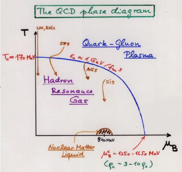
Figure 1.1: Phase diagram of QCD matter [6].

On the basis of thermodinamical considerations and of QCD calculations, strongly interacting matter is expected to exist in different states. Its behaviour, as a function of the baryonic chemical potential $\mu_{\rm B}$ (a measure of the baryonic density) and of the temperature $T$, is displayed in the phase diagram reported in Fig. 1.1. At low temperatures and for $\mu_{\rm B}\simeq m_{\rm p}\simeq 940\leavevmode\nobreak\ \mathrm{MeV}$, we have ordinary matter. Increasing the energy density of the system, by ‘compression’ (towards the right) or by ‘heating’ (upward), a hadronic gas phase is reached in which nucleons interact and form pions, excited states of the proton and of the neutron ($\Delta$ resonances) and other hadrons. If the energy density is further increased, the transition to the deconfined QGP phase is predicted: the density of partons (quarks and gluons) becomes so high that the confinement of quarks in hadrons vanishes.

The phase transition can be reached along different ‘paths’ on the $(\mu_{\rm B},\,T)$ plane. In the primordial Universe, the transition QGP-hadrons, from the deconfined to the confined phase, took place at $\mu_{\rm B}\approx 0$ (the global baryonic number was approximately zero) as a consequence of the expansion of the Universe and of the decrease of its temperature (path downward along the vertical axis) [7]. On the other hand, in the formation of neutron stars, the gravitational collapse causes an increase in the baryonic density at temperatures very close to zero (path towards the right along the horizontal axis) [7].

In heavy ion collisions, both temperature and density increase, possibly bringing the system to the phase transition. In the diagram in Fig. 1.1 the paths estimated for the fixed-target (SIS, AGS, SPS) and collider (RHIC, LHC) experiments are shown.

1.1.2 Lattice QCD results

Exploring from a theoretical point of view the qualitative features of the QGP and making quantitative predictions about its properties is the central goal of the numerical studies of strongly interacting matter thermodynamics within the framework of lattice QCD [8, 5].

Phase transitions are related to large-distance phenomena in a thermal medium. Because of the increasing strength of QCD interactions with the distance, such phenomena cannot be treated using perturbative methods. Lattice QCD provides a first-principle approach that allows to study large-distance aspects of QCD and to partially account for non-perturbative effects. However, at present, most calculations are limited by the fact that they do not include a finite baryo-chemical potential $\mu_{\rm B}$ (i.e. they assume a baryonic density equal to zero).

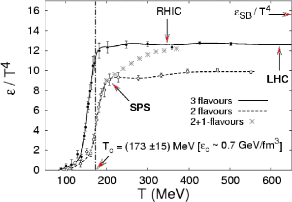
Figure 1.2: The energy density in lattice QCD with 2 and 3 light quarks and with 2 light plus 1 heavier (strange) quarks [5]. The calculation uses $\mu_{\rm B}=0$.

Results of a recent calculation of $\varepsilon/T^{4}$ are shown in Fig. 1.2, for 2- and 3-flavours QCD with light quarks and for 2 light plus 1 heavier (strange) quark (indicated by the stars) [5]. The latter case is likely to be the closest to the physically realized quark mass spectrum. The number of flavours and the masses of the quarks constitute the main uncertainties in the determination of the critical temperature and critical energy density. The critical temperature is estimated to be $T_{c}=(175\pm 15)\leavevmode\nobreak\ \mathrm{MeV}$ and the critical energy density $\varepsilon_{c}\simeq(6\pm 2)\,T_{c}^{4}\simeq(0.3$-$1.3)\leavevmode\nobreak\ \mathrm{GeV}/\mathrm{fm}^{3}$. Most of the uncertainty on $\varepsilon_{c}$ arises from the 10% uncertainty on $T_{c}$.

Although the transition is not a first order one (which would be characterized by a discontinuity of $\varepsilon$ at $T=T_{c}$), a large ‘jump’ of $\Delta\varepsilon/T_{c}^{4}\simeq 8$ in the energy density is observed in a temperature interval of only about $40\leavevmode\nobreak\ \mathrm{MeV}$ (for the 2-flavours calculation). Considering that the energy density of an equilibrated ideal gas of particles with $n_{\rm dof}$ degrees of freedom is

$$\varepsilon=n_{\rm dof}\,\frac{\pi^{2}}{30}\,T^{4},$$ (1.1)

the dramatic increase of $\varepsilon/T^{4}$ can be interpreted as due to the change of $n_{\rm dof}$ from 3 in the pion gas phase to 37 (with 2 flavours) in the deconfined phase, where the additional colour and quark flavour degrees of freedom are available.

1.2 Evidence for deconfinement in heavy ion collisions: the SPS programme

The desire to test this fascinating phase structure of strongly interacting matter first led to the fixed-target experiments at the AGS in Brookhaven (with $\sqrt{s_{\scriptscriptstyle{{\rm NN}}}}\simeq 5\leavevmode\nobreak\ \mathrm{GeV}$) and at the CERN-SPS (with $\sqrt{s_{\scriptscriptstyle{{\rm NN}}}}\simeq 17\leavevmode\nobreak\ \mathrm{GeV}$). In 1986/87, the programme started with lighter ion beams (O, S, Si) on heavy ion targets (Au, Pb), and in 1994/95, heavy ion beams followed, with Au–Au collisions at the AGS and Pb–Pb collisions at the SPS.

The evolution of a high-energy nucleus–nucleus collision is usually pictured in the form shown in Fig. 1.3 (left). After a rather short equilibration time $\tau_{0}\simeq 1\leavevmode\nobreak\ \mathrm{fm}/c$ (at the SPS), the presence of a thermalized medium is assumed, and for sufficiently-high energy densities, this medium would be in the quark–gluon plasma phase. Afterwards, as the expansion reduces the energy density, the system goes through a hadron gas phase and finally reaches the freeze-out, when the final state hadrons do not interact with each other anymore. The choice of heavy nuclei allows to maximize the energy and the volume in which the energy density is very large. The energy density at the time of local thermal equilibration can be determined using the Bjorken estimate [9]:

$$\varepsilon=\left(\frac{{\rm d}N_{\rm h}}{{\rm d}y}\right)_{y=0}\times\frac{w_{\rm h}}{\pi R_{\rm A}^{2}\tau_{0}},$$ (1.2)

where $({\rm d}N_{\rm h}/{\rm d}y)_{y=0}$ specifies the number of hadrons emitted per unit of rapidity at mid-rapidity and $w_{\rm h}$ their average energy in the direction transverse to the beam axis. The effective initial volume is determined in the transverse plane by the nuclear radius $R_{\rm A}$, and longitudinally by the formation time $\tau_{0}$ of the thermal medium.

Figure 1.3: Left: the expected evolution of a high-energy nuclear collision. Right: the energy density in Pb–Pb collisions at the SPS [10].

The energy density was measured in Pb–Pb collisions at $\sqrt{s_{\scriptscriptstyle{{\rm NN}}}}=17\leavevmode\nobreak\ \mathrm{GeV}$ at the SPS by the NA50 experiment [10]. In Fig. 1.3 (right) $\varepsilon$ is plotted as a function of the centrality of the collision, determined by the number of participant nucleons; it covers the range from 1 to $3.5\leavevmode\nobreak\ \mathrm{GeV}/\mathrm{fm}^{3}$. Lattice calculations, as already mentioned, give for the energy density at deconfinement, $\varepsilon(T_{c})$, values around or slightly below $1\leavevmode\nobreak\ \mathrm{GeV}/\mathrm{fm}^{3}$.

We describe here the two clearest pieces of evidence for the production of a deconfined medium in Pb–Pb collisions at the SPS. Both of these effects were predicted in the eighties:

• enhancement of the production of strange and multi-strange baryons (hyperons) with respect to the rates extrapolated from pp data (predicted by J. Rafelski and B. Müller in 1982 [11]);

• suppression of the production of the J$/\psi$ meson (the lowest $\mathrm{c\overline{c}}$ bound state), always with respect to the rates extrapolated from pp (predicted by T. Matsui and H. Satz in 1986 [12]).

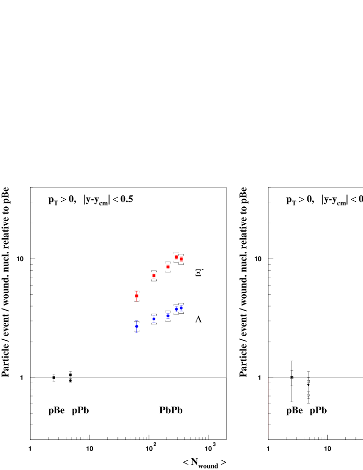
Figure 1.4: Strange baryon production in Pb–Pb per participant nucleon, normalized to the ratio from p–Be, as a function of the number of participant nucleons, as measured by NA57 at the SPS [13].

Figure 1.5: The ratio of J$/\psi$ to Drell-Yan production as a function of the transverse energy, measured by NA50, in Pb–Pb collisions at the SPS. The solid line indicates the extrapolation of the normal nuclear absorption inferred from pA collisions [10].

In the QGP, the chiral symmetry restoration decreases the threshold for the production of a $\rm s\overline{s}$ pair from twice the constituent mass of the s quark, $\approx 600\leavevmode\nobreak\ \mathrm{MeV}$, to twice the bare mass of the s quark, $\approx 300\leavevmode\nobreak\ \mathrm{MeV}$, which is less than half of the energy required to produce strange particles in hadronic interactions. In the QGP multi-strange baryons can be produced by statistical combination of strange (and non-strange) quarks, while in an hadronic gas they have to be produced through a chain of interactions that increase the strangeness content in steps of one unit. For this reason an hyperon enhancement growing with the strangeness content was indicated as a signal for QGP formation. This effect was, indeed, observed by the WA97/NA57 experiment: in Fig. 1.5 one can see that the production of strange and multi-strange baryons increases by 10 times and more (up to 20 times for the $\Omega$) in central Pb–Pb collisions in comparison to p–Be, where the QGP is not expected. As predicted, the enhancement $\mathcal{E}$ is increasing with the strangeness content: $\mathcal{E}(\Lambda)<\mathcal{E}(\Xi)<\mathcal{E}(\Omega)$.

Also the other historic predicted signal of deconfinement was clearly observed, by the NA50 experiment: in Fig. 1.5 the suppression of the J$/\psi$ particle with respect to the Drell-Yan process $q\overline{q}\to\ell^{+}\ell^{-}$, used as a reference, is shown as a function of the centrality, measured by the energy $E_{\rm T}$ emitted in the transverse plane, in Pb–Pb collisions. The line represents the expected trend of normal nuclear absorption extrapolated from proton–nucleus measurements. The additional suppression, clearly visible for central collision ($E_{\rm T}>60$-$80\leavevmode\nobreak\ \mathrm{GeV}$), is interpreted as due to the fact that, in the high colour-charge density environment of a QGP, the strong interaction between the two quarks of the $\mathrm{c\overline{c}}$ pair is screened and the formation of their bound state is consequently prevented.

The results of the SPS programme at CERN, and in particular the enhancement of strangeness production and the J$/\psi$ suppression, allowed to conclude that in Pb–Pb collisions at these energies a new state of matter is formed in which the effects of quark confinement appear to be removed [14, 15].

1.3 RHIC: focus on new observables

The Relativistic Heavy Ion Collider (RHIC) in Brookhaven began operation during summer 2000. With a factor 10 increase in the centre-of-mass energy with respect to the SPS, $\sqrt{s_{\scriptscriptstyle{{\rm NN}}}}$ up to $200\leavevmode\nobreak\ \mathrm{GeV}$, the produced collisions are expected to be well above the phase transition threshold. Moreover, in this energy regime, the so-called ‘hard processes’ —production of energetic partons ($E>3$-$5\leavevmode\nobreak\ \mathrm{GeV}$) out of the inelastic scattering of two partons from the colliding nuclei— have a significantly large cross section and they become experimentally accessible.

In this scenario, beyond the ‘traditional’ observables we have already introduced, the interesting phenomenon of in-medium parton energy loss [16, 17, 18], predicted for the first time by J.D. Bjorken in 1982 [16], can be addressed. Since the study of the sensitivity for the measurement of charm quarks energy loss at the LHC is one of the physics goals of this thesis work, a detailed description of the current theoretical view of this phenomenon will be given in Chapter 2. For the moment we will limit ourselves to a simplified description.

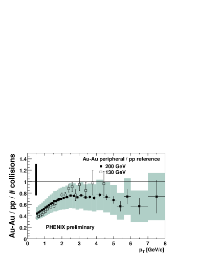
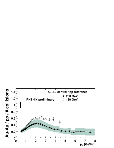
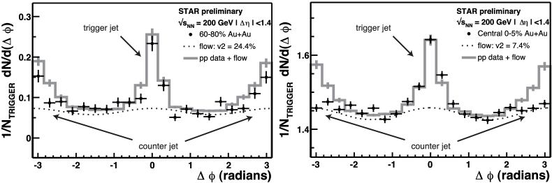
Figure 1.6: The ratio of transverse momentum distributions of charged hadrons in Au–Au collisions and pp collisions, scaled by the number of binary nucleon–nucleon collisions, at $\sqrt{s_{\scriptscriptstyle{{\rm NN}}}}=130$ and $200\leavevmode\nobreak\ \mathrm{GeV}$ [19].

Figure 1.7: Azimuthal correlations of charged particles relative to a high-$p_{\rm t}$ trigger particle for peripheral (left) and central (right) Au–Au collisions at $\sqrt{s_{\scriptscriptstyle{{\rm NN}}}}=200\leavevmode\nobreak\ \mathrm{GeV}$ [20].

Hard partons are produced at the early stage of the collision and they propagate through the medium formed in the collision. During this propagation they undergo QCD interactions with the gluons present in the medium and they lose energy. Such energy loss is not peculiar of a deconfined medium, but, quantitatively, it is strongly dependent on the nature and on the properties of the medium, being predicted to be much larger in the case of deconfinement. This last point can be intuitively understood considering that, if the parton travels through a deconfined medium, it finds much harder gluons to interact with than it would in a confined medium, where the gluons are constrained to carry only a very small fraction of the total hadron momentum, which is shared mainly among the valence quarks.

The measurement of high-$p_{\rm t}$ (projection of the momentum on the plane transverse to the beam line) particle production is addressed at RHIC mainly by the PHENIX and STAR experiments. The results, although still preliminary, have aroused considerable interest. Figure 1.7 reports the yield of charged hadrons measured by PHENIX [19] in peripheral (left) and central (right) Au–Au collisions at $\sqrt{s_{\scriptscriptstyle{{\rm NN}}}}=130$ and $200\leavevmode\nobreak\ \mathrm{GeV}$, divided by the yield in pp collisions (scaled to the same energy) and by the estimated number of binary nucleon–nucleon collisions. This ratio should be 1 at high $p_{\rm t}$ if no medium effects are present. In central collisions the yield of high-$p_{\rm t}$ ($8\leavevmode\nobreak\ \mathrm{GeV}/c$) hadrons is reduced of a factor 4 with respect to what expected for incoherent production in nucleon–nucleon collisions.

Another interesting result, obtained by STAR and PHENIX, is the gradual disappearing of the back-to-back azimuthal correlations of high-$p_{\rm t}$ particles with increasing collision centrality [20, 21]. In Fig. 1.7 the azimuthal correlations of charged particles with respect to a high-$p_{\rm t}$ trigger particle (black markers) are shown for peripheral (left) and central (right) collisions and compared with reference data from pp collisions (grey histogram): in central collisions the opposite-side ($\Delta\phi=\pm\pi$) correlation is strongly suppressed with respect to the pp and peripheral Au–Au cases. This effect suggests the absorption of one of the two jets (usually produced as back-to-back pairs) in the hot matter formed in central collisions.

The effects of leading particle and jet suppression shown in Figs. 1.7 and 1.7 are not observed in d–Au (deuteron–gold) collisions at $\sqrt{s_{\scriptscriptstyle{{\rm NN}}}}=200\leavevmode\nobreak\ \mathrm{GeV}$ [22, 23], where the formation of a dense medium is not expected.

1.4 LHC: study of ‘deeply deconfined’ matter

The Large Hadron Collider is scheduled to start operation in 2007. It will provide nuclear collisions at a centre-of-mass energy 30 times higher than at RHIC, opening a new era for the field, in which particle production will be dominated by hard processes, and the energy densities will possibly be high enough to treat the generated quark–gluon plasma as an ideal gas. These qualitatively new features will allow to address the task of the LHC heavy ion programme: a systematic study of the properties of the quark–gluon plasma state.

1.4.1 Systems, energies and expected multiplicity

The ion beams will be accelerated in the LHC at a momentum of $7\leavevmode\nobreak\ \mathrm{TeV}$ per unit of Z/A, where A and Z are the mass and atomic numbers of the ions, respectively. Thus, a generic ion $({\rm A,Z})$ will have momentum $p({\rm A,Z})={\rm(Z/A)}\,p^{\rm p}$, where $p^{\rm p}=7\leavevmode\nobreak\ \mathrm{TeV}$ is the momentum for a proton beam. The centre-of-mass (c.m.s.) energy per nucleon–nucleon pair in the collision of two generic nuclei ${\rm(A_{1},Z_{1})}$ and ${\rm(A_{2},Z_{2})}$ is:

$$\sqrt{s_{\scriptscriptstyle{{\rm NN}}}}=\sqrt{(E_{1}+E_{2})^{2}-(\vec{p}_{1}+\vec{p}_{2})^{2}}\simeq\sqrt{4\,p_{1}\,p_{2}}=\sqrt{\frac{\rm Z_{1}Z_{2}}{\rm A_{1}A_{2}}}\,14\leavevmode\nobreak\ \mathrm{TeV}.$$ (1.3)

The initial LHC running programme foresees [24]:

• Regular pp runs at $\sqrt{s}=14\leavevmode\nobreak\ \mathrm{TeV}$

• 1-2 years with Pb–Pb runs at $\sqrt{s_{\scriptscriptstyle{{\rm NN}}}}=5.5\leavevmode\nobreak\ \mathrm{TeV}$

• 1 year with p–Pb runs at $\sqrt{s_{\scriptscriptstyle{{\rm NN}}}}=8.8\leavevmode\nobreak\ \mathrm{TeV}$ (or d–Pb or $\alpha$–Pb)

• 1-2 years with Ar–Ar at $\sqrt{s_{\scriptscriptstyle{{\rm NN}}}}=6.3\leavevmode\nobreak\ \mathrm{TeV}$

As we have seen for SPS and RHIC, the proton–proton and proton–nucleus runs are mandatory for comparison of the results obtained with Pb–Pb collisions; we will detail this point during the discussion on the hard probes in Section 1.5.2. The runs with lighter ions (e.g. argon) will allow to vary the energy density and the volume of the produced system. At least for what concerns the hard observables, the fact of having different c.m.s. energies for the different systems is not expected to introduce large uncertainties in the comparisons, because perturbative QCD (pQCD) calculations can be used quite safely for the extrapolation to different energies (for example to scale the results measured in pp at $14\leavevmode\nobreak\ \mathrm{TeV}$ to the energy of Pb–Pb, $5.5\leavevmode\nobreak\ \mathrm{TeV}$). In Chapter 7 a strategy for this extrapolation will be presented and discussed, for charm production.

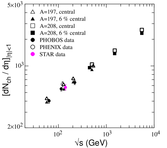
Figure 1.8: Charged multiplicity per unit of pseudorapidity ${\rm d}N_{\rm ch}/{\rm d}\eta$ ($\simeq{\rm d}N_{\rm ch}/{\rm d}y$, at $y=0$) in AA collisions. Square and triangle markers are model predictions [25]. Circle markers are measurements at RHIC.

The most important global observable is the average charged particle multiplicity per rapidity unit (${\rm d}N_{\rm ch}/{\rm d}y$) in central Pb–Pb collisions. On the theoretical side, since it is related to the attained energy density (see Bjorken’s formula in equation (1.2)), it enters the calculation of most other observables. On the experimental side, the particle multiplicity fixes the main unknown in the detector performance and the accuracy with which many observables can be measured.

There is no first principle calculation of ${\rm d}N_{\rm ch}/{\rm d}y$ starting from the QCD Lagrangian, since particle production is dominated by soft non-perturbative QCD. Therefore, the large variety of available models of heavy ion collisions gives a wide range of predicted multiplicities. Before RHIC, the predictions for the LHC reached up to more than 8000 charged particles per unit of rapidity. The multiplicity measured at RHIC, ${\rm d}N_{\rm ch}/{\rm d}y\simeq 650$ at $\sqrt{s_{\scriptscriptstyle{{\rm NN}}}}=200\leavevmode\nobreak\ \mathrm{GeV}$, is about a factor 2 lower than what was predicted by most models. In the light of this result, the multiplicity at the LHC is not expected to be larger than $3000$-$4000$ charged particles per unit of rapidity. Figure 1.8 presents the result of a model [25] that well reproduces the multiplicities measured at RHIC. It predicts ${\rm d}N_{\rm ch}/{\rm d}y\simeq{\rm d}N_{\rm ch}/{\rm d}\eta\simeq 2500$ for central Pb–Pb at the LHC .

Since this thesis work started before the first results from RHIC were available, the simulations were performed using ${\rm d}N_{\rm ch}/{\rm d}y=6000$. However, this (probably) over-estimated value provides a safety factor on the obtained results, which were, for completeness, extrapolated also to ${\rm d}N_{\rm ch}/{\rm d}y=3000$.

1.4.2 Why ‘deep deconfinement’?

Starting from the estimates of the charged multiplicity many parameters of the medium produced in the collision can be inferred. Table 1.1 presents a comparison of the most relevant parameters for SPS, RHIC and LHC energies [26].

At the LHC, the high energy in the collision centre of mass is expected to determine a large energy density and an initial temperature at least a factor 2 larger than at RHIC. This high initial temperature extends also the life-time and the volume of the deconfined medium, since it has to expand while cooling down to the freeze-out temperature, which is $\approx 170\leavevmode\nobreak\ \mathrm{MeV}$ (it is independent of $\sqrt{s}$, above the SPS energy). In addition, the large expected number of gluons favours energy and momentum exchanges, thus considerably reducing the time needed for the thermal equilibration of the medium. To summarize, the LHC will produce hotter, larger and longer-living ‘drops’ of QCD plasma than the present heavy ion facilities.

The key advantage in this new ‘deep deconfinement’ scenario is that the quark–gluon plasma studied by the LHC experiments will be much more similar to the quark–gluon plasma that can be investigated from a theoretical point of view by means of lattice QCD.

As mentioned, lattice calculations are mostly performed for a baryon-free system ($\mu_{\rm B}=0$). In general, $\mu_{\rm B}=0$ is not valid for heavy ion collisions, since the two colliding nuclei carry a total baryon number equal to twice their mass number. However, the baryon content of the system after the collision is expected to be concentrated rather near the rapidity of the two colliding nuclei. Therefore, the larger the rapidity of the beams, with respect to their center of mass, the lower the baryo-chemical potential in the central rapidity region. The rapidities of the beams at SPS, RHIC and LHC are 2.9, 5.3 and 8.6, respectively. Clearly, the LHC is expected to be much more baryon-free than RHIC and SPS and, thus, closer to the conditions simulated in lattice QCD.

Table 1.1: Comparison of the parameters characterizing central nucleus–nucleus collisions at different energy regimes [26].

Parameter		SPS	RHIC	LHC
$\sqrt{s_{\scriptscriptstyle{{\rm NN}}}}$	[GeV]	17	200	5500
d$N_{\rm gluons}/$d$y$		$\simeq 450$	$\simeq 1200$	$\simeq 5000$
${\rm d}N_{\rm ch}/{\rm d}y$		400	650	$\simeq 3000$
Initial temperature	[MeV]	200	350	$>600$
Energy density	[$\mathrm{GeV}/\mathrm{fm}^{3}$]	3	25	120
Freeze-out volume	[$\mathrm{fm}^{3}$]	few $10^{3}$	few $10^{4}$	few $10^{5}$
Life-time	[$\mathrm{fm}/c$]	$<2$	$2$-$4$	$>10$

In addition to this effect, also the higher temperature predicted for the LHC favours the comparison with theory. This point can be better understood by going back to the lattice results for $\varepsilon/T^{4}$ (Fig. 1.2). If we now concentrate on the result obtained with 2+1 flavours, 2 light quarks plus a heavier one, we notice that $\varepsilon/T^{4}$ continues to rise for $T>T_{c}$, indicating that significant non-perturbative effects, not fully accounted for in the lattice formalism, are to be expected at least up to temperatures $T\simeq(2$-$3)\,T_{c}$. In Ref. [27] the strong coupling constant in this range is estimated as

$$\alpha_{s}(T)=\frac{4\pi}{18\,\ln(5\,T/\Lambda_{\rm QCD})}=\left\{\begin{array}[]{ll}0.43&{\rm for}\leavevmode\nobreak\ T=T_{c}\\ 0.3&{\rm for}\leavevmode\nobreak\ T=2\,T_{c}\\ 0.23&{\rm for}\leavevmode\nobreak\ T=4\,T_{c}\\ \end{array}\right.$$ (1.4)

using the fact that the QCD scaling constant $\Lambda_{\rm QCD}$ is of the same order of magnitude as $T_{c}$, $\approx 200\leavevmode\nobreak\ \mathrm{MeV}$. These values confirm that non-perturbative effects are larger in the range $T<2\,T_{c}$.

The conditions produced in heavy ion collisions at SPS and RHIC are contained in this range ($T_{\rm SPS}\approx 1.2\times T_{c}$ and $T_{\rm RHIC}\approx 2\times T_{c}$), meaning that in these cases the comparison of experimentally determined quantities, such as temperature or energy density, to lattice QCD calculations is not fully reliable. With an initial temperature of $\sim(4$-$5)\,T_{c}$ predicted for central Pb–Pb collisions at $\sqrt{s_{\scriptscriptstyle{{\rm NN}}}}=5.5\leavevmode\nobreak\ \mathrm{TeV}$, the LHC will provide closer-to-ideal conditions (i.e. with smaller non-perturbative effects), allowing a direct comparison to the theoretical calculations. In this sense, the regime that will be realized at the LHC may be defined as ‘deep deconfinement’.

1.5 Novel aspects of heavy ion physics at the LHC

Heavy ion collisions at the LHC access not only a quantitatively different regime of much higher energy density but also a qualitatively new regime, mainly because:

1. High-density parton distributions are expected to dominate particle production. The number of low-energy partons (mainly gluons) in the two colliding nuclei is, therefore, expected to be so large as to produce a significant shadowing effect (described later) that suppresses the inelastic scatterings with low momentum transfer.

2. Hard processes should contribute significantly to the total AA cross section. The hard probes are at the LHC an ideal experimental tool for a detailed characterization of the QGP medium.

In the following we discuss these two aspects.

1.5.1 Low-$x$ parton distribution functions

In the inelastic collision of a proton (or, more generally, nucleon) with a particle, the Bjorken $x$ variable is defined as the fraction of the proton momentum carried by the parton that enters the hard scattering process. The distribution of $x$ for a given parton type (e.g. gluon, valence quark, sea quark) is called Parton Distribution Function (PDF) and it gives the probability to pick up a parton with momentum fraction $x$ from the proton. The main experimental knowledge on the proton PDFs comes from Deep Inelastic Scattering (DIS) data, in particular from HERA data for the small-$x$ region. Several groups (MRST [28], CTEQ [29], GRV [30]) have developed parameterizations of these data in the framework of DGLAP (Dokshitzer-Gribov-Lipatov, Altarelli-Parisi) QCD evolution [31]. An example of proton PDFs will be shown at the end of the next paragraph.

Accessible $x$ range

The LHC will allow to probe the parton distribution functions of the nucleon and, in the case of proton–nucleus and nucleus–nucleus collisions, also their modifications in the nucleus, down to unprecedented low values of $x$. In this paragraph we compare the values of $x$ corresponding to the production of a $\mathrm{c\overline{c}}$ pair at SPS, RHIC and LHC energies and we estimate the $x$ range that can be accessed with ALICE for what concerns heavy flavour production. This information is particularly valuable because the charm and beauty production cross sections at the LHC are significantly affected by parton dynamics in the small-$x$ region, as we will see in Chapter 3. Therefore, the measurement of heavy flavour production may provide information on the nuclear parton densities.

We can consider the simple case of the production of a heavy quark pair, $Q\overline{Q}$, through the leading order gluon–gluon fusion process $gg\to Q\overline{Q}$ in the collision of two ions $({\rm A}_{1},{\rm Z}_{1})$ and $({\rm A}_{2},{\rm Z}_{2})$. The $x$ range actually probed depends on the value of the c.m.s. energy per nucleon pair $\sqrt{s_{\scriptscriptstyle{{\rm NN}}}}$, on the invariant mass $M_{Q\overline{Q}}$ of the $Q\overline{Q}$ pair produced in the hard scattering and on the rapidity $y_{Q\overline{Q}}$ of the pair. If the parton intrinsic transverse momentum in the nucleon is neglected, the four-momenta of the two incoming gluons are $(x_{1},0,0,x_{1})\cdot({\rm Z_{1}/A_{1}})\,\sqrt{s_{\rm pp}}/2$ and $(x_{2},0,0,-x_{2})\cdot({\rm Z_{2}/A_{2}})\,\sqrt{s_{\rm pp}}/2$, where $x_{1}$ and $x_{2}$ are the momentum fractions carried by the gluons, and $\sqrt{s_{\rm pp}}$ is the c.m.s. energy for pp collisions ($14\leavevmode\nobreak\ \mathrm{TeV}$ at the LHC). The square of the invariant mass of the $Q\overline{Q}$ pair is given by:

$$M^{2}_{Q\overline{Q}}=\hat{s}=x_{1}\,x_{2}\,s_{\scriptscriptstyle\rm NN}=x_{1}\,\frac{{\rm Z}_{1}}{{\rm A}_{1}}\,x_{2}\,\frac{{\rm Z}_{2}}{{\rm A}_{2}}\,s_{\rm pp};$$ (1.5)

and its longitudinal rapidity in the laboratory is:

$$y_{Q\overline{Q}}=\frac{1}{2}\ln\left[\frac{E+p_{z}}{E-p_{z}}\right]=\frac{1}{2}\ln\left[\frac{x_{1}}{x_{2}}\cdot\frac{{\rm Z}_{1}\,{\rm A}_{2}}{{\rm Z}_{2}\,{\rm A}_{1}}\right].$$ (1.6)

From these two relations we can derive the dependence of $x_{1}$ and $x_{2}$ on colliding system, $M_{Q\overline{Q}}$ and $y_{Q\overline{Q}}$:

$$x_{1}=\frac{{\rm A}_{1}}{{\rm Z}_{1}}\cdot\frac{M_{Q\overline{Q}}}{\sqrt{s_{\rm pp}}}\exp\left({+y_{Q\overline{Q}}}\right)\leavevmode\nobreak\ \leavevmode\nobreak\ \leavevmode\nobreak\ \leavevmode\nobreak\ \leavevmode\nobreak\ \leavevmode\nobreak\ \leavevmode\nobreak\ \leavevmode\nobreak\ \leavevmode\nobreak\ \leavevmode\nobreak\ \leavevmode\nobreak\ \leavevmode\nobreak\ \leavevmode\nobreak\ \leavevmode\nobreak\ \leavevmode\nobreak\ \leavevmode\nobreak\ x_{2}=\frac{{\rm A}_{2}}{{\rm Z}_{2}}\cdot\frac{M_{Q\overline{Q}}}{\sqrt{s_{\rm pp}}}\exp\left({-y_{Q\overline{Q}}}\right);$$ (1.7)

which simplifies to

$$x_{1}=\frac{M_{Q\overline{Q}}}{\sqrt{s_{\scriptscriptstyle{{\rm NN}}}}}\exp\left({+y_{Q\overline{Q}}}\right)\leavevmode\nobreak\ \leavevmode\nobreak\ \leavevmode\nobreak\ \leavevmode\nobreak\ \leavevmode\nobreak\ \leavevmode\nobreak\ \leavevmode\nobreak\ \leavevmode\nobreak\ \leavevmode\nobreak\ \leavevmode\nobreak\ \leavevmode\nobreak\ \leavevmode\nobreak\ \leavevmode\nobreak\ \leavevmode\nobreak\ \leavevmode\nobreak\ \leavevmode\nobreak\ x_{2}=\frac{M_{Q\overline{Q}}}{\sqrt{s_{\scriptscriptstyle{{\rm NN}}}}}\exp\left({-y_{Q\overline{Q}}}\right)$$ (1.8)

for a symmetric colliding system ($\rm A_{1}=A_{2}$, $\rm Z_{1}=Z_{2}$).

At central rapidities we have $x_{1}\simeq x_{2}$ and their magnitude is determined by the ratio of the pair invariant mass to the c.m.s. energy. For production at the threshold ($M_{\rm\scriptstyle{c\overline{c}}}=2\,m_{\rm c}\simeq 2.4$ GeV, $M_{\rm\scriptstyle{b\overline{b}}}=2\,m_{\rm b}\simeq 9$ GeV) we obtain what reported in Table 1.2. The $x$ regime relevant to charm production at the LHC ($\sim 10^{-4}$) is about 2 orders of magnitude lower than at RHIC and 3 orders of magnitude lower than at the SPS.

Table 1.2: Bjorken $x$ values corresponding to charm and beauty production at threshold at central rapidity.

Machine	SPS	RHIC	LHC	LHC
System	Pb–Pb	Au–Au	Pb–Pb	pp
$\sqrt{s_{\scriptscriptstyle{{\rm NN}}}}$	17 GeV	200 GeV	5.5 TeV	14 TeV
$\mathrm{c\overline{c}}$	$x\simeq 10^{-1}$	$x\simeq 10^{-2}$	$x\simeq 4\cdot 10^{-4}$	$x\simeq 2\cdot 10^{-4}$
$\mathrm{b\overline{b}}$	–	–	$x\simeq 2\cdot 10^{-3}$	$x\simeq 6\cdot 10^{-4}$

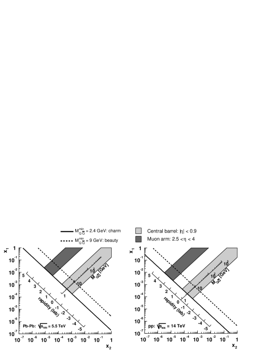
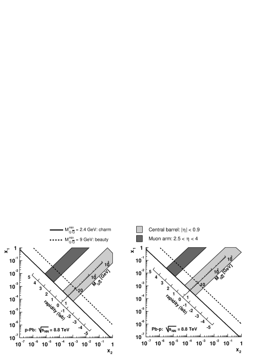
Figure 1.9: ALICE acceptance in the ($x_{1}$, $x_{2}$) plane for heavy flavours in Pb–Pb (left) and in pp (right). The figure is explained in detail in the text.

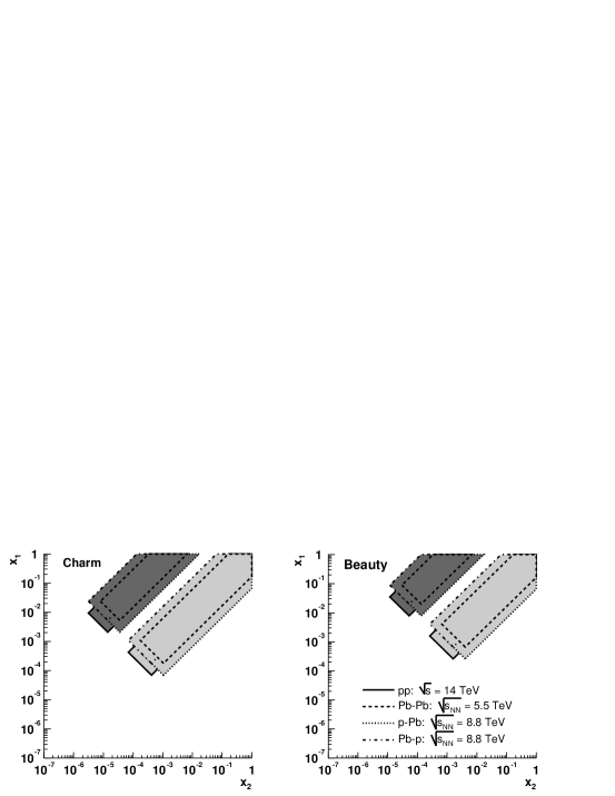
Figure 1.10: ALICE acceptance in the ($x_{1}$, $x_{2}$) plane for heavy flavours in p–Pb (left) and in Pb–p (right).

Figure 1.11: ALICE acceptance in the ($x_{1}$, $x_{2}$) plane for charm (left) and beauty (right) in pp, Pb–Pb, p–Pb and Pb–p.

Because of its lower mass, charm allows to probe lower $x$ values than beauty. The capability to measure charm and beauty particles in the forward rapidity region ($y\simeq 4$) would give access to $x$ regimes about 2 orders of magnitude lower, down to $x\sim 10^{-6}$.

In Fig. 1.11 we show the regions of the ($x_{1}$, $x_{2}$) plane covered for charm and beauty by the ALICE acceptance, in Pb–Pb at 5.5 TeV and in pp at 14 TeV. In this plane the points with constant invariant mass lie on hyperbolae ($x_{1}=M^{2}_{Q\overline{Q}}/(x_{2}\,s_{\scriptscriptstyle\rm NN})$), straight lines in the log-log scale: we show those corresponding to the production of $\mathrm{c\overline{c}}$ and $\mathrm{b\overline{b}}$ pairs at the threshold; the points with constant rapidity lie on straight lines ($x_{1}=x_{2}\exp(+2\,y_{Q\overline{Q}})$). The shadowed regions show the acceptance of the ALICE central barrel, covering the pseudorapidity range $|\eta|<0.9$, and of the muon arm, $2.5<\eta<4$ (the ALICE experimental layout will be described in Chapter 4).

In the case of asymmetric collisions, e.g. p–Pb and Pb–p, we have a rapidity shift: the centre of mass moves with a longitudinal rapidity

$$y_{\rm c.m.}=\frac{1}{2}\ln\left(\frac{\rm Z_{1}A_{2}}{\rm Z_{2}A_{1}}\right),$$ (1.9)

obtained from equation (1.6) for $x_{1}=x_{2}$. The rapidity window covered by the experiment is consequently shifted by

$$\Delta y=y_{\rm lab.\leavevmode\nobreak\ system}-y_{\rm c.m.\leavevmode\nobreak\ system}=y_{\rm c.m.},$$ (1.10)

corresponding to $+0.47$ ($-0.47$) for p–Pb (Pb–p) collisions. Therefore, running with both p–Pb and Pb–p will allow to cover the largest interval in $x$. Figure 1.11 shows the acceptances for p–Pb and Pb–p, while in Fig. 1.11 the coverages in pp, Pb–Pb, p–Pb and Pb–p are compared for charm (left) and beauty (right).

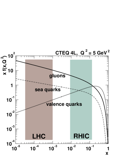
Figure 1.12: Parton distribution functions in the proton, in the CTEQ 4L parameterization, for $Q^{2}=5\leavevmode\nobreak\ \mathrm{GeV}^{2}$.

These figures are meant to give a first idea of the regimes accessible at ALICE; the simple relations for the leading order case were used, the ALICE rapidity acceptance cuts were applied to the rapidity of the $Q\overline{Q}$ pair, and not to that of the particles which are actually detected. In addition, no minimum $p_{\rm t}$ cuts were accounted for: such cuts will increase the minimum accessible value of $M_{Q\overline{Q}}$, thus increasing also the minimum accessible $x$. These approximations, however, are not too drastic, since there is a very strong correlation in rapidity between the initial $Q\overline{Q}$ pair and the heavy flavour particles it produces and the minimum $p_{\rm t}$ cut will be quite low (lower than the mass of the hadron) for most of the channels studied at ALICE. This last point was demonstrated within this thesis work for the specific case of open charm measurements at central rapidity (Chapter 6).

The parton distribution functions $x\,f(x,Q^{2})$ in the proton, in the CTEQ 4L parameterization, are shown in Fig. 1.12. $Q^{2}$ is the virtuality, or QCD scale (in the case of the leading order heavy flavour production considered in this paragraph, $Q^{2}=M^{2}_{Q\overline{Q}}=s\,x_{1}\,x_{2}$). In the figure the value $Q^{2}=5\leavevmode\nobreak\ \mathrm{GeV}^{2}$, corresponding to $\mathrm{c\overline{c}}$ production at threshold, is used. The regions in $x$ covered, at central rapidities, at RHIC and LHC are indicated by the shaded areas.

Nuclear shadowing effect

The extension of the $x$ range down to $\sim 10^{-4}$ at the LHC means, in a very simplified picture, that a large-$x$ parton in one of the two colliding Pb nuclei ‘sees’ the other incoming nucleus as a superposition of $\sim{\rm A}\times 1/10^{-4}\sim 10^{6}$ gluons. These gluons are so many that the lower-momentum ones tend to merge together: two gluons with momentum fractions $x_{1}$ and $x_{2}$ merge in a gluon with momentum fraction $x_{1}+x_{2}$ ($g_{x_{1}}g_{x_{2}}\to g_{x_{1}+x_{2}}$). As a consequence of this ‘migration towards larger $x$’, that does not affect only gluons but all partons, the nuclear parton densities are depleted in the small-$x$ region (and slightly enhanced in the large-$x$ region) with respect to the proton parton densities.

This phenomenon is known as nuclear shadowing effect and it has been experimentally studied in electron–nucleus DIS in the range $5\cdot 10^{-3}<x<1$ [32]. However, no data are available in the $x$ range covered by the LHC and the existing data provide only weak constraints for the gluon PDFs, which do not enter the measured structure functions at leading order. Only two groups (EKS [33] and HKM [34]) have used the same approach as in the case of the proton to obtain a parameterization (and extrapolation to low $x$) of the nuclear-modified PDFs. Nuclear PDFs were also computed in several other models which tend to disagree where no experimental constraints are available.

The situation is summarized in Fig. 1.13 that shows the results of the different models for the ratio of the gluon distribution in a Pb nucleus over the gluon distribution in a proton:

$$R_{g}(x,Q^{2})=\frac{g^{\rm Pb}(x,Q^{2})}{g^{\rm p}(x,Q^{2})}.$$ (1.11)

In the figure the value $Q^{2}=5\leavevmode\nobreak\ \mathrm{GeV}^{2}$, corresponding to $\mathrm{c\overline{c}}$ production at threshold, is used.

Figure 1.13: Ratio of the gluon distribution function for Pb to the one for proton using different models at $Q^{2}=5\leavevmode\nobreak\ \mathrm{GeV}^{2}$.

The predictions for the gluon shadowing at the LHC ($R_{g}(x\sim 10^{-4})$) range from 30% to 90%. This large uncertainty will be reduced in the future by (a) more data in DIS with nuclei, (b) the pA data collected at RHIC and, most important, (c) the measurements of charm and beauty production in p–Pb at the LHC.

For the present work, we used the EKS98 [33] parameterization since it is the one which includes most constraints from DIS data. It gives $R_{g}(x\sim 10^{-4})\simeq 65\%$; in Chapter 3 we will see that this determines a reduction of 35% for the charm cross section per nucleon–nucleon collision in Pb–Pb with respect to pp collisions at the same c.m.s. energy.

1.5.2 Hard partons: probes of the QGP medium

“Qualitatively, in minimum-bias Pb–Pb (or Au–Au) collisions, SPS is 98% soft and 2% hard, RHIC is 50% soft and 50% hard and LHC is 2% soft and 98% hard” (K. Kajantie [27]). This means that at the LHC practically in all minimum-bias events (no centrality selection applied) high-$p_{\rm t}$ partons are expected to be produced in scattering processes involving a hard perturbative scale $Q\gg\Lambda_{\rm QCD}\simeq 200\leavevmode\nobreak\ \mathrm{MeV}$.

We give two examples of this significant qualitative difference of the LHC with respect to SPS and RHIC. The perturbative QCD (pQCD) results for the differential cross sections for charged hadrons and neutral pions at SPS, RHIC and LHC energies are shown in Fig. 1.14. The estimated yields for charm and beauty production are reported in Table 1.3: the $\mathrm{c\overline{c}}$ and $\mathrm{b\overline{b}}$ yields are expected to be 10 and 100 times larger, respectively, at the LHC than at RHIC.

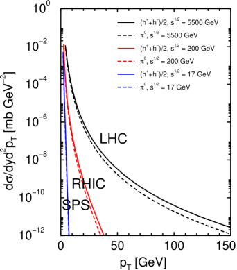
Figure 1.14: The predicted leading order (LO) differential cross section for neutral pion and charged hadron production is shown for pp collisions at $\sqrt{s}=17,\leavevmode\nobreak\ 200,\leavevmode\nobreak\ 5500\leavevmode\nobreak\ \mathrm{GeV}$.

Table 1.3: Charm and beauty production yields (per event) estimated for central Pb–Pb collisions at $\sqrt{s_{\scriptscriptstyle{{\rm NN}}}}=17,\leavevmode\nobreak\ 200,\leavevmode\nobreak\ 5500\leavevmode\nobreak\ \mathrm{GeV}$.

$\sqrt{s}$	SPS, 17 GeV	RHIC, 200 GeV	LHC, 5.5 TeV
$N(\mbox{$\mathrm{c\overline{c}}$})$	0.2	10	120
$N(\mbox{$\mathrm{b\overline{b}}$})$	–	0.05	5

Initial state and final state effects

In the absence of nuclear and medium effects, a nucleus–nucleus collision can be considered as a superposition of independent nucleon–nucleon collisions. Thus, the cross section for hard processes should scale from pp to AA proportionally to the number of inelastic nucleon–nucleon collisions (binary scaling).

The effects that can modify this simple scaling are usually divided in two classes:

• initial state effects, such as nuclear shadowing (described in Section 1.5.1), that affect the hard cross section in a way which depends on the size and energy of the colliding nuclei, but not on the medium formed in the collision;

• final state effects, induced by the medium, that can change the yields and/or the kinematic distributions (e.g. $p_{\rm t}$ and rapidity) of the produced hard partons; a typical example is the partonic energy loss; these final state effects are not correlated to the initial state effects, they depend strongly on the properties (gluon density, temperature and volume) of the medium and they can therefore provide information on such properties.

Initial state effects can be studied using pp and proton–nucleus collisions and then reliably extrapolated to nucleus–nucleus. If a quark–gluon plasma is formed in AA collisions, the final state effects will be significantly stronger than what is expected by an extrapolation from pA.

Why hard partons are good probes

Primary hard quarks and gluons are very well suited to probe the medium for three main reasons:

1. They are produced in the early stage of the collision in primary partonic scatterings, $gg\to gg$ or $gg\to q\overline{q}$, with large virtuality $Q$ and, thus, on temporal and spatial scales, $\Delta\tau\sim 1/Q$ and $\Delta r\sim 1/Q$, which are sufficiently small for the production to be unaffected by the properties of the medium (i.e. by final state effects).

2. Given the large virtuality, the production cross sections can be reliably calculated with the perturbative approach of pQCD. In fact, since

   $$\alpha_{s}(Q^{2})\propto\frac{1}{\ln(Q^{2}/\Lambda^{2}_{\rm QCD})},$$

   in an expansion of the cross sections in powers of $\alpha_{s}$, for large values of $Q^{2}$, the higher-order terms (in general higher than next-to-leading order, $\mathcal{O}(\alpha_{s}^{3})$) are small and can be neglected.
   In this way, as already mentioned, one can safely use pQCD for the energy interpolations needed to compare pp, pA and AA and disentangle initial and final state effects.

3. They are expected to be significantly attenuated, through the QCD energy loss mechanisms, when they propagate in the medium. The current theoretical understanding of these mechanisms and of the magnitude of the energy loss are extensively covered in the next chapter, with particular focus on the predictions for charm quarks.

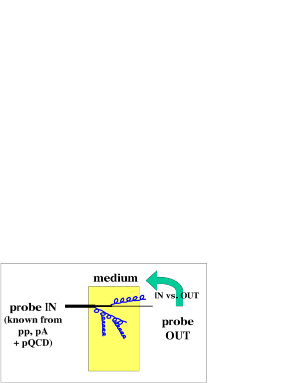
Figure 1.15: Schematic representation of how hard probes can be used to investigate the properties of the medium.

Figure 1.15 shows a schematic view of how hard probes ‘work’: the input (yields and $p_{\rm t}$ distributions) is known from the measurements carried out in pp (and pA) interpolated to the AA energy by pQCD and scaled according to the number of binary nucleon–nucleon collisions. The comparison of the output, measured ‘after the medium’, to the input allows to gain information on the medium itself.

Chapter 2 Charm in heavy ion collisions

Heavy quarks are sensitive probes of the medium produced in nucleus–nucleus collisions. In fact, they present all the features listed at the end of the previous chapter.

1. Initial production not affected by final state effects: the minimum value of the virtuality $Q_{\rm min}=2\,m_{Q}$ in the production of a $Q\overline{Q}$ pair implies very small space-time scales of $\sim 1/(2\,m_{Q})\simeq 1/2.4\leavevmode\nobreak\ \mathrm{GeV}^{-1}\simeq 0.1\leavevmode\nobreak\ \mathrm{fm}$ (for charm), to be compared to the expected life-time of the QGP phase at the LHC, $>10\leavevmode\nobreak\ \mathrm{fm}$. Thus, the initially-produced heavy quarks experience the full collision history.

2. Predictivity by pQCD: this is another consequence of the large mass (compared to $\Lambda_{\rm QCD}$). In Section 2.1 we show the main production channels and the general lines followed for the cross section calculations in proton–proton collisions.

3. Strong nuclear effects: both initial and final state effects are expected to enter in the production and propagation of heavy quarks, respectively; consequently, they are information-rich probes. Such effects are summarized in Section 2.2. In particular, the study of the energy loss of heavy quarks at the LHC is very interesting, because of the prediction of a significant mass-dependence of the effect (Section 2.3).

In the present work we concentrate on charm physics because (a) the production cross section is expected to be a factor $\simeq 20$ larger for charm than for beauty and (b) charm mesons can be exclusively reconstructed even in Pb–Pb collisions at the LHC via the decay channel ${\rm D^{0}\to K^{-}\pi^{+}}$ (as we will show in Chapter 6), while the feasibility of the exclusive reconstruction of beauty particles, e.g. via ${\rm B^{0}\to K_{S}^{0}\,J/\psi}$, is still unclear. For these two reasons charm can be studied with better precision (smaller statistical uncertainties) and accuracy (smaller systematic uncertainties) than beauty.

Experimentally, charm production was extensively studied in pA collisions, for energies up to $\sqrt{s_{\scriptscriptstyle{{\rm NN}}}}\approx 40\leavevmode\nobreak\ \mathrm{GeV}$. In AA collisions the present knowledge (from SPS and RHIC) is quite poor, since up to now no dedicated experiments were performed. The situation is summarized in Section 2.4.

At the end of the chapter we introduce the strategy aimed at the measurement and study of charm production in the LHC heavy ion programme with the ALICE detector (Section 2.5). The evaluation of the feasibility of this strategy and the attainable sensitivity for the study of charm physics are the central subject of this thesis work.

2.1 Heavy quark production in pQCD

At LHC energies, heavy quarks are produced, at leading order, via pair creation by gluon–gluon fusion ($gg\to Q\overline{Q}$), mostly, and $q\overline{q}$ annihilation ($q\overline{q}\to Q\overline{Q}$). At next-to-leading order more complicated topologies are included. Usually, the processes are classified according to the number of heavy quarks in the final state of the hard process, defined as the process with the highest virtuality (i.e. highest invariant mass of the outgoing parton pair, as defined in equation (1.5)). There are basically three classes of processes:

pair creation:

the hard process is one of the leading order graphs ($gg\rightarrow Q\overline{Q}$, $q\overline{q}\rightarrow Q\overline{Q}$); its final state contains two heavy quarks;

flavour excitation:

an incoming heavy quark is put on mass shell by scattering on a parton of the other beam: $qQ\rightarrow qQ$ or $gQ\rightarrow gQ$; the incoming heavy quark must come from a $g\rightarrow Q\overline{Q}$ splitting in the PDF of the proton; this process is characterized by one heavy quark in the final state of the hard scattering;

gluon splitting:

no heavy flavour is involved in the hard scattering, but a $Q\overline{Q}$ pair is produced in the final state from a $g\rightarrow Q\overline{Q}$ branching.

Figure 2.1 shows some topologies belonging to the processes specified above.

Figure 2.1: Some of the processes defined as pair creation, flavour excitation and gluon splitting. The thick lines correspond to the hard process.

At any order, the partonic cross section can be expressed in terms of the dimensionless scaling functions $F^{(k,l)}_{ij}$ that depend only on the variable $\xi$ [35]

$$\hat{\sigma}_{ij}(\hat{s},m_{Q}^{2},\mu_{R},\mu_{F})=\frac{\alpha_{s}^{2}(\mu_{F})}{m_{Q}^{2}}\sum_{k=0}^{\infty}(4\pi\alpha_{s}(\mu_{F}))^{k}\sum_{l=0}^{k}F_{ij}^{(k,l)}(\xi)\ln^{l}\left(\frac{\mu_{R}^{2}}{m_{Q}^{2}}\right),$$ (2.1)

where $\hat{s}$ is the partonic centre-of-mass energy squared for two partons $i$ and $j$ carrying momentum fractions $x_{i}$ and $x_{j}$ ($\hat{s}=x_{i}\,x_{j}\,s$), $m_{Q}$ is the heavy quark mass, $\mu_{F}$ and $\mu_{R}$ are the factorization and renormalization scales, respectively, and $\xi=\hat{s}/4m_{Q}^{2}-1$. The cross section is calculated as an expansion in powers of $\alpha_{s}$ with $k=0$ corresponding to the LO cross section. The first correction, $k=1$, corresponds to the NLO cross section. The complete calculation only exists up to NLO. However, as already mentioned, given the large value of $m_{Q}$, the corrections above NLO are expected to be small.

The total hadronic cross section in pp collisions is obtained by convoluting the total partonic cross section with the parton distribution functions $f_{i}^{\rm p}|_{i=q,\overline{q},g}$ of the initial protons (factorization),

$$\sigma^{\scriptstyle Q\overline{Q}}_{\rm pp}=\sum_{i,j=q,\overline{q},g}\int_{4m_{Q}^{2}/s}^{1}\frac{{\rm d}\tau}{\tau}\delta(x_{i}x_{j}-\tau)\,f_{i}^{\rm p}(x_{i},\mu_{F})\,f_{j}^{\rm p}(x_{j},\mu_{F})\,\hat{\sigma}_{ij}(\tau s,m_{Q}^{2},\mu_{R},\mu_{F}),$$ (2.2)

where $\tau=\hat{s}/s$ and the sum is over all massless partons. In Ref. [36] it is shown how the differential cross sections can be calculated in either one-particle inclusive kinematics or pair invariant mass kinematics.

In the next chapter, along with the results of the calculations, we show that the main uncertainty on the cross sections comes from the values of the heavy quark masses and of the scales, rather than from the choice of the PDF set.

Which reference for ${\rm J}/\psi$ production at the LHC?

Before going in the details of the physics motivations for charm measurements ‘per se’, we point out that, at LHC energies, these measurements are essential as a reference to study the effect of the transition to a deconfined phase on charmonium production (the states J$/\psi$ and $\psi^{\prime}$ will be measured by ALICE). At the SPS, where charm quarks are produced essentially via quark-antiquark annihilation, the dilepton continuum produced in Drell-Yan processes ($q\overline{q}\to\ell^{+}\ell^{-}$) was used as a normalization for the ${\rm J}/\psi$ production (NA50 experiment). However, at LHC energies heavy quarks are mainly produced through gluon–gluon fusion processes and the Drell-Yan process does not provide an adequate reference. A direct measurement of the ${\rm D}$ mesons yield would then give a natural normalization for charmonia production.

2.2 Physics of open charm in heavy ion collisions

The measurement of particles carrying open charm (such as D mesons) allows to investigate the mechanisms that enter the charm quark production and in-medium propagation. We summarize here the most relevant issues.

Parton intrinsic transverse momentum

In pQCD calculations, in order to reproduce the pp data on charm production (in particular ${\rm D\overline{D}}$ azimuthal correlations), an intrinsic transverse momentum $k_{\rm t}$ has to be assigned to the two colliding partons. The value of $k_{\rm t}$ is usually sampled from a gaussian distribution with $\left\langle k_{\rm t}^{2}\right\rangle=1\leavevmode\nobreak\ \mathrm{GeV}^{2}$ (see Ref. [36] and references there in).

In pA and AA interactions, the average intrinsic $k_{\rm t}^{2}$ is expected to increase; this effect is known as $k_{\rm t}$ broadening and it is observed in Drell-Yan, J$/\psi$ and $\Upsilon$ production. The broadening is interpreted as due to multiple scattering of the partons of one of the ions in the other ion. On average the effect is estimated to yield $\left\langle k_{\rm t}^{2}\right\rangle=1.35\leavevmode\nobreak\ \mathrm{GeV}^{2}$ in pA and $\left\langle k_{\rm t}^{2}\right\rangle=1.7\leavevmode\nobreak\ \mathrm{GeV}^{2}$ in AA interactions [36].

The $k_{\rm t}$ broadening should slightly change the shape of the c quark $p_{\rm t}$ distribution at low $p_{\rm t}$, given the moderate strength of the effect, while the total cross section should be unchanged. For low-$p_{\rm t}$ production, the $k_{\rm t}$ broadening is expected to reduce the back-to-back azimuthal correlation between the quark and the antiquark [36].

Nuclear shadowing

The suppression of the nuclear PDFs, with respect to the proton ones, at low Bjorken $x$ determines in pA and AA collisions a reduction of the production cross section per nucleon–nucleon collision in the low-$p_{\rm t}$ region. As a consequence of the factorization of the parton distributions in the two colliding hadrons (seen in Eq. (2.2)), if the cross section per binary collision is reduced to a fraction $X$ in pA, it has to be reduced to a fraction $X^{2}$ in AA, at the same c.m.s. energy.

A simple estimate of the upper limit of the $p_{\rm t}$-region affected by the shadowing in Pb–Pb at the LHC is the following: for the back-to-back production of a $\mathrm{c\overline{c}}$ pair at central rapidity, with transverse momenta $p_{\rm t}^{\rm c}=p_{\rm t}^{\rm\overline{c}}=5\leavevmode\nobreak\ \mathrm{GeV}/c$, we have $Q\simeq 2\,p_{\rm t}=10\leavevmode\nobreak\ \mathrm{GeV}$ and $x\simeq Q/\sqrt{s_{\scriptscriptstyle{{\rm NN}}}}=10/5500\simeq 2\cdot 10^{-3}$; for these values of $x$ and $Q$, the EKS98 [33] parameterization gives $R_{g}$ (defined in Eq. (1.11)) $\simeq 90\%$. This suppression is already quite small and it is partially compensated by the $k_{\rm t}$ broadening. Therefore, we can conclude that initial state effects should modify the $p_{\rm t}$ distribution of charm quarks only for $p_{\rm t}<5$-$7\leavevmode\nobreak\ \mathrm{GeV}/c$.

Final state effects are considered in the following.

Possible thermal charm production

In addition to the hard primary production, secondary $\mathrm{c\overline{c}}$ production in the quark–gluon plasma has been considered [37, 38]. At high temperatures, thermal charm production might occur since the mass of the c quark, $\approx 1.2\leavevmode\nobreak\ \mathrm{GeV}$, is not much larger than the highest predicted temperature at the LHC, $\simeq 0.6$-$0.8\leavevmode\nobreak\ \mathrm{GeV}$. The thermal yield from a plasma of massless quarks and gluons is probably not comparable with initial production. These thermal charm pairs would have lower invariant masses than the initial $\mathrm{c\overline{c}}$ pairs and would thus be accumulated in the low-$p_{\rm t}$ region of the spectrum.

Quenching

Although predicted already twenty years ago by J.D. Bjorken [16], parton energy loss, which appears as a quenching (attenuation) of large-$p_{\rm t}$ hadrons and jets, was revealed as one of the most interesting observables of heavy ion physics in the ‘collider era’ only after the experimental evidences collected at RHIC in the last two years, which have been reported in Chapter 1.

At the light of the RHIC results, combined measurements of relatively-large-$p_{\rm t}$ ($5<p_{\rm t}<20\leavevmode\nobreak\ \mathrm{GeV}/c$) light flavour hadrons and heavy flavour hadrons are very promising tools for a detailed ‘tomography’, or ‘colourimetry’, of the deconfined medium that will be produced at the LHC.

The study of charm mesons quenching is particularly relevant because it is expected to be significantly lower than for hadrons containing only u and d quarks (and antiquarks). In fact, D mesons are originated by (c) quarks, while other hadrons come mainly from the fragmentation of gluons, which, due to their larger strong coupling, lose more energy than quarks. Moreover, partons with velocity $v<c$, like heavy quarks with moderate momentum, might lose less energy than very fast ($\approx$ massless) partons with $v\approx c$.

These topics are detailed in the next section, where one of the widely used energy loss models and its quantitative predictions are summarized.

2.3 Parton energy loss

In the first formulation by J.D. Bjorken [16] the arguments for the energy loss of partons in the quark–gluon plasma were based on elastic scattering of high-momentum partons from gluons in the QGP. The resulting (‘collisional’) loss was estimated to be ${\rm d}E/{\rm d}x\simeq\alpha_{s}^{2}\sqrt{\varepsilon}$, with $\varepsilon$ the energy density of the QGP. This loss turns out to be quite low, of $\mathcal{O}(0.1\leavevmode\nobreak\ \mathrm{GeV}/\mathrm{fm})$ [39].

However, as in QED, bremsstrahlung (or, better, ‘gluon bremsstrahlung’) is another important source of energy loss [40]. Due to multiple (inelastic) scatterings and induced gluon radiation hard partons lose energy and become quenched. Such radiative loss, as we show in the following, is considerably larger than the collisional one. An intense theoretical activity has developed around the subject [17, 40, 41, 42, 43, 44, 45, 46, 47, 48, 49]. In the next section we present the general lines of the model proposed by R. Baier, Yu.L. Dokshitzer, A.H. Mueller, S. Peigné and D. Schiff [18, 42] (‘BDMPS’). The quenching probabilities (or weights) for light quarks and gluons, as calculated by C.A. Salgado and U.A. Wiedemann [51] on the basis of the BDMPS model are presented in Section 2.3.2. Radiative energy loss off heavy quarks is considered in Section 2.3.3.

2.3.1 Medium-induced radiative energy loss

After its production in a hard collision, an energetic parton radiates a gluon with a probability which is proportional to its path length $L$ in the dense medium. Then (Fig. 2.2) the radiated gluon suffers multiple scatterings in the medium, in a Brownian-like motion with mean free path $\lambda$ which decreases as the density of the medium increases. The number of scatterings of the radiated gluon is also proportional to $L$. Therefore, the average energy loss of the parton is proportional to $L^{2}$. This is the most distinctive feature of QCD energy loss (with respect to QED bremsstrahlung energy loss, $\propto L$) and it is due to the fact that gluons interact with each other, while photons do not.

Figure 2.2: Typical gluon radiation diagram [50].

The scale of the energy loss is set by the ‘maximum’ energy of the emitted gluons, which depends on $L$ and on the properties of the medium [51]:

$$\omega_{c}=\frac{1}{2}\hat{q}L^{2},$$ (2.3)

where $\hat{q}$ is the transport coefficient of the medium, defined as the average transverse momentum squared transferred to the projectile per unit path length

$$\hat{q}=\frac{\left\langle q_{\rm t}^{2}\right\rangle_{\rm medium}}{\lambda}.$$ (2.4)

In the case of a static medium, the distribution of the energy $\omega$ of the radiated gluons, for $\omega\ll\omega_{c}$, is of the form:

$$\omega\frac{{\rm d}I}{{\rm d}\omega}\simeq\frac{2\,\alpha_{s}\,C_{R}}{\pi}\sqrt{\frac{\omega_{c}}{2\omega}},$$ (2.5)

where $C_{R}$ is the QCD coupling factor (Casimir factor), equal to 4/3 for quark–gluon coupling and to 3 for gluon–gluon coupling. The integral of the energy distribution up to $\omega_{c}$ estimates the average energy loss of the initial parton:

$$\left\langle\Delta E\right\rangle=\int^{\omega_{c}}\omega\frac{{\rm d}I}{{\rm d}\omega}{\rm d}\omega\propto\alpha_{s}\,C_{R}\,\omega_{c}\propto\alpha_{s}\,C_{R}\,\hat{q}\,L^{2}.$$ (2.6)

The average energy loss is therefore:

• proportional to $\alpha_{s}\,C_{R}$ and, thus, larger by a factor $9/4=2.25$ for gluons than for quarks;

• proportional to the transport coefficient of the medium;

• proportional to $L^{2}$;

• independent of the parton initial energy.

The last point is peculiar to the BDMPS model. Other models [17, 49] consider an explicit dependence of $\Delta E$ on the initial energy $E$. However, as we shall discuss in Chapter 8, there is always an intrinsic dependence of the radiated energy on the initial energy, determined by the fact that the former cannot be larger than the latter, $\Delta E\leq E$.

The transport coefficient is proportional to the density $\rho$ of the scattering centres and to the typical momentum transfer in the gluon scattering off these centres. For cold nuclear matter, on the basis of the nuclear density $\rho_{0}=0.16\leavevmode\nobreak\ \mathrm{fm}^{-3}$ and of the gluon PDF in the nucleon, the value estimated in Ref. [18] was:

$$\hat{q}_{\rm cold}\simeq 0.05\leavevmode\nobreak\ \mathrm{GeV}^{2}/\mathrm{fm}\simeq 8\,\rho_{0}.$$ (2.7)

This value is in agreement with the result of the analysis of gluon $k_{\rm t}$ broadening from experimental data on J$/\psi$ transverse momentum distributions [52], which in the present notation yielded

$$\hat{q}=(9.4\pm 0.7)\,\rho_{0}.$$ (2.8)

An estimate [18] for a hot medium based on perturbative treatment of gluon scattering in a QGP with $T\simeq 250\leavevmode\nobreak\ \mathrm{MeV}$ resulted in the value of the transport coefficient of about a factor twenty larger than for cold matter:

$$\hat{q}_{\rm hot}\simeq 1\leavevmode\nobreak\ \mathrm{GeV}^{2}/\mathrm{fm}\simeq 20\,\hat{q}_{\rm cold}.$$ (2.9)

Such large difference is due (a) to the higher density of colour charges, i.e. shorter mean free path of the probe, in the QGP medium and (b), as already mentioned, to the fact that deconfined gluons have harder momenta than confined gluons and, therefore, the typical momentum transfers are larger.

Figure 2.3 reports the estimated dependence of $\hat{q}$ on the energy density $\varepsilon$ for different equilibrated media [50]: for a QGP formed at the LHC with $\varepsilon\sim 100\leavevmode\nobreak\ \mathrm{GeV}/\mathrm{fm}^{3}$, $\hat{q}$ is expected to be of $\sim 10\leavevmode\nobreak\ \mathrm{GeV}^{2}/\mathrm{fm}$.

In the following examples we consider $L=5\leavevmode\nobreak\ \mathrm{fm}$, which is the typical length traveled in the medium for partons produced at mid-rapidity in central Pb–Pb collisions (we remind that the radius of a ²⁰⁸Pb nucleus is of order $R_{\rm A}\simeq 1.1\,{\rm A}^{1/3}\leavevmode\nobreak\ \mathrm{fm}\simeq 6.5\leavevmode\nobreak\ \mathrm{fm}$) and $\hat{q}=1\leavevmode\nobreak\ \mathrm{GeV}^{2}/\mathrm{fm}$ in a QGP. In Chapter 8 we show how a realistic description of the collision geometry leads to the choice of $\hat{q}\simeq 4\leavevmode\nobreak\ \mathrm{GeV}^{2}/\mathrm{fm}$ for the LHC.

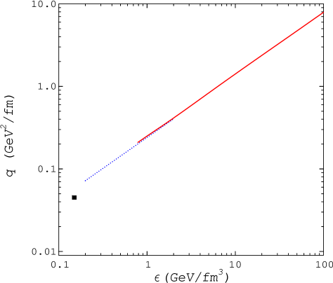
Figure 2.3: Transport coefficient as a function of energy density for different media: cold (marker), massless hot pion gas (dotted curve) and ideal QGP (solid curve) [50].

2.3.2 Quenching weights

The quenching weight is defined as the probability that a hard parton radiates an energy $\Delta E$ due to scattering in spatially extended QCD matter. In Ref. [51], the weights are calculated on the basis of the BDMPS formalism, keeping into account (a) the finite in-medium path length $L$ and (b) the dynamic expansion of the medium. The input parameters for the calculation of the quenching weights are only $L$, the transport coefficient $\hat{q}$ and the parton species (light quark or gluon).

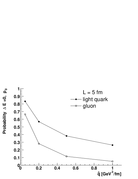
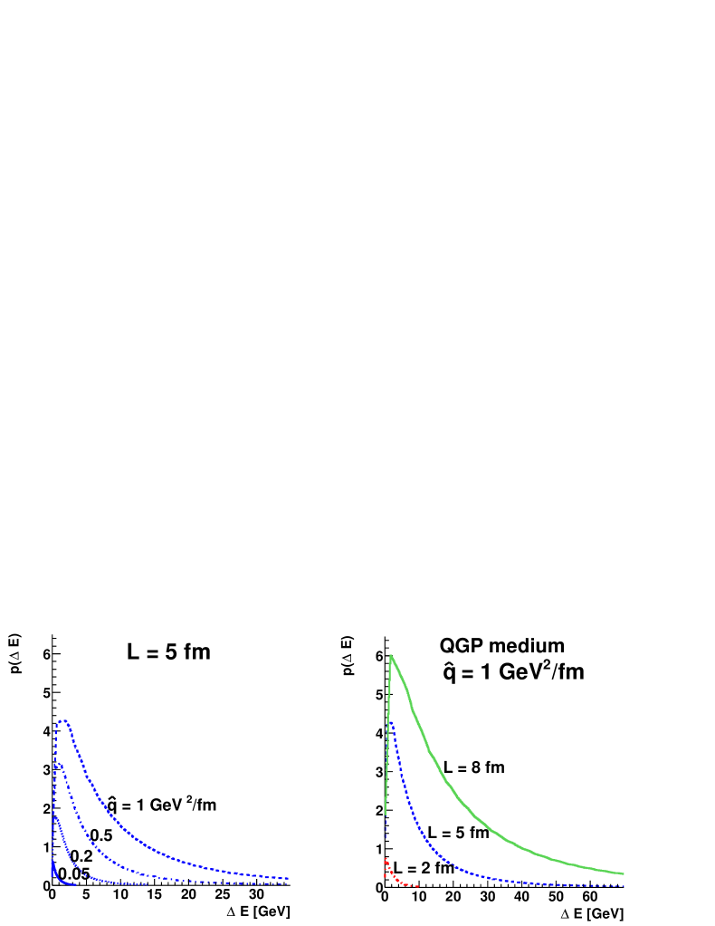
Figure 2.4: The discrete part of the quenching weight (see text) for $L=5\leavevmode\nobreak\ \mathrm{fm}$ as a function of the transport coefficient.

Figure 2.5: Distribution of the continuous part of the quenching weight (see text) for light quarks in different conditions.

The probability distribution $P(\Delta E)$ is obtained as the sum of a discrete and a continuous part,

$$P(\Delta E)=p_{0}\,\delta(\Delta E)+p(\Delta E).$$ (2.10)

The discrete weight $p_{0}$ is interpreted as the probability that no gluon is radiated and hence no in-medium energy loss occurs. The continuous weight is the probability to have an energy loss equal to $\Delta E$, if at least one gluon is radiated.

Using a numerical routine provided by the authors [51] for $\alpha_{s}=1/3$, we have plotted the quenching weights as a function of the different parameters.

Figure 2.5 reports the discrete part $p_{0}$ of the weight as a function of $\hat{q}$ for $L=5\leavevmode\nobreak\ \mathrm{fm}$. The probability that energy loss does not occur is significantly larger for quarks than for gluons, due to their lower QCD coupling, and it decreases as the density of the medium increases; with $\hat{q}=1\leavevmode\nobreak\ \mathrm{GeV}^{2}/\mathrm{fm}$, the probability to have energy loss, $1-p_{0}$, is 75% for a quark and 95% for a gluon.

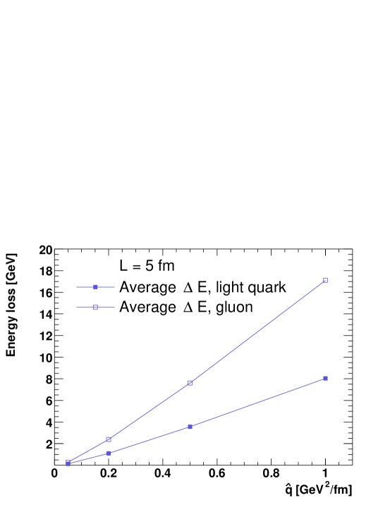
Figure 2.6: Average energy loss for quarks and for gluons, with $L=5\leavevmode\nobreak\ \mathrm{fm}$, as a function of the transport coefficient.

Figure 2.5 reports the distribution of the continuous part $p(\Delta E)$ of the weight for quarks and for different values of $L$ and $\hat{q}$. The average energy loss $\left\langle\Delta E\right\rangle$, calculated taking into account both the discrete and the continuous parts of the quenching weight, for $L=5\leavevmode\nobreak\ \mathrm{fm}$ for quarks and gluons in shown as a function of $\hat{q}$ in Fig. 2.6. As expected (see Eq. (2.6)), $\left\langle\Delta E\right\rangle$ grows approximately linearly with the transport coefficient and, consequently, with the ‘maximum’ gluon energy $\omega_{c}$. For a quark projectile, we find, $\left\langle\Delta E\right\rangle\approx 0.1\times\omega_{c}$.

The average energy loss in a cold medium, $\hat{q}=0.05\leavevmode\nobreak\ \mathrm{GeV}^{2}/\mathrm{fm}$, is predicted to be of order $0.1$-$0.2\leavevmode\nobreak\ \mathrm{MeV}$. In a hot medium with $\hat{q}=1\leavevmode\nobreak\ \mathrm{GeV}^{2}/\mathrm{fm}$, the obtained values are $\left\langle\Delta E\right\rangle\simeq 17\leavevmode\nobreak\ \mathrm{GeV}$ for gluons and $\left\langle\Delta E\right\rangle\simeq 8\leavevmode\nobreak\ \mathrm{GeV}$ for light quarks. Note that the ratio is almost exactly $9/4$.

These spatially integrated energy losses in a hot medium can be ‘translated’ into losses per unit path length, ${\rm d}E/{\rm d}x_{\rm gluons}\approx 3.5\leavevmode\nobreak\ \mathrm{GeV}/\mathrm{fm}$ and ${\rm d}E/{\rm d}x_{\rm quarks}\approx 1.6\leavevmode\nobreak\ \mathrm{GeV}/\mathrm{fm}$. Such values are one order of magnitude larger than those estimated, on the basis of Bjorken’s model, for the collisional energy loss.

Given the $L^{2}$-dependence of the effect, the differential energy loss should be given per unit path length squared: ${\rm d}^{2}E/{\rm d}x^{2}_{\rm gluons}\approx 0.7\leavevmode\nobreak\ \mathrm{GeV}/\mathrm{fm}^{2}$ and ${\rm d}^{2}E/{\rm d}x^{2}_{\rm quarks}\approx 0.3\leavevmode\nobreak\ \mathrm{GeV}/\mathrm{fm}^{2}$.

2.3.3 Dead cone effect for heavy quarks

In Ref. [53] Yu.L. Dokshitzer and D.E. Kharzeev argue that for heavy quarks, because of their large mass, the radiative energy loss should be lower than for light quarks. The predicted consequence of this effect is an enhancement of the ratio of D mesons to pions at moderately large ($5$-$10\leavevmode\nobreak\ \mathrm{GeV}/c$) transverse momenta, with respect to what observed in the absence of energy loss (proton–proton collisions).

Heavy quarks with momenta up to $20$-$30\leavevmode\nobreak\ \mathrm{GeV}/c$ propagate with a velocity which is smaller than the velocity of light, $c$. As a consequence, gluon radiation at angles $\Theta$ smaller than the ratio of their mass to their energy $\Theta_{0}=m_{Q}/E$ is suppressed by destructive quantum interference. In Ref. [54] the soft gluon emission probability off a heavy quark $Q$ in the vacuum is expressed as:

$${\rm d}\sigma_{Q\to Q+g}=\frac{\alpha_{S}\,C_{R}}{\pi}\,\left(1+\frac{\Theta_{0}^{2}}{\Theta^{2}}\right)^{-2}\,{\rm d}\Theta^{2}\,\frac{{\rm d}\omega}{\omega}.$$ (2.11)

The relatively depopulated cone around the $Q$ direction with $\Theta<\Theta_{0}$ is indicated as ‘dead cone’. It is also pointed out that the structure of gluon radiation at large angles, $\Theta\gg\Theta_{0}$ appears to be independent of $m_{Q}/E$ and, thus, identical to that for a light quark jet [54].

A direct consequence of the dead cone effect is the harder fragmentation of heavy quarks, with respect to light quarks and gluons, i.e. the fact that the ‘leading’ (most energetic) hadron produced by a c or b quark carries a larger fraction of the initial quark energy than the leading hadron produced by a massless parton. In the former case, since less gluons are radiated, a larger part of the initial quark energy is available for the leading hadron. In Chapter 8 we shall further discuss the different fragmentation of heavy and light partons.

In Ref. [53] the dead cone effect is assumed to characterize also in-medium gluon radiation and the energy distribution of the radiated gluons (2.5) is estimated to be suppressed by the factor:

$$\left(1+\frac{\Theta_{0}^{2}}{\Theta^{2}}\right)^{-2}=\left[1+\left(\frac{m_{Q}}{E}\right)^{2}\sqrt{\frac{\omega^{3}}{\hat{q}}}\right]^{-2}\equiv F_{\rm H/L}(m_{Q},E,\hat{q},\omega),$$ (2.12)

where the expression for the characteristic gluon emission angle [53] $\Theta\simeq(\hat{q}/\omega^{3})^{1/4}$ has been used. The energy distributions radiated off light quark projectiles and heavy quark projectiles are related as:

$$\left(\omega\frac{{\rm d}I}{{\rm d}\omega}\right)_{\rm Heavy}=F_{\rm H/L}(m_{Q},E,\hat{q},\omega)\times\left(\omega\frac{{\rm d}I}{{\rm d}\omega}\right)_{\rm Light}.$$ (2.13)

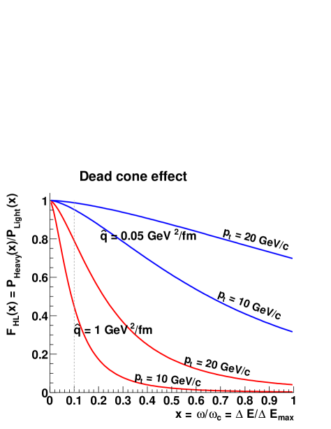
Figure 2.7: Suppression factor for a charm quark as a function of $x=\omega/\omega_{c}$ (see text). The in-medium path length considered is $L=5\leavevmode\nobreak\ \mathrm{fm}$.

The heavy-to-light suppression factor $F_{\rm H/L}$ increases (less suppression) as the heavy quark energy increases (the mass becomes negligible). In Fig. 2.7 we plot the suppression factor for charm quarks ($m_{\rm c}=1.2\leavevmode\nobreak\ \mathrm{GeV}$) as a function of $x=\omega/\omega_{c}\simeq\Delta E/\Delta E_{\rm max}$. This relative scale allows to compare directly situations with different transport coefficients, i.e. different medium densities. For given $\hat{q}$ and $p_{\rm t}$ of the c quark (we then use $E=\sqrt{p_{\rm t}^{2}+m_{\rm c}^{2}}$ assuming production at mid-rapidity), the factor $F_{\rm H/L}(x)$ can be interpreted as the decrease of the probability for emitting a gluon with energy $x\,\omega_{c}$. $F_{\rm H/L}$ decreases at large $x$, indicating that the high-energy part of the gluon radiation spectrum is drastically suppressed by the dead cone effect. In a hot medium, $\hat{q}=1\leavevmode\nobreak\ \mathrm{GeV}^{2}/\mathrm{fm}$, the probability to radiate a gluon with energy $0.1\times\omega_{c}$ (vertical dashed line), which corresponds to the average energy loss (see previous section), is reduced by a factor 0.5 for a $10\leavevmode\nobreak\ \mathrm{GeV}/c$ charm quark and by a factor 0.8 for a $20\leavevmode\nobreak\ \mathrm{GeV}/c$ charm quark, with respect to a light quark.

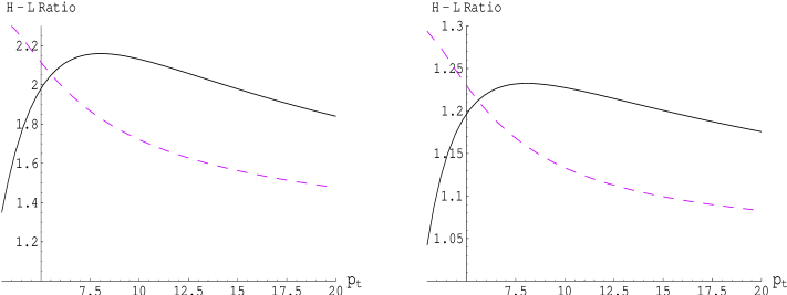
Figure 2.8: Ratio of the quenching factors for charm (H) and light (L) quarks in hot matter with $\hat{q}=1\leavevmode\nobreak\ \mathrm{GeV}^{2}/\mathrm{fm}$ ($L=5\leavevmode\nobreak\ \mathrm{fm}$, left, and $L=2\leavevmode\nobreak\ \mathrm{fm}$, right), as a function of $p_{\rm t}\leavevmode\nobreak\ [\mathrm{GeV}/c]$. Solid lines correspond to unrestricted gluon radiation, while dashed lines are based on the calculation with a cut on the gluon energy $\omega>0.5\leavevmode\nobreak\ \mathrm{GeV}$ [53].

The energy loss probabilities for heavy quarks are not calculated in Ref. [53], as a realistic treatment of nuclear geometry and of the time evolution of QCD matter in the final state was not included. What is provided is a semi-quantitative illustration of the expected consequences of the dead cone effect on the transverse momentum dependence of the ratio of hadrons originating from the fragmentation of heavy and light quarks in heavy ion collisions; because of the lower loss of heavy quarks, such ratio should be enhanced with respect to what measured in pp collisions.

The ${\rm D}/\pi$ ratio is considered, assuming all pions to originate from light quarks. Figure 2.8 shows this ratio for $\hat{q}=1\leavevmode\nobreak\ \mathrm{GeV}^{2}/\mathrm{fm}$, $L=5\leavevmode\nobreak\ \mathrm{fm}$ (left) and $L=2\leavevmode\nobreak\ \mathrm{fm}$ (right), with (dashed) and without (solid) a cut on the minimum energy of the emitted gluons. For $L=5\leavevmode\nobreak\ \mathrm{fm}$, left panel, a factor $\sim 2$ enhancement is expected at $p_{\rm t}\sim 5$-$10\leavevmode\nobreak\ \mathrm{GeV}/c$. The enhancement in the case of a cold medium with $\hat{q}=0.05\leavevmode\nobreak\ \mathrm{GeV}^{2}/\mathrm{fm}$ is found to be of only $\sim 15\%$ [53]. The conclusion of Dokshitzer and Kharzeev is that the ${\rm D}/\pi$ ratio appears to be extremely sensitive to the density of colour charges in QCD matter. Also the B-meson/D-meson ratio is regarded as specially interesting, because the different masses of c and b quarks imply a lower energy loss for the latter.

Concerning the proposed ${\rm D}/\pi$ observable, an important comment has to be made. The proton PDF plot in Fig. 1.12 indicates that, already at RHIC energies, and even more at LHC energies, hadron production come mostly from the fragmentation of gluons rather than light quarks (at the LHC, mostly means $\simeq 80\%$, as we shall show in Chapter 8), and gluons lose more energy than light quarks. On the other hand, D mesons are expected to come essentially from the fragmentation of c quarks. If the c quark comes from a gluon splitting, the gluon must have a virtuality $Q>2\,m_{\rm c}$, meaning that the splitting happens on a spatial scale of $\sim 1/(2\,m_{\rm c})\simeq 0.1\leavevmode\nobreak\ \mathrm{fm}$, so that, also in this case, the c quark sees the whole medium thickness.

Therefore, the ${\rm D}/\pi$ (or, more generally, D/hadrons) ratio is expected to be enhanced both by the different partonic origin of D mesons and non-heavy-flavour hadrons and by the dead cone effect.

2.4 Pre-LHC measurements of open charm production in pA and AA

Charm production in pion–nucleus and proton–nucleus collisions was measured by several experiments in a broad energy range and both the energy dependence and the A dependence are well understood and in agreement with the binary scaling $\sigma^{\scriptstyle{\rm c\overline{c}}}_{\rm pA}={\rm A}\times\sigma^{\scriptstyle{\rm c\overline{c}}}_{\rm pp}$, if no centrality selection is applied. Figure 2.9 presents a recent compilation of charm cross section measurements at different energies: the values refer to forward production ($x_{F}\equiv x_{1}-x_{2}>0$) and, for each pA or $\pi$A system, the cross section was divided by A to obtain the corresponding $\sigma^{\scriptstyle{\rm c\overline{c}}}_{\rm pp}$ [55, 56]. The energy dependence is well reproduced by the PYTHIA model [57] (dotted line).

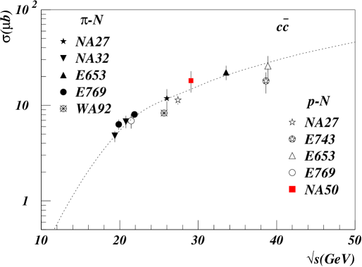
Figure 2.9: Compilation of charm hadroproduction cross section measurements [55, 56]. The figure is explained in the text.

On the other hand, the experimental picture on charm production in ultra-relativistic nucleus–nucleus reactions is quite unclear: there are indications of a possible enhanced production in central Pb–Pb collisions at SPS energy from the dimuon spectra measured by the NA50 experiment [56], while no enhancement is observed in the first measurement of D meson production in Au–Au collisions at RHIC energy by the PHENIX experiment [58], which uses the semi-electronic decay channel. We briefly describe these measurements in the next paragraphs.

The NA38 and NA50 experiments have studied muon pair production in pA, S–U and Pb–Pb collisions at the SPS. The decay of D mesons in the semi-muonic channel allows to indirectly measure the production of $\rm D\overline{D}$ meson pairs by an analysis of the dimuon invariant mass region between the $\phi$ and the J$/\psi$, the so-called intermediate mass region ($1<M_{\mu^{+}\mu^{-}}<3\leavevmode\nobreak\ \mathrm{GeV}$). The reference process used as a normalization is the Drell-Yan (DY), which is supposed to be insensitive to the nature of the medium produced in the collision and which, therefore, scales with the number of binary collisions.

In Ref. [56] it is shown that pA data in the intermediate mass region can be described as a superposition of DY and $\rm D\overline{D}$ dimuons, using PYTHIA to calculate the expected differential spectra of the two contributions. When going to nucleus–nucleus collisions, a linear extrapolation of the pA sources, assuming binary scaling, underestimates the data by an average factor $\sim 1.27$ for S–U and $\sim 1.65$ for Pb–Pb collisions. The expected value of the ratio $({\rm D\overline{D}/DY})$ is calculated using PYTHIA and compared to the value obtained from a fit to the data. The ratio of the fitted to the expected value is reported in Fig. 2.11 as a function of the number of participants, $N_{\rm part}$: in order to describe the data with a simple superimposition of DY plus $\rm D\overline{D}$, the expected charm yield has to be scaled up by a factor that increases roughly linearly with $N_{\rm part}$, reaching $\sim 3.5$ for central Pb–Pb reactions. This result is a bit puzzling, as it is very unlikely that additional charm quarks can be thermally produced at the SPS energy. We remind once more that this is an indirect measurement of charm production.

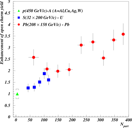
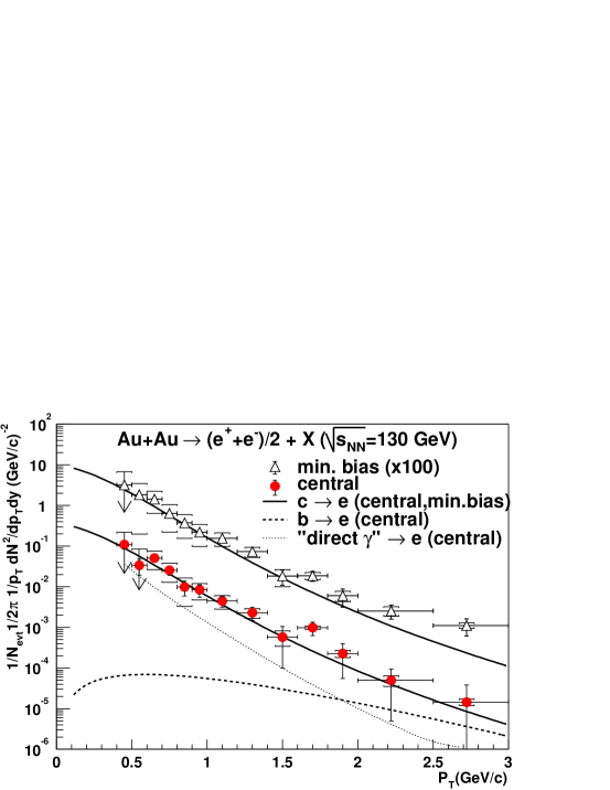
Figure 2.10: The enhancement $E$ of the charm yield needed to describe the dimuon spectrum in the intermediate mass region measured by the NA50 experiment [56].

Figure 2.11: Background-subtracted electron spectra for minimum bias and central collisions, measured by the PHENIX experiment, compared to the expected contributions from D decays (PYTHIA). Also shown, for central collisions only, are the expected contribution from beauty decays (dashed line) and the conversion electron spectrum from a direct photon prediction (dotted line) [58].

The PHENIX experiment at RHIC obtained an indirect estimate of charm production in Au–Au collisions at $\sqrt{s_{\scriptscriptstyle{{\rm NN}}}}=130$ and $200\leavevmode\nobreak\ \mathrm{GeV}$ from the measurement of single electrons at central rapidity ($|\eta|<0.35$). The expected sources of electrons are (1) Dalitz and dielectron decays of light hadrons, (2) photon conversions, (3) kaon semi-electronic decays and (4) semi-electronic decays of D mesons (other contributions, such has beauty decays, are negligible at these energies). The contributions (1)-(3) were estimated using a simulation tuned to reproduce the $\pi^{\pm}$ and $\pi^{0}$ measurements by PHENIX and subtracted. The background-subtracted electron transverse momentum spectra were compared to the expected spectra from charm decays using PYTHIA (the event generator was tuned in order to describe the charm production data at CERN-SPS and at Fermilab and the extrapolation from pp to Au–Au was done with a scaling according to the number of binary collisions). The result at $\sqrt{s_{\scriptscriptstyle{{\rm NN}}}}=130\leavevmode\nobreak\ \mathrm{GeV}$ is shown in Fig. 2.11 [58]. The calculated electron spectra show reasonable agreement, within the relatively large errors, with the data both for the minimum-bias sample and for the central one. A similar agreement is shown also by the data at $\sqrt{s_{\scriptscriptstyle{{\rm NN}}}}=200\leavevmode\nobreak\ \mathrm{GeV}$, where the contribution of photon conversions was directly estimated in a special run with an additional ‘converter layer’ of well defined geometry and material thickness [59].

As we have seen in Section 1.3, PHENIX reports for high-$p_{\rm t}$ hadrons in central Au–Au collisions a substantial suppression relative to binary scaling. Such effect seems not to be present (errors are still large) in the single electrons from charm. This may be explained by lower charm quark in-medium energy loss due to the dead cone effect, described in Section 2.3.3.

In the near future, the NA60 experiment will probably clarify the issue of charm production in nucleus–nucleus collisions at SPS energy and more precise measurements, including also the comparison with pp and pA collisions, will be performed in the energy domain $\sqrt{s_{\scriptscriptstyle{{\rm NN}}}}\sim 100$-$200\leavevmode\nobreak\ \mathrm{GeV}$ by PHENIX.

2.5 Probing the QGP with charm at the LHC

2.5.1 Strategy for the exclusive reconstruction of $\mathrm{D^{0}}$ mesons with ALICE

The investigation of medium-induced effects for charm quarks in the QGP requires a good sensitivity on the momentum distribution of the quarks. Clearly, a direct measurement of the momentum of D mesons would be more effective to this purpose than the indirect measurement via single electrons from the decay ${\rm D}\to e+X$. The exclusive reconstruction of hadronic decays of D mesons is the only way to directly obtain their $p_{\rm t}$ distribution.

The mesons $\mathrm{D^{0}}$ and ${\rm D^{+}}$ (and antiparticles) decay through weak processes and have decay lengths of the order of few tenths of a millimeter, namely $c\tau=(123.7\pm 0.8)\ \mathrm{\mu m}$ for the $\mathrm{D^{0}}$ and $c\tau=(315.3\pm 3.9)\ \mathrm{\mu m}$ for the ${\rm D^{+}}$ [60]. Therefore, the distance between the interaction point (primary vertex) and their decay point (secondary vertex) is measurable.

The selection of a suitable decay channel, which involves only charged-particle products, allows the direct identification of the charm states by computing the invariant mass of fully-reconstructed topologies originating from secondary vertices.

We consider as a benchmark the process ${\rm D^{0}\to K^{-}\pi^{+}}$ (and ${\rm\overline{D^{0}}\to K^{+}\pi^{-}}$); the fraction of $\mathrm{D^{0}}$ mesons which decay in this channel (branching ratio, $BR$) is $(3.80\pm 0.09)\%$ [60].

A sketch of the decay is shown in Fig. 2.12 (the charged tracks are drawn bent by a magnetic field). The main feature of this topology is the presence of two tracks displaced from the primary vertex. The variable that allows to evaluate the displacement of a track is the impact parameter, defined as the distance of closest approach of the track to the primary vertex. Here, we assume the presence of the ALICE solenoidal magnetic field and we indicate as $d_{0}$ the projection of the impact parameter on the bending plane, normal to the field direction. In Chapter 5 a more rigorous definition of the track impact parameter shall be given.

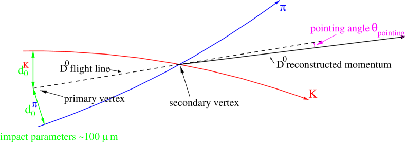
Figure 2.12: Schematic representation of the ${\rm D^{0}\to K^{-}\pi^{+}}$ decay with the impact parameters ($d_{0}$) and the pointing angle ($\theta_{\rm pointing}$).

In Appendix A we show that, in the relativistic limit, the impact parameters of the decay products of a particle with mean proper decay length $c\tau$ have mean value of order $c\tau$. Therefore, the decay products of a $\mathrm{D^{0}}$ particle have typical impact parameters of order $100\leavevmode\nobreak\ \mathrm{\mu m}$.

In this thesis, we study the feasibility for the exclusive reconstruction of $\mathrm{D^{0}}$ decays in heavy ion (and pp) collisions at the LHC by means of the invariant mass analysis of $\mbox{$\mathrm{K}$}^{\mp}\pi^{\pm}$ pairs. Since the background to this decay is combinatorial, the task is a real challenge in the scenario of a central Pb–Pb collision, where, as we have seen in Section 1.4.1, up to $3000$-$4000$ charged tracks are expected to be produced per unit of rapidity.

In order to extract the signal out of this large background the candidate decay tracks are required to satisfy the following ‘secondary vertex criteria’:

1. they are well separated from the interaction vertex, i.e. their impact parameters are of order $100$-$500\leavevmode\nobreak\ \mathrm{\mu m}$; this is mandatory to reject the huge amount of primary tracks produced in a heavy ion collision;

2. the sum of their momenta, which estimates the momentum of the $\mathrm{D^{0}}$ particle, points along the reconstructed $\mathrm{D^{0}}$ flight line; this is realized by requiring the angle $\theta_{\rm pointing}$ between the sum of the momenta and the primary–secondary vertex direction to be small (see sketch in Fig. 2.12).

This strategy demands:

• precise measurement of the momenta to have a good resolution on the invariant mass and, thus, reduce the background in the $\mathrm{D^{0}}$ mass region (in Appendix A we show that, in the relativistic approximation, the invariant mass resolution is proportional to the momentum resolution);

• measurement of the impact parameters with resolution of the order of $50\leavevmode\nobreak\ \mathrm{\mu m}$ for the decay products of the $\mathrm{D^{0}}$;

• particle identification to tag the two decay products and reject $\pi^{\mp}\pi^{\pm}$ pairs, which are a large part of the combinatorial background.

The ALICE central barrel, described in Chapter 4, was designed to fulfill these requirements. It, in fact, provides tracking and precise impact parameter measurement, with a Time Projection Chamber and a silicon Inner Tracking System, and $\mbox{$\mathrm{K}$}/\pi$ separation, with a Time-of-Flight detector, over the pseudorapidity range $-0.9<\eta<0.9$. The results on the feasibility of the strategy here outlined are reported in Chapter 6.

2.5.2 Outline for the physics sensitivity studies

As discussed in Section 2.2, the two final state effects that can be investigated by means of fully-reconstructed $\mathrm{D^{0}}$ mesons in Pb–Pb collisions at the LHC are the c quark energy loss and the possible additional production of $\mathrm{c\overline{c}}$ pairs in the hot medium.

The sensitivity to thermal charm production goes beyond the scope of this work and it is an interesting issue for the charm studies in the near future.

Energy loss, or quenching, effects can be addressed with two independent approaches, which we have already introduced when presenting the recent interesting observations at RHIC (see Section 1.3):

Leading particle analysis:

study of the medium-induced modification of the transverse momentum distribution of identified D mesons.

Correlations analysis:

study of the event structure, in terms of angular correlations of the produced particles with an identified D meson in the event.

In this work we concentrate on the leading particle analysis, as it is more suitable for comparison of the results with model predictions and to disentangle different effects, by looking for example at the ${\rm D}/hadrons$ ratio to quantify the dead cone suppression of medium-induced radiation. However, also the study of the structure of charm-tagged jets by means of reconstructed ${\rm D^{0}\to K^{-}\pi^{+}}$ decays is of great interest and is currently being investigated.

We consider the nuclear modification factor, $R_{\rm AA}$, defined as the ratio of the $p_{\rm t}$ distribution measured in central AA collisions, divided by the number of estimated binary nucleon–nucleon (NN) collisions, to the $p_{\rm t}$ distribution measured in pp collisions, scaled to the same c.m.s. energy:

$$R_{\rm AA}(p_{\rm t})=\frac{{\rm d}\sigma^{\rm AA}/{\rm d}p_{\rm t}/{\rm binary\leavevmode\nobreak\ NN\leavevmode\nobreak\ collision}}{{\rm d}\sigma^{\rm pp}/{\rm d}p_{\rm t}}=\frac{{\rm d}N^{\rm AA}/{\rm d}p_{\rm t}}{N_{\rm coll}\times{\rm d}N^{\rm pp}/{\rm d}p_{\rm t}}$$ (2.14)

The choice of this ratio allows to reduce the systematic uncertainties, as the errors which are common to AA and pp data cancel out.

If no nuclear effects were present the nuclear modification factor would be 1. Initial state effects (shadowing and intrinsic $k_{\rm t}$ broadening) and possible thermal charm production should affect $R_{\rm AA}$ only for relatively low transverse momenta ($p_{\rm t}<5$-$7\leavevmode\nobreak\ \mathrm{GeV}/c$), as discussed in Section 2.2. Above this region energy loss can be reasonably expected to be the only relevant effect. The behaviour of $R_{\rm AA}$ in presence of an energy loss of average magnitude $\Delta E$ (for the hadrons) can be qualitatively described assuming the $p_{\rm t}$ distribution to follow a power law d$N^{\rm pp}/$d$p_{\rm t}\propto p_{\rm t}^{-n}$. In this case, in fact, we have ${\rm d}N^{\rm AA}/{\rm d}p_{\rm t}/N_{\rm coll}\propto(p_{\rm t}+\Delta E)^{-n}$ and, consequently:

$$R_{\rm AA}(p_{\rm t})\simeq\left(1+\frac{\Delta E}{p_{\rm t}}\right)^{-n}.$$ (2.15)

This ratio is clearly lower than 1 and, if $\Delta E$ does not depend on $p_{\rm t}$, as it is the case for radiative energy loss in the BDMPS formulation, Eq. (2.6), $R_{\rm AA}$ is expected to increase with $p_{\rm t}$ and reach 1 for $p_{\rm t}\gg n\,\Delta E$.  

The sensitivity study (presented in Chapter 8, except where differently indicated) will be outlined as follows:

• estimate of the accessible $p_{\rm t}$ range and of the main experimental uncertainties on the $p_{\rm t}$ distribution of $\mathrm{D^{0}}$ mesons, in pp and in Pb–Pb (Chapters 6 and 7);

• study of a strategy for the extrapolation to $5.5\leavevmode\nobreak\ \mathrm{TeV}$ of the $p_{\rm t}$ distribution measured in pp at $14\leavevmode\nobreak\ \mathrm{TeV}$ (Chapter 7);

• study of the effect of energy loss on the $p_{\rm t}$ distributions of c quarks and D mesons; the quenching weights calculated by Salgado and Wiedemann [51] will be used, with a correction that takes into account the dead cone;

• estimate of the experimental uncertainties on the nuclear modification factor for $\mathrm{D^{0}}$ mesons;

• experimental sensitivity with respect to the predictions of the quenching model, without and with dead cone effect;

• estimate of the experimental uncertainty on the ${\rm D}/charged\leavevmode\nobreak\ hadrons$ (D/$h$) ratio, defined as

  $$R_{{\rm D}/h}(p_{\rm t})=R_{\rm AA}^{\rm D}(p_{\rm t})/R_{\rm AA}^{h}(p_{\rm t}),$$ (2.16)

  and experimental sensitivity for this ratio, without and with dead cone; we point out that, being in practice a double ratio Pb–Pb/Pb–Pb$\times{\rm pp/pp}$, $R_{{\rm D}/h}$ is a very sensitive variable since most systematic errors cancel out.

The main goal of this analysis is to assess the capability of ALICE to study and compare the effects induced by the medium on energetic gluons and heavy quarks, which are predicted to be different on the basis of well-established properties of quantum chromodynamics, like the colour charges of quarks and gluons and the suppression of small-angle radiation off massive quarks. The capability to experimentally investigate such expected differences allows to test the coherence of our understanding of the properties of the matter produced in high-energy nucleus–nucleus collisions.

Chapter 3 Charm and beauty production at the LHC

In the previous chapter we have discussed the physics motivations for the study of charm (or, more generally, heavy flavour) production in nucleus–nucleus collisions at the LHC. In this chapter we define the baseline used in the scope of this thesis for what concerns the charm and beauty production cross sections at the LHC and the kinematical distributions of the produced heavy quarks.

The most recent results of next-to-leading order perturbative QCD calculations for the cross sections in nucleon–nucleon collisions at LHC energies are presented in Section 3.1, where also the theoretical uncertainties are discussed. In Section 3.2 the extrapolations to Pb–Pb and p–Pb collisions are described. Some relevant kinematical distributions for c and b quarks are shown in Section 3.3. The PYTHIA event generator was tuned in order to reproduce the heavy quarks transverse momentum distributions given by the NLO calculations (Section 3.4). Finally, in Section 3.5 we report the yields and the kinematical distributions for charm and beauty mesons.

3.1 Cross sections in nucleon–nucleon collisions

In this section we present the status of the cross section calculations in nucleon–nucleon collisions and their comparison with existing data up to a c.m.s. energy of $\simeq 65\leavevmode\nobreak\ \mathrm{GeV}$. We then report the results for LHC energies. The extrapolation to heavy ion collisions is described in the next section.

Figure 3.1: Total charm production cross section from pp and pA measurements compared to NLO calculations [36] with MRS D-’ (solid), MRST HO (dashed) and MRST LO (dot-dashed) parton distributions.

Figure 3.2: Comparison with b quark production cross section integrated over $p_{\rm t}>p_{\rm t}^{\rm min}$ from (a) UA1 [61] and (b) CDF and D0 [62]. The NLO calculations are with MRS D-’ (solid) and GRV HO (dashed) parton distributions.

The existing data on total charm production cross section in pp and pA collisions up to ISR energies are compared in Fig. 3.2 with NLO calculations by R. Vogt [36]. In Fig. 3.2 a NLO calculation from Ref. [63] is compared to the data in $\mathrm{p\overline{p}}$ collisions from UA1, CDF and D0, for which the b quark production cross section integrated for $p_{\rm t}>p_{\rm t}^{\rm min}$ is given. These measurements are taken in the central rapidity region ($|y|<1.5$ for UA1, $|y|<1$ for CDF and D0). All the calculations have been performed using the following values for the heavy quark masses ($m_{\rm c}$, $m_{\rm b}$) and for the factorization and renormalization scales ($\mu_{F}$, $\mu_{R}$):

$$m_{\rm c}=1.2\leavevmode\nobreak\ \mathrm{GeV}\,\,\,\,\,\,\,\,\,\,\,\,\,\,\,\,\,\,\,\,\,\,\,\,\,\,\,\,\,\,\,\,\,\,\,\,\,\,\,\mu_{F}=\mu_{R}=2\,\mu_{0}$$ (3.1)

for charm, and

$$m_{\rm b}=4.75\leavevmode\nobreak\ \mathrm{GeV}\,\,\,\,\,\,\,\,\,\,\,\,\,\,\,\,\,\,\,\,\,\,\,\,\,\,\,\,\,\,\,\,\,\,\,\,\,\,\,\mu_{F}=\mu_{R}=\mu_{0}$$ (3.2)

for beauty; $\mu_{0}=\sqrt{(p_{\rm t,Q}^{2}+p_{\rm t,\overline{Q}}^{2})/2+m_{Q}^{2}}$ is approximately equal to the transverse mass of the produced heavy quarks.

For both charm and beauty the theory describes the present data reasonably well.

Table 3.1: NLO calculation [64] for the total $\mathrm{c\overline{c}}$  and $\mathrm{b\overline{b}}$  cross sections in pp collisions at 5.5, 8.8 and 14 $\mathrm{TeV}$, using the MRST HO and CTEQ 5M1 parton distribution functions.

		$\sigma_{{\rm pp}}^{\scriptstyle{\rm c\overline{c}}}[{\rm mb}]$			$\sigma_{{\rm pp}}^{\scriptstyle{\rm b\overline{b}}}[{\rm mb}]$
$\sqrt{s}$	$5.5\leavevmode\nobreak\ \mathrm{TeV}$	$8.8\leavevmode\nobreak\ \mathrm{TeV}$	$14\leavevmode\nobreak\ \mathrm{TeV}$	$5.5\leavevmode\nobreak\ \mathrm{TeV}$	$8.8\leavevmode\nobreak\ \mathrm{TeV}$	$14\leavevmode\nobreak\ \mathrm{TeV}$
MRST HO	5.9	8.4	10.3	0.19	0.28	0.46
CTEQ 5M1	7.4	9.6	12.1	0.22	0.31	0.55
Average	6.6	9.0	11.2	0.21	0.30	0.51

The results for LHC energies ($\sqrt{s}=$ 5.5, 8.8 and 14 $\mathrm{TeV}$) are reported in Table 3.1. These values are obtained using the NLO pQCD calculation implemented in the program by M. Mangano, P. Nason and G. Ridolfi [64] (HVQMNR) and two sets of parton distribution functions, MRST HO [28] and CTEQ 5M1 [29], which include the small-$x$ HERA results. The difference due to the choice of the parton distribution functions is relatively small ($\sim 20$-$25\%$ at 5.5 $\mathrm{TeV}$, slightly lower at 14 $\mathrm{TeV}$). We chose to use as a baseline the average, also reported in the table, of the values obtained with these two sets of PDF.

Table 3.2: Charm and beauty total cross sections at NLO with different choices of the parameters $m_{\rm c}$ ($m_{\rm b}$), $\mu_{F}$ and $\mu_{R}$ [65]. In the last column the ratio of the cross sections at 5.5 TeV and at 14 TeV is reported.

	parameters	5.5 $\mathrm{TeV}$	14 $\mathrm{TeV}$	ratio 5.5 TeV/14 TeV
	$m_{\rm c}=1.5\leavevmode\nobreak\ \mathrm{GeV}$
	$\mu_{R}=2\mu_{0}\,\,\,\,\,\,\mu_{F}=2\mu_{0}$	3.7	7.3	0.51
	$m_{\rm c}=1.2$ GeV
	$\mu_{R}=\mu_{0}\,\,\,\,\,\,\mu_{F}=2\mu_{0}$	9.2	16.7	0.55
	$m_{\rm c}=1.5$ GeV
	$\mu_{R}=\mu_{0}\,\,\,\,\,\,\mu_{F}=2\mu_{0}$	5.4	10.4	0.52
	$m_{\rm c}=1.8\leavevmode\nobreak\ \mathrm{GeV}$
$\sigma_{{\rm pp}}^{\scriptstyle{\rm c\overline{c}}}[{\rm mb}]$	$\mu_{R}=\mu_{0}\,\,\,\,\,\,\mu_{F}=2\mu_{0}$	3.4	6.8	0.50
	$m_{\rm b}=4.5\leavevmode\nobreak\ \mathrm{GeV}$
	$\mu_{R}=\mu_{0}\,\,\,\,\,\,\mu_{F}=\mu_{0}$	0.20	0.51	0.39
	$m_{\rm b}=4.75\leavevmode\nobreak\ \mathrm{GeV}$
	$\mu_{R}=\mu_{0}\,\,\,\,\,\,\mu_{F}=\mu_{0}$	0.17	0.43	0.40
	$m_{\rm b}=5\leavevmode\nobreak\ \mathrm{GeV}$
	$\mu_{R}=\mu_{0}\,\,\,\,\,\,\mu_{F}=\mu_{0}$	0.15	0.37	0.41
	$m_{\rm b}=4.75\leavevmode\nobreak\ \mathrm{GeV}$
	$\mu_{R}=0.5\mu_{0}\,\,\,\,\,\,\mu_{F}=2\mu_{0}$	0.26	0.66	0.39
	$m_{\rm b}=4.75\leavevmode\nobreak\ \mathrm{GeV}$
$\sigma_{{\rm pp}}^{\mbox{$\scriptstyle\mathrm{b\overline{b}}$}}[{\rm mb}]$	$\mu_{R}=2\mu_{0}\,\,\,\,\,\,\mu_{F}=0.5\mu_{0}$	0.088	0.20	0.44

The dependence on the PDF set represents only a part of the error on the theoretical estimate. An evaluation of the theoretical uncertainties was done by M. Mangano by varying the $m_{\rm c}$ ($m_{\rm b}$), $\mu_{F}$ and $\mu_{R}$ parameters and is reported in Table 3.2 [65]. This table shows that, at LHC energies, the theoretical uncertainties span a factor $\sim 2$-$3$ in the total production cross section of both charm and beauty quarks. In the last column of the table we report the ratio of the cross section at 5.5 TeV to that at 14 TeV. Despite the large spread of the absolute values, the ratio is much less dependent on the choice of the parameters; its value is $\simeq 0.52$ for charm and $\simeq 0.41$ for beauty. This indicates that pQCD can be used to compare the cross sections measured in Pb–Pb collisions at $\sqrt{s_{\scriptscriptstyle{{\rm NN}}}}=5.5\leavevmode\nobreak\ \mathrm{TeV}$ to those measured in p–Pb at $\sqrt{s_{\scriptscriptstyle{{\rm NN}}}}=8.8\leavevmode\nobreak\ \mathrm{TeV}$ and in pp at $\sqrt{s}=14\leavevmode\nobreak\ \mathrm{TeV}$. The uncertainty introduced by the energy extrapolation is estimated in Chapter 7.

Yields in proton–proton collisions at $\sqrt{s}=14\leavevmode\nobreak\ \mathrm{TeV}$

Using a proton–proton inelastic cross section $\sigma^{\rm inel}_{{\rm pp}}=70\leavevmode\nobreak\ {\rm mb}$ at 14 $\mathrm{TeV}$ [24] and the average heavy flavour cross sections in the last row of Table 3.1, we calculate the yields for the production of $Q\overline{Q}$ pairs as:

$$N_{{\rm pp}}^{\scriptstyle Q\overline{Q}}=\sigma_{{\rm pp}}^{\scriptstyle Q\overline{Q}}\bigg{/}\sigma^{\rm inel}_{{\rm pp}}.$$ (3.3)

We obtain 0.16 $\mathrm{c\overline{c}}$ pairs and 0.0072 $\mathrm{b\overline{b}}$ pairs per event.

3.2 Extrapolation to heavy ion collisions

In this section we derive the extrapolation of the cross sections and yields to central Pb–Pb collisions first, and then to p–Pb collisions. We also point out the different weight of the nuclear shadowing effect in the two cases, for charm and beauty production.

3.2.1 Nucleus–nucleus collisions

If no nuclear effects are taken into account, a nucleus–nucleus collision can be considered as a superposition of independent nucleon–nucleon collisions. Thus, the cross section for hard processes in heavy ion collisions can be calculated using a simple geometrical extrapolation from pp collisions, i.e. assuming that the hard cross section scales from pp to nucleus–nucleus collisions proportionally to the number of inelastic nucleon–nucleon collisions.

Nuclear effects —such as nuclear shadowing, broadening of the parton intrinsic transverse momentum ($k_{\rm t}$), energy loss, as well as possible enhancements due to thermal production in the medium— can modify this geometrical scaling from pp to nucleus–nucleus collisions. Such effects are, indeed, what we want to measure. We chose to include in the simulation only the nuclear shadowing and the broadening of the intrinsic $k_{\rm t}$, since they are well established effects. The first effect modifies the total hard cross section, while the broadening of the intrinsic $k_{\rm t}$ affects only the kinematic distributions of the produced heavy quarks. Nuclear shadowing can be accounted for by recalculating the hard cross section in elementary nucleon–nucleon collisions with modified parton distribution functions, as we have seen in Section 1.5.1, and extrapolating to the nucleus–nucleus case.

The extrapolation, based on the Glauber model [66, 67], is derived for the collision of two generic nuclei with mass numbers A and B, and numerical examples are given for the specific case of Pb–Pb reactions at $\sqrt{s_{\scriptscriptstyle{{\rm NN}}}}=5.5\leavevmode\nobreak\ \mathrm{TeV}$.

We are interested in the cross section for a sample of events in a given centrality range, defined by the trigger settings. The centrality selection can be assumed to correspond to a cut on the impact parameter $b$ of the collision: $0\leq b<b_{c}$. The sample of events defined by this cut contains a fraction of the total number of inelastic collisions, i.e. of the total inelastic cross section, given by

$$F(b_{c})=\int_{0}^{b_{c}}{\rm d}b\,\frac{{\rm d}\sigma^{\rm inel}_{\rm AB}}{{\rm d}b}\bigg{/}\int_{0}^{\infty}{\rm d}b\,\frac{{\rm d}\sigma^{\rm inel}_{\rm AB}}{{\rm d}b}.$$ (3.4)

The definition of the centrality in terms of fraction of the inelastic cross section is more appropriate, since the cross section is directly measured, while the impact parameter estimation depends on the model used to describe the geometry of the collision.

In the following, we consider the most central class of events that can be selected by means of the ALICE Zero Degree Calorimeters (briefly described in Chapter 4). This class corresponds to 5% of the total inelastic cross section and to a maximum impact parameter $b_{c}$ of about $3.5\leavevmode\nobreak\ {\rm fm}$.

The inelastic cross section corresponding to a given centrality selection is found integrating the interaction probability up to impact parameter $b_{c}$:

$$\sigma_{{\rm AB}}^{\mathrm{inel}}(b_{c})=\int_{0}^{b_{c}}{\rm d}b\,\frac{{\rm d}\sigma^{\rm inel}_{\rm AB}}{{\rm d}b}=2\pi\int_{0}^{b_{c}}b\,{\rm d}b\,\,\left\{1-[1-\sigma_{\scriptscriptstyle{{\rm NN}}}T_{{\rm AB}}(b)]^{{\rm AB}}\right\}$$ (3.5)

where the value $\sigma_{\scriptscriptstyle{{\rm NN}}}=60\leavevmode\nobreak\ {\rm mb}$ was used as the nucleon–nucleon inelastic cross section at 5.5 TeV [60], and the total thickness function $T_{{\rm AB}}$

$$T_{{\rm AB}}(b)=\int{\rm d}^{2}s\,T_{\rm A}(\vec{s})\,T_{\rm B}(\vec{s}-\vec{b})$$ (3.6)

(vectors defined as in Fig. 3.3, left) is expressed in terms of the thickness function of the nucleus $T_{i}(\vec{s})=\int{\rm d}z\,\rho_{i}(z,\vec{s})$ for $i={\rm A,\,B}$, where $\rho_{i}$ is the Wood-Saxon nuclear density profile [68] —the thickness function is normalized to unity: $\int{\rm d^{2}}s\,T_{i}(\vec{s})=1$. In Fig. 3.3 (right) the inelastic cross section (3.5) is shown as a function of $b_{c}$.

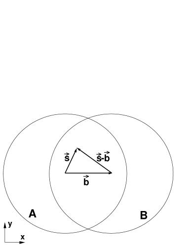
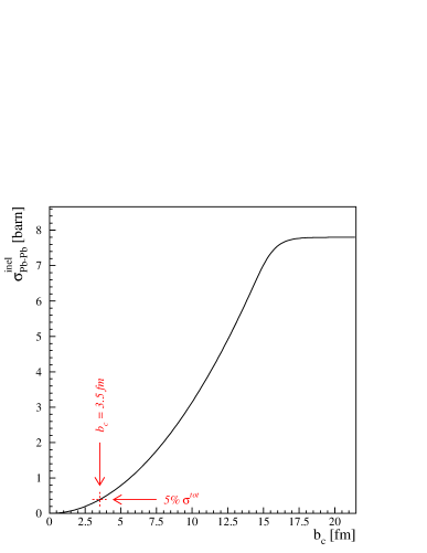
Figure 3.3: Left: collision geometry in the plane transverse to the beam line. Right: inelastic Pb–Pb cross section as a function of the impact parameter cut $b<b_{c}$; the value corresponding to 5% of the total inelastic cross section is indicated.

The average number of inelastic collisions for a given impact parameter $b$ is:

$$\sigma_{\scriptscriptstyle{{\rm NN}}}\cdot{\rm AB}\,\,T_{{\rm AB}}(b).$$ (3.7)

By replacing the inelastic nucleon–nucleon cross section $\sigma_{\scriptscriptstyle{{\rm NN}}}$ with the elementary cross section for a given hard process $\sigma_{\rm pp}^{\rm hard}$, we obtain the average number of inelastic collisions that yield the considered hard process:

$$\sigma_{\rm pp}^{\rm hard}\cdot{\rm AB}\,\,T_{{\rm AB}}(b),$$ (3.8)

and the cross section for hard processes for $0\leq b<b_{c}$:

$$\sigma_{{\rm AB}}^{\mathrm{hard}}(b_{c})=\sigma_{{\rm pp}}^{\mathrm{hard}}\cdot 2\pi\,\int_{0}^{b_{c}}b\,{\rm d}b\,\,{\rm AB}\,\,T_{{\rm AB}}(b).$$ (3.9)

For minimum-bias collisions ($b_{c}=+\infty$), we have:

$$\sigma_{{\rm AB}}^{\mathrm{hard}}=\sigma_{{\rm pp}}^{\mathrm{hard}}\,{\rm AB}.$$ (3.10)

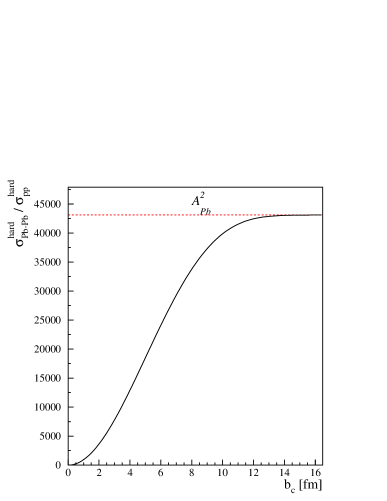
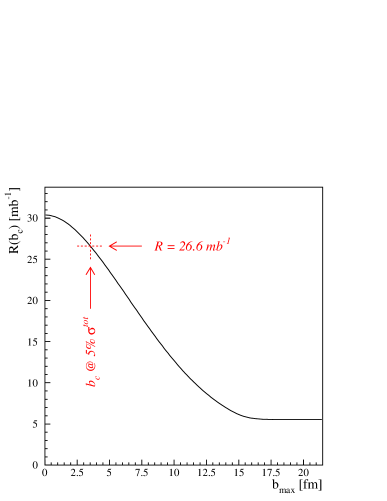
Figure 3.4: Left: cross section for a hard process in Pb–Pb collisions relative to the one in nucleon-nucleon collisions as a function of the impact parameter cut $b<b_{c}$. Right: yield of the hard process in Pb–Pb collisions relative to the cross section in nucleon–nucleon collisions as a function of the impact parameter cut $b<b_{c}$.

The ratio of the hard cross section in nucleus–nucleus collisions, with a centrality cut $b<b_{c}$, relative to the cross section in nucleon–nucleon interactions is (see Fig. 3.4, left):

$$f^{\mathrm{hard}}(b_{c})=\frac{\sigma_{{\rm AB}}^{\mathrm{hard}}(b_{c})}{\sigma_{{\rm pp}}^{\mathrm{hard}}}=2\pi\int_{0}^{b_{c}}b\,{\rm d}b\,\,{\rm AB}\,\,T_{{\rm AB}}(b).$$ (3.11)

The number (yield) of hard processes per triggered event is:

$$N_{{\rm AB}}^{\mathrm{hard}}(b_{c})=\frac{\sigma_{{\rm AB}}^{\mathrm{hard}}(b_{c})}{\sigma_{{\rm AB}}^{\mathrm{inel}}(b_{c})}=R(b_{c})\cdot\sigma_{{\rm pp}}^{\mathrm{hard}}$$ (3.12)

where (Fig. 3.4, right)

$$R(b_{c})=\frac{\int_{0}^{b_{c}}b\,{\rm d}b\,\,{\rm AB}\,\,T_{{\rm AB}}(b)}{\int_{0}^{b_{c}}b\,{\rm d}b\,\,\left\{1-[1-\sigma_{\scriptstyle{{\rm NN}}}T_{{\rm AB}}(b)]^{{\rm AB}}\right\}}.$$ (3.13)

For a 5% centrality cut in Pb–Pb collisions, the yield $N_{\rm AB}^{\rm hard}$ is obtained by multiplying the elementary cross sections by $26.6\leavevmode\nobreak\ {\rm mb}^{-1}$.

Cross sections and yields in Pb–Pb collisions at $\sqrt{s_{\scriptscriptstyle{{\rm NN}}}}=5.5\leavevmode\nobreak\ \mathrm{TeV}$

We used the EKS98 parameterization [33] of nuclear shadowing (introduced in Section 1.5.1) to recalculate the elementary charm and beauty production cross sections. The reduction of the cross section due to shadowing amounts to about 35% for $\mathrm{c\overline{c}}$ pairs, while it amounts only to about 15% for $\mathrm{b\overline{b}}$ pairs, since, as pointed out in Section 1.5.1, beauty production corresponds to larger values of Bjorken $x$ (due to the larger mass of the b quark), that are less affected by the shadowing suppression (Fig. 1.13). In Section 3.3 we will show how nuclear shadowing modifies the heavy quark kinematical distributions.

The values of the parton intrinsic $k_{\rm t}$ used in the simulation were taken from Ref. [36].

Table 3.3 summarizes the charm and beauty total cross sections and yields in pp (with and without shadowing) and Pb–Pb collisions (5% centrality selection) at $\sqrt{s_{\scriptscriptstyle{{\rm NN}}}}=5.5\leavevmode\nobreak\ \mathrm{TeV}$. The values shown correspond to the average of the results obtained with MRST HO and CTEQ 5M1 parton distribution functions.

Table 3.3: Total cross sections and yields for charm and beauty production in pp and Pb–Pb collisions at $\sqrt{s_{\scriptscriptstyle{{\rm NN}}}}=5.5\leavevmode\nobreak\ \mathrm{TeV}$. The effect of shadowing is shown as the ratio $C_{\rm shad}$ of the cross section calculated with and without the modification of the parton distribution functions. For the Pb–Pb case the centrality selection corresponds to 5% of the total inelastic cross section.

		Charm	Beauty
	w/o shadowing	6.64	0.21
$\sigma^{\scriptstyle Q\overline{Q}}_{{\rm pp}}\,[{\rm mb}]$	w/ shadowing	4.32	0.18
$C_{\rm shad}$		0.65	0.84
$\sigma^{\scriptstyle Q\overline{Q}}_{\rm Pb-Pb}[{\rm b}]$	$5\%\leavevmode\nobreak\ \sigma^{\rm tot}$	45.0	1.79
$N^{\scriptstyle Q\overline{Q}}_{\rm Pb-Pb}$	$5\%\leavevmode\nobreak\ \sigma^{\rm tot}$	115	4.56

3.2.2 Proton–nucleus collisions

For the extrapolation to proton–nucleus collisions we use the geometrical Glauber-based method already described for the case of nucleus–nucleus collisions. If we consider minimum-bias collisions (with no centrality selection), and we use $\rm B=1$ and $T_{\rm B}(\vec{s})=\delta(\vec{s})$ for the proton, the total cross section for hard processes (3.9) becomes:

$$\sigma_{{\rm pA}}^{\mathrm{hard}}=\sigma_{{\rm pp}}^{\mathrm{hard}}\cdot 2\pi\,\int_{0}^{\infty}b\,{\rm d}b\,\,{\rm A}\,\,T_{{\rm A}}(b)={\rm A}\,\sigma_{{\rm pp}}^{\mathrm{hard}}.$$ (3.14)

The number of hard processes per minimum-bias pA collision is:

$$N^{\rm hard}_{\rm pA}={\rm A}\,\sigma^{\rm hard}_{\rm pp}\bigg{/}\sigma^{\rm inel}_{\rm pA}.$$ (3.15)

Cross sections and yields in p–Pb collisions at $\sqrt{s_{\scriptscriptstyle{{\rm NN}}}}=8.8\leavevmode\nobreak\ \mathrm{TeV}$

We consider, as the reference proton–nucleus system, p–Pb (and Pb–p). In this case we have $\sqrt{s_{\scriptscriptstyle{{\rm NN}}}}=8.8\leavevmode\nobreak\ \mathrm{TeV}$ and the rapidity shift is $\Delta y=+0.47$ ($-0.47$ for Pb–p).

Using $\rm A=208$ and $\sigma_{\rm p-Pb}^{\rm inel}=1.9$ barn [24], the yield of $Q\overline{Q}$ pairs per minimum-bias collision is:

$$N^{\scriptstyle Q\overline{Q}}_{\rm p-Pb}=\sigma^{\scriptstyle Q\overline{Q}}_{\rm pp}\cdot 0.109\leavevmode\nobreak\ {\rm mb^{-1}}.$$ (3.16)

As for the Pb–Pb case, the effect of nuclear shadowing was accounted for by using the EKS98 parameterization [33]. Clearly, the effect is lower for p–Pb, since one of the colliding nuclei is a proton: the reduction of the cross sections due to nuclear shadowing is 20% for charm and 10% for beauty.

The cross sections and yields for charm and beauty production in pp (with and without shadowing) and minimum-bias p–Pb collisions at $\sqrt{s_{\scriptscriptstyle{{\rm NN}}}}=8.8\leavevmode\nobreak\ \mathrm{TeV}$ are reported in Table 3.4. The values shown correspond to the average of the results obtained with MRST HO and CTEQ 5M1 parton distribution functions.

A summary of the production yields and of the average magnitude of nuclear shadowing in the three considered colliding systems is presented in Table 3.5.

Table 3.4: Total cross sections and yields for charm and beauty production in pp and p–Pb collisions at $\sqrt{s_{\scriptscriptstyle{{\rm NN}}}}=8.8\leavevmode\nobreak\ \mathrm{TeV}$. The effect of shadowing is shown as the ratio $C_{\rm shad}$ of the cross section calculated with and without the modification of the parton distribution functions.

		Charm	Beauty
	w/o shadowing	9.00	0.30
$\sigma^{\scriptstyle Q\overline{Q}}_{{\rm pp}}\,[{\rm mb}]$	w/ shadowing	7.16	0.27
$C_{\rm shad}$		0.80	0.90
$\sigma^{\scriptstyle Q\overline{Q}}_{\rm p-Pb}[{\rm b}]$		1.49	0.056
$N^{\scriptstyle Q\overline{Q}}_{\rm p-Pb}$		0.78	0.029

Table 3.5: Summary table of the production yields and of the average magnitude of nuclear shadowing in pp, p–Pb and Pb–Pb.

		Charm			Beauty
system	pp	p–Pb	Pb–Pb	pp	p–Pb	Pb–Pb
centrality	min.-bias	min.-bias	centr. (5%)	min.-bias	min.-bias	centr. (5%)
$\sqrt{s_{\scriptscriptstyle{{\rm NN}}}}$	$14\leavevmode\nobreak\ \mathrm{TeV}$	$8.8\leavevmode\nobreak\ \mathrm{TeV}$	$5.5\leavevmode\nobreak\ \mathrm{TeV}$	$14\leavevmode\nobreak\ \mathrm{TeV}$	$8.8\leavevmode\nobreak\ \mathrm{TeV}$	$5.5\leavevmode\nobreak\ \mathrm{TeV}$
$N^{\scriptstyle Q\overline{Q}}$/ev	0.16	0.78	115	0.0072	0.029	4.56
$C_{\rm shad}$	1	0.80	0.65	1	0.90	0.84

3.3 Heavy quark kinematical distributions

Figures 3.5 and 3.6 present the transverse momentum and rapidity distributions, obtained using the NLO pQCD program HVQMNR, for c and b quarks, respectively. The distributions for Pb–Pb and p–Pb are normalized to the cross section per nucleon–nucleon collision. Nuclear shadowing is included via the EKS98 parameterization and intrinsic $k_{\rm t}$ broadening is included as well. In the case of p–Pb events the rapidity distribution in the centre-of-mass frame is plotted; the rapidity distribution in the laboratory frame would be shifted by $\Delta y=0.47$.

We notice that the $p_{\rm t}$ distributions for pp collisions at 5.5, 8.8 and 14 TeV (top-left panel) have essentially the same shape.

The comparison of the $p_{\rm t}$ distributions for pp and Pb–Pb (and for pp and p–Pb) at the same centre-of-mass energy shows that, as expected, nuclear shadowing affects heavy quark production only for relatively low transverse momenta ($p_{\rm t}<5$-$6\leavevmode\nobreak\ \mathrm{GeV}/c$ with EKS98), where the $\mathrm{Q\overline{Q}}$ pairs are produced by low-$x$ gluons. This is clearly seen in the ratios of the distributions, reported in the insets.

A relevant feature of $\mathrm{Q\overline{Q}}$ production in p–Pb collisions is a depletion in the forward region (where the proton goes) of the rapidity distributions. This effect is due to the shadowing which is biased toward forward rapidities, where the smallest $x$ values in the Pb nucleus are probed.

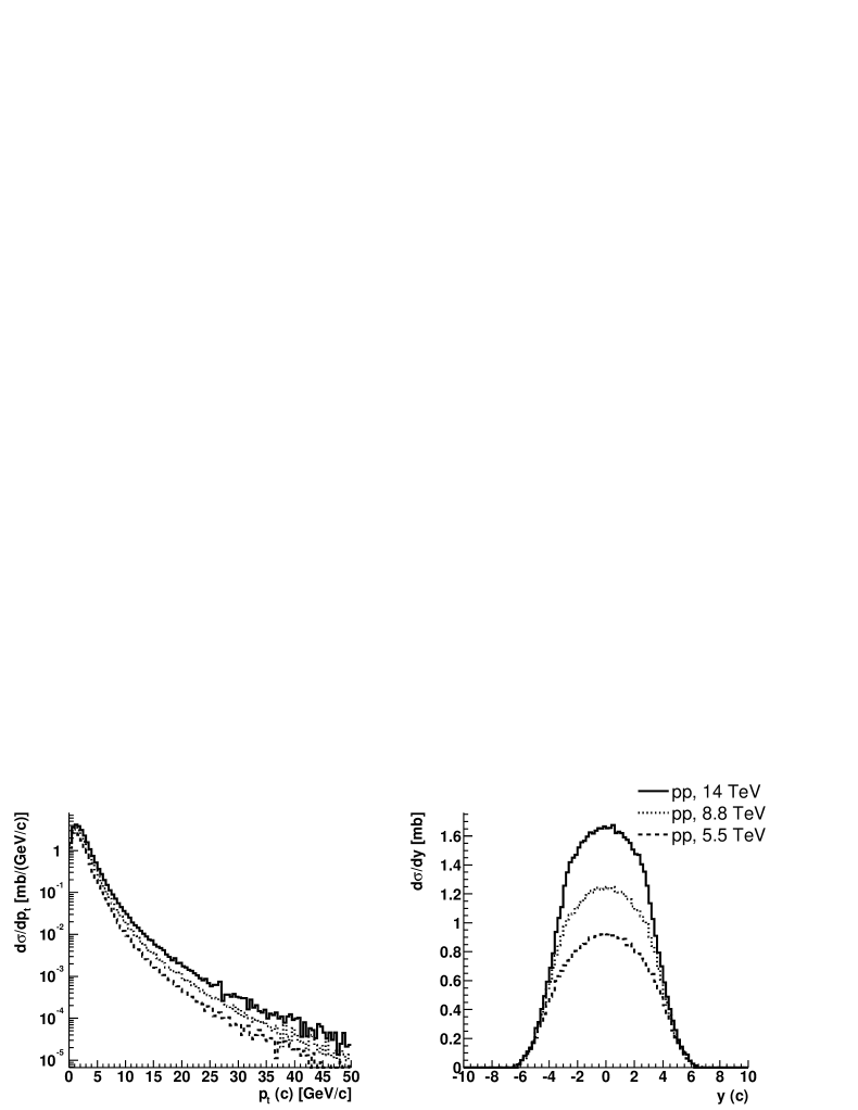
Figure 3.5: Inclusive c quark $p_{\rm t}$ and rapidity distributions obtained from the HVQMNR program, using the CTEQ 5M1 set of PDF. The distributions for Pb–Pb and p–Pb are normalized to the cross sections per nucleon–nucleon collision and they include the effects of nuclear shadowing and intrinsic $k_{\rm t}$ broadening.

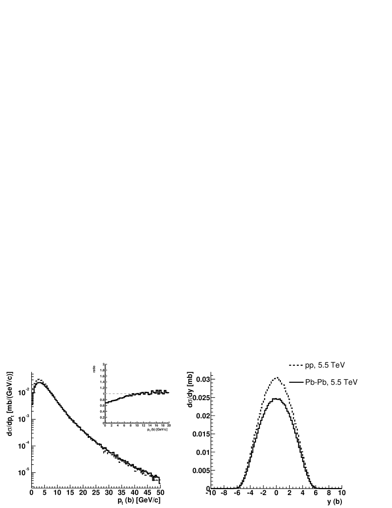
Figure 3.6: Inclusive b quark $p_{\rm t}$ and rapidity distributions obtained from the HVQMNR program, using the CTEQ 5M1 set of PDF. The distributions for Pb–Pb and p–Pb are normalized to the cross sections per nucleon–nucleon collision and they include the effects of nuclear shadowing and intrinsic $k_{\rm t}$ broadening.

3.4 Heavy quark production in Monte Carlo event generators

The program used for the NLO calculations reported in the previous sections is not well suited to be included in a simulation, since it is not an event generator and it does not provide parton kinematics. On the other hand, widely used event generators, like PYTHIA [57] and HERWIG [70], are exact only at leading order, when only the pair production processes ($q\overline{q}\to Q\overline{Q}$ and $gg\to Q\overline{Q}$) are included. Higher-order contributions are included in these generators in the parton shower approach (see e.g. Ref. [71]). This model is not exact at next-to-leading order, but it reproduces some aspects of the multiple-parton-emission phenomenon. In the following we will concentrate on the PYTHIA event generator; the version we have used is PYTHIA 6.150. We have also investigated heavy quark production in HERWIG, observing an incorrect behaviour in the final kinematical distributions of both c and b quarks. We, therefore, concluded that HERWIG is not suitable for heavy quark simulations at LHC energies. More details can be found in Ref. [65].

In PYTHIA, the processes giving rise to contributions above leading order, see Section 2.1, like flavour excitation ($qQ\rightarrow qQ$ and $gQ\rightarrow gQ$) and gluon splitting ($g\rightarrow Q\overline{Q}$), are calculated using a massless matrix element. As a consequence the cross sections for these processes diverge as $p_{\rm t}^{\rm hard}$ vanishes. These divergences are regularized by putting a lower cut-off on $p_{\rm t}^{\rm hard}$. The value of the minimum $p_{\rm t}^{\rm hard}$ cut has a large influence on the heavy flavour cross section at low $p_{\rm t}$, a region of prime interest for ALICE physics and covered by the ALICE acceptance. Our approach was, therefore, to tune the PYTHIA parameters in order to reproduce as well as possible the NLO predictions (HVQMNR). We used PYTHIA with the option MSEL=1, that allows to switch on one by one the different processes (see Appendix B for more details). The main parameter we tuned is the lower $p_{\rm t}^{\rm hard}$ limit. In this procedure we compared the following distributions of the bare quarks:

• inclusive $p_{\rm t}$ and rapidity distributions of the quark (antiquark);

• mass of the pair: $M(Q\overline{Q})=\sqrt{(E_{Q}+E_{\overline{Q}})^{2}-(\vec{p}_{Q}+\vec{p}_{\overline{Q}})^{2}}$, where $E_{Q}=\sqrt{m_{Q}^{2}+p_{Q}^{2}}$ is the quark energy;

• $p_{\rm t}$ of the pair, defined as the projection on the plane normal to the beam axis of the $Q\overline{Q}$ total momentum;

• angle $\Delta\phi$ between the quark and the antiquark in the plane normal to the beam axis.

In the simulations for Pb–Pb collisions at $\sqrt{s_{\scriptscriptstyle{{\rm NN}}}}=5.5\leavevmode\nobreak\ \mathrm{TeV}$ the parton distribution functions used are the CTEQ 4L, modified for nuclear shadowing using the EKS98 [33] parameterization. We verified that the results given by the CTEQ 4 set lie in between the ones obtained with the more recent CTEQ 5 and MRST sets for all the relevant kinematical quantities.

The overall normalization was set to the value of the cross sections obtained for proton–proton with shadowing (second row of Table 3.3).

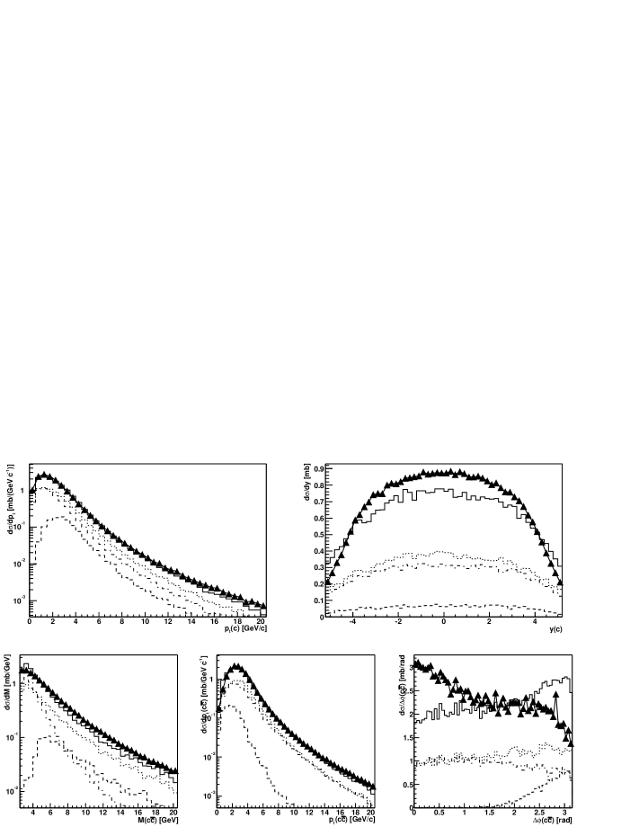
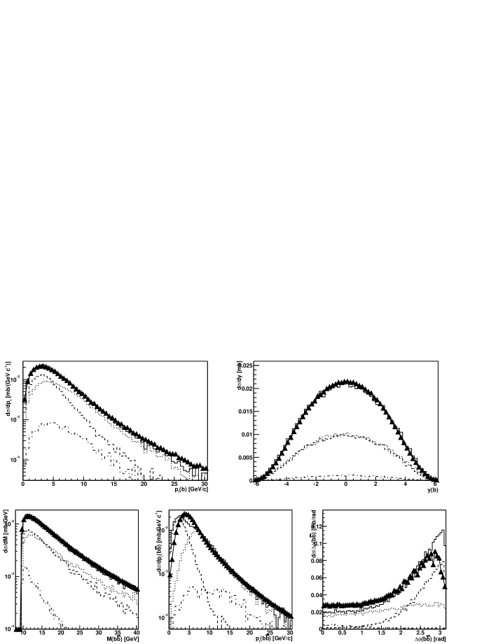
Figure 3.7: Comparison between charm production in Pb–Pb collisions at $\sqrt{s_{\scriptscriptstyle{{\rm NN}}}}=5.5\leavevmode\nobreak\ \mathrm{TeV}$ in the NLO calculation by Mangano, Nason, Ridolfi and in PYTHIA with parameters tuned as described in the text. The triangles show the NLO calculation, the solid histogram corresponds to the PYTHIA total production. The individual PYTHIA contributions are pair production (dashed), flavour excitation (dotted) and gluon splitting (dot-dashed).

Figure 3.8: Equivalent of Fig. 3.8 for beauty production.

Figure 3.9: Comparison between charm production in pp collisions at $\sqrt{s}=14\leavevmode\nobreak\ \mathrm{TeV}$ in the NLO calculation by Mangano, Nason, Ridolfi and in PYTHIA with parameters tuned as described in the text. The triangles show the NLO calculation, the solid histogram corresponds to the PYTHIA total production. The individual PYTHIA contributions are pair production (dashed), flavour excitation (dotted) and gluon splitting (dot-dashed).

Figure 3.10: Equivalent of Fig. 3.10 for beauty production.

The results of the tuning are shown in Figs. 3.8 and 3.8, where the distributions from PYTHIA and the NLO calculation are compared. The PYTHIA results are scaled to give the same total cross section as the NLO calculation. Despite the fundamental differences between the two models, the agreement is relatively good. However, significant discrepancies are present, especially in the $\Delta\phi$ distribution for $\mathrm{c\overline{c}}$ pairs.

A similar tuning of the PYTHIA event generator was done also for the production of $\mathrm{c\overline{c}}$ and $\mathrm{b\overline{b}}$ pairs in pp collisions at $\sqrt{s}=14\leavevmode\nobreak\ \mathrm{TeV}$. The same set of parton distribution functions (CTEQ 4L) was used, without the modification for nuclear shadowing. Results are shown in Figs. 3.10 and 3.10. The largest difference with the results obtained for the Pb–Pb case is a worse description of the rapidity distribution of charm quarks. This is due to a feature of the parameterizations of the parton distribution functions: most of them, including CTEQ 4, are valid only down to $x=10^{-5}$; below this value the behaviour depends on the implementation of the specific parameterization but has no physical meaning (e.g. for the CTEQ 4 the gluon density $g(x)$ is kept constant at $g(10^{-5})$). The rapidity range in which the evolution of the parton distribution functions is reliable depends on the c.m.s. energy; for charm production at $\sqrt{s}=5.5\leavevmode\nobreak\ \mathrm{TeV}$ (14 $\mathrm{TeV}$) this range is found to be $|y|<4.3$ ($|y|<3.4$), using equation (1.8) with $x_{1}>10^{-5}$ and $x_{2}>10^{-5}$.

The values of the PYTHIA parameters obtained from the tuning are reported in Appendix B.

3.5 Hadron yields and distributions

For the hadronization of heavy quarks we used the default Lund string fragmentation model [71] included in PYTHIA (JETSET package). The total yield and the rapidity density d$N$/d$y$ in the central region for hadrons with open charm and beauty in Pb–Pb at 5.5 $\mathrm{TeV}$ ($5\%\leavevmode\nobreak\ \sigma^{\rm tot}$ centrality selection), pp at 14 $\mathrm{TeV}$ and p–Pb at $8.8\leavevmode\nobreak\ \mathrm{TeV}$ are summarized in Tables 3.8, 3.8 and 3.8, respectively. The rapidity densities are calculated in $-1<y_{\rm lab}<1$, corresponding to $-1.47<y_{\rm c.m.s.}<0.53$ for p–Pb and $-0.53<y_{\rm c.m.s.}<1.47$ for Pb–p. No dependence of the relative hadron abundances on the centre-of-mass energy is observed.

Table 3.6: Total yield and average rapidity density for $|y|<1$ for hadrons with charm and beauty in Pb–Pb collisions at $\sqrt{s_{\scriptscriptstyle{{\rm NN}}}}=5.5\leavevmode\nobreak\ \mathrm{TeV}$. The values reported correspond to a centrality selection of $5\%\leavevmode\nobreak\ \sigma^{\rm tot}$.

Particle	Yield	$\langle$d$N$/d$y\rangle_{|y|<1}$	Particle	Yield	$\langle$d$N$/d$y\rangle_{|y|<1}$
${\rm D^{0}}$	68.9	6.87	${\rm B^{0}}$	1.86	0.273
${\rm\overline{D}^{0}}$	71.9	6.83	${\rm\overline{B}^{0}}$	1.79	0.262
${\rm D^{+}}$	22.4	2.12	${\rm B^{+}}$	1.82	0.251
${\rm D^{-}}$	22.2	2.00	${\rm B^{-}}$	1.83	0.270
${\rm D_{s}^{+}}$	14.1	1.30	${\rm B_{s}^{0}}$	0.53	0.077
${\rm D_{s}^{-}}$	12.7	1.22	${\rm\overline{B}_{s}^{0}}$	0.53	0.082
${\rm\Lambda_{c}^{+}}$	9.7	1.18	${\rm\Lambda_{b}^{0}}$	0.36	0.050
${\rm\overline{\Lambda_{c}}^{-}}$	8.2	0.85	${\rm\overline{\Lambda_{b}}^{0}}$	0.31	0.047

Table 3.7: Total yield and average rapidity density for $|y|<1$ for hadrons with charm and beauty in pp collisions at $\sqrt{s}=14\leavevmode\nobreak\ \mathrm{TeV}$.

Particle	Yield	$\langle$d$N$/d$y\rangle_{|y|<1}$	Particle	Yield	$\langle$d$N$/d$y\rangle_{|y|<1}$
${\rm D^{0}}$	0.0938	0.0098	${\rm B^{0}}$	0.00294	0.00043
${\rm\overline{D}^{0}}$	0.0970	0.0098	${\rm\overline{B}^{0}}$	0.00283	0.00041
${\rm D^{+}}$	0.0297	0.0029	${\rm B^{+}}$	0.00287	0.00040
${\rm D^{-}}$	0.0290	0.0029	${\rm B^{-}}$	0.00289	0.00043
${\rm D_{s}^{+}}$	0.0186	0.0018	${\rm B_{s}^{0}}$	0.00084	0.00012
${\rm D_{s}^{-}}$	0.0176	0.0020	${\rm\overline{B}_{s}^{0}}$	0.00084	0.00013
${\rm\Lambda_{c}^{+}}$	0.0113	0.0013	${\rm\Lambda_{b}^{0}}$	0.00057	0.00008
${\rm\overline{\Lambda_{c}}^{-}}$	0.0110	0.0013	${\rm\overline{\Lambda_{b}}^{0}}$	0.00049	0.00008

Table 3.8: Total yield and average rapidity density for $|y_{\rm lab}|<1$ for hadrons with charm and beauty in p–Pb collisions at $\sqrt{s_{\scriptscriptstyle{{\rm NN}}}}=8.8\leavevmode\nobreak\ \mathrm{TeV}$.

Particle	Yield	$\langle$d$N$/d$y\rangle_{|y_{\rm lab}|<1}$	Particle	Yield	$\langle$d$N$/d$y\rangle_{|y_{\rm lab}|<1}$
${\rm D^{0}+\overline{D}^{0}}$	0.926	0.096	${\rm B^{0}+\overline{B}^{0}}$	0.0221	0.0030
${\rm D^{+}+D^{-}}$	0.293	0.030	${\rm B^{+}+B^{-}}$	0.0221	0.0030
${\rm D_{s}^{+}+D_{s}^{-}}$	0.176	0.018	${\rm B_{s}^{0}+\overline{B}_{s}^{0}}$	0.0064	0.0009
${\rm\Lambda_{c}^{+}+\overline{\Lambda_{c}}^{-}}$	0.118	0.012	${\rm\Lambda_{b}^{0}+\overline{\Lambda_{b}}^{0}}$	0.0041	0.0005

It is interesting to notice the large ratio of the neutral-to-charged D meson yields: $N({\rm D^{0}})/N({\rm D^{+}})\simeq 3.1$. In PYTHIA, charm quarks are assumed to fragment to D (spin singlets: $J=0$) and D^∗ (spin triplets: $J=1$) mesons according to the number of available spin states; therefore, $N({\rm D^{0}}):N({\rm D^{+}}):N({\rm D^{*0}}):N({\rm D^{*+}})=1:1:3:3$. Then, the resonances D^∗ are decayed to D mesons according to the branching ratios. The difference between neutral and charged D mesons arises here: due to the slightly larger ($\approx 4\leavevmode\nobreak\ \mathrm{MeV}$) mass of the D⁺, the D^∗+ decays preferably to $\mathrm{D^{0}}$ and the D^∗0 decays exclusively to $\mathrm{D^{0}}$. We have [60]:

$$\begin{array}[]{rcl}\displaystyle\frac{N({\rm D^{0}})}{N({\rm D^{+}})}&=&\displaystyle\frac{N({\rm D^{0}_{primary}})+N({\rm D^{*+}})\times BR({\rm D^{*+}\to D^{0}})+N({\rm D^{*0}})\times BR({\rm D^{*0}\to D^{0}})}{N({\rm D^{+}_{primary}})+N({\rm D^{*+}})\times BR({\rm D^{*+}\to D^{+}})+N({\rm D^{*0}})\times BR({\rm D^{*0}\to D^{+}})}\\ &=&\displaystyle\frac{1+3\times 0.68+3\times 1}{1+3\times 0.32+3\times 0}\\ &=&3.08.\end{array}$$ (3.17)

We chose to use the relative abundances given by PYTHIA, although, experimentally, the fraction $\mbox{$\mathrm{D^{0}}$}/{\rm D^{+}}$ was found to be lower than 3. The value measured in $e^{+}e^{-}$ collisions at LEP by the ALEPH Collaboration is $\approx 2.4$ [72]. This would reduce by about 6% the expected yield for the $\mathrm{D^{0}}$ mesons.

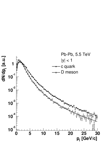
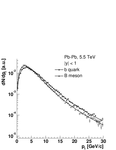
Figure 3.11: Transverse momentum distributions at mid-rapidity for heavy quarks and mesons in Pb–Pb at 5.5 TeV. The distributions are normalized to the same integral in order to compare their shapes.

Figure 3.11 presents the transverse momentum distributions at mid-rapidity ($|y|<1$) for c quarks and for D mesons (left panel) and for b quarks and B mesons (right panel), in Pb–Pb at 5.5 $\mathrm{TeV}$. For $p_{\rm t}>0$ and $|y|<1$, we have, on average, $p_{\rm t}^{\rm D}\simeq 0.75\,p_{\rm t}^{\rm c}$ and $p_{\rm t}^{\rm B}\simeq 0.85\,p_{\rm t}^{\rm b}$. The shape of the transverse momentum distributions for D and B mesons was fitted to the following expression:

$$\frac{1}{p_{\rm t}}\frac{{\rm d}N}{{\rm d}p_{\rm t}}\propto\left[1+\left(\frac{p_{\rm t}}{p_{\rm t}^{0}}\right)^{2}\right]^{-n}.$$ (3.18)

The $p_{\rm t}$ distributions were studied also for pp at 14 TeV and for p–Pb at 8.8 TeV. The results of the fits are reported in Table 3.9, together with the average $p_{\rm t}$ of D and B mesons in the different conditions. The average $p_{\rm t}$ does not depend strongly on the colliding system and on the energy in the centre of mass. On the other hand, we remark that $\left\langle p_{\rm t}\right\rangle$ is larger by $\approx 10\%$ at mid-rapidity than in the forward region ($2.5<y<4$). These two regions correspond to the acceptance of the ALICE detector: barrel, $|\eta|<0.9$, and forward muon arm, $2.4<\eta<4$ (more details on the structure of the detector are given in Chapter 4).

Finally, we show in Fig. 3.12 the $p_{\rm t}$ distributions of kaons and pions from the decay ${\rm D^{0}\to K^{-}\pi^{+}}$ (and charge conjugate) in Pb–Pb at $5.5\leavevmode\nobreak\ \mathrm{TeV}$: the average $p_{\rm t}$ is $1.2\leavevmode\nobreak\ \mathrm{GeV}/c$ for the kaons and $1.1\leavevmode\nobreak\ \mathrm{GeV}/c$ for the pions. For kaons and pions in $|\eta|<0.9$ (ALICE barrel acceptance) the average momenta are $\left\langle p_{\rm K}\right\rangle=1.5\leavevmode\nobreak\ \mathrm{GeV}/c$ and $\left\langle p_{\pi}\right\rangle=1.3\leavevmode\nobreak\ \mathrm{GeV}/c$; thus, they are with good approximation relativistic, since $\left\langle E_{\rm K}\right\rangle/\left\langle p_{\rm K}\right\rangle\simeq 1.05$ and $\left\langle E_{\pi}\right\rangle/\left\langle p_{\pi}\right\rangle\simeq 1.01$.

Table 3.9: Parameters derived from the fit of the $p_{\rm t}$ distributions of D and B mesons to the expression (3.18) and average value of $p_{\rm t}$ for these particles.

Particle	System	$\sqrt{s_{\scriptscriptstyle{{\rm NN}}}}$ [TeV]	$p_{\rm t}^{0}\leavevmode\nobreak\ [\mathrm{GeV}/c]$	$n$	$\left\langle p_{\rm t}\right\rangle[\mathrm{GeV}/c]$
	pp	14	2.04	2.65	1.85
D	p–Pb	8.8	2.09	2.72	1.83
($|y_{\rm lab}|<1$)	Pb–Pb	5.5	2.12	2.78	1.81
	pp	14	2.18	3.04	1.67
D	p–Pb	8.8	2.22	3.11	1.66
($2.5<y_{\rm lab}<4$)	Pb–Pb	5.5	2.25	3.17	1.64
	pp	14	6.04	2.88	4.90
B	p–Pb	8.8	6.08	2.90	4.89
($|y_{\rm lab}|<1$)	Pb–Pb	5.5	6.14	2.93	4.89
	pp	14	6.45	3.54	4.24
B	p–Pb	8.8	6.49	3.56	4.24
($2.5<y_{\rm lab}<4$)	Pb–Pb	5.5	6.53	3.59	4.24

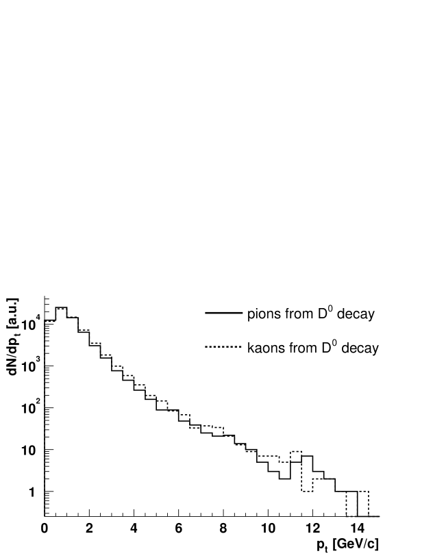
Figure 3.12: Transverse momentum distributions for kaons and pions from $\mathrm{D^{0}}$ meson decays in Pb–Pb at 5.5 TeV.

Chapter 4 The ALICE experiment at the LHC

This chapter is devoted to the description of ALICE, the dedicated heavy ion experiment at the Large Hadron Collider. We start by presenting the ALICE layout and its different sub-systems, with particular emphasis on the detectors of the barrel, in the central rapidity region, which are employed for the measurement of hadronic observables (Section 4.1). In Section 4.2 we describe event simulation and reconstruction in ALICE. After a brief overview of the employed event generators, of the detector response simulation and of the track reconstruction strategy, we concentrate on the tracking performance, in terms of efficiency and momentum resolution, in different multiplicity environments. Finally, we discuss some parameters of the LHC heavy ion and proton beams which are relevant for the study presented in this thesis (Section 4.3).

4.1 The ALICE detector

ALICE is conceived as a general-purpose detector, in which most of the hadrons, leptons and photons produced in the interaction can be measured and identified.

The requirement of the combined capability to track and identify particles of very low up to fairly high $p_{\rm t}$, and to reconstruct the decays of hyperons and D and B mesons in an environment with charged particle multiplicities up to 8000/unit rapidity at mid-rapidity, has led to a unique design, with a very different optimization with respect to the pp-dedicated experiments at the LHC.

4.1.1 Detector layout

The general ALICE layout is shown in Fig. 4.1.

It consists of a central detector ($|\eta|<0.9$) covering the full azimuth, where hadrons, electrons and photons are measured, and a forward muon arm ($2.4<\eta<4$) [73, 74, 75]. We define here the ALICE global reference frame: it has $z$ axis parallel to the beam direction and pointing towards the muon arm, $x$ and $y$ axes in the plane transverse to the beam direction.

The central detector is embedded in a large solenoidal magnet with a weak field of $<0.5$ T, parallel to $z$, and it consists of the Inner Tracking System (ITS) with six layers of high-resolution silicon detectors, the cylindrical Time Projection Chamber (TPC), a Transition Radiation Detector (TRD) for electron identification, a barrel Time of Flight (TOF), a small-area ring imaging Cherenkov detector at large distance for the identification of high-momentum particles (High Momentum Particle Identifier - HMPID), and a single-arm electromagnetic calorimeter of high-density crystals (Photon Spectrometer - PHOS).

The design of the tracking system was primarily driven by the requirement for safe and robust track finding. It uses mostly three-dimensional hit information and dense tracking with many points (TPC). The detection of hyperons, and even more of D and B mesons, requires in addition a high-resolution vertex detector close to the beam pipe (ITS).

The field strength is a compromise between momentum resolution and low momentum acceptance. The momentum cut-off should be as low as possible ($\simeq 100\leavevmode\nobreak\ \mathrm{MeV}/c$), in order to detect the decay products of low-$p_{\rm t}$ hyperons. At high $p_{\rm t}$ the magnetic field determines the momentum resolution, which is essential for the study of jet quenching and high-$p_{\rm t}$ leptons. The ideal choice for hadronic physics, maximizing reconstruction efficiency, would be around $0.2$ T, while for the high-$p_{\rm t}$ observables the maximum field the magnet can produce, $0.5$ T, would be the best choice. Since the high-$p_{\rm t}$ observables are limited by statistics, ALICE will run mostly with the higher field option.

The beam pipe has the smallest possible thickness (in terms of the radiation length, $X_{0}$) to minimize the multiple scattering undergone by the particles produced in the collision. It is built in beryllium (usually chosen for its low atomic number, i.e. low radiation length) and it has an outer radius of 3 cm and a thickness of 0.8 mm, corresponding to 0.3% of $X_{0}$.

Figure 4.1: Layout of the ALICE detector.

The muon spectrometer is designed to measure the production of the complete spectrum of heavy quark resonances, namely J/$\psi$ and $\psi^{\prime}$, $\Upsilon$, $\Upsilon^{\prime}$ and $\Upsilon^{\prime\prime}$. It is constructed of an absorber very close to the vertex followed by a spectrometer with a dipole magnet and, finally, an iron wall to select the muons.

The set-up is completed by a forward photon counting detector (Photon Multiplicity Detector - PMD) and a multiplicity detector (Forward Multiplicity Detector - FMD) covering the forward rapidity region, that, in conjunction with the ITS allows the measurement of the charged multiplicity in the range $-3.4<\eta<5.1$.

A system of scintillators (V0 detector) and quartz counters (T0 detector) provide fast trigger signals.

The collision centrality is determined by measuring the energy (and, thus, the number) of spectator nucleons, that lay outside the transverse superposition region of the two colliding nuclei and continue to propagate along the beam direction. Owing to their different Z/A values, it is possible to separate in space the neutron and proton spectators and the beam particles (Z/A $\simeq 0.4$ for Pb beams) by means of the first LHC dipole. Therefore, the neutron and proton spectators are detected in two distinct calorimeters (Zero Degrees Calorimeters - ZDC), made respectively of tantalum and brass with embedded quartz fibers, located on both sides of the interaction region $\approx 90\leavevmode\nobreak\ \mathrm{m}$ downstream in the machine tunnel.

In the following, we describe the sub-systems of ALICE which are employed for the measurement of open charm particles in hadronic decay channels: the TPC and the ITS, that allow tracking and reconstruction of the interaction vertex and of secondary vertices; the TOF detector, that provides particle identification for hadrons over the full geometrical acceptance of the central barrel.

4.1.2 Inner Tracking System (ITS)

The task of the inner tracker is to provide:

• primary and secondary vertex reconstruction with the high resolution that is required for the detection of hyperons and particles with open charm and open beauty;

• tracking and identification of low-$p_{\rm t}$ particles which are strongly bent by the magnetic field and do not reach the TPC;

• improved momentum resolution for the higher-$p_{\rm t}$ particles which also traverse the TPC.

These goals are achieved with a silicon detector structured in six cylindrical layers, from the inside to the outside: two layers of Silicon Pixel Detectors (SPD), located at $r=4$ and $7\leavevmode\nobreak\ \mathrm{cm}$; two layers of Silicon Drift Detectors (SDD), $r=14$ and $24\leavevmode\nobreak\ \mathrm{cm}$; two layers of Silicon Strip Detectors (SSD), $r=39$ and $44\leavevmode\nobreak\ \mathrm{cm}$. A general view of the ITS is shown in Fig. 4.2 and the main parameters of each of the three detector types are reported in Table 4.1.

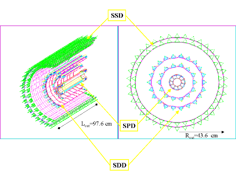
Figure 4.2: Layout of the ITS.

Table 4.1: Parameters of the various detector types of the ITS. The occupancy is calculated for the maximum expected particle density in Pb–Pb collisions at the LHC (${\rm d}N_{\rm ch}/{\rm d}y=8000$).

Parameter		Silicon Pixel	Silicon Drift	Silicon Strip
Radius (inner layer)	[cm]	4	14	39
Radius (outer layer)	[cm]	7	24	44
Cell size ($r\phi\times z$)	[$\mathrm{\mu m}^{2}$]	$50\times 425$	$150\times 300$	$95\times 40000$
Spatial precision ($r\phi\times z$)	[$\mathrm{\mu m}^{2}$]	$12\times 120$	$38\times 28$	$20\times 830$
Readout channels	[k]	9835	133	2719
Av. occup. (inner layer)	[%]	2.1	2.5	4
Av. occup. (outer layer)	[%]	0.6	1.0	3.3
Thickness per layer	[% of $X_{0}$]	1.24	0.95	0.90

The high particle density expected in heavy ion collisions and the requirement for optimal reconstruction of secondary vertices, have dictated the choice of silicon detectors with high granularity and true two-dimensional readout for the four innermost planes.

The pixel detectors, in layers 1 and 2, with a cell (pixel) size of $50(r\phi)\times 425(z)\leavevmode\nobreak\ \mathrm{\mu m}^{2}$, allow excellent position resolution in an environment where the track density may exceed 50 tracks/$\mathrm{cm}^{2}$. For the two intermediate layers, 3 and 4, silicon drift detectors have been selected, since they couple a very good multi-track capability to the information on the specific energy loss (with the two-dimensional analog readout).

At larger radii, layers 5 and 6, the requirements in terms of granularity are less stringent, therefore double-sided silicon micro-strip detectors are used. Double-sided micro-strips have been selected rather than single-sided ones because they offer the possibility to correlate the pulse height read out from the two sides, thus helping to resolve ambiguities inherent in the use of detectors with one-dimensional readout. This aspect is very important for the connection of tracks from the TPC to the ITS.

With the drift and the strip detectors, the four outer layers have analog readout. This allows to apply a truncated-mean method (requiring at least four measurements) for the estimate of the d$E$/d$x$ and gives the ITS a stand-alone capability as low-momentum particle spectrometer, in the 1/$\beta^{2}$ region of the Bethe-Bloch curve [60].

The pseudorapidity coverage of the ITS is $|\eta|<0.9$ for collisions with vertex located within the length of the interaction diamond, i.e. $-5.3<z<5.3\leavevmode\nobreak\ \mathrm{cm}$ along the beam direction. The first layer of pixel detectors has a more extended coverage ($|\eta|<1.98$) to provide, together with the forward multiplicity detectors, a continuous coverage in rapidity for the measurement of charged multiplicity.

The track momentum and position resolutions for particles with small transverse momenta are dominated by multiple scattering effects. Therefore, the minimization of the material thickness is an absolute priority in the ITS, which is the first detector crossed by the particles produced in the collision. In the two innermost layers, both the pixel sensor and the electronics chip are $200\leavevmode\nobreak\ \mathrm{\mu m}$ thick, for a total silicon budget of $400\leavevmode\nobreak\ \mathrm{\mu m}$ per layer. Including also the carbon-fiber supports and the cooling system, the average material per layer traversed by a straight track perpendicular to the beam line corresponds to $1.2\%$ of $X_{0}$. Also the drift and strip layers have a similar material budget, so that the total thickness of the ITS corresponds to $\approx\leavevmode\nobreak\ 6\%$ of $X_{0}$.

The improvement of the momentum measurement, obtained when the tracks reconstructed in the TPC are prolonged in the ITS, is discussed in Section 4.2.3. The performance of the ITS for the issues related to the reconstruction of secondary vertices (namely, track position resolution and primary vertex reconstruction) was studied in detail in the scope of this thesis and it is described in a dedicated chapter (Chapter 5).

4.1.3 Time Projection Chamber (TPC)

The TPC is the main tracking detector in ALICE: it provides track finding, momentum measurement and particle identification via d$E$/d$x$.

A view of the detector is shown in Fig. 4.3 (right). The TPC has an inner radius of 80 cm, given by the maximum acceptable hit density (0.1 cm^-2), and an outer radius of 250 cm, given by the length required for a d$E$/d$x$ resolution better than $10\%$, necessary for particle identification. The total active length of 500 cm allows the acceptance in the pseudorapidity range $|\eta|<0.9$.

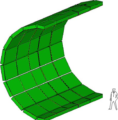
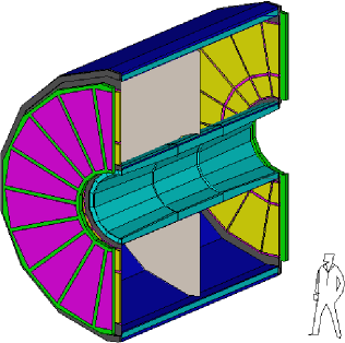
Figure 4.3: A view of the ALICE Time of Flight (left) and Time Projection Chamber (right) how they are described in the detector simulation framework. For graphical clearness only half of the azimuthal coverage of the detectors is shown.

The gas mixture Ne/CO₂ (90%/10%) is optimized for drift velocity, low electron diffusion and low radiation length.

The TPC readout chambers are multi-wire proportional chambers with cathode-pad readout. The readout planes at the two ends of the large drift volume ($88\leavevmode\nobreak\ \mathrm{m}^{3}$) are azimuthally segmented in 18 sectors, each covering an angle of $20^{\circ}$. The non-active region between two adjacent sectors is 2.7 cm wide, implying an azimuthal acceptance of $\approx 90\%$ for straight tracks originating from the interaction point. The radial thickness of the detector is of $3.5\%$ of $X_{0}$ at central rapidity and grows to $\approx 40\%$ towards the acceptance edges.

Track reconstruction strategy and performance in the TPC in the high-multiplicity environment of heavy ion collisions and in pp collisions will be described in detail in Section 4.2.3.

4.1.4 Particle identification system

One of the distinctive features of ALICE is the particle identification capability, which is realized using a number of different techniques.

Charged hadron identification is provided over the full barrel acceptance ($|\eta|<0.9$) by the combination of (a) d$E$/d$x$ measurement in the four outer layers of the ITS and in the TPC, for momenta up to $\simeq 0.5\leavevmode\nobreak\ \mathrm{GeV}/c$, with (b) a barrel Time of Flight at $r=370\leavevmode\nobreak\ \mathrm{cm}$, in the range $0.5<p<2.5\leavevmode\nobreak\ \mathrm{GeV}/c$. Electron are separated from pions for $p_{\rm t}>1\leavevmode\nobreak\ \mathrm{GeV}/c$ by means of a dedicated Transition Radiation Detector and by exploiting the relativistic rise of the specific energy loss measured in the TPC. A smaller-area ring imaging Cherenkov detector (HMPID), covering about $15\%$ of the acceptance of the ALICE central detectors, allows the separation of hadrons up to higher momenta ($\pi$/K up to $3\leavevmode\nobreak\ \mathrm{GeV}/c$ and K/p up to $5\leavevmode\nobreak\ \mathrm{GeV}/c$).

Photons and neutral pions are identified in the small-acceptance electromagnetic calorimeter PHOS.

Here we describe in detail only the TOF detector. For the other detectors see Refs. [73, 75].

Time of Flight detector (TOF)

The TOF barrel is positioned outside the TRD and has an internal radius of $370\leavevmode\nobreak\ \mathrm{cm}$ and an external radius of $399\leavevmode\nobreak\ \mathrm{cm}$. Its task is to provide hadron separation in the momentum range from $0.5\leavevmode\nobreak\ \mathrm{GeV}/c$, where the d$E$/d$x$ technique is no longer effective, to about $2.5\leavevmode\nobreak\ \mathrm{GeV}/c$. PID in this momentum range allows the study of the kinematical distributions of the different particle types on an event-by-event basis in heavy ion collisions. Moreover, given the large mass of the charm quark, the decay products of D mesons have typical momenta of the order of $1$-$2\leavevmode\nobreak\ \mathrm{GeV}/c$; therefore, the Time of Flight, with K/$\pi$ separation up to $2.5\leavevmode\nobreak\ \mathrm{GeV}/c$, is very effective for the reconstruction of exclusive decays of D mesons in hadronic channels.

The time-of-flight is measured using the technology of the Multi-gap Resistive Plate Chambers (MRPC). The RPC is a gaseous detector with resistive electrodes, which quench the streamers so that they do not initiate a spark breakdown.

The TOF MRPC design consists of a double stack with $2\times 5$ gaps. The basic unit is a MRPC pad of size $3.5\times 2.5\leavevmode\nobreak\ \mathrm{cm}^{2}$; the pads are organized in large modules and the full barrel counts 18 (in $r\phi$) $\times$ 5 (along $z$) modules, for a total active area of $\approx 140\leavevmode\nobreak\ \mathrm{m}^{2}$. A view of the detector is shown in Fig. 4.3 (left).

The MRPC resolution has been measured to be in the $50$-$60$ ps range, with efficiency above $99\%$. Including the other sources of timing errors, the overall resolution is estimated to be $\approx 120$ ps.

In Chapter 6 the PID performance of the detector will be presented, along with the TOF PID strategy optimized for the detection of charm mesons in Pb–Pb and in pp collisions.

4.2 Event simulation and reconstruction

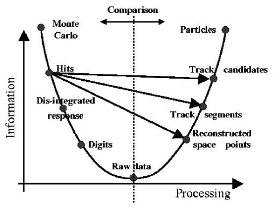
Figure 4.4: Schematic representation of the data processing chain.

The ALICE off-line framework, AliRoot [76], is described in detail in Ref. [77]. This framework, based on the Object Oriented / C++ environment of ROOT [78], allows to reconstruct and analyze physics data coming from simulations and real interactions. The role of the framework can be graphically represented as shown in Fig. 4.4. Events are generated via Monte Carlo simulation programs, generators and detector simulation, and are then transformed into the format produced by the detector (raw data). Here we have a minimum of the physics information. At this point, the reconstruction and analysis chain is used to evaluate the detector and the physics performance, and most of the initial information on the generated event can be retrieved (e.g. particle ID and kinematics, event topology). In the next paragraphs we will follow from the left to the right the parabola in Fig. 4.4 and detail the aspects which are relevant to the studies reported in this thesis.

4.2.1 Event generators

We briefly describe here some relevant features of the Monte Carlo event generators that were used for the simulation of pp minimum-bias collisions (PYTHIA) and of Pb–Pb central collisions (HIJING) at LHC energies.

PYTHIA

The PYTHIA [57] event generator, was introduced in Section 3.4, where we have reported how its parameters were tuned in order to reproduce the $p_{\rm t}$ distributions for heavy quarks as predicted by NLO pQCD.

PYTHIA was also employed for the production of a large sample of pp non-diffractive interactions at $\sqrt{s}=14\leavevmode\nobreak\ \mathrm{TeV}$ that served as background (or, more appropriately, underlying) events for the study on the detection of D mesons in pp. To this purpose, the version 6.150 of the program was used with the CTEQ 4L set of PDF and with the parameters tuned in order to reproduce the multiplicity of all available collider data [79]. As detailed in Ref. [79], the main parameter tuned is the low-$p_{\rm t}$ cut-off, $p_{\rm t}^{\rm min}$, introduced in the model to regularize the dominant $2\to 2$ QCD cross sections, which diverge as $p_{\rm t}\to 0$ and drop rapidly at high $p_{\rm t}$. In order to reproduce the data, a monotonic increase of $p_{\rm t}^{\rm min}$ with $\sqrt{s}$ has to be introduced.

The predicted average charged particle rapidity density in non-diffractive inelastic pp collisions at $\sqrt{s}=14\leavevmode\nobreak\ \mathrm{TeV}$ is ${\rm d}N_{\rm ch}/{\rm d}y\approx 6$. In PYTHIA, at this energy the ratio of the non-diffractive inelastic cross section to the total inelastic cross section is $\simeq 0.7$.

For events with charm production we can expect a multiplicity higher than the average, due to the fact that heavy quarks, having a large mass, yield more particles, in their fragmentation, than light quarks and gluons. We shall discuss in detail this point in Chapter 6, where we will compare the charged particle multiplicity and the mean $p_{\rm t}$ predicted by PYTHIA for events with and without charm production.

HIJING

HIJING [80] (Heavy Ion Jet INteraction Generator) combines a QCD-inspired model of jet production with the Lund string model [71] for jet fragmentation. Binary scaling with Glauber geometry is used to extrapolate to proton–nucleus and nucleus–nucleus collisions.

Nuclear shadowing and parton energy loss are included in the HIJING model and they can be selected by the user.

The charged particle rapidity density at mid-rapidity and the total number of charged particles in the ALICE barrel acceptance ($|\eta|<0.9$) given by HIJING for central (impact parameter $b<2\leavevmode\nobreak\ \mathrm{fm}$) Pb–Pb collisions at $\sqrt{s_{\scriptscriptstyle{{\rm NN}}}}=5.5\leavevmode\nobreak\ \mathrm{TeV}$, with and without jet quenching, are reported in Table 4.2. Taking into account energy loss (quenching) leads to a factor of 2 increase in multiplicity at mid-rapidity.

Table 4.2: Charged particle multiplicity and total number of charged particles in the ALICE barrel acceptance given by HIJING for central Pb–Pb ($b<2\leavevmode\nobreak\ \mathrm{fm}$) at the LHC.

Setting	${\rm d}N_{\rm ch}/{\rm d}y$ at $y=0$	$N_{\rm ch}$ in $|\eta|<0.9$
Energy loss on	$\simeq$ 6200	$\simeq$ 10800
Energy loss off	$\simeq$ 2900	$\simeq$ 5200

For our background studies in Pb–Pb we used HIJING events with $b<2\leavevmode\nobreak\ \mathrm{fm}$ and with energy loss. This is a conservative choice, since the obtained multiplicity ${\rm d}N_{\rm ch}/{\rm d}y\approx 6000$ is close to the most pessimistic expectation for the LHC, ${\rm d}N_{\rm ch}/{\rm d}y=8000$, and about a factor 2 larger than the value predicted by the most recent analyses of RHIC results, ${\rm d}N_{\rm ch}/{\rm d}y\approx 2500$ (see Section 1.4.1).

Finally, we remark that the use of HIJING allows to keep into account all sources of physical backgrounds (e.g. decays of strange particles, that can fake the topology of a charm particle decay vertex). We will give more details on this point in Chapter 6.

4.2.2 Simulation of the detector response

After event generation, in order to produce the equivalent of the raw data (minimum of the parabola in Fig. 4.4) the following steps are necessary:

• Particle transport. The particles are transported in the material of the detector, simulating their interaction with it and the energy deposition that generates the detector response (hits). To this purpose the program GEANT3.21 [81], interfaced to AliRoot, is used. All physical processes are taken into account, including a complete description of Coulomb scattering of charged particles on atomic nuclei. The ALICE detector is described in great detail, including support structures, beam pipe and services.

• Signal generation and detector response. During this phase the detector response is generated from the energy deposition of the particles traversing it. This is the ‘ideal’ detector response, before the conversion to digital signal and the formatting of the front-end electronics are applied.

• Digitization. The detector response is digitized and formatted according to the output of the front-end electronics and the Data Acquisition System. The results should resemble closely the real data that are produced by the detector.

4.2.3 Track reconstruction

The event reconstruction procedure includes:

1. cluster finding;

2. track reconstruction;

3. reconstruction of the position of the interaction vertex.

We shall describe the reconstruction of the interaction (or primary) vertex in Chapter 5, which is dedicated to the items concerning displaced vertices identification. Here, after a brief note on cluster finding, we focus on track reconstruction and, particularly, on tracking performance.

Cluster finding

During cluster finding, the information given by the detector electronics (digits) is converted to space points, interpreted as (a) the crossing points between the tracks and the centres of the pad rows in the readout chambers, in the case of the TPC, and (b) the crossing points between the tracks and the silicon sensitive volumes, in the case of the ITS. Another important piece of information provided by the cluster finder, is the estimate of the errors of the reconstructed space points. At present, a procedure for parallel clustering and tracking in the TPC is being tested. In the high-multiplicity scenario of Pb–Pb collisions clusters from different tracks may overlap and a preliminary knowledge of the track parameters is very helpful in the cluster deconvolution.

The possibility to use a fast simulation of the detector response is implemented for many sub-systems of ALICE. The clusters are obtained directly from the hits via a parameterization of the response, in terms of efficiency and spatial resolution. The dramatic reduction in computing time (e.g. a factor $\simeq 25$ in the case of the ITS) allows the use of very high statistics in simulation studies. The clusters obtained via the fast simulation are called fast points, while those obtained from the detailed detector response are called slow points.

Track reconstruction in TPC–ITS

Due to the expected charged particle multiplicity, track finding in ALICE is a very challenging task. In the most pessimistic case, the occupancy (defined as the ratio of the number of read-out channels over threshold to the total number of channels) in the inner part of the TPC may reach 40%.

The track finding procedure developed for the barrel (ITS, TPC, TRD, TOF) is based on the Kalman filtering algorithm [82], widely used in high-energy physics experiments. The Kalman filter is a method for simultaneous track recognition and reconstruction (or, in other words, track finding and fitting) and its main property is that, being a local method, at any given point along the track it provides the optimal estimate of the track geometrical parameters at that point. For this reason it is a natural way to find the extrapolation of a track from a detector to another (for example from the TPC to the ITS or TRD). As we will explain, in the Kalman filter energy loss and multiple scattering are accounted for in a direct and simple way.

The complete chain of track reconstruction in the ALICE barrel foresees the following steps: (a) track finding in the TPC, inward (i.e. from the outer to the inner part); (b) matching to the ITS outer layer and track finding inward down to the innermost pixel layer; (c) back-propagation and refit of the track outward in ITS and TPC, up to the outer radius of the TPC; (d) matching to the TRD and track finding (outward) in the TRD; (e) matching to the TOF detector, for PID.

Here we describe only steps (a) and (b), since this is the part of the chain which was employed in the studies performed for this work.

In the Kalman filter procedure, as implemented in ALICE, a track in the magnetic field of the barrel is locally (i.e. at a certain radial position in the barrel) parameterized as an helix, identified by a state vector of 5 parameters. Two parameters describe the track geometry in the beam direction ($z$) and three in the plane transverse to the beam (also referred to as bending plane). The description of the track state is completed by the $5\times 5$ covariance matrix of the parameters, which, at any given point, contains the best estimate of the errors on the parameters and of their correlations. In the TPC tracking, the procedure starts from the searching of track seeds in the outermost pad rows of the detector, where the occupancy is lower. All pairs of points, the first on the outermost pad row and the second on the pad row which is $n$ rows closer to the interaction point, are considered. For each pair, using the two points and the primary vertex position, a first estimate of the state vector at the outermost pad row is obtained. Then, track points in the next $n$ rows are searched, and, if at least $n/2$ points are found, the candidate is saved as a track seed. Subsequently, a second seed-finding step is performed using another pair of rows. At this point the Kalman filter through the TPC starts, beginning with the tracks with lower curvature (i.e. higher $p_{\rm t}$) that are found more easily, because the effect of multiple scattering is inversely proportional to the track momentum. The algorithm proceeds with an iteration of three steps:

1. Prediction: given the state $j-1$ of the track at a certain layer, a prediction of the state $j$ is obtained by propagating the track-helix to the next layer. In this prolongation the track curvature is modified to take into account the energy loss and the covariance matrix is updated according to the multiple scattering in the material encountered by the track.

2. Filtering: after the extrapolation to the state $j$, all clusters whose coordinates are inside a suitable ‘road’ are considered, the road being defined by the track covariance matrix and by the spatial resolution of the present detector layer. For each cluster the state vector is updated and a $\chi^{2}$-increment is calculated. Then, all the possible prolongations are ‘filtered’ and the cluster that gives the minimum $\chi^{2}$-increment is assigned to the track, provided that the increment is lower than a given $\chi^{2}_{\rm max}$.

3. Update: finally the state $j$ of the track is updated using the information of the assigned cluster.

In the ITS implementation, the Kalman procedure was modified towards a more global approach. The tracks found in the TPC are used as seeds, again beginning with higher-$p_{\rm t}$ tracks. In order to find the prolongation of a TPC track inside the ITS, for each seed all clusters on the outer ITS layer which are located in the fiducial road are considered. For each of them a new candidate track is defined and propagated to the next layer, without applying any filtering. In this way, a track-tree with many candidates is built from a single TPC track, and only when the inner pixel layer is reached the filtering is applied and the candidate with the lowest $\chi^{2}$ per assigned cluster is selected. The assigned clusters are ‘removed’ and the next TPC track is considered. In this way the finding of the low-$p_{\rm t}$ tracks is facilitated, since all the clusters from the previously found tracks are not considered.

Two track finding steps are used in the ITS: the first with a constraint on the position of the primary vertex, measured by the pixel layers (see Chapter 5), to increase the efficiency for the tracks originating from the primary vertex (primary tracks); in the second step this constraint is removed in order to allow the finding of tracks coming from displaced vertices (secondary tracks, e.g. decay products of strange particles). Decay products of charm (and beauty) mesons can be considered as primary, from the point of view of track finding, since their displacement is usually lower than $1\leavevmode\nobreak\ \mathrm{mm}$. Afterwards, all found tracks are refitted without vertex constraint, in order to get an unbiased estimate of the distance from the interaction point.

In the next sections we shall present the relevant performance parameters of the track reconstruction in the TPC and in TPC–ITS. The two extremes of the multiplicity scale are considered: central Pb–Pb (${\rm d}N_{\rm ch}/{\rm d}y=6000$, HIJING) and pp collisions (${\rm d}N_{\rm ch}/{\rm d}y=6$, PYTHIA). The value of the magnetic field is 0.4 Tesla.

Tracking efficiency in pp and in Pb–Pb

Figure 4.6 presents the tracking efficiency for primary tracks in the TPC, defined as a the ratio of the number of reconstructed tracks to the number of generated tracks (the acceptance cut of the barrel, $|\eta|<0.9$, is applied to both numerator and denominator). The left panel corresponds to Pb–Pb, the right one to pp. The efficiency is shown as a function of the transverse momentum for charged pions and charged kaons separately. The large difference between kaons and pions is due to the lower mean decay length of the former —$7.5\leavevmode\nobreak\ \mathrm{m}\cdot p(\mathrm{GeV}/c)$ for kaons and $55.7\leavevmode\nobreak\ \mathrm{m}\cdot p(\mathrm{GeV}/c)$ for pions. In pp, the lower occupancy allows a higher track finding efficiency. At very high $p_{\rm t}$ (straight tracks) the inefficiency of $\sim 10\%$ is due to the non-active regions of the TPC (separation between different sectors).

Figure 4.5: Tracking efficiency in the TPC, as a function of the transverse momentum, for charged pions and kaons in Pb–Pb (left) and pp (right) events. The efficiency is defined as the ratio (in $|\eta|<0.9$) of the number of found primary tracks to the number of generated primary tracks.

Figure 4.6: Same as the previous figure, but for TPC–ITS. Six assigned clusters per track in the ITS are required.

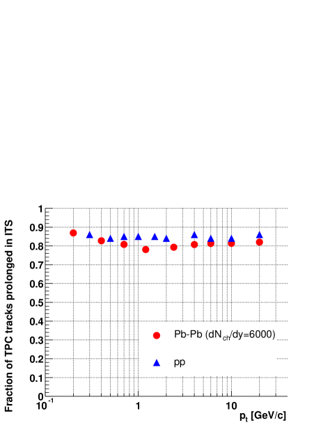
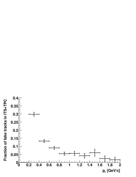
Figure 4.7: Fraction of TPC tracks prolonged to the ITS, with 6 clusters, in pp and in Pb–Pb (top) and, for Pb–Pb, fraction of ITS tracks with at least one misassigned cluster in the ITS (bottom).

Figure 4.6 shows the efficiency, defined as for the previous figure, for the system TPC–ITS. In the ITS an assigned cluster per layer is required (6 clusters in total). The average efficiency, taken into account the $p_{\rm t}$ distribution of the particles generated by PYTHIA and HIJING, is $\simeq 65\%$ ($\simeq 75\%$) for pions and $\simeq 45\%$ ($\simeq 50\%$) for kaons in Pb–Pb (pp).

The fraction of TPC tracks prolonged in the ITS is roughly the same in pp and Pb–Pb (Fig. 4.7, upper panel). However, in Pb–Pb, due to the high occupancy in the ITS layers, there is a non-negligible fraction of tracks that have at least one incorrectly-assigned cluster (fake tracks). As shown in Fig. 4.7 (lower panel), this effect is mainly restricted to low-$p_{\rm t}$ tracks ($p_{\rm t}<1\leavevmode\nobreak\ \mathrm{GeV}/c$). We will compare the quality of correctly-reconstructed and fake tracks, in terms of track position resolution, in Chapter 5.

Momentum resolution in pp and in Pb–Pb

The momentum resolution is a very important parameter for the selection of rare signals and for the measurement of their $p_{\rm t}$ distribution. In particular, we have seen (Section 2.5.1 and Appendix A) that in the case of invariant mass analyses, if the decay particles are relativistic (as in the ${\rm D^{0}\to K^{-}\pi^{+}}$ decay at LHC energies) the mass resolution is proportional to the momentum resolution. Therefore, the signal-to-background ratio is inversely proportional to the momentum resolution.

Given the importance of this parameter, we cross-checked, in a simple case, the result obtained using the detector simulation in AliRoot. The transverse momentum resolution can be approximated as a quadratic sum of a contribution due to the multiple scattering and a contribution due to the detector resolution. If the relative resolution is considered, the first contribution is a constant and the second is proportional to the transverse momentum itself [60]:

$$\frac{\sigma(p_{\rm t})}{p_{\rm t}}=K_{\rm scatt}\oplus K_{\rm meas}\cdot p_{\rm t}\equiv\sqrt{K_{\rm scatt}^{2}+K_{\rm meas}^{2}\cdot p_{\rm t}^{2}}.$$ (4.1)

If $p_{\rm t}$ is measured in a solenoidal magnetic field $B$ using uniformly distributed points with the same spatial resolution, the term $K_{\rm meas}$ should be [60]:

$$K_{\rm meas}=\frac{\sigma_{r\phi}}{0.3\,B\,\ell^{2}}\sqrt{\frac{720}{N+2}}$$ (4.2)

where $N$ is the number of points, $\sigma_{r\phi}$ is their spatial resolution in the transverse plane and $\ell$ is the lever arm of the arc between the first and the last measured point.

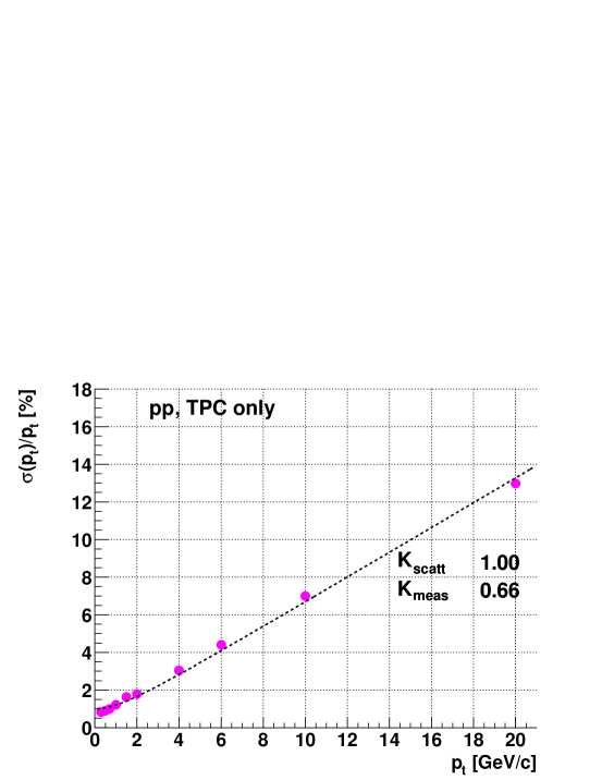
Figure 4.8: Relative $p_{\rm t}$ resolution in the TPC for pp events with $B=0.4$ T. The resolution is fitted to the expression $\sigma(p_{\rm t})/p_{\rm t}=K_{\rm scatt}\oplus K_{\rm meas}\cdot p_{\rm t}$.

In the TPC the spatial resolution of the space points can be assumed as constant only in the case of pp collisions; in fact, in the high-multiplicity environment of heavy ion collisions, the clusters overlap in the inner part of the detector and the resolution is worse than in the outer part. The fit of the relative $p_{\rm t}$ resolution, in pp collisions, in the TPC (see Fig. 4.8) to the expression (4.1) gives:

$$\frac{\sigma(p_{\rm t})}{p_{\rm t}}\simeq 1.00\%\oplus 0.66\%\cdot p_{\rm t}(\mathrm{GeV}/c).$$ (4.3)

The obtained value for $K_{\rm meas}$ is in good agreement with the value 0.65%, calculated using $\sigma_{r\phi}=0.8\leavevmode\nobreak\ \mathrm{mm}$ [83], $N=100$ [84], $\ell=1.6\leavevmode\nobreak\ \mathrm{m}$ and $B=0.4$ T.

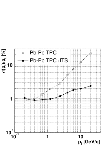
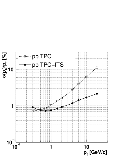
Figure 4.9: Relative $p_{\rm t}$ resolution in the TPC and in TPC–ITS, for Pb–Pb (left) and for pp events (right). The value of the magnetic field is $B=0.4$ T.

The relative transverse momentum resolution, as a function of the transverse momentum, is shown in Fig. 4.9. The resolutions achieved in the TPC and in TPC–ITS are compared on the same plot, for Pb–Pb (left panel) and for pp events (right panel). For the definition of the resolution, the reconstructed $p_{\rm t}$ is compared to the ‘true’ $p_{\rm t}$ at the entrance of the TPC, for the TPC, and to the ‘true’ $p_{\rm t}$ at the interaction point, for TPC–ITS. This is the reason why the resolution at very low $p_{\rm t}$ is better for the TPC alone: at low $p_{\rm t}$ the resolution is dominated by multiple scattering, which is much lower in the TPC gas than in the layers of the ITS. But the most striking feature is the improvement of about one order of magnitude for high-$p_{\rm t}$ tracks when including the ITS. This effect is partially due to the increased lever arm ($\ell_{\rm TPC}\simeq 1.6\leavevmode\nobreak\ \mathrm{m}$ in the TPC and $\ell_{\rm TPC-ITS}\simeq 2.5\leavevmode\nobreak\ \mathrm{m}$ in TPC–ITS), which accounts for an improvement of a factor $(\ell_{\rm TPC-ITS}/\ell_{\rm TPC})^{2}\simeq 2.5$. The remaining difference is due to the much better spatial resolution of the points in the ITS, with respect to those in the TPC. For TPC–ITS the $p_{\rm t}$ resolution in pp is $\approx 15$-$20\%$ better than in Pb–Pb.

Parameterization of TPC tracking response: a tool for high-statistics simulation studies

The computing time and disk space requirements for the detailed simulation of the TPC are very large and they correspond to more than 90% of the total requirements for the tracking dedicated detectors of the ALICE barrel (ITS and TPC). The size of the file containing the hits and the digits (in addition to the kinematic information on the generated particles) for 1 central Pb–Pb event produced with HIJING is $0.02$ Gbytes if only the ITS is included and 1.2 Gbytes if also the detailed description of the TPC is included. Similar proportions are maintained also for pp events. This implies that the complete simulation of the TPC cannot be used in the studies of physics signals requiring a large number of events. The study for the detection of open charm via hadronic decays is a typical example. In fact, as we will see in Chapter 6, the selection strategy to extract the D meson signal out of the large combinatorial background has to be optimized on a very large sample of events ($\sim 10^{4}$-$10^{5}$ for Pb–Pb and $\sim 10^{6}$-$10^{7}$ for pp). The required statistics is similar also for the studies on semi-electronic charm and beauty decays and on hyperon decays ($\Xi$ and $\Omega$, in particular). In all these cases, the performance of the apparatus is determined mainly by the ITS, which is dedicated to the reconstruction of secondary vertices. Therefore, the optimal solution is to use a detailed simulation of the ITS (and of the beam pipe material) and a parameterization of the response of the tracking algorithm in the TPC.

The design and implementation of this parameterization, developed specifically in the scope of this thesis work, is described in an ALICE Internal Note [85]. We remark that this work allowed also a systematic study of the response of TPC tracking and a fruitful analysis of the error handling in the tracking algorithm (see Ref. [85] for details).

In the following we outline the idea on which the tool is based. The tests that were performed in order to validate the tool for the use in physics studies are reported in Appendix C.

After the Kalman filter reconstruction in the TPC, the tracks that have been found are described by the state vector and its covariance matrix, defined at a reference plane corresponding to the radial position of the inner pad row of the TPC. At this stage all the information from the TPC is ‘summarized’ in the state vector and the covariance matrix. Such tracks are taken as seeds for the track finding algorithm in the ITS.

The idea is to parameterize the response of the TPC at this level and create the TPC reconstructed tracks taking as a starting point the generated tracks. Since for every track entering the TPC in a sensitive region the position and the momentum in the entering point are stored (hit), it is possible to determine the exact state vector of the track at the reference plane. Then, the following steps are performed:

1. Apply a first selection based on the geometrical acceptance of the TPC.

2. Assign a covariance matrix to the track. This is done using look-up tables.

3. Smear the track parameters according to the Kalman filter resolutions, by means of the covariance matrix.

4. Assign a value of d$E/$d$x$ to the track. This is important because the d$E/$d$x$ from the TPC is used to make a mass hypothesis for the estimation of multiple scattering and energy loss during tracking in the ITS.

5. Apply a second selection based on the efficiency of the TPC (which accounts for decays, detector and tracking algorithm efficiency).

In all these steps different track kinematics and particle types are appropriately taken into account. The tracks ‘built’ with this procedure can be used to seed the standard reconstruction with the Kalman filter in the ITS. Since only the information at the inner radius of the TPC is required, the transport done by GEANT can be stopped at $r\simeq 90$ cm and the digitization of the TPC is not needed. This reduces the simulation requirements in terms of disk space and computing time by a factor $\simeq 35$. Is was verified that the performance of the ITS tracking, in terms of tracking efficiency and resolutions on the track parameters, is not altered by the use of this parameterized tracking in the TPC (see Appendix C). The parameterization was realized for Pb–Pb events with ${\rm d}N_{\rm ch}/{\rm d}y=6000$ and for pp events, at $B=0.4\leavevmode\nobreak\$T.

4.3 LHC beams and interaction region

The running strategy for the heavy ion program at the LHC, along with the dependence on the colliding system of the available energy in the centre of mass were discussed in Section 1.4.1. Here we focus on the features of the particle beams at the ALICE intersection point (IP) and, consequently, of the interaction region, the region in space that contains all the possible collision vertices. These parameters are, indeed, very important for the reconstruction of secondary vertices, as we will see in the next chapters.

In Section 4.3.1 we will define the luminosity and show how it is related to the size of the interaction region. Then, we will consider the specific cases of Pb–Pb (Section 4.3.2) and pp (Section 4.3.3) running.

4.3.1 Luminosity and beam size

The event rate $R$ in a collider is proportional to the interaction cross section $\sigma_{\rm int}$ and the factor of proportionality is called luminosity (${\cal L}$):

$$R={\cal L}\,\sigma_{\rm int}.$$ (4.4)

The luminosity, as we will show, is entirely defined by the characteristics of the colliding beams at the interaction point, and it is an important issue, because there are limitations on the maximum event rate coming from both the ALICE detector and the accelerator. As we will detail in the next sections, in the case of Pb–Pb events the limitations of the detector and of the machine coincide, while in the case of pp events the maximum event rate is determined by the detector and the machine parameters have to be tuned in order not to exceed this limit.

Let us consider two intersecting bunches, labelled 1 and 2. To a good approximation, the particles in each of them will be distributed according to Gaussians in the three perpendicular directions [60]:

$$N_{i}(x,y,z)=N_{i}\,G(x,\overline{x}_{i},\sigma_{x,i})\,G(y,\overline{y}_{i},\sigma_{y,i})\,G(z,\overline{z}_{i},\sigma_{z,i})\leavevmode\nobreak\ \leavevmode\nobreak\ \leavevmode\nobreak\ \leavevmode\nobreak\ \leavevmode\nobreak\ \leavevmode\nobreak\ \leavevmode\nobreak\ \leavevmode\nobreak\ i=1,\leavevmode\nobreak\ 2$$ (4.5)

where $N_{i}$ is the total number of particles in the bunch $i$ and

$$G(q,\overline{q},\sigma_{q})=\frac{1}{\sqrt{2\pi}\sigma_{q}}\exp\left[-\frac{(q-\overline{q})^{2}}{2\sigma_{q}^{2}}\right]\leavevmode\nobreak\ \leavevmode\nobreak\ \leavevmode\nobreak\ \leavevmode\nobreak\ \leavevmode\nobreak\ \leavevmode\nobreak\ \leavevmode\nobreak\ \leavevmode\nobreak\ \leavevmode\nobreak\ \leavevmode\nobreak\ \leavevmode\nobreak\ \leavevmode\nobreak\ \leavevmode\nobreak\ \leavevmode\nobreak\ \leavevmode\nobreak\ \leavevmode\nobreak\ \leavevmode\nobreak\ q=x,\leavevmode\nobreak\ y,\leavevmode\nobreak\ z.$$ (4.6)

If $f$ is the revolution frequency and $N_{\rm b}$ is the number of bunches, the luminosity is obtained as:

$${\cal L}=f\,N_{\rm b}\times\int{\rm d}x\,{\rm d}y\,{\rm d}z\,N_{1}(x,y,z)\,N_{2}(x,y,z).$$ (4.7)

Here, the integration along the beam direction, $z$, gives 1, since the two particle bunches cross each other and, therefore, their distributions along $z$ are equivalent to delta functions from the point of view of the interaction probability.

At the LHC the bunches in the two beams have the same number of particles ($N$) and the same dispersions; moreover the dispersion is the same for the two directions transverse to the beam axis ($\sigma_{x}=\sigma_{y}=\sigma_{x,y}$). Thus:

$${\cal L}=f\,N_{\rm b}\,\frac{N^{2}}{4\pi\sigma_{x,y}^{2}}\exp\left[-\frac{d^{2}}{4\sigma_{x,y}^{2}}\right]$$ (4.8)

where $d^{2}=(\Delta\overline{x})^{2}+(\Delta\overline{y})^{2}$ is the square of the distance between the centres of the two beams. Normally, the two beams are centred and $d=0$.

On the other hand, the interaction region is defined as the convolution of the two particle distributions in the two intersecting bunches: the interaction vertex lies in a ‘diamond’ with ‘dimensions’

$$\sigma^{\rm vertex}_{q}=\sigma_{q}/\sqrt{2}\leavevmode\nobreak\ \leavevmode\nobreak\ \leavevmode\nobreak\ \leavevmode\nobreak\ \leavevmode\nobreak\ \leavevmode\nobreak\ \leavevmode\nobreak\ \leavevmode\nobreak\ \leavevmode\nobreak\ q=x,\leavevmode\nobreak\ y,\leavevmode\nobreak\ z$$ (4.9)

that do not depend on the value of $d$, if the distributions are gaussian.

The size of the bunches at the IP depends on the transverse emittance $\epsilon$ (a beam quality parameter) and on the value of the amplitude function $\beta$ at the IP, indicated as $\beta^{\star}$, which is determined by the accelerator magnets configuration. We have [60]:

$$\sigma_{q}=\sqrt{\frac{\epsilon_{q}\,\beta^{\star}}{\pi}}\leavevmode\nobreak\ \leavevmode\nobreak\ \leavevmode\nobreak\ \leavevmode\nobreak\ \leavevmode\nobreak\ \leavevmode\nobreak\ \leavevmode\nobreak\ \leavevmode\nobreak\ \leavevmode\nobreak\ \leavevmode\nobreak\ q=x,\leavevmode\nobreak\ y,\leavevmode\nobreak\ z.$$ (4.10)

From the last three equations we see that the luminosity can be decreased locally (i.e. only at the ALICE IP) by increasing $\beta^{\star}$, but this increases the transverse size of the interaction region. In Table 4.3 we report the LHC machine nominal parameters at the ALICE IP for pp and Pb–Pb runs [24]. We will discuss them in the next sections.

Table 4.3: LHC parameters for pp and Pb–Pb runs at the ALICE IP [24].

Parameter		pp	Pb–Pb
Energy per nucleon	[TeV]	7	2.76
$\beta^{\star}$	[m]	10	0.5
$\sigma_{x,y}$	$[\mathrm{\mu m}]$	71	16
$\sigma_{z}$	$[\mathrm{cm}]$	7.5	7.5
$\sigma^{\rm vertex}_{x,y}$	$[\mathrm{\mu m}]$	50	11
$\sigma^{\rm vertex}_{z}$	$[\mathrm{cm}]$	5.3	5.3
Luminosity	$[\mathrm{cm}^{-2}\mathrm{s}^{-1}]$	$5\times 10^{32}$	$10^{27}$

4.3.2 Interaction region in Pb–Pb collisions

When taking data with Pb–Pb beams the ALICE detector is limited to a maximum luminosity of $10^{27}\leavevmode\nobreak\ \mathrm{cm}^{-2}\mathrm{s}^{-1}$ by the drift time in the Time Projection Chamber. Due to the maximum allowed heating in the beam pipe it is currently assumed that the maximum Pb–Pb luminosity at the LHC is also limited to $0.5$-$1\times 10^{27}\leavevmode\nobreak\ \mathrm{cm}^{-2}\mathrm{s}^{-1}$.

The parameters of the Pb beams ($N,\leavevmode\nobreak\ N_{\rm b},\leavevmode\nobreak\ f$) are, therefore, tuned in order to have $\mathcal{L}\simeq 10^{27}\leavevmode\nobreak\ \mathrm{cm}^{-2}\mathrm{s}^{-1}$ while running with a low value of $\beta^{\star}$ ($0.5\leavevmode\nobreak\ \mathrm{m}$), which allows to focus very well the beams in the transverse plane. The transverse size of the beams at the ALICE IP is $\sigma_{x,y}\simeq 16\leavevmode\nobreak\ \mathrm{\mu m}$ and the transverse size of the interaction region is $\sigma_{x,y}/\sqrt{2}\simeq 11\leavevmode\nobreak\ \mathrm{\mu m}$. Since the position of the centres of the beams is stable for a given run (of a duration of about 4 hours), the mean position of the interaction point during each run is measured with very high precision, by integration over a long time interval. Therefore, the uncertainty on the vertex position in the transverse plane can be assumed to be given by the size of the interaction region: $\sigma_{\rm vertex}\simeq 11\leavevmode\nobreak\ \mathrm{\mu m}$.

Along the $z$ direction, the interaction point is distributed according to a Gaussian with a dispersion of $\simeq 5.3\leavevmode\nobreak\ \mathrm{cm}$ and the ALICE interaction trigger selects the events with vertex located in the fiducial region $-5.3<z<5.3\leavevmode\nobreak\ \mathrm{cm}$. Clearly, the position of the vertex in $z$ has to be reconstructed on an event-by-event basis. This task is achieved exploiting the correlation between clusters in the two silicon pixel layers of the ITS [86, 87]; the results of this method will be briefly described in Chapter 5.

4.3.3 Interaction region in pp collisions

For the pp runs ALICE will take data in parallel with the pp-dedicated experiments, which will exploit the maximum design luminosity of the LHC for pp, ${\cal L}\simeq 10^{34}\leavevmode\nobreak\ \mathrm{cm}^{-2}\leavevmode\nobreak\ \mathrm{s}^{-1}$. The nominal luminosity at the ALICE IP, reduced using a larger value of $\beta^{\star}$ with respect to the other experiments, is $5\times 10^{32}\leavevmode\nobreak\ \mathrm{cm}^{-2}\mathrm{s}^{-1}$. Nevertheless, this nominal luminosity has to be reduced to $<3\times 10^{30}\leavevmode\nobreak\ \mathrm{cm}^{-2}\mathrm{s}^{-1}$, in order to limit the pile-up of events in the TPC and in the Silicon Drift Detectors (SDD).

As we can see from Eq. (4.8), such reduction can be achieved in two ways:

• by further increasing the value of $\beta^{\star}$ and/or

• by displacing the two beams in the transverse plane ($d>0$) to make a collision between the tails of the particle distributions.

If the first option is chosen, $\beta^{\star}$ might be increased up to $100\leavevmode\nobreak\ \mathrm{m}$; this would broaden of a factor $\sqrt{100\leavevmode\nobreak\ \mathrm{m}/10\leavevmode\nobreak\ \mathrm{m}}\simeq 3$ the transverse size of the interaction ‘diamond’, with respect to the nominal value reported in Table 4.3, up to $\simeq 150\leavevmode\nobreak\ \mathrm{\mu m}$.

If the second option is necessary, the beams might be displaced to a distance of $\simeq 4$-$5\leavevmode\nobreak\ \sigma_{x,y}\simeq 300\leavevmode\nobreak\ \mathrm{\mu m}$ and the collisions will occur in the tails at $4$-$5\leavevmode\nobreak\ \sigma$ from the centre of the beams: these tails will much likely be non-gaussian and the size of the interaction ‘diamond’ may be even larger than $150\leavevmode\nobreak\ \mathrm{\mu m}$.

For what concerns the $z$ direction, the situation will be the same as for the heavy ion running.

Given that the uncertainty on the vertex position in the transverse plane might be even larger than the mean decay length of neutral charm mesons ($c\tau\simeq 123\leavevmode\nobreak\ \mathrm{\mu m}$), we conclude that the position of the interaction vertex in pp collisions has to be reconstructed in all three dimensions, and not only along $z$ as in Pb–Pb, on an event-by-event basis. A large part of the next chapter is dedicated to this topic. In Chapter 6 we demonstrate that the uncertainty on the position of the interaction vertex is the main limiting factor for the performance of ALICE in the exclusive reconstruction of charm particles in proton–proton events.

Chapter 5 Identification of heavy flavour decay vertices: experimental issues

Secondary vertices are the signature of the (weak) decay of particles containing strangeness, charm or beauty. The identification of these decays is particularly challenging in the case of open charm and open beauty hadrons that have mean proper decay lengths of $\sim 100$-$500\leavevmode\nobreak\ \mathrm{\mu m}$, namely D⁰ ($c\tau\simeq\leavevmode\nobreak\ 123\leavevmode\nobreak\ \mathrm{\mu m}$), D⁺ ($c\tau\simeq\leavevmode\nobreak\ 315\leavevmode\nobreak\ \mathrm{\mu m}$) and B mesons ($c\tau\sim\leavevmode\nobreak\ 500\leavevmode\nobreak\ \mathrm{\mu m}$) [60].

The most effective constraint for the selection of such particles is the presence of one or more tracks that are displaced from the interaction (primary) vertex. The variable allowing to evaluate the displacement of a track is its impact parameter, which was defined in Chapter 2 as the distance of closest approach of the reconstructed particle trajectory to the primary vertex.

Now that the procedure for track reconstruction in the ALICE barrel has been described (Section 4.2.3), a more precise definition of the two projections of the impact parameter, in the transverse plane and along the beam direction, can be given. After the reconstruction, the state vector of the track is given at the radial position corresponding to the inner pixel layer ($r\simeq 4\leavevmode\nobreak\ \mathrm{cm}$), where the last cluster assigned to the track lies. From this point the state vector is propagated to the radius of the beam pipe ($r\simeq 3\leavevmode\nobreak\ \mathrm{cm}$) and a correction is applied to the track curvature in order to account for the energy loss in the material ($0.8\leavevmode\nobreak\ \mathrm{mm}$ of beryllium). The impact parameter projection in the transverse (bending) plane, $d_{0}(r\phi)$, is defined as:

$$d_{0}(r\phi)\equiv q\cdot\left[R-\sqrt{(x_{V}-x_{C})^{2}+(y_{V}-y_{C})^{2}}\right],$$ (5.1)

where $q$ is the sign of the particle charge, $R$ and $(x_{C},y_{C})$ are the radius and the centre of the track projection in the transverse plane (which is a circle) and $(x_{V},y_{V})$ is the position of the primary vertex in the transverse plane. In this way, the impact parameter has also a sign; this is very useful for the identification of specific topologies, in particular for the $\mbox{$\mathrm{D^{0}}$}\to\mbox{$\mathrm{K}$}^{-}\pi^{+}$ decay, as we will see in the next chapter. The $z$ projection of the impact parameter, $d_{0}(z)$, is defined as:

$$d_{0}(z)\equiv z_{\rm track}-z_{V},$$ (5.2)

where $z_{\rm track}$ is the $z$ position of the track after it has been propagated to the distance of closest approach in the bending plane, and $z_{V}$ is the position of the primary vertex along the beam direction.

Clearly, for both the $r\phi$ and $z$ projections, the impact parameter resolution has a contribution due to the track position resolution and a contribution due to the uncertainty on the primary vertex position:

$$\sigma(d_{0})=\sigma_{\rm track}\oplus\sigma_{\rm vertex}.$$ (5.3)

Since the $r\phi$ impact parameter of the decay products of $\mathrm{D^{0}}$ mesons is of the order of $100\leavevmode\nobreak\ \mathrm{\mu m}$, as shown in Appendix A, it is crucial to achieve a very good resolution ($<50$-$60\leavevmode\nobreak\ \mathrm{\mu m}$) not only on the track position at the vertex, but also on the position in $r\phi$ of the primary vertex itself.  

We consider separately the two cases of Pb–Pb (or, more generally, heavy ion) events and pp events.

We have seen in Section 4.3 that, in the former case, the transverse beam size is very small and the primary vertex position is know for a given run with an uncertainty of only $\simeq 10\leavevmode\nobreak\ \mathrm{\mu m}$. This uncertainty is negligible and, therefore, the resolution on $d_{0}(r\phi)$ coincides with the resolution on the track position. In Section 5.1 we show how the pixel detector provides, before track reconstruction, a very precise estimate of the position along $z$ of the interaction point. Then, we report on the performance of ALICE for the measurement of the track impact parameter in heavy ion collisions (Section 5.2). The achieved resolution is studied as a function of particle kinematics and particle type, and the effect of missing or misassigned clusters in the ITS is discussed.

In the case of pp running, since the beams have to be defocused and/or displaced to reduce the luminosity, the a priori information on the vertex position might be extremely poor ($\sigma\sim 150\leavevmode\nobreak\ \mathrm{\mu m}$) and an event-by-event reconstruction of all the three coordinates is mandatory in order to fulfill the resolution requirements stated above. A method to accomplish this task is presented in Section 5.3. The achieved resolution on the the vertex is eventually combined with that on the track position to obtain the impact parameter resolution in pp events (Section 5.4).

Finally, we describe the reconstruction of the secondary vertex position in the case of the two-body decay $\mbox{$\mathrm{D^{0}}$}\to\mbox{$\mathrm{K}$}^{-}\pi^{+}$ (Section 5.5). We show the achieved spatial resolution, which is important for the precise determination of the $\mathrm{D^{0}}$ flight line and, consequently, of the pointing angle, the other key variable for the identification of displaced vertex topologies.

5.1 Primary vertex reconstruction in Pb–Pb

Along the $z$ direction, the interaction points are distributed according to a Gaussian with $\sigma=5.3\leavevmode\nobreak\ \mathrm{cm}$, both in heavy ion and in pp runs (Section 4.3). The $z$ coordinate of the primary vertex in heavy ion collisions can be measured very precisely, before track reconstruction, using the correlation between clusters in the two pixel layers at $r=4\leavevmode\nobreak\ \mathrm{cm}$ and $r=7\leavevmode\nobreak\ \mathrm{cm}$ [86, 87]. A tracklet (line segment), built from two clusters generated by the same track, points to the primary vertex and gives an estimate of its position along $z$. All pairs of clusters in the two layers are considered and the background from uncorrelated pairs is partially removed requiring the two clusters to lie within the same (small) azimuthal window $\Delta\phi$. The achieved resolution on $z_{V}$ is proportional to $1/\sqrt{N_{\rm tracklets}}$, where $N_{\rm tracklets}$ is the number of tracklets from correlated clusters, which is proportional to the event multiplicity ${\rm d}N_{\rm ch}/{\rm d}y$. The resolution in heavy ion collisions was parameterized as [86]:

$$\sigma_{z}({\rm d}N_{\rm ch}/{\rm d}y)=\left(2+\frac{292}{\sqrt{{\rm d}N_{\rm ch}/{\rm d}y}}\right)\leavevmode\nobreak\ \mathrm{\mu m},$$ (5.4)

where the constant additive term is due to the residual background of uncorrelated clusters. The resolution is $\simeq 5\leavevmode\nobreak\ \mathrm{\mu m}$ for ${\rm d}N_{\rm ch}/{\rm d}y=6000$ and $\simeq 7\leavevmode\nobreak\ \mathrm{\mu m}$ for a lower multiplicity, ${\rm d}N_{\rm ch}/{\rm d}y=3000$. Therefore, in Pb–Pb also the uncertainty on $z_{V}$ is negligible and the resolution on the $z$ projection of the impact parameter is given only by the track position resolution.

We adapted and tuned this method for the estimate of $z_{V}$ also in pp collisions [88]. The resolution was studied as a function of the multiplicity in pp events simulated with PYTHIA. The result is [88]:

$$\sigma_{z}({\rm d}N_{\rm ch}/{\rm d}y)=\left(42+\frac{290}{\sqrt{{\rm d}N_{\rm ch}/{\rm d}y}}\right)\leavevmode\nobreak\ \mathrm{\mu m}.$$ (5.5)

The value corresponding to the average multiplicity predicted by PYTHIA for pp non-diffractive events at $\sqrt{s}=14\leavevmode\nobreak\ \mathrm{TeV}$ (${\rm d}N_{\rm ch}/{\rm d}y=6$) is $\simeq 160\leavevmode\nobreak\ \mathrm{\mu m}$. Although not very precise, it is important to have an estimate of the vertex position along $z$ before track reconstruction; this information is, indeed, helpful to improve the track finding efficiency in the ITS.

5.2 Track impact parameter resolution in Pb–Pb

5.2.1 Transverse momentum dependence

For the estimation of the $d_{0}$ $r\phi$- and $z$-resolution as a function of the transverse momentum, we superimposed samples of 500 particles, 50% positively charged and 50% negatively charged, with a given $p_{\rm t}$ and homogeneously distributed in $|\eta|<0.9$, on top of standard Pb–Pb central events, with collision impact parameter $b<2\leavevmode\nobreak\ \mathrm{fm}$, generated with HIJING. For each considered $p_{\rm t}$ value 10 such combined events were used. The magnetic field was set to 0.4 T. In the ITS the clusters were obtained using a realistic simulation of the detector response (slow points) and track reconstruction in TPC–ITS was performed as described in Chapter 4.

At first we consider primary charged pions reconstructed in the TPC and in the ITS, with a cluster in each ITS layer; this is very important, because the impact parameter resolution is strongly dependent on the number of clusters associated to the track in the ITS, and, in particular, on the presence of the clusters in the two pixel layers, as we shall detail in the following.

The resolutions, obtained from a gaussian fit to the $d_{0}$ distributions, are presented in Fig. 5.1 as a function of the track transverse momentum. The resolution in $r\phi$ ($z$) is $65\leavevmode\nobreak\ (170)\leavevmode\nobreak\ \mathrm{\mu m}$ at $p_{\rm t}=1\leavevmode\nobreak\ \mathrm{GeV}/c$ and $12\leavevmode\nobreak\ (40)\leavevmode\nobreak\ \mathrm{\mu m}$ at $p_{\rm t}=20\leavevmode\nobreak\ \mathrm{GeV}/c$. The large difference between the two projections reflects the different spatial resolutions in the $r\phi$ and $z$ directions of the detectors in the ITS (see Table 4.1). A more detailed analysis of the $p_{\rm t}$-dependence of the resolutions and of their value at high $p_{\rm t}$ can be found in Appendix D, along with a study of their dependence on the thickness of the two pixel layers.

A resolution on $d_{0}(r\phi)$ better than $65\leavevmode\nobreak\ \mathrm{\mu m}$ ($\approx c\tau(\mbox{$\mathrm{D^{0}}$})/2$) for $p_{\rm t}>1\leavevmode\nobreak\ \mathrm{GeV}/c$ is, in principle, sufficient to separate from the background the tracks from a $\mathrm{D^{0}}$ decay and, therefore, the Inner Tracking System with pixel detectors fulfills its most severe design requirement.

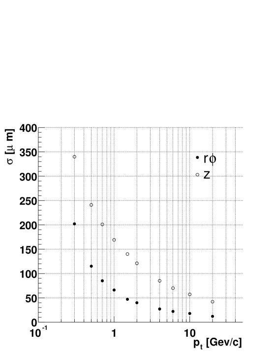
Figure 5.1: Impact parameter resolutions for primary charged pions reconstructed in the TPC and in the ITS (with 6 clusters in the ITS) in central Pb–Pb collisions (${\rm d}N_{\rm ch}/{\rm d}y=6000$).

5.2.2 Effect of missing and misassigned clusters

We now consider the effect on the impact parameter resolution of misassigned or missing clusters in the ITS layers. We focus on the $r\phi$ impact parameter for pions with $p_{\rm t}\approx 1\leavevmode\nobreak\ \mathrm{GeV}/c$. Figure 5.3 (left) shows that the distribution of the impact parameters for fake tracks (at least 1 misassigned cluster) is much broader than that for tracks with 6 correctly-assigned clusters. However, since the fraction of fake tracks is $\simeq 5\%$ at $p_{\rm t}=1\leavevmode\nobreak\ \mathrm{GeV}/c$ and it vanishes very rapidly as $p_{\rm t}$ increases (as shown in Section 4.2.3—Fig. 4.7), for relatively large $p_{\rm t}$ tracks, the effect due to misassigned clusters is very small, if 6 ITS clusters are required.

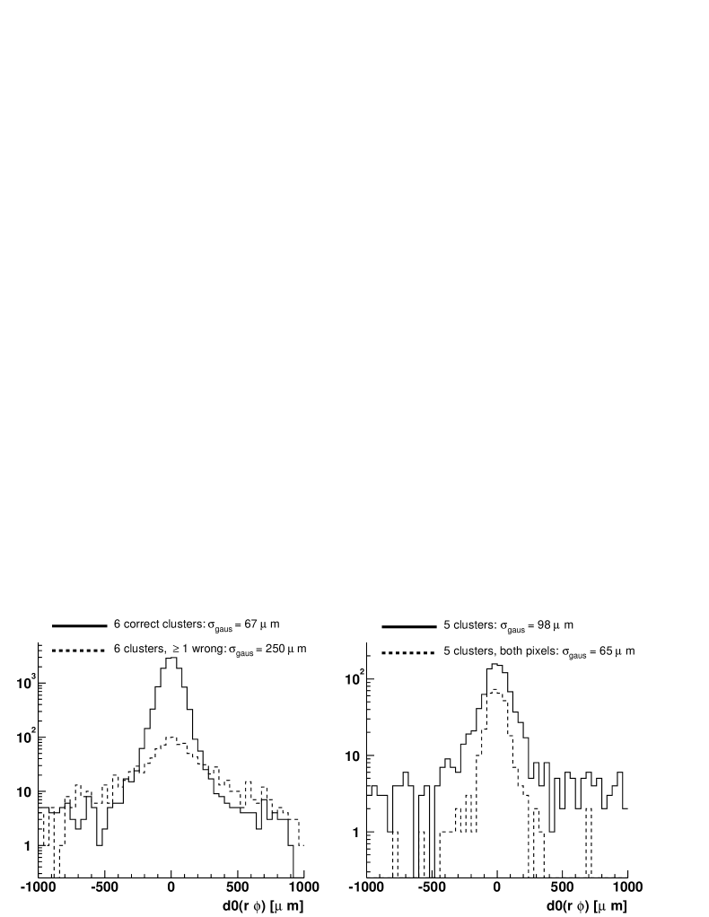
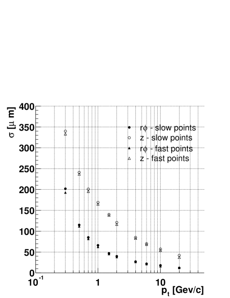
Figure 5.2: Distributions of the $r\phi$ impact parameter for primary pions with $p_{\rm t}\approx 1\leavevmode\nobreak\ \mathrm{GeV}/c$. On the left, tracks with 6 correctly assigned ITS clusters (solid) and fake tracks, with at least 1 misassigned cluster (dashed). On the right, tracks with 5 ITS clusters (solid) and tracks with 5 clusters but with clusters in the pixel layers (dashed). We report the resolutions estimated with a gaussian fit.

Figure 5.3: Comparison of the resolutions obtained with detailed (circles) and with fast (triangles) response of the ITS.

As it can be seen in Fig. 5.3 (right), for tracks with only 5 clusters in the ITS, the resolution is still good if there is a cluster in each of the pixel layers. Therefore, for the physics studies requiring an optimal impact parameter resolution, the loosest track quality condition is to have at least 5 clusters in the ITS and two of these in the pixel layers. This increases the total number of ‘tracks for physics’ by 8%, with respect to requiring always all 6 points in the ITS; the increase is 5% for $p_{\rm t}>0.5\leavevmode\nobreak\ \mathrm{GeV}/c$ and 4% for $p_{\rm t}>0.8\leavevmode\nobreak\ \mathrm{GeV}/c$.

5.2.3 Comparison of detailed and fast ITS simulation

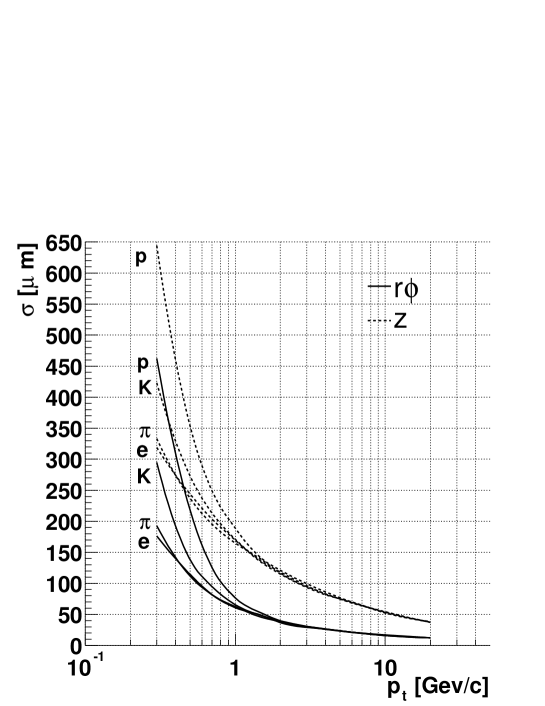
Figure 5.4: Impact parameter resolutions for electrons, pions, kaons and protons as a function of the transverse momentum.

Physics simulation studies requiring very large statistics (e.g. open charm and open beauty feasibility studies) use a simplified and faster version of the detector response of the the ITS (fast points). In this fast simulation approach the position of the clusters in each layer is directly obtained from the position of the hits (the points where the particles crossed the sensitive volume) applying a gaussian smearing in $r\phi$ and in $z$ that accounts for the detector spatial precision (the precisions used for the 6 layers are those reported in Table 4.1). It is, therefore, very important to observe, see Fig. 5.3, that the impact parameter resolution is essentially not altered by the use of the fast response of the ITS.

5.2.4 Particle type dependence

For low momenta, the main contribution to the impact parameter resolution is due to the multiple scattering, which depends on $1/\beta$ [60]. Consequently, for a given $p_{\rm t}$, the resolution itself is worse for heavier particles, that have lower velocity $\beta$. Figure 5.4 presents the resolutions for electrons ($e^{\pm}$), pions ($\pi^{\pm}$), kaons ($\rm K^{\pm}$) and protons ($\rm p$ and $\rm\overline{p}$). For $p_{\rm t}>1\leavevmode\nobreak\ (1.5)\leavevmode\nobreak\ \mathrm{GeV}/c$ the resolutions for kaons (protons) are the same as for pions.

The separation at low $p_{\rm t}$ between pions and electrons is not well defined, because the latter can suffer from energy loss due to the bremsstrahlung process; even if the probability is quite low ($\sim 1\%$ at $p_{\rm t}=1\leavevmode\nobreak\ \mathrm{GeV}/c$), this spoils both the momentum and the impact parameter resolution.

5.3 Primary vertex reconstruction in pp

5.3.1 Outline of the method

After track reconstruction in TPC and ITS, all tracks are propagated to the nominal position of the interaction vertex, which, during the proton–proton running, will be given by the machine with a resolution of $\sim 100$-$200\leavevmode\nobreak\ \mathrm{\mu m}$ (Section 4.3.3).

The reconstruction in three dimensions of the primary vertex position by means of the reconstructed tracks is performed in two steps:

1. Vertex finding: a first estimate of the vertex position is obtained using track pairs.

2. Vertex fitting: tracks are propagated to the position estimated in the first step and the optimal estimate of the vertex position, as well as the vertex covariance matrix and a ‘quality parameter’ ($\chi^{2}$), are obtained via a fast fitting algorithm. In this step a cut on the maximum contribution to the total $\chi^{2}$ is applied in order to remove secondary tracks from the fit.

The algorithm was tested on a sample of 5000 minimum-bias pp events at $\sqrt{s}=14\leavevmode\nobreak\ \mathrm{TeV}$ (without single- and double-diffractive topologies) generated with PYTHIA, as described in Section 4.2.1. The generated vertex position was sampled along $z$ from a Gaussian centred at $z=0$ with $\sigma_{z}=5.3\leavevmode\nobreak\ \mathrm{cm}$. The sampling was limited in the region $-\sigma_{z}<z<+\sigma_{z}$. The coordinates in the bending plane were sampled from 2 Gaussians with dispersions $\sigma_{x}=\sigma_{y}=150\leavevmode\nobreak\ \mathrm{\mu m}$. In order to simulate a beam-offset condition, the two Gaussians were centred at $x_{0}=y_{0}=5\leavevmode\nobreak\ \mathrm{mm}$.

5.3.2 Expected resolutions

The attainable resolution on the vertex position can be estimated on the basis of the resolutions on the track position in the bending plane and in the longitudinal direction, which are shown in Fig. 5.1.

The average number of reconstructed tracks in pp non-diffractive events is $\left\langle N\right\rangle\simeq 7$ and the average value of the transverse momentum for these tracks is $\left\langle p_{\rm t}\right\rangle\simeq 0.6\leavevmode\nobreak\ \mathrm{GeV}/c$. Therefore, the expected resolutions on the $x$ (for $y$ it is the same) and on the $z$ coordinate of the vertex are:

$$\begin{array}[]{l}\sigma_{\rm vertex}(x)=\sigma_{\rm track}(r\phi)_{p_{\rm t}=0.6\leavevmode\nobreak\ \mathrm{GeV}/c}\bigg{/}\sqrt{\left\langle N\right\rangle/2}\simeq 110\leavevmode\nobreak\ \mathrm{\mu m}\bigg{/}\sqrt{3.5}=60\leavevmode\nobreak\ \mathrm{\mu m}\\ \sigma_{\rm vertex}(z)=\sigma_{\rm track}(z)_{p_{\rm t}=0.6\leavevmode\nobreak\ \mathrm{GeV}/c}\bigg{/}\sqrt{\left\langle N\right\rangle}\simeq 240\leavevmode\nobreak\ \mathrm{\mu m}\bigg{/}\sqrt{7}=90\leavevmode\nobreak\ \mathrm{\mu m}.\end{array}$$ (5.6)

For the $x$ (and $y$) coordinate the number of contributing tracks is taken equal to $\left\langle N\right\rangle/2$, since, in the transverse plane, the information from $\left\langle N\right\rangle$ tracks is used to determine 2 coordinates.

5.3.3 Vertex finding

The reconstructed tracks are propagated to the radial position corresponding to the nominal vertex position in the bending plane. Such position is expected to be known with a precision of the order of $100$-$200\leavevmode\nobreak\ \mathrm{\mu m}$, however the vertex finding procedure should succeed even though the nominal position is known with a poorer accuracy. The nominal position used in the test is $(x_{\rm nom}=0,y_{\rm nom}=0)$, i.e. $\approx 7\leavevmode\nobreak\ \mathrm{mm}$ far from the generated position, in order to check the performance of the vertex recognition algorithm in a condition far worse than expected.

A loose cut ($3\leavevmode\nobreak\ \mathrm{cm}$) on the transverse impact parameter of the tracks is applied in order to exclude particles originating from secondary vertices well displaced with respect to the primary vertex.

Each track is approximated with the straight line tangent to the reconstructed helix at the nominal vertex position. Then, all possible track pairs $(i,j)$ are considered and, for each pair, the centre $C(i,j)\equiv(x_{ij},y_{ij},z_{ij})$ of the segment of minimum approach between the two lines is found. The coordinates of the primary vertex are determined as:

$$q_{\rm found}={1\over N_{\rm pairs}}\sum_{i,j}q_{ij}\leavevmode\nobreak\ \leavevmode\nobreak\ \leavevmode\nobreak\ \leavevmode\nobreak\ \leavevmode\nobreak\ \leavevmode\nobreak\ \leavevmode\nobreak\ \leavevmode\nobreak\ \leavevmode\nobreak\ \leavevmode\nobreak\ \leavevmode\nobreak\ \leavevmode\nobreak\ \leavevmode\nobreak\ \leavevmode\nobreak\ \leavevmode\nobreak\ \leavevmode\nobreak\ q=x,\leavevmode\nobreak\ y,\leavevmode\nobreak\ z$$ (5.7)

where $N_{\rm pairs}$ is the number of track pairs.

The obtained resolution on the position of the vertex is of order $100\leavevmode\nobreak\ \mathrm{\mu m}$ for all three coordinates [88]. The results are actually independent of the value used for the nominal position of the primary vertex, when this is in the range of few millimeters with respect to the true position.

5.3.4 Vertex fitting

The vertex finding algorithm provides, as described, a first estimate of the vertex position and propagates track parameters to this position. The task of the vertex fitting algorithm is to determine the best fit coordinates of the vertex and the vertex covariance matrix. We have implemented this step on the basis of the fast vertex fitting method described in Ref. [89].

Vertex fitting algorithm

Since the measurements of different tracks are independent of each other, the $\chi^{2}$ function to be minimized can be written as a sum over tracks. In Ref. [89] it is shown that, if the tracks can be approximated to straight lines in the vicinity of the vertex position, the $\chi^{2}$ is:

$$\chi^{2}(\vec{r}_{\rm vertex})=\sum_{i}(\vec{r}_{\rm vertex}-\vec{r}_{i})^{T}\,{\bf V}_{i}^{-1}(\vec{r}_{\rm vertex}-\vec{r}_{i}).$$ (5.8)

In this expression, $\vec{r}_{i}$ is the current position of the track $i$ (i.e. the position given by the vertex finder) and ${\bf V}_{i}$ is the covariance matrix of the vector $\vec{r}_{i}$, obtained from the covariance matrix of the track.

The approximation of the track to a straight line allows to neglect, in the covariance matrix of $\vec{r}$, the contribution of the elements of the track covariance matrix relative to the curvature and direction parameters. This simplifies the calculation, as detailed in Refs. [88, 89]. We will now verify that this approximation holds in our particular case.

Since the tracks are propagated by the vertex finder to the first estimate of the vertex position, which is determined with a resolution $\sigma\sim 100\leavevmode\nobreak\ \mathrm{\mu m}$ in the bending plane, the length over which we neglect the curvature and the changes in the direction parameters is of the same order of magnitude; however we consider a safety factor of 10 and we estimate the effects of the linear approximation over a length $\ell\sim 1\leavevmode\nobreak\ \mathrm{mm}$. The sagitta of the arc with cord $\ell$ and with radius of curvature $R=1\leavevmode\nobreak\ \mathrm{m}$ is $\ell^{2}/8R\simeq 0.125\leavevmode\nobreak\ \mathrm{\mu m}$. In ALICE tracks with $R<1.5\leavevmode\nobreak\ \mathrm{m}$, that do not cross the whole TPC volume, are reconstructed with lower quality and will be excluded from vertexing studies.

Given that the matrix ${\bf V}$ is independent of $\vec{r}_{\rm vertex}$, the expression (5.8) is a linear function of $\vec{r}_{\rm vertex}$. The solution for the vertex coordinates which minimize (5.8) reads then:

$$\vec{r}_{\rm vertex}=\left(\sum_{i}{\bf W}_{i}\right)^{-1}\,\sum_{i}{\bf W}_{i}\,\vec{r}_{i}$$ (5.9)

with ${\bf W}_{i}={\bf V}_{i}^{-1}$ and the covariance matrix of $\vec{r}_{\rm vertex}$ is

$${\bf C}_{\rm vertex}=\left(\sum_{i}{\bf W}_{i}\right)^{-1}.$$ (5.10)

Optimization of the algorithm: rejection of tracks with large contribution to the total $\chi^{2}$

The resolution of the fitted position of the primary vertex might be spoiled by the presence of tracks that had large scatterings in the material or tracks coming from decays, in particular decays of strange particles, which have relatively large life-times (e.g. $c\tau\simeq 2.7\leavevmode\nobreak\ \mathrm{cm}$ for $\rm K^{0}_{S}$). Typically, these tracks bring large contributions to the global $\chi^{2}$ of the vertex; in Fig. 5.5 we show the distribution of single-track $\chi^{2}$-contributions for all tracks and for tracks coming from decays; the latter are clearly dominating in the large-$\chi^{2}$ region.

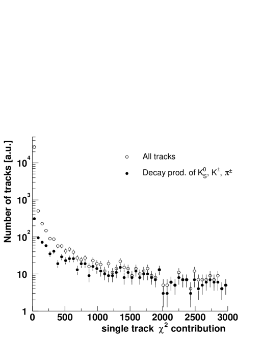
Figure 5.5: Distribution of single-track $\chi^{2}$-contributions, for all tracks (open circles) and tracks coming from decays of $\rm K^{0}_{S},\leavevmode\nobreak\ K^{\pm},\leavevmode\nobreak\ \pi^{\pm}$ (full circles).

In order to minimize the loss of resolution due to these effects, we apply a cut on the maximum contribution of a single track to the total $\chi^{2}$ of the fit, calculated as in (5.8). We proceed as follows: the fit is initially performed using all tracks and the $\chi^{2}$-contribution of each track w.r.t. the result of the fit is calculated; then the tracks whose contribution exceeds some value $\xi$ are removed and the fit is repeated. The process is iterated until no further tracks are removed or less than 3 tracks are left.

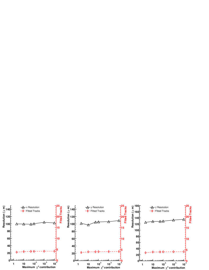
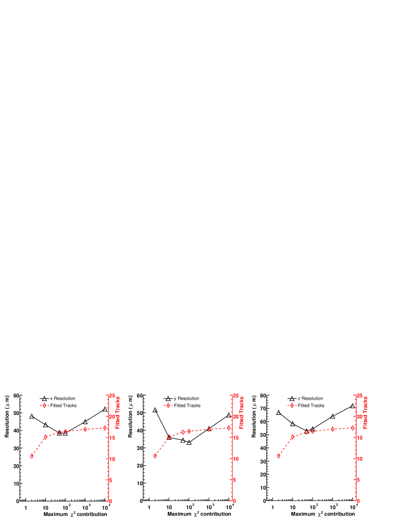
Figure 5.6: Tuning of the cut on the maximum $\chi^{2}$-contribution. Each plot presents the resolution on one of the three coordinates of the vertex ($x$, $y$ and $z$ from the left to the right) and the mean number of tracks included in the fit as a function of the cut. Top row: low-multiplicity events; central row: medium-multiplicity events; bottom row: high-multiplicity events.

The cut on $\xi$ has to be optimized in order to maximize the resolution of the fit. Indeed, if the cut is too loose, secondary or scattered tracks enter the fit and the resolution degrades; if the cut is too tight, primary tracks are removed and statistical precision is lost. The tuning has been done as a function of the number of reconstructed tracks in the event. The results are displayed in Fig. 5.6, where we present the resolutions on the three coordinates of the vertex together with the mean number of tracks used in the fit, as a function of the cut on $\xi$; as it can be seen from the number of tracks, in the top row we select low-multiplicity events, in the central row medium-multiplicity events and in the bottom row high-multiplicity events. At low multiplicity there is no dependence of the resolutions on the value of the cut, since there are essentially no secondary tracks in such events; while as the multiplicity increases, we observe the expected trend and the resolutions show a clear minimum.

Results for 3D vertex reconstruction

We tested the algorithm on the sample of pp events already described. Requiring a minimum of 3 tracks in the vertex fit, the vertex was reconstructed in about 65% of the events of the sample. It was verified that essentially all the events in which the vertex was not reconstructed had less than 3 found tracks (see Ref. [88]). The efficiency for vertex reconstruction as a function of event multiplicity will be detailed in the following.

Figure 5.9 presents the residuals $\Delta q$ for the three vertex coordinates ($q=x,\leavevmode\nobreak\ y,\leavevmode\nobreak\ z$), integrated over the full statistics. The distributions are clearly non-gaussian, since they are the convolution of many gaussian distributions with different dispersions, depending on the number of tracks used in each event for the fit. However, we fitted with a Gaussian the central part of the distributions, in order to quantify the global resolution. We obtain $\sigma_{x}\simeq\sigma_{y}\simeq 60\leavevmode\nobreak\ \mathrm{\mu m}$ and $\sigma_{z}\simeq 90\leavevmode\nobreak\ \mathrm{\mu m}$, in fair agreement with the expected values (Section 5.3.2). Such agreement emerges also from the fit of the distributions of $\Delta x\times\sqrt{N_{\rm tracks}/2}$ and $\Delta z\times\sqrt{N_{\rm tracks}}$, which should give the ‘resolution corresponding to 1 track’ (Fig. 5.9).

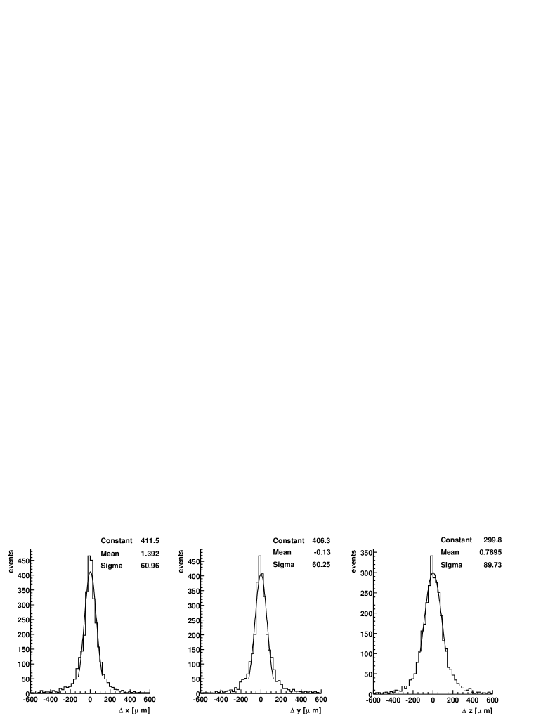
Figure 5.7: Distributions of the residuals: $\Delta q=q_{\rm measured}-q_{\rm true}$, for $q=x,\,y,\,z$.

Figure 5.8: Distributions of $\Delta x\times\sqrt{N_{\rm tracks}/2}$, $\Delta y\times\sqrt{N_{\rm tracks}/2}$ and $\Delta z\times\sqrt{N_{\rm tracks}}$. The width of these distributions gives the “resolution corresponding to 1 track”.

Figure 5.9: Distributions of the standardized residuals.

We checked the reliability of the estimated errors on the vertex position with the test of the pulls. The distribution of the standardized residuals, defined as $residual/\sqrt{variance}=\Delta q/\sqrt{\left\langle q,q\right\rangle}$ for $q=x,\,y,\,z$, are normal (mean $\simeq 0$, $\sigma\simeq 1$), as shown in Fig. 5.9; therefore, we conclude that the errors given in the vertex covariance matrix describe correctly the resolution on the vertex estimate.

These global results are summarized in Table 5.1.

Table 5.1: Summary table of the results on the vertex fit, integrated over all events.

Parameter		$x$	$y$	$z$
Resolution	[$\mathrm{\mu m}$]	61	60	90
Resolution per track	[$\mathrm{\mu m}$]	109	110	254
Pull		1.04	1.06	1.16

The sample was subdivided into five multiplicity (${\rm d}N_{\rm ch}/{\rm d}y$) classes in order to study the resolution and the efficiency of the method as a function of event multiplicity. The multiplicity was computed in the central pseudorapidity unit counting charged pions, charged kaons, protons, electrons and muons originating within $100\leavevmode\nobreak\ \mathrm{\mu m}$ from the primary vertex.

The efficiency for vertex reconstruction (defined as the ratio of the number of events with vertex found to the total number of events, in each bin) grows as a function of the multiplicity and it is saturated at 1 for ${\rm d}N_{\rm ch}/{\rm d}y>10$ (Fig. 5.11).

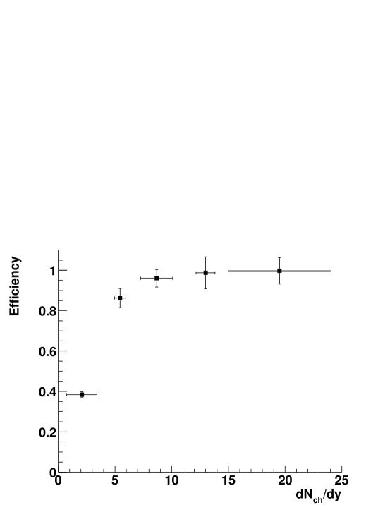
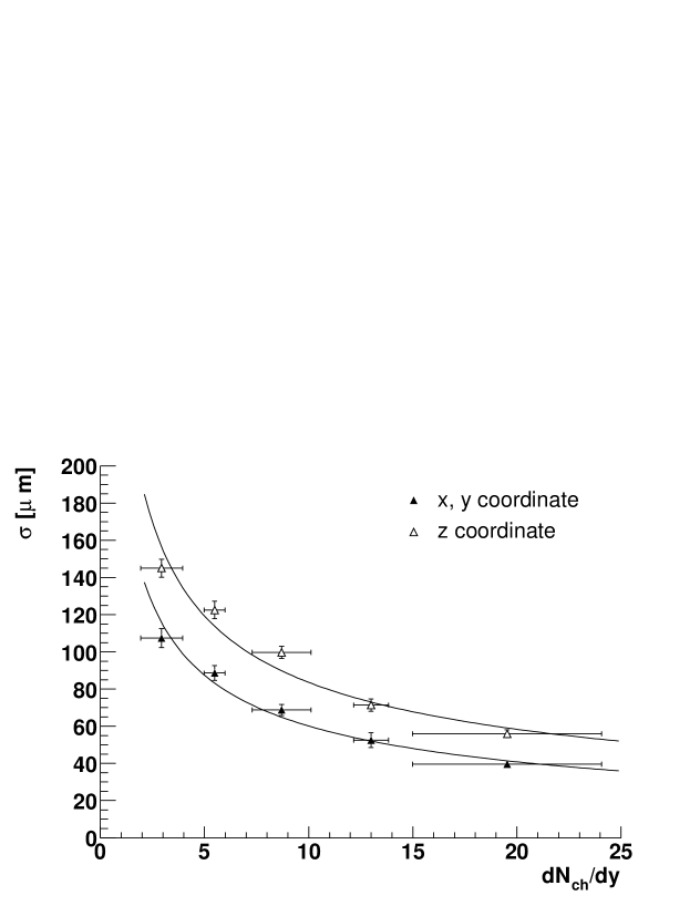
Figure 5.10: Fraction of events for which the vertex is reconstructed from the tracks, as a function of event multiplicity.

Figure 5.11: Resolutions on vertex position in $x$ and $z$ as a function of event multiplicity. The trends have been fitted to the expression $a+b/\sqrt{{\rm d}N_{\rm ch}/{\rm d}y}$ and the fitted parameters are reported in Table 5.2.

The resolutions as a function of the event multiplicity are shown in Fig. 5.11. As done for the $z$ measurement with the pixels, the resolutions were fitted to the expression:

$$\sigma({\rm d}N_{\rm ch}/{\rm d}y)=a+b\bigg{/}\sqrt{{\rm d}N_{\rm ch}/{\rm d}y}.$$ (5.11)

The results of the fit are reported in Table 5.2.

Table 5.2: Results of the fit of the multiplicity dependence of the resolutions to the expression $a+b/\sqrt{{\rm d}N_{\rm ch}/{\rm d}y}$.

Parameter		$x,\leavevmode\nobreak\ y$	$z$
$a$	$[\mathrm{\mu m}]$	$-6\pm 4$	$-3\pm 4$
$b$	$[\mathrm{\mu m}]$	$208\pm 13$	$272\pm 13$

We summarize the results for the reconstruction of the interaction vertex in pp collisions in Fig. 5.12, where the resolutions achieved for the $z$ coordinate with pixels, for the $z$ and $x$ ($y$) coordinates with tracks are displayed as a function of event multiplicity. The improvement on the $z$ resolution when using the tracks is of $\simeq 50\leavevmode\nobreak\ \mathrm{\mu m}$, but it increases at high ${\rm d}N_{\rm ch}/{\rm d}y$ as the average $p_{\rm t}$ of the reconstructed tracks increases with the multiplicity, and hence their average position resolution improves.

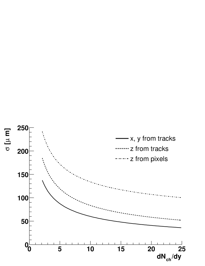
Figure 5.12: Summary plot for the achieved resolutions as a function of multiplicity.

5.4 Track impact parameter resolution in pp

Given the results presented in the former section, in proton–proton the impact parameter resolution has a significant contribution from the uncertainty on the primary vertex position, which is, on average, about one order of magnitude larger than in the Pb–Pb case.

The resolution on the track position in the transverse plane —the main contribution to the impact parameter resolution— is essentially the same in pp and in Pb–Pb if 6 ITS clusters are required (Fig. 5.14). This is not surprising, since we have already verified that the effect due to the presence of fake tracks in Pb–Pb is quite small (Section 5.2.2).

Let us now concentrate on the impact parameter resolution in the transverse plane ($r\phi$). The aim of the measurement of the tracks impact parameter is the identification of one or more displaced tracks with respect to the interaction vertex. Therefore, in pp collisions, we adopt the following strategy for the measurement of the impact parameter: the impact parameter of a given track $j$ is estimated as the distance of closest approach of the track $j$ to the vertex position obtained by excluding the track $j$ from the vertex reconstruction. In fact, if the track $j$ was included in the reconstruction, it would bias the vertex position, leading to a systematic underestimation of the impact parameter. This effect is shown in Fig. 5.14, where the following distributions are compared for primary pions with $p_{\rm t}\approx 1\leavevmode\nobreak\ \mathrm{GeV}/c$: impact parameter using true vertex position (solid), impact parameter using vertex estimated from all tracks (dashed), impact parameter using vertex estimated from all tracks but $j$ (dotted). In the case of the $\mbox{$\mathrm{D^{0}}$}\to\mbox{$\mathrm{K}$}^{-}\pi^{+}$ vertex reconstruction, as we will detail in Chapter 6, when we consider a given pair of tracks as a $\mathrm{D^{0}}$ candidate, we exclude both of them from the fit of the primary vertex.

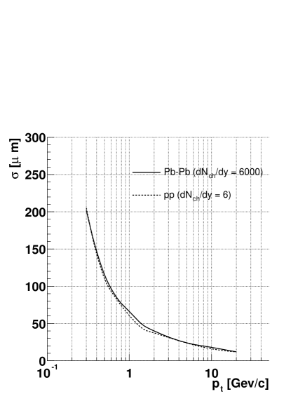
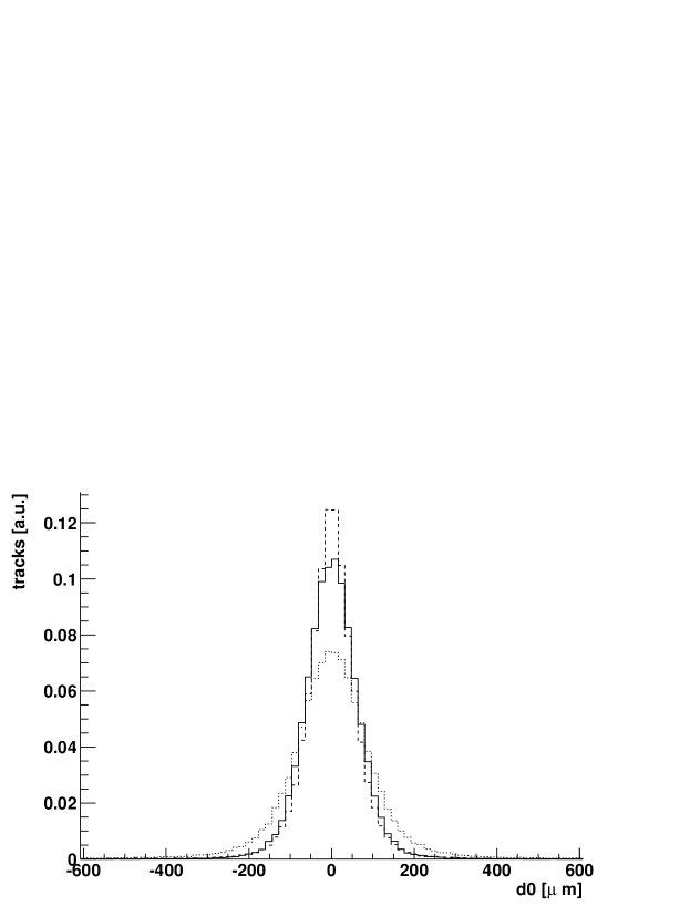
Figure 5.13: Resolution on the track position in the transverse plane in Pb–Pb and in pp for pions.

Figure 5.14: Distributions of the impact parameters for primary pions with $p_{\rm t}\approx 1\leavevmode\nobreak\ \mathrm{GeV}/c$ obtained: using true vertex position (solid), using vertex estimated from all tracks in the event (dashed), using vertex estimated from all tracks but the current one (dotted).

Figure 5.15 presents the impact parameter resolution as a function of the transverse momentum obtained with this strategy. We considered primary pions reconstructed in TPC and ITS, with 6 points in the ITS layers. We used a sample of $7.5\cdot 10^{6}$ PYTHIA events, in order to have sufficient statistics at high transverse momentum. In the top-left panel, we show the resolution integrated over all events (for this sample the average number of reconstructed tracks is $\left\langle N_{\rm tracks}\right\rangle=7$). Then, we consider only events with $N_{\rm tracks}\geq N_{\rm min}$, with $N_{\rm min}=10,\,15,\,20$. We plot the resolution $\sigma(d_{0})$ on the impact parameter (solid line), the resolution $\sigma_{\rm track}$ on the track position (dashed line) and an ‘equivalent resolution’ on the vertex position (dotted line), calculated, ‘inverting’ the expression (5.3), as:

$$\sigma_{\rm vertex}=\sqrt{\sigma(d_{0})^{2}-\sigma_{\rm track}^{2}}$$ (5.12)

(for all quantities we consider the $r\phi$ component).

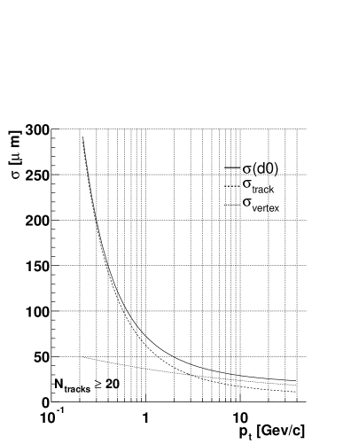
Figure 5.15: Impact parameter resolution in the bending plane as function of the transverse momentum in pp collisions. The panels differ in the minimum number of reconstructed tracks required (see text).

From the analysis of these plots, we observe the following:

• the worsening in the $d_{0}$ resolution w.r.t. the case of perfect knowledge of the vertex position, $[\sigma(d_{0})-\sigma_{\rm track}]/\sigma_{\rm track}$, is negligible for very-low-$p_{\rm t}$ tracks, of the order of $30\%$ for $p_{\rm t}=1\leavevmode\nobreak\ \mathrm{GeV}/c$ and of the order of $50\%$ for $p_{\rm t}=10\leavevmode\nobreak\ \mathrm{GeV}/c$;

• the impact of the uncertainty on the vertex position is not too dramatic for medium- and high-momentum tracks, since these tracks are always produced in events with large multiplicity, in which the vertex can be reconstructed quite precisely; this is clearly shown by the strong $p_{\rm t}$-dependence of the equivalent vertex resolution, $\sigma_{\rm vertex}$;

• as the number of reconstructed tracks (i.e. the multiplicity of the event) increases, the impact of the uncertainty on the vertex position becomes smaller: for a track with $p_{\rm t}=1\leavevmode\nobreak\ \mathrm{GeV}/c$ it becomes $20\%$ if the total number of tracks is $\geq 10$ and $15\%$ if the total number of tracks is $\geq 15$.

We, therefore, conclude that the algorithm for vertex reconstruction in pp collisions allows the measurement of the impact parameter projection in the bending plane with a resolution that is not substantially worse than the track position resolution for low and medium transverse momentum tracks, in particular for tracks produced in high-multiplicity events. To this respect, we observe that, indeed, events with heavy flavour production have a multiplicity which is larger than the mean multiplicity in pp minimum-bias events. We will discuss and quantify this observation in Chapter 6. For high-momentum tracks the achieved impact parameter resolution is roughly twice the track position resolution; however, this is not dramatic, since, at high $p_{\rm t}$, the background to heavy flavour particles is almost negligible and, therefore, the selection based on the impact parameter is not as crucial as it is for low-momentum particles.

5.5 Secondary vertex reconstruction

The knowledge of the position of the secondary vertex allows the complete reconstruction of the momentum of the particle that has decayed. This provides an effective selection handle, because it allows to require the pointing of the momentum to the main interaction vertex. Moreover, a direct measurement of the $p_{\rm t}$ distribution (of charm particles, for example) is possible.

For a given pair of opposite-sign tracks the secondary vertex is reconstructed by a minimization of the distance in space between the two helices representing the tracks. Once the ‘minimum segment’ between the tracks is found, the position of the vertex on this segment is defined keeping into account the different position precision of the two tracks. This information can be retrieved from the track covariance matrix. As we have seen in the section on the impact parameter resolution, the track with the largest momentum has a better precision and, therefore, the vertex is usually estimated to be closer to this track than to the lower-momentum one. This method was originally developed for the reconstruction of strange particle decays (namely, ${\rm K^{0}_{S}}$, $\Lambda$, $\Xi$ and $\Omega$) and it was adopted also for the reconstruction of $\mathrm{D^{0}}$ decays.

Figure 5.16 reports the resolutions on the three coordinates of the secondary vertex, as a function of the transverse momentum of the $\mathrm{D^{0}}$. There is clearly a strong correlation with the impact parameter resolution: the resolution is better in the bending plane ($x$ and $y$) than in $z$ and, for $p_{\rm t}<2$-$3\leavevmode\nobreak\ \mathrm{GeV}/c$, it improves as $p_{\rm t}$ increases. We will comment later on the worsening observed at high $p_{\rm t}$ for the $x$ and $y$ coordinates. We can first try to understand quantitatively the obtained resolutions.

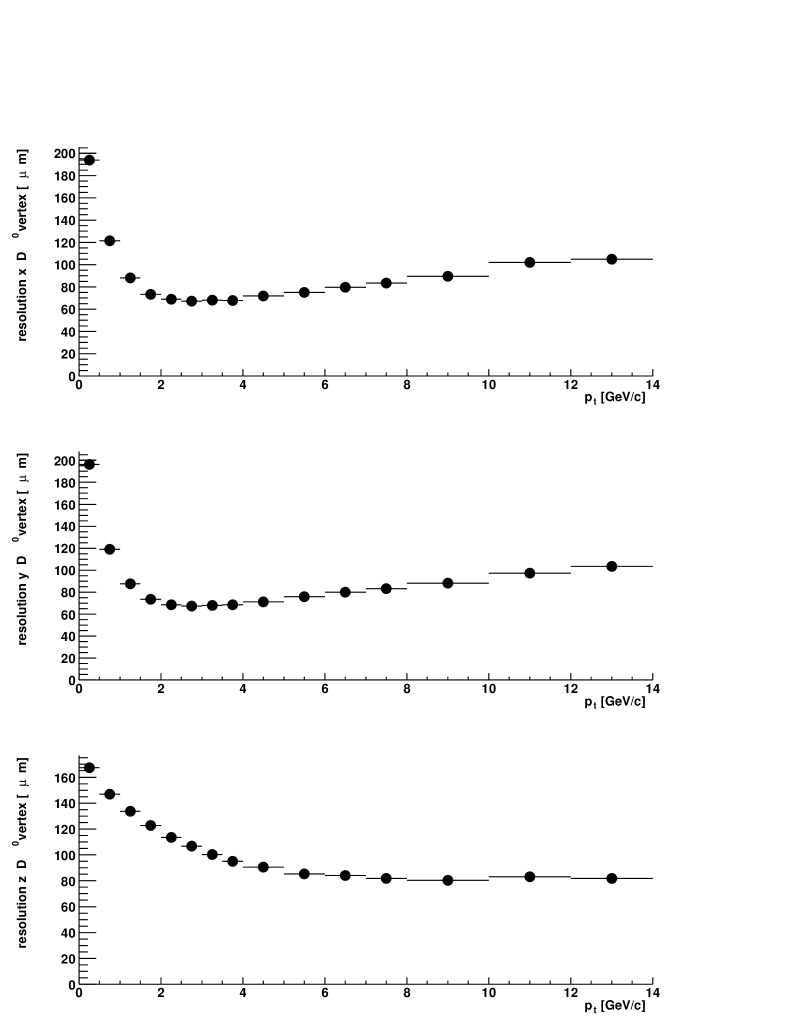
Figure 5.16: Resolution on the three coordinates ($x,\leavevmode\nobreak\ y,\leavevmode\nobreak\ z,$ from top to bottom) of the position of the $\mathrm{D^{0}}$ decay vertex, as a function of the transverse momentum of the $\mathrm{D^{0}}$.

We concentrate on the values at $p_{\rm t}\simeq 2\leavevmode\nobreak\ \mathrm{GeV}/c$, which is the average $p_{\rm t}$ of the $\mathrm{D^{0}}$ particles produced at the LHC, as we have seen in Section 3.5. The average $p_{\rm t}$ of the decay products is $\simeq 1\leavevmode\nobreak\ \mathrm{GeV}/c$. If the opening angle between the two decay tracks is not too small, we can consider each track to ‘measure’ one of two perpendicular coordinates in the bending plane; in this way, we expect a resolution of the order of the impact parameter resolution in $r\phi$ at $p_{\rm t}\simeq 1\leavevmode\nobreak\ \mathrm{GeV}/c$, i.e. $\simeq 50$-$70\leavevmode\nobreak\ \mathrm{\mu m}$. Along the $z$ direction, both tracks contribute to the measurement of the secondary vertex position; thus, we expect a resolution of $\simeq\sigma(d_{0}(z))_{p_{\rm t}\simeq 1\leavevmode\nobreak\ \mathrm{GeV}/c}/\sqrt{2}\simeq 100$-$120\leavevmode\nobreak\ \mathrm{\mu m}$. The observed resolutions at $p_{\rm t}=2\leavevmode\nobreak\ \mathrm{GeV}/c$ agree with these simple estimates.

At higher $p_{\rm t}$ the resolution in the bending plane worsens as $p_{\rm t}$ increases: this is due to the fact that the angle between the two decay tracks becomes smaller as the $p_{\rm t}$ of the $\mathrm{D^{0}}$ increases and, thus, the two coordinates $x$ and $y$ are measured using essentially only 1 track. The expected resolution per coordinate in this case is $\simeq\sigma(d_{0}(r\phi))_{p_{\rm t}\simeq 1\leavevmode\nobreak\ \mathrm{GeV}/c}/\sqrt{0.5}\simeq 80$-$90\leavevmode\nobreak\ \mathrm{\mu m}$.  

In the first detailed study for the $\mathrm{D^{0}}$ detection [90] a different method for the reconstruction of the secondary vertex was used. The two tracks were approximated to straight lines starting from the intersection point of the circles obtained projecting the tracks on the bending plane. The secondary vertex was defined as the middle-point of the shortest segment joining the two lines.

It is interesting to compare the results, in terms of position resolution, given by the two different methods. In Fig. 5.17 we report, for the two methods, the distances in space and in the bending plane between the reconstructed and the true vertex. The achieved resolutions are very similar in the two cases, allowing to conclude that there is no much room for further optimization.

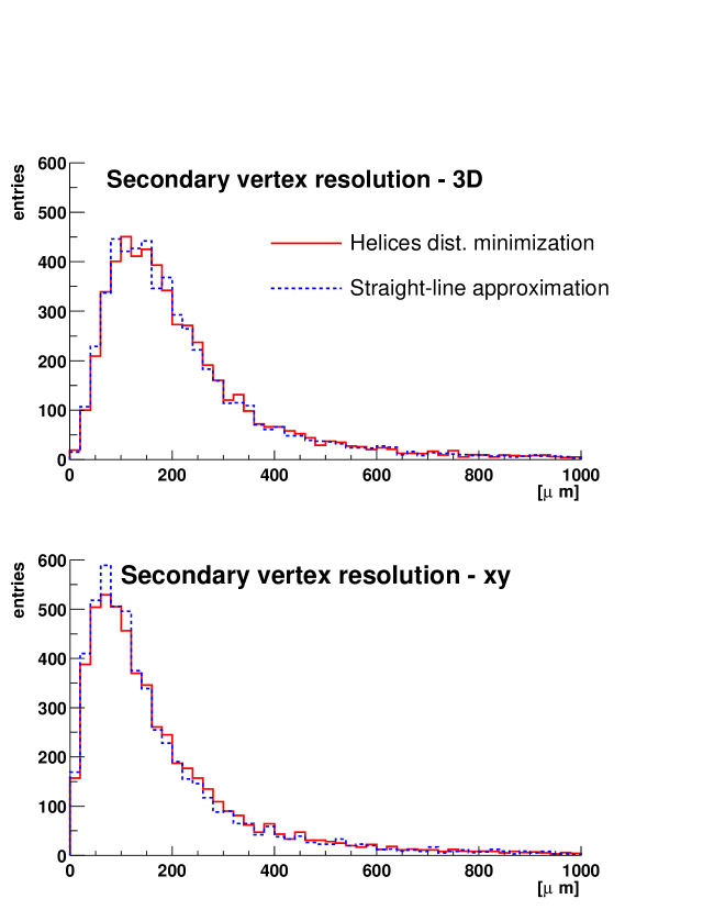
Figure 5.17: Distance between the reconstructed and the true position of the secondary vertex for the two reconstruction methods: minimization of the distance between helices (solid) and straight-line approximation of the tracks (dashed). Both the distance in space (top) and in the bending plane (bottom) are shown.

Chapter 6 Exclusive reconstruction of $\mathrm{D^{0}}$ particles

In Chapter 2 we have shown that the exclusive reconstruction of charm mesons is a very effective tool to study the production of charm quarks in nucleus–nucleus collisions at the LHC and we have outlined a detection strategy for the decay ${\rm D^{0}\to K^{-}\pi^{+}}$. In Chapters 4 and 5 we have described the ALICE experimental apparatus and shown how its capabilities for tracking and vertexing allow to pursue this measurement. This chapter presents the details and results of the feasibility study, that was carried out for both the Pb–Pb and the pp case. The study done for Pb–Pb collisions is described in the first part of the chapter (Section 6.1). Then, the proton–proton case is addressed (Section 6.2) with particular emphasis on the aspects that are distinctive of the low multiplicity of pp events. The results obtained for Pb–Pb and pp are compared at various stages of the reconstruction and selection chain in order to check their consistency and understand their differences.

6.1 Feasibility study for Pb–Pb collisions

As discussed in Chapter 2, in nucleus–nucleus collisions the signal of the $\mathrm{D^{0}}$ hadronic decay has to be selected out of a very large combinatorial background (proportional to the square of the charged particle rapidity density ${\rm d}N_{\rm ch}/{\rm d}y$) given by pairs of uncorrelated tracks with large impact parameters. These can be:

1. primary tracks which acquire an impact parameter due to scatterings in the material of the beam pipe and of the innermost pixel layer;

2. tracks from the decays of hyperons ($\Lambda$, $\Xi$, $\Omega$) and kaons;

3. tracks from undetected charm decays;

4. pions produced by annihilations of primary anti-protons ($\rm\overline{p}$) and anti-neutrons ($\rm\overline{n}$) in the beam pipe and in the innermost pixel layer.

As we will see, we have $S/B\sim 10^{-6}$ in the mass range $M_{\rm D^{0}}\pm 3\leavevmode\nobreak\ \sigma$, before selections; therefore, in order to extract the charm signal with good significance, one has to apply cuts selective enough to reduce the background by $6$-$7$ orders of magnitude. In view of this severe selection procedure, the required statistics for the study of the background and of the signal is very large ($\sim 10^{5}$ events for the background). Thus, we adopted a number of fast simulation techniques; namely:

• separate generation of signal and background events;

• event mixing technique to increase the statistics of the background;

• parameterization of track reconstruction in the TPC (this tool, described in Section 4.2.3 and in Ref. [85], was specifically developed in the scope of the charm studies presented here);

• fast simulation of the response of the ITS detectors (fast points);

• parameterization of the particle identification (PID) in the TOF detector.

6.1.1 Background and signal generation

Background

We chose to use the HIJING event generator, introduced in Section 4.2.1, for the simulation of Pb–Pb events, because it includes all the background sources listed above. This is not true, for example, for some parameterized generators, where the event multiplicity can be adjusted by the user but only primary pion and kaon tracks are provided. We have seen in Section 4.2.1 that the multiplicity given by HIJING when parton energy loss is included is ${\rm d}N_{\rm ch}/{\rm d}y\simeq 6000$, for central Pb–Pb collisions. Since the recent extrapolations from the RHIC measurements give values of the order of $2000$-$3000$ charged particles per unit of rapidity (Section 1.4.1), the number obtained in HIJING can be considered conservative. An extrapolation of the results to the case of lower multiplicity is presented in the last part of this section.

The collision impact parameter $b$ was sampled from the physical distribution d$N/$d$b\propto b$ and the condition $b<2\leavevmode\nobreak\ \mathrm{fm}$ was applied in order to generate central collisions.

Our background sample consists of $2\cdot 10^{4}$ such events, that were generated in 1000 sub-samples of 20 events each, the events of a sub-sample having the same values for the impact parameter $b$ and for the three coordinates of the primary vertex. Since the background is combinatorial, 400 equivalent events were obtained out of each sub-sample by combining each positive track of the sub-sample with all negative tracks of the sub-sample. In this way, $4\cdot 10^{5}$ equivalent events were obtained, increasing the background statistics by a factor 20.

Signal: ${\rm c}\to\mbox{${\rm D^{0}\to K^{-}\pi^{+}}$}$ and ${\rm b}\to{\rm B}\to\mbox{${\rm D^{0}\to K^{-}\pi^{+}}$}$

At LHC energies the ratio of the production cross sections for beauty and for charm is of the order of 5% (see Section 3.1). Considering also that the average inclusive branching ratio of B mesons to $\mathrm{D^{0}}$ is $\simeq 65\%$ [60], we conclude that a significant fraction of all produced $\mathrm{D^{0}}$ particles comes from b quarks (${\rm b}\to{\rm B}\to\mbox{$\mathrm{D^{0}}$}$). The ratio ($\mathrm{D^{0}}$ from b)/($\mathrm{D^{0}}$ from c) can be calculated as:

$$\frac{{\rm d}N({\rm b}\to{\rm B}\to\mbox{$\mathrm{D^{0}}$})/{\rm d}y}{{\rm d}N({\rm c}\to\mbox{$\mathrm{D^{0}}$})/{\rm d}y}=\frac{{\rm d}N({\rm b}\to{\rm B^{0},B^{+}})/{\rm d}y\times BR({\rm B^{0},B^{+}\to\mbox{$\mathrm{D^{0}}$}})}{{\rm d}N({\rm c}\to\mbox{$\mathrm{D^{0}}$})/{\rm d}y}=$$

$$=\left\{\begin{array}[]{ll}0.049&{\rm for}\leavevmode\nobreak\ \mbox{Pb--Pb}\leavevmode\nobreak\ {\rm at}\leavevmode\nobreak\ \sqrt{s_{\scriptscriptstyle{{\rm NN}}}}=5.5\leavevmode\nobreak\ \mathrm{TeV}\\ 0.054&{\rm for}\leavevmode\nobreak\ {\rm pp}\leavevmode\nobreak\ {\rm at}\leavevmode\nobreak\ \sqrt{s}=14\leavevmode\nobreak\ \mathrm{TeV}\end{array}\right.$$

where the rapidity densities are taken from Tables 3.8 and 3.8. This ‘B contribution’ was included in the study presented here, since it is important to understand how the ratio of secondary (from b) to primary (from c) $\mathrm{D^{0}}$ is affected by the selections that we apply. After the selections this contribution has to be corrected for by subtracting, in bins of transverse momentum, the estimated number of secondary $\mathrm{D^{0}}$. As we will discuss in the next chapter, the uncertainty on this number, which is proportional to the uncertainty on the beauty cross section and to the fraction of secondary-to-primary $\mathrm{D^{0}}$, is one of the main contributions to the final systematic error. It is, therefore, essential to keep under control and, possibly, low this fraction. This is also motivated by the fact that, since the $p_{\rm t}$ distribution of b quarks is harder than that of c quarks and the selections will naturally tend to be more efficient for larger momenta, we expect the fraction secondary/primary $\mathrm{D^{0}}$ to increase after the selections.

The signal was generated using PYTHIA, tuned to reproduce the $p_{\rm t}$ distribution of charm and beauty quarks given by the NLO calculations by Mangano, Nason and Ridolfi, as explained in Section 3.4. Many $\mbox{$\mathrm{D^{0}}$}/\overline{\mbox{$\mathrm{D^{0}}$}}$ mesons, with decay forced in a charged $\mbox{$\mathrm{K}$}\pi$ pair, were superimposed in special ‘signal events’. The number of $\mathrm{D^{0}}$ per event (13000 in $|y|<2$) was tuned in order to have the same track multiplicity as in a central HIJING event. In this way, the $\mathrm{D^{0}}$ decay products are reconstructed with the same efficiency as if they were produced in a central Pb–Pb collision. It was verified that the different momentum and impact parameter distributions of these ‘signal events’ with respect to central HIJING events do not affect significantly the reconstruction efficiency (more details are given Section 6.1.2).

A total of 1000 such ‘signal events’ were generated with primary $\mathrm{D^{0}}$ particles. Using our present rate estimate (from Table 3.8) and a branching ratio of $3.8\%$ [60], such a number of ${\rm D^{0}\to K^{-}\pi^{+}}$ decays corresponds to $\simeq 6.1\cdot 10^{6}$ central Pb–Pb events. In addition, we have generated 49 similar events, but with secondary $\mathrm{D^{0}}$ from the decay of B mesons. In this case we set PYTHIA in order to reproduce the NLO pQCD results for the $p_{\rm t}$ distribution of b quarks. We did not transport through the detector the other decay products of the b quarks and of the B mesons, but only the kaons and pions from the $\mathrm{D^{0}}$ decays. Figure 6.1 shows the $p_{\rm t}$ distributions for primary and secondary $\mathrm{D^{0}}$ mesons: as expected the latter have a harder spectrum.

All the results presented here are scaled to $10^{7}$ central Pb–Pb events, expected to be collected in the 1-month heavy ion run of 1 LHC year.

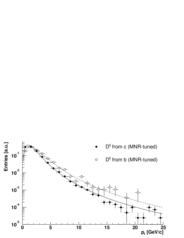
Figure 6.1: Transverse momentum distributions for primary and secondary (from B meson decays) $\mathrm{D^{0}}$ mesons, in Pb–Pb collisions at $5.5\leavevmode\nobreak\ \mathrm{TeV}$.

Interaction vertex

For both signal and background events, the $x$ and $y$ coordinates of the vertex were sampled from two gaussian distributions with $\sigma=15\leavevmode\nobreak\ \mathrm{\mu m}$ and centred at $(0,0)$, while the $z$ position was sampled from a Gaussian with $\sigma=5.3\leavevmode\nobreak\ \mathrm{cm}$, according to the expected beam configuration during the heavy ion running (Section 4.3.2). A cut at $\pm 1\leavevmode\nobreak\ \sigma$ on the $z$ position of the vertex was applied; this corresponds to the expected width of the fiducial interaction region.

6.1.2 Detector simulation and event reconstruction

The detector simulation was done in the framework of AliRoot, as described in Section 4.2.2, using a detailed description of the materials for the beam pipe and the ITS, which are instrumental in determining track impact parameters and secondary vertices positions, the crucial quantities to extract the charm signal. The response of the TPC was parameterized and in Appendix C we show that this does not affect the momentum and impact parameter resolutions obtained after completing the track reconstruction in the ITS. In order to contain the CPU time and storage space within reasonable limits, the fast points were used in the ITS (Section 4.2.3); in Chapter 5, Fig. 5.3, we have shown that this approximation does not affect the impact parameter resolution. Also the particle identification response of the Time Of Flight detector was parameterized, as we shall detail in the next section.

The value of the magnetic field used in the simulation was $B=0.4$ T, which is close to the maximum value that can be provided by the ALICE magnet. This kind of physics studies yields better performance with relatively large values of the magnetic field, since (a) the invariant mass resolution is better with larger fields and (b) the acceptance at very low $p_{\rm t}$ ($<500\leavevmode\nobreak\ \mathrm{MeV}/c$) is not crucial. The extrapolation of the results for lower values of the magnetic field is straight-forward and will be eventually discussed.

The $z$ position of primary vertex was reconstructed for each event by means of the Silicon Pixel Detectors using the method briefly described in Section 5.1 (see Refs. [86, 87] for the details). We remind that a resolution of $\simeq 6\leavevmode\nobreak\ \mathrm{\mu m}$ is obtained with ${\rm d}N_{\rm ch}/{\rm d}y=6000$. The vertex position in the transverse plane was taken at the nominal value $(0,0)$, i.e. it was assumed to be known within the uncertainty given by the size of the interaction region ($\simeq 15\leavevmode\nobreak\ \mathrm{\mu m}$).

Track reconstruction in the ITS was performed as described in Section 4.2.3, using as input for the standard Kalman filter the parameterized tracks of the TPC. At least 5 clusters per track were required in the ITS, including the clusters in the two pixel layers; as shown in Section 5.2.2, in this way the impact parameter resolution is still optimal.

The reconstruction was performed in the same way for background and ‘signal events’. Figure 6.2 demonstrates that the tracking efficiency as a function of $p_{\rm t}$ in the ITS for the ‘signal events’ is the same as for the background events.

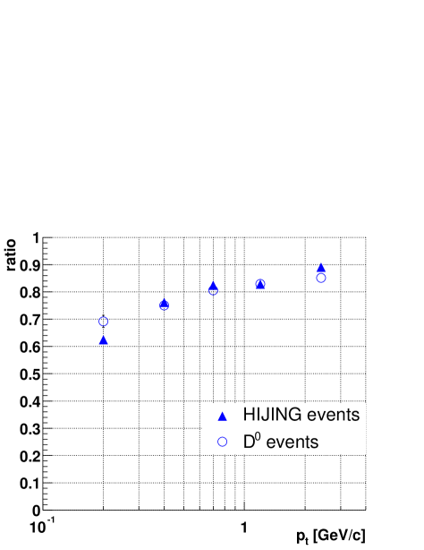
Figure 6.2: ITS tracking efficiency, defined as the ratio between the number of tracks reconstructed in the ITS with respect to the number of tracks reconstructed in the TPC, as a function of $p_{\rm t}$ for central HIJING events and for ‘signal events’ containing only $\mbox{$\mathrm{D^{0}}$}/\overline{\mbox{$\mathrm{D^{0}}$}}$, decaying in $\mbox{$\mathrm{K}$}\pi$, with the same track multiplicity as a central HIJING event.

6.1.3 Particle identification in the TOF detector

In the momentum range of interest for charm analysis ($p\simeq 0.5$-$2\leavevmode\nobreak\ \mathrm{GeV}/c$) the particle identification capability of ALICE is determined mainly by the TOF detector. The measurement of the time-of-flight $t$ across a known distance $L$ for a track with momentum $p$ (measured in the TPC and in the ITS) allows an estimation of the particle mass as:

$$m=p\cdot\sqrt{\frac{t^{2}}{L^{2}}-1}.$$ (6.2)

Figure 6.3 presents a scatter plot of the measured momenta versus the estimated masses for the particles produced in central Pb–Pb collisions generated with HIJING. The points corresponding to electrons, pions, kaons and protons are coloured in red, yellow, blue and green, respectively. The figure, from the TOF Technical Design Report (TDR) [91], is obtained for $B=0.4$ T assuming an overall time resolution of $150$ ps. The association of the time-of-flight and, hence, of the mass to a specific reconstructed track is obtained by means of a matching algorithm, that propagates the track from the outer radius of the TPC to the TOF detector and matches it with one of the $\approx 3\times 3\leavevmode\nobreak\ \mathrm{cm}^{2}$ pads of the detector [91]. Tracks matched with a non-active region of the detector or with a non-fired or multi-fired pad are not assigned a mass. The TRD, which lies between the TPC and the TOF, will provide a ‘bridge’ between the two detectors and improve the matching procedure. Since the extension of track reconstruction to the TRD is still under development, Fig. 6.3 was obtained from a simulation that does not include the material of the TRD. Indeed, it would be too pessimistic to consider the TRD as a layer of inactive material.

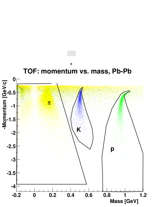
Figure 6.3: Momentum versus mass calculated from TOF for a sample of HIJING Pb–Pb events. The lines correspond to the chosen graphical cuts relative to the selection of pions, kaons and protons. Negative values of the mass are assigned when the argument of the square root in equation 6.2 is lower than 0.

For $0.5<p<2$-$2.5\leavevmode\nobreak\ \mathrm{GeV}/c$ there is a good mass separation of pions, kaons and protons. For lower momenta the matching tends to fail because of multiple scattering and energy loss, while for $p>2$-$2.5\leavevmode\nobreak\ \mathrm{GeV}/c$ the separation vanishes, especially between pions and kaons, as they become relativistic.

The association of the particle type to a track (tagging) is determined by applying cuts on the momentum-versus-mass plane. The values of these cuts determine the identification efficiency and the contamination of the sample. The identification efficiency for a particle type $i$ is defined as the ratio of the number of tracks of type $i$ correctly tagged as $i$ to the total number of tracks of type $i$; the contamination is defined as the ratio of the number of tracks incorrectly tagged as $i$ to the total number of tracks tagged as $i$. The optimal level of contamination and efficiency depends on the specific physics case under study.

We divide our set of reconstructed tracks into four samples: those identified as pions ($\pi_{\rm tag}$), as kaons ($\mbox{$\mathrm{K}$}_{\rm tag}$), as protons (${\rm p}_{\rm tag}$) and non-identified ($?_{\rm tag}$). A ${\rm D^{0}\to K^{-}\pi^{+}}$ decay for which both the pion and the kaon tracks are reconstructed corresponds to a pair of tracks of opposite charge $(-,+)$. According to their PID, the pair can fall in one of the following samples:

Sample A

($\mbox{$\mathrm{K}$}_{\rm tag}$, $\pi_{\rm tag}$) + ($\mbox{$\mathrm{K}$}_{\rm tag}$, $?_{\rm tag}$): the kaon is identified while the other track can be identified as pion or non-identified;

Sample B

($?_{\rm tag}$, $\pi_{\rm tag}$): only the positive track is identified as pion;

Sample C

($?_{\rm tag}$, $?_{\rm tag}$): both tracks are not identified; in this sample each pair is counted twice: once as a $\mathrm{D^{0}}$ candidate and once as a $\overline{\mbox{$\mathrm{D^{0}}$}}$ candidate.

Sample D

All other combinations, like e.g. ($\pi_{\rm tag}$, $\pi_{\rm tag}$). These pairs are rejected.

If the pion from a $\mathrm{D^{0}}$ decay is correctly identified, but the kaon is misidentified as a pion, the candidate falls in sample D and is lost. Therefore, for open charm detection, the PID strategy has to be optimized in order to minimize the number of kaons tagged as pions, while tagging correctly a large fraction of the pions.

On the basis of this guideline the PID tags have been defined in the following way:

• any track not matched with a single-fired TOF pad is tagged as $?_{\rm tag}$;

• tracks matched with a single-fired TOF pad are tagged according to the graphical cuts shown in Fig. 6.3; if a track falls outside all graphical cuts it is tagged as $?_{\rm tag}$.

The graphical cuts were optimized in order to minimize the probability to tag a kaon as a pion, i.e. to minimize the loss of signal.

In this way, for every particle type, we can compute the probabilities to be tagged as pion, kaon, proton or non-identified. These probabilities are shown in Fig. 6.4 as a function of the total momentum. We give an example of how these figures should be read: for a reconstructed track (in TPC and ITS), known from the simulation to be a kaon, with $p=1\leavevmode\nobreak\ \mathrm{GeV}/c$, the probability to be tagged as kaon is 45%, the probability to tagged as pion is 8% and the probability to be tagged as non-identified is the remaining 47% (see central panel).

In our study the TOF detector was not included in the simulation of all the events and the three samples A, B and C were populated with $\mathrm{D^{0}}$ candidates according to the tabulated probabilities from the figure, both for the signal and for the background. The PID information was used for $p<2\leavevmode\nobreak\ \mathrm{GeV}/c$ for pions and kaons and for $p<4\leavevmode\nobreak\ \mathrm{GeV}/c$ for protons; for larger momenta all tracks were tagged as $?_{\rm tag}$ (non-id). The fraction of signal lost because the kaon is tagged as a pion is 10%.

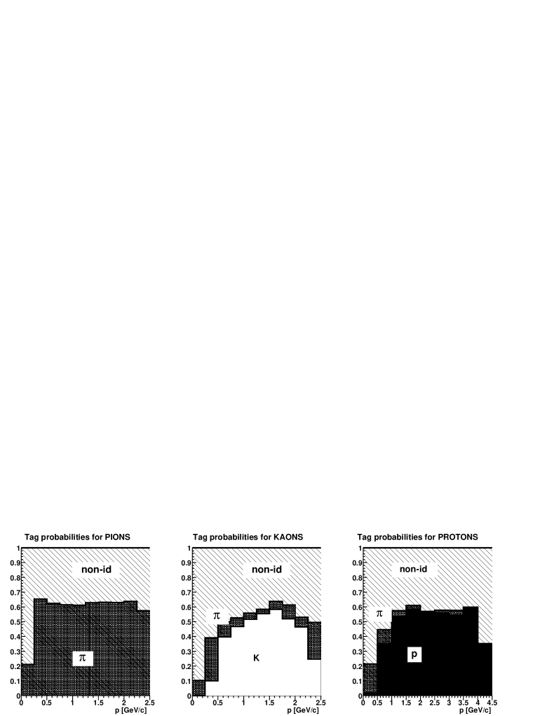
Figure 6.4: PID tag probabilities for reconstructed pions, kaons and protons in Pb–Pb collisions with the TOF detector.

6.1.4 Analysis

For each $\mathrm{D^{0}}$ candidate (opposite-charge tracks pair) the position of the decay vertex is computed, as explained in Section 5.5, by a minimization of the distance in space between the two helices representing the particle trajectories. The momentum of the $\mathrm{D^{0}}$ candidate is calculated as the sum of the momenta of the kaon and of the pion at the position of closest approach between the two tracks. The invariant mass of the pair is calculated as $M=\sqrt{(E_{+}+E_{-})^{2}-(\vec{p}_{+}+\vec{p}_{-})^{2}}$ and, for the signal, the resolution $\sigma$ for $B=0.4$ T is reported in Fig. 6.5 as a function of the $\mathrm{D^{0}}$ transverse momentum. The average resolution is $12\leavevmode\nobreak\ \mathrm{MeV}$ and the $p_{\rm t}$ dependence reflects the trend of the momentum resolution (Fig. 4.9).

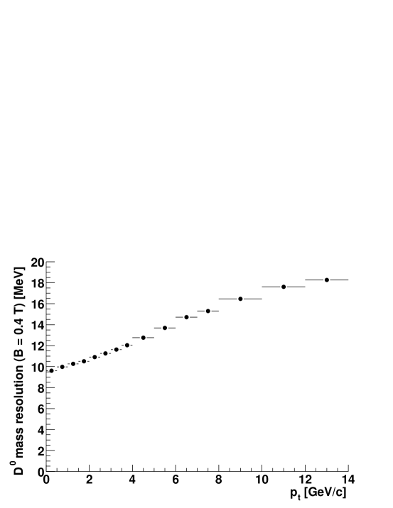
Figure 6.5: $\mathrm{D^{0}}$ invariant mass resolution as a function of $p_{\rm t}$, for $B=0.4$ T.

In Table 6.1 we present the signal-to-background ratios for the three samples A, B and C in the invariant mass range $|M_{\rm K\pi}-M_{\rm D^{0}}|<3\leavevmode\nobreak\ \sigma$, before any geometrical or kinematical selection. Due to the small fraction of kaons in the background, sample A (kaon identification required) shows the highest $S/B$ ratio ($\sim 2\cdot 10^{-5}$). However, Fig. 6.4 (central panel) shows that the identification probability decreases rapidly for kaons with momentum larger than $1.5\leavevmode\nobreak\ \mathrm{GeV}/c$; therefore, for $\mathrm{D^{0}}$ momenta larger than $\sim 2$-$3\leavevmode\nobreak\ \mathrm{GeV}/c$, the fraction of signal that populates sample A becomes marginal. For this reason, we consider as our standard sample the sum of the three samples A, B and C (called ‘Total’ in Table 6.1); this corresponds to the rejection of ($\pi_{\rm tag}$, $\pi_{\rm tag}$) and ($\mbox{$\mathrm{K}$}_{\rm tag}$, $\mbox{$\mathrm{K}$}_{\rm tag}$) pairs. In the low-$p_{\rm t}$ region, it will be eventually convenient to restrict the PID selection to sample A only.

Table 6.1: Initial values of $S/B$ in the invariant mass range $M_{\rm D^{0}}\pm 3\leavevmode\nobreak\ \sigma$, before selection.

Sample	$S$/event	$B$/event	$S/B$
A	$0.054$	$2.5\cdot 10^{3}$	$2.16\cdot 10^{-5}$
B	$0.041$	$1.4\cdot 10^{4}$	$2.98\cdot 10^{-6}$
C	$0.031$	$1.2\cdot 10^{4}$	$2.69\cdot 10^{-6}$
Total	$0.126$	$2.8\cdot 10^{4}$	$4.53\cdot 10^{-6}$

Several selection cuts are applied in order to increase the $S/B$ ratio to the level needed to extract the signal. Their definition is presented in the following paragraphs.

Pairs for which the distance of closest approach ($dca$) between the tracks is larger than $dca_{\rm max}$ ($300$-$400\leavevmode\nobreak\ \mathrm{\mu m}$, depending on the transverse momentum of the $\mathrm{D^{0}}$ candidate) are rejected.

Since the transverse momentum distributions for the signal are harder than those for the background, it is convenient to apply a cut on the minimum $p_{\rm t}$ for $\mathrm{K}$ and $\pi$ ($p_{\rm t}>800\leavevmode\nobreak\ \mathrm{MeV}/c$).

In the reference frame of the decaying $\mathrm{D^{0}}$, we define $\theta^{\star}$ as the angle between the pion momentum and the $\mathrm{D^{0}}$ flight line (see sketch in Fig. 6.6). As shown in Fig. 6.6 (right), the background accumulates at $\cos\theta^{\star}=\pm 1$. The distribution for the signal is not uniform due to the other cuts applied, in particular the cut on the minimum $p_{\rm t}$ of the pion and of the kaon. The slight asymmetry reflects the different masses of the kaon and the pion. Only pairs with $|\cos\theta^{\star}|<cth_{\rm max}$ ($\simeq 0.6$) are kept.

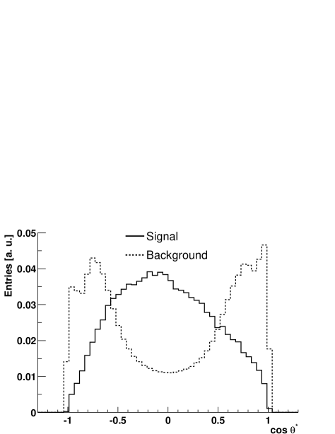
Figure 6.6: Definition of the decay angle $\theta^{\star}$ in the $\mathrm{D^{0}}$ reference frame (left). On the right, distribution of $\cos\theta^{\star}$ for the $\mathrm{D^{0}}$ signal (solid line) and for the background (dashed line). The histograms are normalized to the same integral.

With these cuts the signal-to-background ratio increases by a factor $\sim 100$. Further improvement can be obtained by applying the displaced vertex identification procedure, outlined in Section 2.5.1, based on the impact parameter and on the requirement that the reconstructed $\mathrm{D^{0}}$ points back to the primary vertex.

We consider only the impact parameter projection on the transverse plane ($d_{0}(r\phi)$, simply indicated as $d_{0}$ in the following) since it is measured much more precisely than that along the $z$ direction (see Section 5.2.1). The impact parameter distribution for the various sources of background listed at the beginning of this chapter is shown in Fig. 6.7. It can be seen that for large impact parameters ($|d_{0}|>500\leavevmode\nobreak\ \mathrm{\mu m}$) the dominant background comes from the decay of hyperons and kaons. Indeed, we have found that an upper cut on $d_{0}$ gives an efficient rejection of this background contribution.

Figure 6.7: Impact parameter distribution for pions coming from the different background sources. The analysis cut of $p_{\rm t}>800\leavevmode\nobreak\ \mathrm{MeV}/c$ is applied.

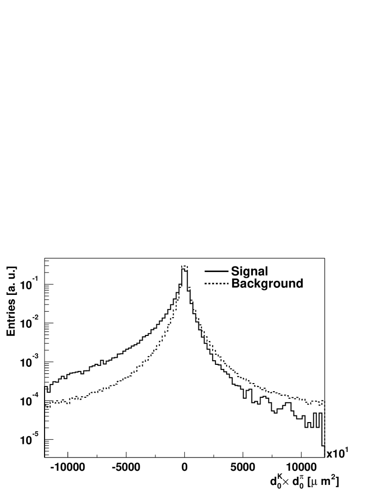
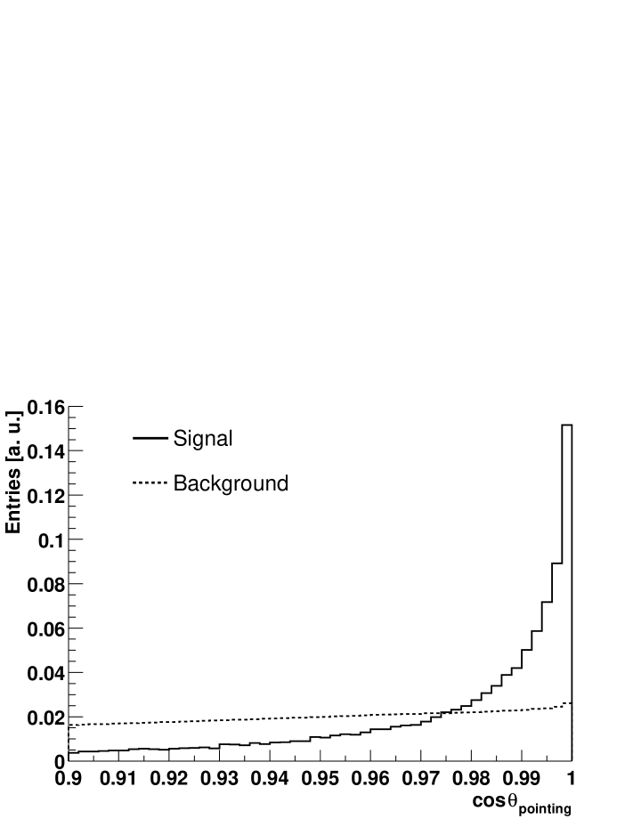
Figure 6.8: Product of the pion and kaon $r\phi$ impact parameters for signal and background combinations. The two distributions are normalized to the same integral.

Figure 6.9: Cosine of the pointing angle for signal and background combinations. The two distributions are normalized to the same integral.

The projection of the tracks on the bending plane allows us to define a sign for the impact parameter. This sign is positive or negative according to the position of the track projection with respect to the primary vertex (the orientation is given by the direction of the track momentum). The tracks of opposite charge originating from a $\mathrm{D^{0}}$ decaying far from the primary vertex will then have impact parameters of opposite signs and large in absolute value. A very appropriate variable for selection is the product of the two transverse projections of the impact parameters. For true decays this quantity should tend to be negative and large in absolute value. In Fig. 6.9 we plot the distribution of the product of impact parameters for signal and background, normalized to the same integral. The cut $d_{0}^{\rm K}\times d_{0}^{\pi}<-40000\leavevmode\nobreak\ \mathrm{\mu m}^{2}$ improves the $S/B$ ratio by a factor $\simeq 10$.

The condition for the $\mathrm{D^{0}}$ to point back to the primary vertex is imposed by a cut on the angle between the momentum vector of the $\mathrm{D^{0}}$ candidate and the line connecting the primary and the secondary vertex (pointing angle $\theta_{\rm pointing}$). The cosine of $\theta_{\rm pointing}$ peaks at $+1$ for the signal, and is almost uniformly distributed for the background, as shown in Fig. 6.9. Requiring to have $\cos\theta_{\rm pointing}>0.98$ would also give, by itself, a background rejection of about one order of magnitude.

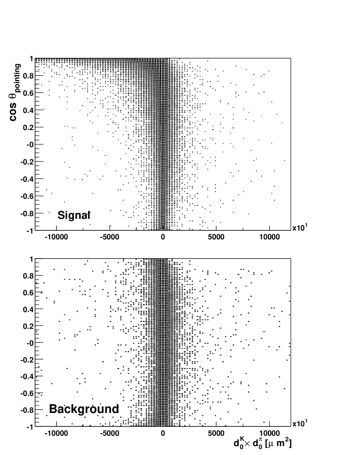
Figure 6.10: Cosine of the pointing angle versus product of the impact parameters for signal and background combinations.

A much larger rejection factor can be obtained by combining these two cuts. In fact, if the secondary vertex is well separated from the primary one, the impact parameters are large and the pointing angle is small, since the $\mathrm{D^{0}}$ flight direction is measured with a better resolution. Therefore, the two variables are strongly correlated in the signal, while this correlation is absent in the background. This can be seen in Fig. 6.10, which shows the bidimensional plot of $\cos\theta_{\rm pointing}$ versus the product of impact parameters. The improvement in the signal-to-background ratio obtained by applying the combined cut is about a factor $10^{3}$.

Each cut was studied in order to maximize the statistical significance $S/\sqrt{S+B}$, calculated for $10^{7}$ central Pb-Pb events. Also, the optimization of the cuts was done separately for the following bins in the $p_{\rm t}$ of the $\mathrm{D^{0}}$: $1<p_{\rm t}<2\ \mathrm{GeV}/c$, $2<p_{\rm t}<3\ \mathrm{GeV}/c$, $3<p_{\rm t}<5\ \mathrm{GeV}/c$, $p_{\rm t}>5\ \mathrm{GeV}/c$. The optimization procedure consists in varying one cut at a time while the others are kept constant and selecting the value of the cut which maximizes the significance. As an example, Fig. 6.11 shows the tuning of the $d_{0}^{\rm K}\times d_{0}^{\pi}$ cut for the different $p_{\rm t}$ bins. The significance is plotted as a function of the value of the cut. For larger momenta the maximum of the significance is found at higher values of the cut, since the impact parameter resolution improves as $p_{\rm t}$ increases.

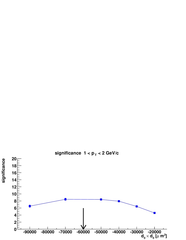
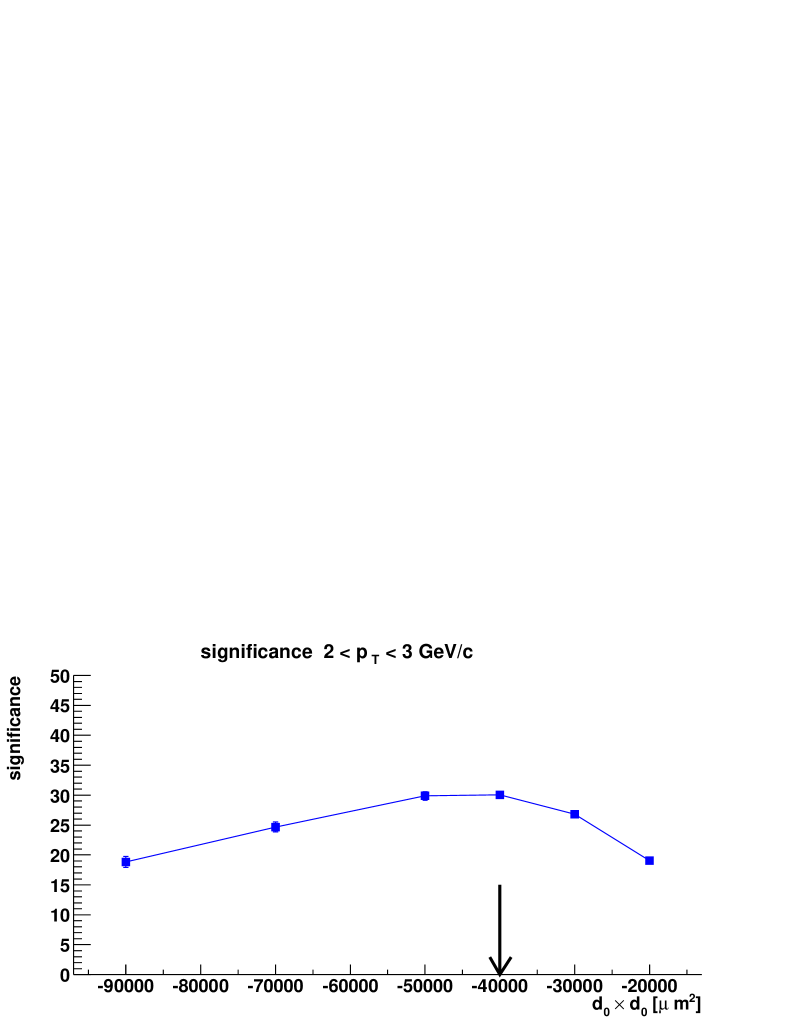
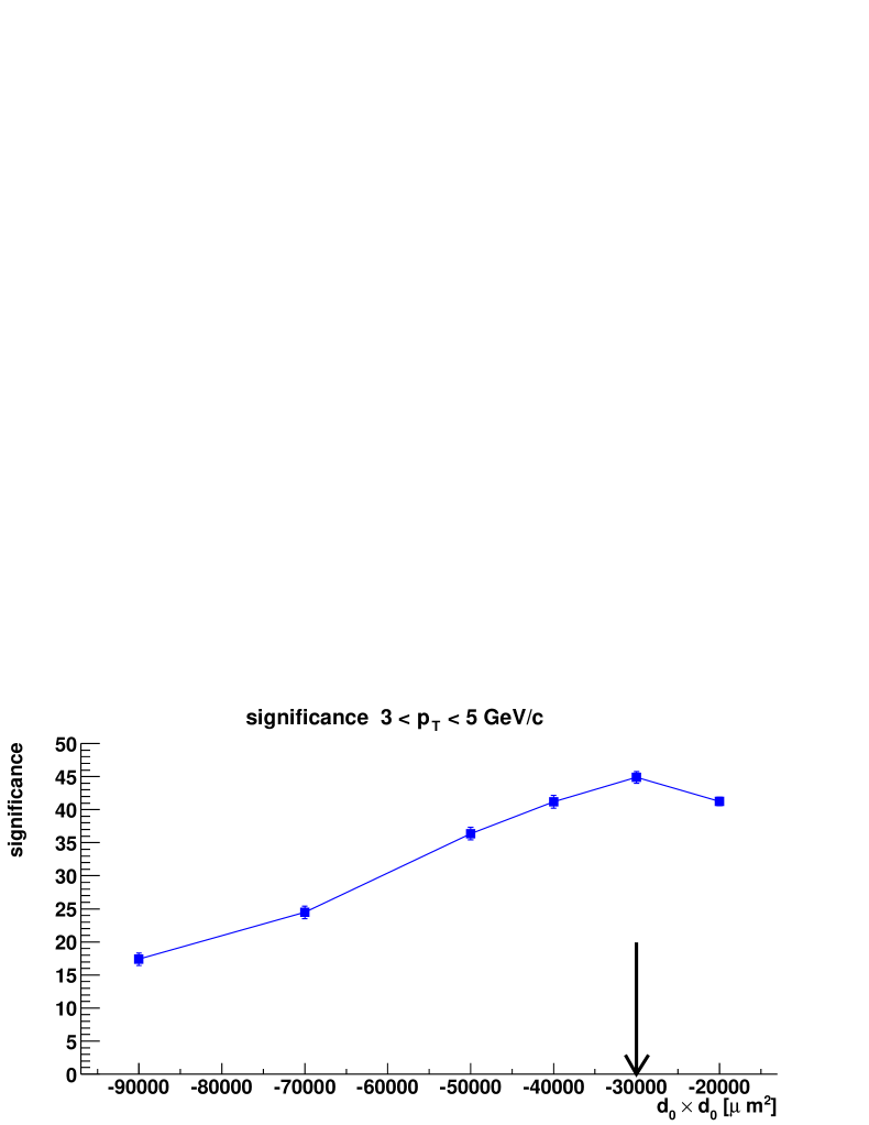
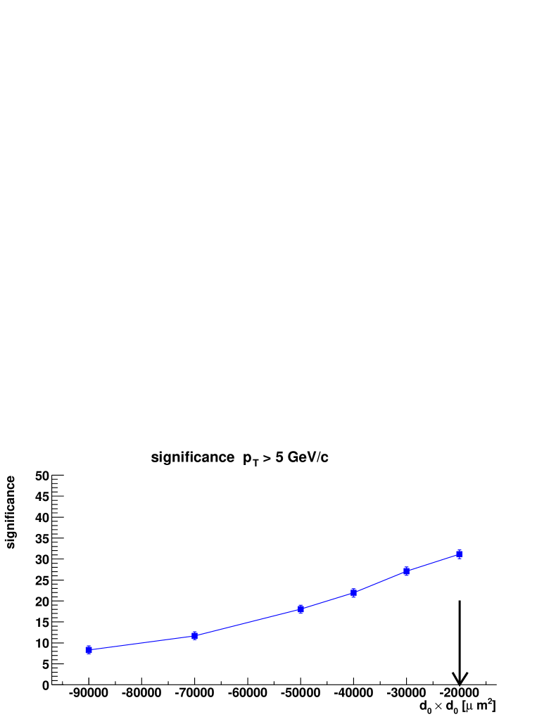
Figure 6.11: Tuning of the $d_{0}^{\rm K}\times d_{0}^{\pi}$ cut for the different $p_{\rm t}^{\rm D^{0}}$ bins. The arrows mark the values chosen for the cut.

Table 6.2: Final value of the cuts in the different $p_{\rm t}$ bins.

Cut name	$1<p_{\rm t}<2\ \mathrm{GeV}/c$	$2<p_{\rm t}<3\ \mathrm{GeV}/c$	$3<p_{\rm t}<5\ \mathrm{GeV}/c$	$p_{\rm t}>5\ \mathrm{GeV}/c$
distance of
closest approach
$(dca)$	$<400\ \mathrm{\mu m}$	$<300\ \mathrm{\mu m}$	$<300\ \mathrm{\mu m}$	$<300\ \mathrm{\mu m}$
decay angle
$|\cos\theta^{\star}|$	$<0.6$	$<0.6$	$<0.6$	$<0.6$
K, $\pi$ $p_{\rm t}$	$>800\leavevmode\nobreak\ \mathrm{MeV}/c$	$>800\leavevmode\nobreak\ \mathrm{MeV}/c$	$>800\leavevmode\nobreak\ \mathrm{MeV}/c$	$>800\leavevmode\nobreak\ \mathrm{MeV}/c$
K, $\pi$ $|d_{0}|$	$<700\ \mathrm{\mu m}$	$<500\ \mathrm{\mu m}$	$<500\ \mathrm{\mu m}$	$<500\ \mathrm{\mu m}$
$\Pi d_{0}=$
$d_{0}^{\rm K}\times d_{0}^{\pi}$	$<-60000\ \mathrm{\mu m}^{2}$	$<-40000\ \mathrm{\mu m}^{2}$	$<-30000\ \mathrm{\mu m}^{2}$	$<-20000\ \mathrm{\mu m}^{2}$
pointing angle
$\cos\theta_{\rm pointing}$	$>0.95$	$>0.98$	$>0.98$	$>0.98$

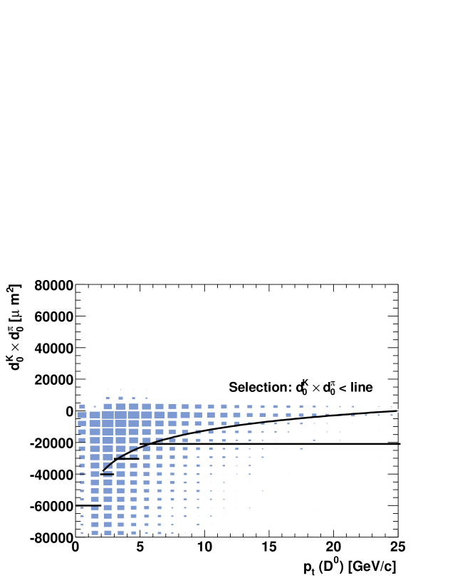
Figure 6.12: Product of the impact parameters as a function of the $\mathrm{D^{0}}$ $p_{\rm t}$ for signal candidates. The step-like cut obtained by the cut-tuning procedure is shown. The line starting from $2\leavevmode\nobreak\ \mathrm{GeV}/c$ represents the smooth cut chosen in order to avoid the loss of signal at high $p_{\rm t}$.

In Table 6.2 the final values of the cuts are reported. The most sensible cut is the one on the product of the impact parameters, since it selects the tail of the distribution in order to exploit the different shapes of signal and background (as shown in Fig. 6.9). Therefore, we studied more carefully the $p_{\rm t}$ dependence of this cut. Figure 6.12 shows the bidimensional plot of $d_{0}^{\rm K}\times d_{0}^{\pi}$ versus $p_{\rm t}^{\rm D^{0}}$ for the signal candidates, after all other cuts have been applied, as reported in Table 6.2. The distribution becomes very narrow at high $p_{\rm t}$ as a consequence of the strong $p_{\rm t}$ dependence of the impact parameter resolution. The step-like cut obtained by the tuning procedure described before is shown. From the shape of the distribution it is clear that using this step-like cut would determine the loss of most of the signal for $p_{\rm t}>8$-$10\leavevmode\nobreak\ \mathrm{GeV}/c$; this high-$p_{\rm t}$ region is extremely important for the parton energy loss studies, as we will see in Chapter 8. It is, therefore, mandatory to have a ‘really’ $p_{\rm t}$-dependent cut, for $p_{\rm t}>2\leavevmode\nobreak\ \mathrm{GeV}/c$, such as the one indicated by the line in the figure.

6.1.5 Results

Figure 6.13 shows the invariant mass distribution for the sum of samples A, B and C after selection, corresponding to $10^{7}$ events.

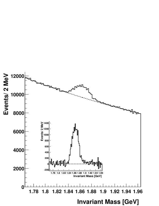
Figure 6.13: $\mbox{$\mathrm{K}$}\pi$ invariant mass distribution for $10^{7}$ events. The same distribution after background subtraction is shown in the inset.

In Table 6.3 the values for $S/$event, $B/$event and $S/B$ , in the invariant mass range $|M_{\rm K\pi}-M_{\rm D^{0}}|<1\leavevmode\nobreak\ \sigma$, are presented. In the same table, we report also the statistical significance $S/\sqrt{S+B}$ for $10^{7}$ central Pb–Pb events and the relative error $\sigma_{S}/S$ on the estimation of the number $S$ of detected $\mathrm{D^{0}}$ mesons. As we shall demonstrate in Chapter 7 this relative error is $\sqrt{S+B}/S$, i.e. the inverse of the significance.

Considering the sum of the three samples A, B and C, the $p_{\rm t}$-integrated significance is 37. Figure 6.14 shows the $p_{\rm t}$ distribution of the signal and of the background absolutely normalized and the significance as a function of $p_{\rm t}$, in bins of $1\leavevmode\nobreak\ \mathrm{GeV}/c$. With $10^{7}$ events the significance is larger than 10 up to about $10\leavevmode\nobreak\ \mathrm{GeV}/c$ of $p_{\rm t}$. For $p_{\rm t}>4\leavevmode\nobreak\ \mathrm{GeV}/c$, the $S/B$ ratio grows but the significance decreases due to the decrease in the signal statistics.

In Fig. 6.15 we show how the signal is distributed in the three PID classes, as a function of the transverse momentum: sample A covers the low-$p_{\rm t}$ region, where the kaon can be efficiently identified in the TOF detector; samples B and C, even if their integrated significances are quite low, are essential to cover the high-$p_{\rm t}$ region above $5\leavevmode\nobreak\ \mathrm{GeV}/c$.

In general, it is convenient to merge the three samples, which essentially corresponds to rejecting only $(\pi_{\rm tag},\,\pi_{\rm tag})$ pairs using the TOF information. However, this strategy gives the quite marginal significance of 8 in the bin $1<p_{\rm t}<2\leavevmode\nobreak\ \mathrm{GeV}/c$. Since for $p_{\rm t}<2\leavevmode\nobreak\ \mathrm{GeV}/c$ sample A contains most of the signal and only a small fraction of the background (see Fig. 6.17), considering only candidates with the kaon identified (sample A) yields a significance of 12 in $1<p_{\rm t}<2\leavevmode\nobreak\ \mathrm{GeV}/c$ (as showed by the star markers in the right panel of Fig. 6.14). Figure 6.17 shows the invariant mass distribution for this sample in $1<p_{\rm t}<2\leavevmode\nobreak\ \mathrm{GeV}/c$; even for this low-$p_{\rm t}$ bin, the signal is well visible over the background.

Table 6.3: Final values of $S/B$ and $S/\sqrt{S+B}$ for $10^{7}$ Pb–Pb events.

Sample	$S/$event	$B/$event	$S/B$	$S/\sqrt{S+B}$ ($10^{7}$ events)	$\sigma_{S}/S$
A	$4.4\cdot 10^{-4}$	$1.4\cdot 10^{-3}$	$32\%$	$33$	$3\%$
B	$4.3\cdot 10^{-4}$	$5.2\cdot 10^{-3}$	$8\%$	$8$	$13\%$
C	$4.6\cdot 10^{-4}$	$5.0\cdot 10^{-3}$	$9\%$	$9$	$11\%$
Total	$1.3\cdot 10^{-3}$	$1.16\cdot 10^{-2}$	$11\%$	$37$	$3\%$

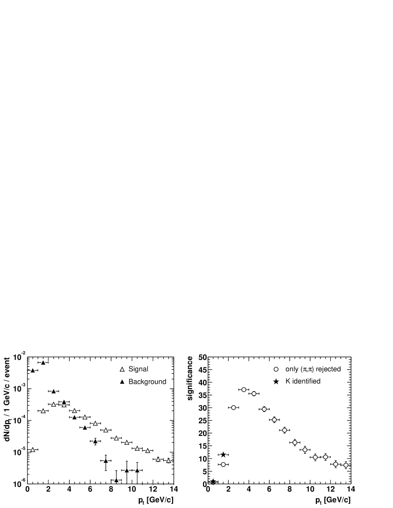
Figure 6.14: Transverse momentum distribution for the signal and for the background after selection (left); the normalization corresponds to 1 central Pb–Pb event. Corresponding significance for $10^{7}$ events as a function of $p_{\rm t}$ (right). The full markers shows the significance obtained for $p_{\rm t}<2\leavevmode\nobreak\ \mathrm{GeV}/c$ requiring the identification of the kaon in the Time of Flight.

Figure 6.15: Transverse momentum distributions for the signal in the three TOF-PID samples.

With the choice of parameters we have used for the generation of the signal, the fraction of the transverse momentum distribution for which we have sensitivity ($p_{\rm t}>1\leavevmode\nobreak\ \mathrm{GeV}/c$) corresponds to about $70\%$ of the total $\mathrm{D^{0}}$ production cross section, at mid-rapidity.

Figure 6.16: Transverse momentum distributions for the signal and for the background after selection for $p_{\rm t}<2\leavevmode\nobreak\ \mathrm{GeV}/c$ (left); the normalization corresponds to 1 central Pb–Pb event. Corresponding significance for $10^{7}$ events as a function of $p_{\rm t}$ (right).

Figure 6.17: $\mbox{$\mathrm{K}$}\pi$ invariant mass distribution in the bin $1<p_{\rm t}<2\leavevmode\nobreak\ \mathrm{GeV}/c$ for the sample of candidates with kaon identified in the Time of Flight ($10^{7}$ events).

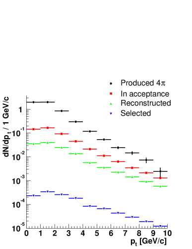
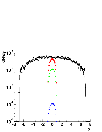
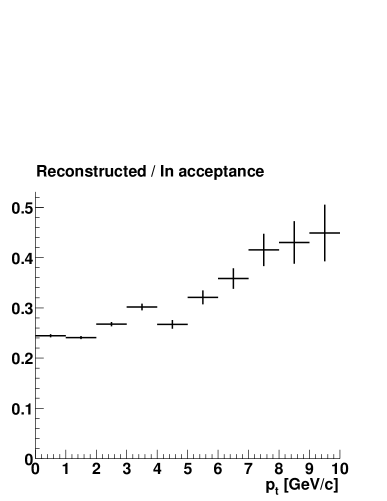
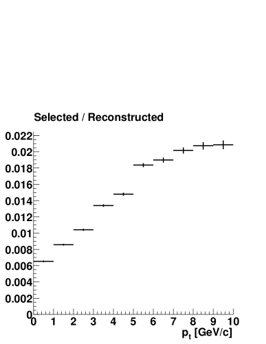
Figure 6.18: In the upper row, transverse momentum and rapidity distributions for the ${\rm D^{0}\to K^{-}\pi^{+}}$ signal: produced per event, with $\mathrm{K}$ and $\pi$ in the acceptance of the barrel ($|\eta|<0.9$), reconstructed and selected. In the lower row: reconstruction and selection efficiencies as a function of $p_{\rm t}$.

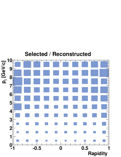
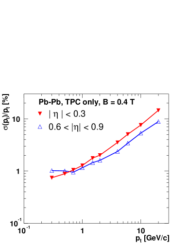
Figure 6.19: Left: selection efficiency as a function of $p_{\rm t}$ and $y$. Right: relative $p_{\rm t}$ resolution in the TPC as a function of $p_{\rm t}$ for tracks in $|\eta|<0.3$ and $0.6<|\eta|<0.9$.

The cuts applied so far, including also the $\pm 1\leavevmode\nobreak\ \sigma$ cut on the invariant mass, reduce the background by a factor $4\cdot 10^{-7}$ and select $\simeq 1\%$ of the signal we had after track reconstruction. In Table 6.4 we summarize the ‘history’ of the signal, showing the effects of acceptance, reconstruction efficiency and selection efficiency. These effects are illustrated as a function of transverse momentum and rapidity in Fig. 6.18. The double-differential plot of the ratio of selected-to-reconstructed $\mathrm{D^{0}}$ as a function of $p_{\rm t}$ and rapidity (Fig. 6.19, left) shows an interesting feature: at a given $p_{\rm t}$, the signal is selected with higher efficiency at the edges of the rapidity acceptance ($|y|\simeq 1$) than in the very central region. This is due to the fact that, at a given $p_{\rm t}$, the $p_{\rm t}$ resolution in the TPC is better for tracks with large $|\eta|$ (Fig. 6.19, right): for these tracks the drift length in the TPC is on average shorter than for tracks close to $\eta=0$ and, therefore, the diffusion effects are smaller and the clusters have better position resolution; only at very low $p_{\rm t}$, where multiple scattering is significant, the resolution is better at small $|\eta|$, because less material is crossed.

Table 6.4: ‘History’ of the $\mbox{$\mathrm{D^{0}}$}/\overline{\mbox{$\mathrm{D^{0}}$}}$ signal in Pb–Pb events.

	$S/$event
Total produced ($4\pi$)	141
Decaying to $\mbox{$\mathrm{K}$}^{\mp}\pi^{\pm}$	5.4
With $\mathrm{K}$ and $\pi$ in $|\eta|<0.9$	0.5
With $\mathrm{K}$ and $\pi$ reconstructed	0.14
After $(\pi_{\rm tag},\,\pi_{\rm tag})$ rejection	0.13
After selection cuts (including $\pm 1\leavevmode\nobreak\ \sigma$ mass cut)	0.0013

6.1.6 Results scaled to a lower-multiplicity scenario

The present analysis assumes a charged particle rapidity density ${\rm d}N_{\rm ch}/{\rm d}y=6000$ for the underlying events. According to recent extrapolations of the RHIC data, the multiplicity is more likely to be of the order of ${\rm d}N_{\rm ch}/{\rm d}y=3000$ (Section 1.4.1). We have therefore estimated how the results on signal-to-background ratio and significance scale in this scenario.

If ${\rm d}N_{\rm ch}/{\rm d}y$ decreases, the number of background pairs decreases as $({\rm d}N_{\rm ch}/{\rm d}y)^{2}$. Therefore, $S/B$ is proportional to $({\rm d}N_{\rm ch}/{\rm d}y)^{-2}$. The significance is proportional to $({\rm d}N_{\rm ch}/{\rm d}y)^{-1}$ if $S\ll B$, so that $S/\sqrt{S+B}\simeq S/\sqrt{B}$. This condition holds for our $p_{\rm t}$-integrated significance, since we have $S\simeq B/10$; for the $p_{\rm t}$-dependent significance such a scaling can be applied only up to $p_{\rm t}\simeq 3\leavevmode\nobreak\ \mathrm{GeV}/c$, as for larger transverse momenta the significance is dominated by the statistics of the signal, $S/\sqrt{S+B}\simeq\sqrt{S}$. In Table 6.5 we just scale the $p_{\rm t}$-integrated results, according to the proportionalities mentioned above, to a case of lower multiplicity. The $\mathrm{c\overline{c}}$ production rate is not rescaled because it is not clear how it is correlated with the total multiplicity and because we have used the average of the values given by the different PDFs, which is already a conservative estimate. In addition, with a lower multiplicity the tracking efficiency would improve and a further improvement can be expected from a refinement of the cuts.

Table 6.5: $S/B$ and $S/\sqrt{S+B}$ as from this analysis (${\rm d}N_{\rm ch}/{\rm d}y=6000$) and scaled for a lower multiplicity (${\rm d}N_{\rm ch}/{\rm d}y=3000$).

${\rm d}N_{\rm ch}/{\rm d}y$	$S/B$	$S/\sqrt{S+B}$ ($10^{7}$ events)
6000	$11\%$	$37$
3000	$44\%$	$74$

6.1.7 Feed-down from beauty

In Section 6.1.1 we pointed out that, for Pb–Pb collisions at $\sqrt{s_{\scriptscriptstyle{{\rm NN}}}}=5.5\leavevmode\nobreak\ \mathrm{TeV}$, about 5% of all the produced $\mathrm{D^{0}}$ mesons come from the decay of B mesons. After the described selections, the ratio of secondary-to-primary $\mathrm{D^{0}}$ increases to $\simeq 12\%$. Such result does not match the expectation that the pointing requirement should suppress the $\mathrm{D^{0}}$ from beauty, as they point to the decay vertex of the B meson and not to the primary vertex. In the following we clarify this picture by analyzing how the main selections affect secondary $\mathrm{D^{0}}$ particles.

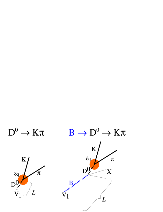
Figure 6.20: Sketch of the decay topologies of primary and secondary $\mathrm{D^{0}}$ mesons. The shaded circle represents the uncertainty $\delta q$ on the reconstructed position of the secondary vertex (see text).

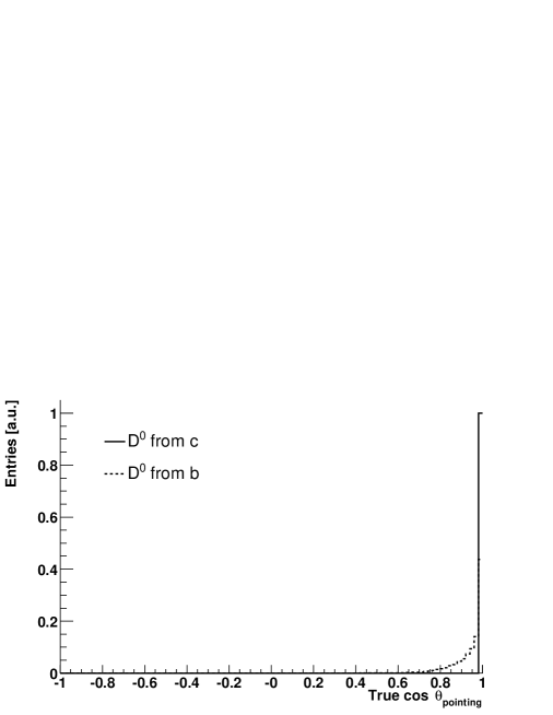
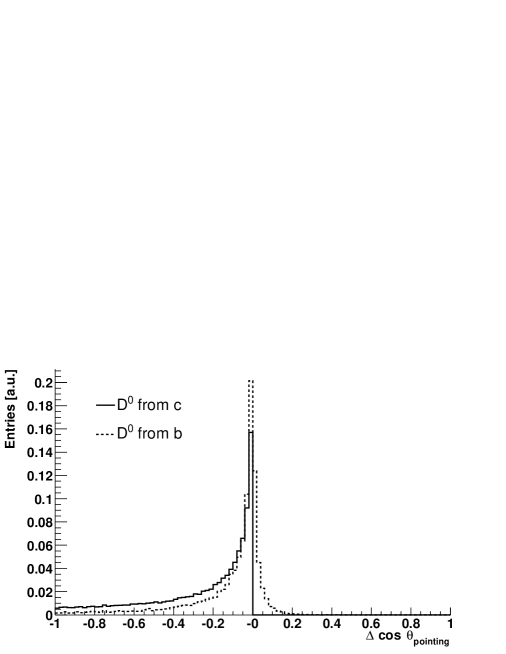
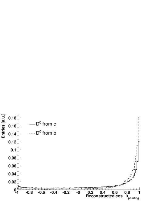
Figure 6.21: Comparison between primary (from c) and secondary (from b) $\mathrm{D^{0}}$ mesons for: true distribution of $\cos\theta_{\rm pointing}$ (top), resolution on $\cos\theta_{\rm pointing}$ (middle) and reconstructed distribution of $\cos\theta_{\rm pointing}$ (bottom). The cut $2<p_{\rm t}<3\leavevmode\nobreak\ \mathrm{GeV}/c$ is applied in order to compare the two signals at the same $p_{\rm t}$.

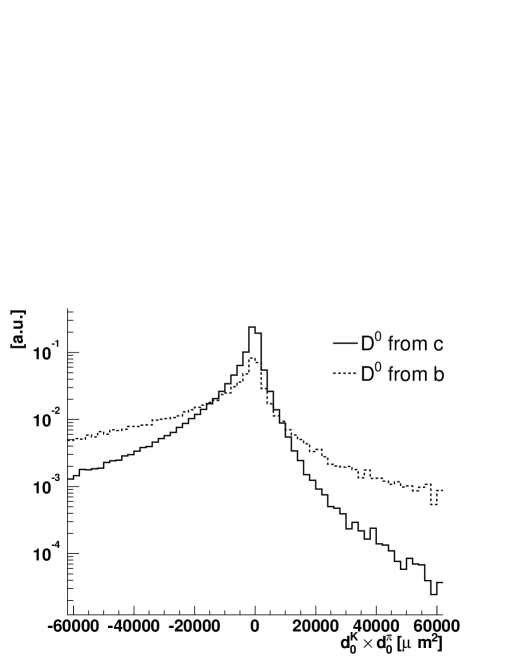
Figure 6.22: Distributions of the product of the impact parameters for primary and secondary $\mathrm{D^{0}}$ mesons (normalized to the same integral).

Figure 6.23: Ratio of secondary-to-primary $\mathrm{D^{0}}$ mesons after track reconstruction and after selections, as a function of $p_{\rm t}$.

Pointing angle:

this cut has the effect to enhance the fraction of secondary $\mathrm{D^{0}}$. In fact, in the decay ${\rm B}\to{\rm D^{0}}+X$, the $\mathrm{D^{0}}$ takes most of the momentum of the B meson and, thus, it approximately follows its flight line. Figure 6.21 (top panel) shows that the ‘true’ distribution of $\cos\theta_{\rm pointing}$ (generator level) for secondary $\mathrm{D^{0}}$ is accumulated in the region $\cos\theta_{\rm pointing}>0.9$. Moreover, the resolution on this variable is better in the case of secondary $\mathrm{D^{0}}$ particles (Fig. 6.21, middle panel, for $2<p_{\rm t}<3\leavevmode\nobreak\ \mathrm{GeV}/c$). This is explained by the sketch in Fig. 6.20: at the same value of $p_{\rm t}$ the resolution $\delta q$ on the position of the secondary vertex is the same for primary and secondary $\mathrm{D^{0}}$ particles, but the resolution on the pointing angle is proportional to $\delta q/L$, where $L$ is the distance of the secondary vertex from the interaction point, which is larger for $\mathrm{D^{0}}$ from B decays. As a consequence, the reconstructed distribution of $\cos\theta_{\rm pointing}$ is more accumulated at 1 for secondary than for primary $\mathrm{D^{0}}$ particles (Fig. 6.21, bottom panel).

Product of the impact parameters:

the tracks from the decay ${\rm B}\to\mbox{${\rm D^{0}\to K^{-}\pi^{+}}$}$ have larger impact parameters than those from ${\rm D^{0}\to K^{-}\pi^{+}}$ and the selection $d_{0}^{\rm K}\times d_{0}^{\pi}<-40000\leavevmode\nobreak\ \mathrm{\mu m}^{2}$ enhances the fraction of the former in the final sample (Fig. 6.23).

Upper cut on $d_{0}$:

the analysis cut $|d_{0}|<500\leavevmode\nobreak\ \mathrm{\mu m}$, introduced to reject the background from strange-particle decays, is effective also to reduce by $\simeq 30\%$ the fraction of $\mathrm{D^{0}}$ from B mesons.

The ratio ($\mathrm{D^{0}}$ from b)/($\mathrm{D^{0}}$ from c) is reported in Fig. 6.23 as a function of $p_{\rm t}$, after track reconstruction and after selections. The ratio grows with $p_{\rm t}$ due to the harder spectrum of the $\mathrm{D^{0}}$ from beauty. The increase in the fraction of secondary $\mathrm{D^{0}}$ after selections is very large at low $p_{\rm t}$ where tighter displaced vertex requirements have to be applied in order to reject the combinatorial background.

6.2 Feasibility study for pp collisions

The study for the detection of ${\rm D^{0}\to K^{-}\pi^{+}}$ decays in pp events followed the same general lines as that for the Pb–Pb case. In particular, the same selection strategy was adopted, with cuts on the product of impact parameters and on the pointing angle.

The significance of the extracted signal should be much higher in pp than in Pb–Pb, because:

1. The detector performance is better in the very-low-multiplicity environment of pp collisions. As an example the tracking efficiency is larger by about 10% (see Fig. 4.6).

2. Without taking into account the improved efficiency, the initial $S/B$ ratio is proportional to $N^{\scriptstyle{\rm c\overline{c}}}/({\rm d}N_{\rm ch}/{\rm d}y)^{2}$; the charm production yield is lower by a factor about 700 in pp with respect to Pb–Pb (see Table 3.5), but the multiplicity of the background event is lower by a factor 1000 ($\left\langle{\rm d}N_{\rm ch}/{\rm d}y\right\rangle=6$ in pp with PYTHIA); therefore, the initial $S/B$ is larger by a factor $\simeq 1500$ in pp collisions.

However, the larger uncertainty on the position of the interaction vertex, extensively discussed in Chapters 4 and 5, is a clear and important disadvantage for the displaced vertex selection in the pp case. In the following, along with the results for the realistic scenario (indicated as “vertex reconstructed”), we present also the results for a scenario of perfect knowledge of the vertex position (“vertex known”). This is done in order to (a) have a situation (“vertex known”) more directly comparable to the Pb–Pb one and (b) quantify and understand the weight of the larger uncertainty on the vertex position.

6.2.1 Background and signal generation

The magnetic field was set to same value as for Pb–Pb, $0.4$ T. The same settings were used also for the generation of the position of the interaction vertex.

Background

Proton–proton minimum-bias events at a centre-of-mass energy $\sqrt{s}=14\leavevmode\nobreak\ \mathrm{TeV}$ were generated using PYTHIA, as described in Section 4.2.1, excluding diffractive topologies. The average charged particle rapidity density is $\left\langle{\rm d}N_{\rm ch}/{\rm d}y\right\rangle=6$. A total of $8.5\cdot 10^{6}$ events were used. These events correspond to $12.1\cdot 10^{6}$ minimum-bias events using $\sigma_{\rm pp}^{\rm non-diffr.}/\sigma_{\rm pp}^{\rm inel}=0.7$ from PYTHIA. Half of the statistics was produced and analyzed using the distributed computing facilities at CERN and in about 10 sites in Europe. Large productions, for a total of $\approx$ 300,000 CPU hours, were managed by means of AliEn [92], the ALICE interface to the grid computing network.

All the results are given for $10^{9}$ pp minimum-bias events, corresponding to a run of 1 month.

Signal

For the generation of the $\mathrm{D^{0}}$ signal we did not use the same method as in the Pb–Pb case, i.e. generating many ${\rm D^{0}\to K^{-}\pi^{+}}$ decays in special signal events. In the case of pp collisions, it is essential to have the signal with ‘its own pp event’ for two main reasons:

1. The primary vertex has to be reconstructed event-by-event using the tracks; therefore, the signal events must be pp events with charm, as we will show that, in PYTHIA, events with charm have different properties, in terms of particle production, with respect to events without charm.

2. In pp, medium- and high-multiplicity events are characterized by the presence of jets of particles emitted in narrow cones in the fragmentation of energetic partons; there might be a significant background originated from the association of one track from the $\mathrm{D^{0}}$ decay with one of the tracks in the same jet.

Therefore, we generated standard pp events with PYTHIA, with the same settings as for the generation of the background, and we selected events that contained a $\mathrm{D^{0}}$ in $|y|<1$ (the decay in the $\mbox{$\mathrm{K}$}\pi$ channel was forced). The part of these $\mathrm{D^{0}}$ mesons coming from beauty feed-down was weighted in order to match the correct ratio secondary/primary (Section 6.1.1). We used $2\cdot 10^{6}$ such events, corresponding to $1.7\cdot 10^{9}$ pp minimum-bias events, using the yields in Table 3.8.

The drawback of this method is that the produced $\mathrm{D^{0}}$ mesons have to be reweighted according to their $p_{\rm t}$ in order to reproduce the distributions given by the NLO pQCD calculations. In fact, the settings of PYTHIA necessary to reproduce these distributions cannot be used to generate standard pp events. The $\mathrm{D^{0}}$ from charm and from beauty were reweighted separately, in order to keep into account their different $p_{\rm t}$ spectra.

Properties of pp events with charm production

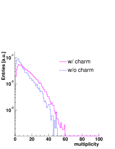
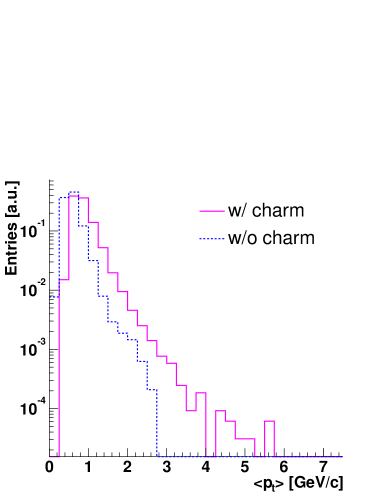
Figure 6.24: Charged multiplicity (left) and mean $p_{\rm t}$ (right) in $|\eta|<0.9$ for PYTHIA events with and without charm production. Histograms are normalized to the same integral.

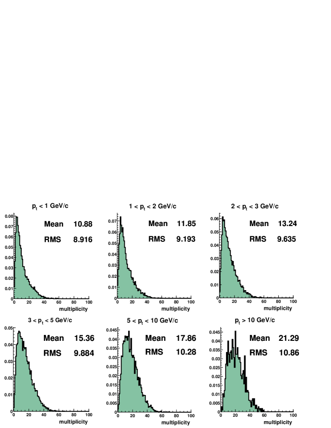
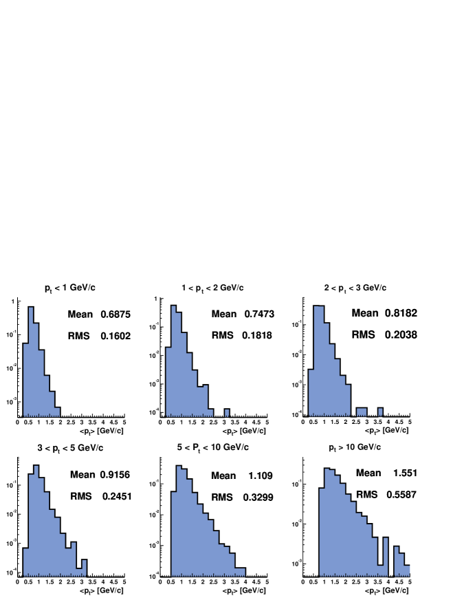
Figure 6.25: Charged multiplicity (top) and mean $p_{\rm t}$ (bottom) in $|\eta|<0.9$ for PYTHIA events with charm production, in bins of $p_{\rm t}$ of a D meson produced in the event.

In Chapter 5 we have shown that the efficiency and resolution for the reconstruction of the primary vertex in pp events depends on the number of produced particles and on their average transverse momentum.

Due to the large mass of heavy quarks, one expects the events with charm (or beauty) to yield more particles than other events, and with larger mean energy. This is a very important aspect, because it would imply that the vertex information is quantitatively better in events containing charm particles.

At lower energies, a difference in the mean multiplicity of events with and without charm was observed by the NA27 Collaboration in pp fixed-target interactions with a beam energy of $400\leavevmode\nobreak\ \mathrm{GeV}$ [93]. The average charged multiplicity was found to be $\left\langle N_{\rm ch}\right\rangle=11$ and $\left\langle N_{\rm ch}\right\rangle=9$ for events with and without charm, respectively. In the former case, two completely reconstructed charm mesons were required; each of them contributed for one unit to the count of the multiplicity and their decay products were not counted.  

Comparing the properties, in terms of multiplicity and mean transverse momentum, of PYTHIA pp events with and without charm production, we found that:

1. Events with charm production have significantly larger multiplicity and mean $p_{\rm t}$.

2. With respect to a D meson produced in the collisions, the quantities $\left\langle\rm multiplicity\right\rangle$ and $\left\langle p_{\rm t}\right\rangle$ increase as the transverse momentum of the D meson increases.

Figure 6.24 (left) presents the distribution of the charged multiplicity in $|\eta|<0.9$ (ALICE barrel acceptance) for events with and without charm (for events with charm we used the same counting rules as in Ref. [93]): the averages are 14 and 10, respectively. The mean $p_{\rm t}$ is shown on the right panel of the same figure: the average values are $850\leavevmode\nobreak\ \mathrm{MeV}/c$ and $600\leavevmode\nobreak\ \mathrm{MeV}/c$, respectively. In Fig. 6.25 the same distributions, for events with charm production, are shown in bins of $p_{\rm t}$ of a D meson produced in the event.

6.2.2 Event reconstruction and particle identification

Track reconstruction was performed in the same way as for the Pb–Pb case, using the parameterization of the tracking response in the TPC, with a pp-specific tuning, and the Kalman filter in the ITS, where at least 5 clusters (2 in the pixel layers) were required.

After the tracking, the interaction vertex position was determined by means of the reconstructed tracks, as described in Section 5.3. In order not to bias the measurement of the impact parameters of the two $\mathrm{D^{0}}$ decay tracks, for each $\mathrm{D^{0}}$ candidate the vertex was reconstructed excluding the two tracks belonging to the candidate.

In the low-multiplicity environment of proton–proton collisions, the particle identification in the Time of Flight is more efficient, because the probability to match incorrectly the tracks with the TOF pads is much lower. In Fig. 6.26 we show the tagging probabilities, defined as for Pb–Pb and obtained by optimizing for pp collisions the graphical cuts applied on the momentum-versus-mass plane. We remark that in this case the contamination of kaons in the pion sample, i.e. the probability to tag a kaon as pion, is almost negligible. Consequently, the fraction of $\mathrm{D^{0}}$ signal lost for this reason goes down to 2% in pp (it is about 10% in Pb–Pb).

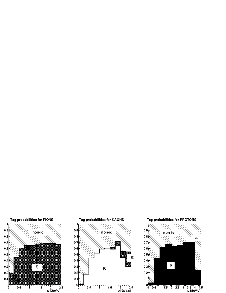
Figure 6.26: PID tag probabilities for reconstructed pions, kaons and protons in pp collisions with the TOF detector.

6.2.3 Analysis and results

Table 6.6: Initial statistics for signal and background (in $M_{\rm D^{0}}\pm 3\leavevmode\nobreak\ \sigma$), for pp and Pb–Pb. Sample A+B+C. The ratio Pb–Pb/pp is also reported.

	$S/$event	$B/$event	$S/B$
pp	$2.4\cdot 10^{-4}$	$1.1\cdot 10^{-1}$	$2.3\cdot 10^{-3}$
Pb–Pb	$1.3\cdot 10^{-1}$	$2.8\cdot 10^{4}$	$4.5\cdot 10^{-6}$
ratio Pb–Pb/pp	520	$2.6\cdot 10^{5}$	$2\cdot 10^{-3}$

The statistics for signal and background after track reconstruction are reported in Table 6.6. Here and in the following we consider the sum of the three samples A, B and C, where not differently specified. Only a $\pm 3\leavevmode\nobreak\ \sigma$ cut on the invariant mass is applied (the invariant mass resolution for the $\mathrm{D^{0}}$ is 10% better in pp than in Pb–Pb, due to the improved momentum resolution). In the table, along with the values for pp, also the same values for Pb–Pb and the ratio between the two are quoted, for comparison purposes. The initial signal-to-background ratio is much larger (about three orders of magnitude) in pp than in Pb–Pb. This is due to the fact that, when going from pp to Pb–Pb, the background, which is combinatorial, increases much more than the signal. It is important to understand in a semi-quantitative way the changes in $S$ and $B$:

• The charm yield increases by a factor 720 from pp to Pb–Pb (Table 3.5), but, as tracking and PID efficiencies are worse in Pb–Pb by $\approx 10\%$ each, this increase is reduced to 520 after tracking and TOF-PID: $720\times(\epsilon_{\rm PID}^{\rm Pb-Pb}/\epsilon_{\rm PID}^{\rm pp})\times(\epsilon_{\rm track}^{\rm Pb-Pb}/\epsilon_{\rm track}^{\rm pp})^{2}=720\times 0.9\times(0.9)^{2}\approx 520$.

• For the background, the average number of reconstructed tracks per event is 4600 for Pb–Pb and 6 for pp; therefore, the increase in the number of track pairs should be $(4600/6)^{2}\approx 5.9\cdot 10^{5}$. The obtained ratio is a factor 2 lower (see Table 6.6); this is due to the fact that in pp the number of reconstructed tracks has large event-by-event fluctuations, and thus the combinatorial background is larger than $\left\langle N_{\rm tracks}\right\rangle^{2}$.

The background with 1 track from a D meson and the other from the underlying event is a negligible fraction (0.1%) of the total background and it is about a factor 2 lower than the signal. We will show in the following that it is almost completely suppressed by the selection cuts.

Selection and results are shown for the case “primary vertex known” first, and then for the more realistic case “primary vertex reconstructed”.

Scenario 1: “primary vertex known”

In this scenario we assume the $(x,y)$ position of the interaction point to be known as precisely as it is in the case of Pb–Pb collisions. The position along $z$ is measured using the reconstructed tracks with a resolution of $\sim 100\leavevmode\nobreak\ \mathrm{\mu m}$. We remark that this might be the case if the machine luminosity is below the nominal value so that beam defocusing or displacements are not necessary at the ALICE IP (see Section 4.3.3). This is likely to happen during the start-up runs at the LHC.

In Fig. 6.27 we report the distributions of the two main variables for the selection, $d_{0}^{\rm K}\times d_{0}^{\pi}$ and $\cos\theta_{\rm pointing}$, for the signal in Pb–Pb and in pp. Both distributions have similar shape in the two cases. This is not surprising for the product of the impact parameters, since it was shown in Chapter 5 that the track position resolution is the same for Pb–Pb and pp events and we are assuming the same resolution on the primary vertex in the bending plane. In the case of the pointing angle one may expect the resolution in pp to be spoiled by the fact that the $z$ position of the primary vertex is known with a resolution of $100\leavevmode\nobreak\ \mathrm{\mu m}$, with respect to $6\leavevmode\nobreak\ \mathrm{\mu m}$ in Pb–Pb. However, this difference does not affect too much the pointing angle resolution, since the dominant contributions to it come from the position resolution of the secondary vertex, which is of $\sim 70\times 70\times 120\leavevmode\nobreak\ \mathrm{\mu m}^{3}$ in the three perpendicular directions for a $\mathrm{D^{0}}$ with $p_{\rm t}\simeq 2\leavevmode\nobreak\ \mathrm{GeV}/c$.

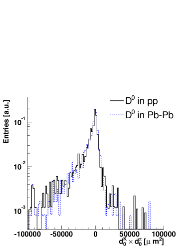
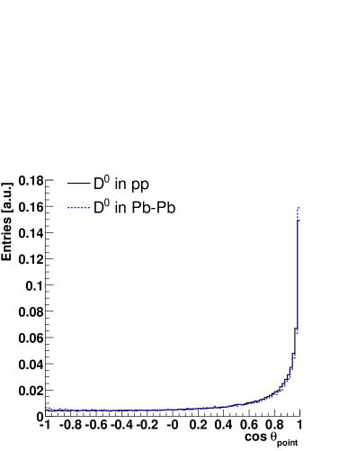
Figure 6.27: Distribution of the product of impact parameters (left) and of the cosine of the pointing angle (right) for $\mathrm{D^{0}}$ mesons in Pb–Pb and pp (case “vertex known”) events.

Table 6.7: Final value of the cuts in the different $p_{\rm t}$ bins for pp (case “vertex known”).

Cut name	$p_{\rm t}<1\leavevmode\nobreak\ \mathrm{GeV}/c$	$1<p_{\rm t}<2\ \mathrm{GeV}/c$	$2<p_{\rm t}<3\ \mathrm{GeV}/c$	$3<p_{\rm t}<5\ \mathrm{GeV}/c$	$p_{\rm t}>5\ \mathrm{GeV}/c$
distance of
closest approach
$(dca)$	$<400\ \mathrm{\mu m}$	$<300\ \mathrm{\mu m}$	$<200\ \mathrm{\mu m}$	$<200\ \mathrm{\mu m}$	$<200\ \mathrm{\mu m}$
decay angle
$|\cos\theta^{\star}|$	$<0.8$	$<0.8$	$<0.8$	$<0.8$	$<0.8$
K, $\pi$ $p_{\rm t}$	$>500\leavevmode\nobreak\ \mathrm{MeV}/c$	$>600\leavevmode\nobreak\ \mathrm{MeV}/c$	$>700\leavevmode\nobreak\ \mathrm{MeV}/c$	$>700\leavevmode\nobreak\ \mathrm{MeV}/c$	$>700\leavevmode\nobreak\ \mathrm{MeV}/c$
K, $\pi$ $|d_{0}|$	$<\infty$	$<\infty$	$<\infty$	$<\infty$	$<\infty$
$\Pi d_{0}=$
$d_{0}^{\rm K}\times d_{0}^{\pi}$	$<-20000\ \mathrm{\mu m}^{2}$	$<-20000\ \mathrm{\mu m}^{2}$	$<-20000\ \mathrm{\mu m}^{2}$	$<-10000\ \mathrm{\mu m}^{2}$	$<-5000\ \mathrm{\mu m}^{2}$
pointing angle
$\cos\theta_{\rm pointing}$	$>0.7$	$>0.7$	$>0.7$	$>0.7$	$>0.7$

The values of the cuts, tuned in order to maximize the significance, in different $p_{\rm t}$ bins, are reported in Table 6.7. We notice that, as a consequence of the better initial $S/B$ ratio, the cuts on impact parameters and pointing angle are much less tight than in the Pb–Pb case. In addition, the cut on the maximum absolute value of $d_{0}$ is not necessary. As in Pb–Pb, a smooth $p_{\rm t}$-dependent cut for the product of the impact parameters was used.

The final statistics are shown in Table 6.8: the integrated $S/B$ ratio is 50% and the significance for $10^{9}$ pp minimum-bias events is 84. The lower $p_{\rm t}$ limit is $\simeq 0$, with a significance of 17 for $0<p_{\rm t}<1\leavevmode\nobreak\ \mathrm{GeV}/c$ if the K identification in the TOF is required.

Table 6.8: Final values of $S/B$ and significance for pp (case “vertex known”). The results for Pb–Pb are reported for comparison.

System	$S/$event	$B/$event	$S/B$	$S/\sqrt{S+B}$	$\sigma_{S}/S$
pp ($10^{9}$ events)	$2.1\cdot 10^{-5}$	$4.1\cdot 10^{-5}$	$50\%$	$84$	$1\%$
Pb–Pb($10^{7}$ events)	$1.3\cdot 10^{-3}$	$1.16\cdot 10^{-2}$	$11\%$	$37$	$3\%$

Scenario 2: “primary vertex reconstructed”

We now consider the scenario in which the information on the vertex position in the transverse plane given by the position and size of the proton beams is very poor ($\sim 150\leavevmode\nobreak\ \mathrm{\mu m}$). Since this uncertainty is larger than the track position resolution given by the pixels and the mean impact parameter of the decay products of $\mathrm{D^{0}}$ mesons is $\sim 100\leavevmode\nobreak\ \mathrm{\mu m}$, it is clear that, without a primary vertex reconstruction, it is impossible to separate the decay vertex from the interaction point. Figure 6.28 shows the distribution of the product of impact parameters ($\Pi d_{0}=d^{\rm K}_{0}\times d_{0}^{\pi}$) in the two cases “vertex known” (labelled $\sigma({\rm vtx})=15\leavevmode\nobreak\ \mathrm{\mu m}$) and “vertex unknown” (labelled $\sigma({\rm vtx})=150\leavevmode\nobreak\ \mathrm{\mu m}$); two $p_{\rm t}$ bins are considered: $1$-$2\leavevmode\nobreak\ \mathrm{GeV}/c$ (left) and $5$-$7\leavevmode\nobreak\ \mathrm{GeV}/c$ (right). In the case “vertex unknown”, at low $p_{\rm t}$ the distributions of signal and background have exactly the same shape and even at high $p_{\rm t}$, where the effect of multiple scattering is negligible, the difference is very tiny.

After the reconstruction of the vertex using the method, specifically developed to this purpose, described in Chapter 5, we obtain the distributions reported in Fig. 6.29. Now a cut at $\Pi d_{0}<-20000\leavevmode\nobreak\ \mathrm{\mu m}^{2}$ allows to improve the $S/B$ ratio even at very low $p_{\rm t}$.

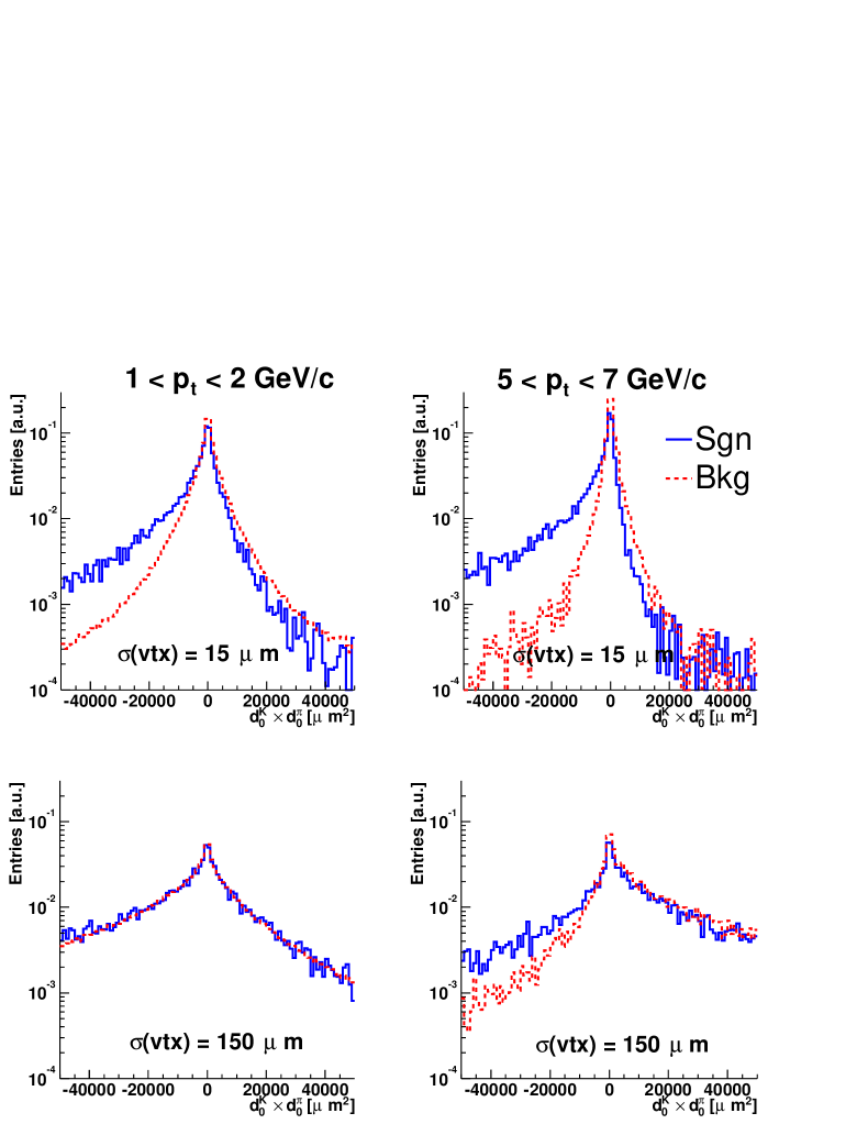
Figure 6.28: Distribution of the product of impact parameters for “vertex known” (top) and “vertex unknown” (bottom).

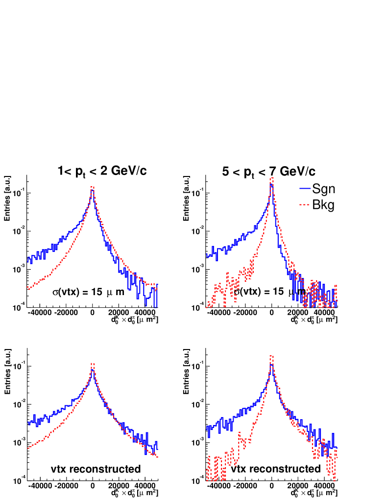
Figure 6.29: Distribution of the product of impact parameters for “vertex known” (top) and “vertex reconstructed” using the tracks (bottom).

By comparing the distributions for the case “vertex reconstructed” (top) to those for the case “vertex known” (bottom) in Fig. 6.29, we notice that, at low $p_{\rm t}$ (left), the distributions of signal and background are both broader, while at higher $p_{\rm t}$ (right) they are almost unchanged. This is, partially, due the fact that a high-$p_{\rm t}$ $\mathrm{D^{0}}$ candidate usually belongs to an event with a relatively high multiplicity, where the vertex is reconstructed more precisely. The other interesting reason is that high-$p_{\rm t}$ $\mathrm{D^{0}}$ candidates are less affected by the uncertainty on the vertex position, in spite of the fact that for high-$p_{\rm t}$ tracks the impact parameter resolution is more affected by this uncertainty than for low-$p_{\rm t}$ tracks (as shown in Fig. 5.15). We explain this point by means of a sketch of a high-$p_{\rm t}$ $\mathrm{D^{0}}$ decay (Fig. 6.30). The two decay tracks form a small angle and the primary vertex lies between them. If we consider the direction $q$ approximately perpendicular to the two tracks, the product of the impact parameters is (see figure):

$$\Pi d_{0}=d_{0}^{\rm K}\times d_{0}^{\pi}\approx(q_{\rm K}-q_{V})\times(q_{\pi}-q_{V}).$$ (6.3)

The error on $\Pi d_{0}$, is function of the errors on the positions of the two tracks, $\sigma(q_{\rm K})$ and $\sigma(q_{\pi})$, and of the error on the primary vertex position, $\sigma(q_{V})$. We obtain:

$$\sigma^{2}(\Pi d_{0})=(d_{0}^{\rm K})^{2}\cdot\sigma^{2}(q_{\pi})+(d_{0}^{\pi})^{2}\cdot\sigma^{2}(q_{\rm K})+(d_{0}^{\rm K}+d_{0}^{\pi})^{2}\cdot\sigma^{2}(q_{V}).$$ (6.4)

The error on the vertex position, in the last term of (6.4), is “weighted” by the square of the sum of the impact parameters. Now, since the impact parameters have preferably opposite signs (as in the example in Fig. 6.30), we have:

$$(d_{0}^{\rm K}+d_{0}^{\pi})^{2}\ll(d_{0}^{\rm K})^{2}\leavevmode\nobreak\ \leavevmode\nobreak\ \leavevmode\nobreak\ \leavevmode\nobreak\ {\rm and}\leavevmode\nobreak\ \leavevmode\nobreak\ \leavevmode\nobreak\ \leavevmode\nobreak\ (d_{0}^{\rm K}+d_{0}^{\pi})^{2}\ll(d_{0}^{\pi})^{2}.$$ (6.5)

Thus, at high-$p_{\rm t}$, the uncertainty on $\Pi d_{0}$ is dominated by the errors on the track positions (first two terms of equation (6.4)) and not by the error on the primary vertex position.

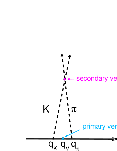
Figure 6.30: Sketch of the decay of a high-$p_{\rm t}$ $\mathrm{D^{0}}$. The impact parameters of the two decay tracks are $q_{\rm K}-q_{V}$ and $q_{\pi}-q_{V}$.

All the cuts were re-optimized and are shown in Table 6.9. Also, the cut $|d_{0}|<500\leavevmode\nobreak\ \mathrm{\mu m}$ used in Pb–Pb was introduced in order to reduce the feed-down from B meson decays (more details on this are given in the next section). The final statistics for the realistic scenario with interaction vertex reconstruction are given in Table 6.10. In the table we have reported as a separate entry the values obtained after applying the additional cut on $|d_{0}|$, in order to point out its effect.

Table 6.9: Final value of the cuts in the different $p_{\rm t}$ bins for pp (case “vertex reconstructed”).

Cut name	$p_{\rm t}<1\leavevmode\nobreak\ \mathrm{GeV}/c$	$1<p_{\rm t}<2\ \mathrm{GeV}/c$	$2<p_{\rm t}<3\ \mathrm{GeV}/c$	$3<p_{\rm t}<5\ \mathrm{GeV}/c$	$p_{\rm t}>5\ \mathrm{GeV}/c$
distance of
closest approach
$(dca)$	$<400\ \mathrm{\mu m}$	$<300\ \mathrm{\mu m}$	$<200\ \mathrm{\mu m}$	$<200\ \mathrm{\mu m}$	$<200\ \mathrm{\mu m}$
decay angle
$|\cos\theta^{\star}|$	$<0.8$	$<0.8$	$<0.8$	$<0.8$	$<0.8$
K, $\pi$ $p_{\rm t}$	$>500\leavevmode\nobreak\ \mathrm{MeV}/c$	$>600\leavevmode\nobreak\ \mathrm{MeV}/c$	$>700\leavevmode\nobreak\ \mathrm{MeV}/c$	$>700\leavevmode\nobreak\ \mathrm{MeV}/c$	$>700\leavevmode\nobreak\ \mathrm{MeV}/c$
K, $\pi$ $|d_{0}|$	$<500\leavevmode\nobreak\ \mathrm{\mu m}$	$<500\leavevmode\nobreak\ \mathrm{\mu m}$	$<500\leavevmode\nobreak\ \mathrm{\mu m}$	$<500\leavevmode\nobreak\ \mathrm{\mu m}$	$<500\leavevmode\nobreak\ \mathrm{\mu m}$
$\Pi d_{0}=$
$d_{0}^{\rm K}\times d_{0}^{\pi}$	$<-20000\ \mathrm{\mu m}^{2}$	$<-20000\ \mathrm{\mu m}^{2}$	$<-20000\ \mathrm{\mu m}^{2}$	$<-10000\ \mathrm{\mu m}^{2}$	$<-5000\ \mathrm{\mu m}^{2}$
pointing angle
$\cos\theta_{\rm pointing}$	$>0.5$	$>0.6$	$>0.8$	$>0.8$	$>0.8$

Table 6.10: Final values of $S/B$ and significance for pp (bold) and Pb–Pb.

System	$S/$event	$B/$event	$S/B$	$S/\sqrt{S+B}$	$\sigma_{S}/S$
pp ($10^{9}$ events)
vertex known	$2.1\cdot 10^{-5}$	$4.1\cdot 10^{-5}$	$50\%$	$84$	$1\%$
pp ($10^{9}$ events)
vertex reconstructed	$1.9\cdot 10^{-5}$	$17.3\cdot 10^{-5}$	$11\%$	$44$	$2\%$
pp (${\bf 10^{9}}$ events)
vertex reconstructed	${\bf 1.5\cdot 10^{-5}}$	${\bf 12.4\cdot 10^{-5}}$	${\bf 12\%}$	${\bf 39}$	${\bf 3\%}$
cut $|d_{0}|<500\leavevmode\nobreak\ \mathrm{\mu m}$
Pb–Pb (${\bf 10^{7}}$ events)	${\bf 1.3\cdot 10^{-3}}$	${\bf 1.16\cdot 10^{-2}}$	${\bf 11\%}$	${\bf 37}$	${\bf 3\%}$

The larger uncertainty on the position of the interaction point in the case “vertex reconstructed” has a quite dramatic effect on the performance for the detection of ${\rm D^{0}\to K^{-}\pi^{+}}$ decays: the background increases by a factor about 4 and, consequently, the $S/B$ ratio and the significance go down by factors 4 and 2, respectively, with respect to the case with small and well-defined interaction region. The additional cut on $|d_{0}|$ reduces the signal by 20% (10% if only sample A is considered for $p_{\rm t}<2\leavevmode\nobreak\ \mathrm{GeV}/c$) and the background by 30%; as we will detail in the next section, is reduces the feed-down from beauty by $30\%$.

In Fig. 6.31 (left) we report the transverse momentum distributions for signal and background. The background with a track from charm, also shown, is negligible. The right panel of the same figure reports the significance as a function of $p_{\rm t}$: as it can be seen, the method developed for the vertex reconstruction allows to maintain the capability of ALICE to measure charm mesons down to essentially 0 in $p_{\rm t}$: the significance is 14 for $0<p_{\rm t}<1\leavevmode\nobreak\ \mathrm{GeV}/c$ if the kaon identification in the TOF is required. For larger transverse momenta, the significances are very close to those obtained in the Pb–Pb case.

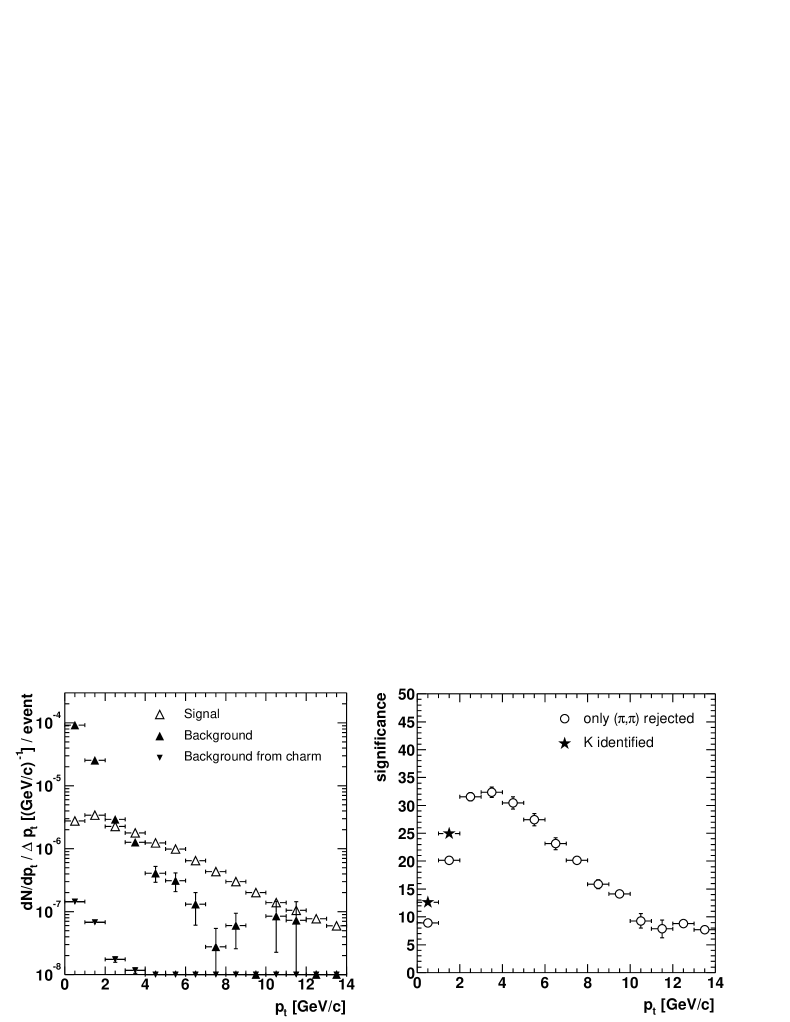
Figure 6.31: Transverse momentum distribution for the signal and for the background after selection (left); the normalization corresponds to 1 pp minimum-bias event. Corresponding significance for $10^{9}$ events as a function of $p_{\rm t}$ (right). The full markers show the significance obtained for $p_{\rm t}<2\leavevmode\nobreak\ \mathrm{GeV}/c$ requiring the identification of the kaon in the Time of Flight.

The ‘history’ of the signal is summarized in Table 6.11. The cuts applied, including a $\pm 1\leavevmode\nobreak\ \sigma$ cut on the invariant mass, select 6% of the signal.

Table 6.11: ‘History’ of the $\mbox{$\mathrm{D^{0}}$}/\overline{\mbox{$\mathrm{D^{0}}$}}$ signal in pp events.

	$S/$event
Total produced ($4\pi$)	0.2
Decaying to $\mbox{$\mathrm{K}$}^{\mp}\pi^{\pm}$	$7.5\cdot 10^{-3}$
With $\mathrm{K}$ and $\pi$ in $|\eta|<0.9$	$7.0\cdot 10^{-4}$
With $\mathrm{K}$ and $\pi$ reconstructed	$2.5\cdot 10^{-4}$
After $(\pi_{\rm tag},\,\pi_{\rm tag})$ rejection	$2.4\cdot 10^{-4}$
After selection cuts (including $\pm 1\leavevmode\nobreak\ \sigma$ mass cut)	$1.5\cdot 10^{-5}$

6.2.4 Feed-down from beauty

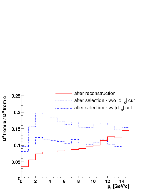
Figure 6.32: Distribution of the pion impact parameter after all selections for primary and secondary $\mathrm{D^{0}}$ mesons. The lines show the cut applied in order to reduce the latter contribution.

Figure 6.33: Ratio of secondary-to-primary $\mathrm{D^{0}}$ mesons after track reconstruction and after selections, as a function of $p_{\rm t}$.

As in the Pb–Pb case, also in pp we observe that the selection cuts have the effect to increase the ratio of secondary-to-primary $\mathrm{D^{0}}$ mesons. The ratio, which is 5.5% after track reconstruction, becomes $\simeq 16\%$ after selections, if we do not apply any cut on the maximum absolute value of the impact parameter, $|d_{0}|$. We remind that the systematic error due to the correction for the feed-down is proportional to this ratio. In order to reduce it, we introduce also for pp the cut $|d_{0}|<500\leavevmode\nobreak\ \mathrm{\mu m}$. Figure 6.33 shows the distribution of $d_{0}^{\pi}$ for the two contributions, after all other selections are applied. The cut, marked by the vertical lines, selects 90% of the $\mathrm{D^{0}}$ from c and 70% of those from b, thus allowing to reduce their ratio from $\simeq 16\%$ to $\simeq 11\%$. The ratio after reconstruction and after selection, without and with the $|d_{0}|$ cut, is reported in Fig. 6.33 as a function of $p_{\rm t}$.

6.3 Expected results for p–Pb collisions

Since the study of the $\mathrm{D^{0}}$ production in pA collisions is a very important tool to disentangle cold- and hot-medium effects in nucleus–nucleus collisions, in particular to investigate nuclear shadowing in the low-$p_{\rm t}$ region (see Section 1.5.2), we give here an estimate of the results for the p–Pb system at $\sqrt{s_{\scriptscriptstyle{{\rm NN}}}}=8.8\leavevmode\nobreak\ \mathrm{TeV}$. We consider minimum-bias collisions, because the precision of a centrality selection for pA collisions is not yet clear.

The average multiplicity given by HIJING for this case, ${\rm d}N_{\rm ch}/{\rm d}y\simeq 20$, is quite close to that obtained for pp with PYTHIA, ${\rm d}N_{\rm ch}/{\rm d}y=6$. Therefore, the detector performance, in terms of tracking and PID, can be assumed to be the same as for proton–proton. For what concerns the interaction vertex, the beams will be focused to the same transverse size as for the Pb–Pb runs, given that p–Pb is a dedicated heavy ion run, optimized for ALICE. On the basis of these considerations, we conclude that a reliable extrapolation can be obtained starting from the results for pp in the scenario with “vertex known”.

In Table 6.12 we report for the charm yield, the multiplicity and the multiplicity squared (which is proportional to the combinatorial background) the values in pp and p–Pb, and the ratio between the two. From pp to p–Pb, the charm yield increases by a factor 4.9, while the multiplicity increases by a factor 3.5.

Table 6.12: Charm yield, multiplicity and square of the multiplicity for pp and p–Pb minimum-bias collisions at LHC energy. The ratio of the values for p–Pb and pp is also reported.

Parameter	pp	p–Pb	p–Pb/pp
$N^{\scriptstyle\mbox{$\mathrm{c\overline{c}}$}}$/event $(\propto S)$	0.16	0.78	4.9
$\left\langle{\rm d}N_{\rm ch}/{\rm d}y\right\rangle$	6	20	3.5
$\left\langle{\rm d}N_{\rm ch}/{\rm d}y\right\rangle^{2}\leavevmode\nobreak\ (\propto B)$	36	400	11

If we assume to use the same values for all the selection cuts as in pp, also the ratios $S_{\rm SELECTED}/S_{\rm INITIAL}$ and $B_{\rm SELECTED}/B_{\rm INITIAL}$ are the same. Thus, $S_{\rm SELECTED}$ and $B_{\rm SELECTED}$ are larger in p–Pb with respect to pp by factors 4.9 and 11, respectively, using Table 6.12.

For the signal-to-background ratio we have:

$${\bf(S/B)_{\rm p-Pb}=}(S/B)_{\rm pp}\times(4.9/11)\simeq 50\%\times 0.5={\bf 25\%}.$$ (6.6)

For the $p_{\rm t}$-integrated significance, keeping into account also that the expected number of collected events is $10^{9}$ for pp and $10^{8}$ for p–Pb:

$$\begin{array}[]{ccl}{\bf(S/\sqrt{S+B})_{\rm p-Pb}}&\simeq&(S/\sqrt{B})_{\rm p-Pb}=(S/\sqrt{B})_{\rm pp}\times 4.9/\sqrt{11}\times\sqrt{10^{8}/10^{9}}\\ &\simeq&84\times 1.5\times\sqrt{0.1}={\bf 40}.\end{array}$$ (6.7)

6.4 Results at lower magnetic field: $B=0.2\leavevmode\nobreak\ {\rm T}$

We pointed out in Chapter 2 that the width of the mass peak of the $\mathrm{D^{0}}$ is proportional to the momentum resolution and, consequently, the integral $B$ of the background under the peak is also proportional to it. As the momentum resolution goes like $1/B_{\rm MAG}$ [60] (we use here the notation $B_{\rm MAG}$ for the magnetic field to distinguish it from the background, $B$), the extrapolation of the results to $B_{\rm MAG}=0.2$ T is straight-forward: the background would be larger by a factor 2.

The $S/B$ ratio would be lower by a factor 2: $\simeq 5\%$ for Pb–Pb and pp, and $\simeq 12\%$ for p–Pb. The $p_{\rm t}$-integrated significance ($\simeq S/\sqrt{B}$) would be lower by a factor $\sqrt{2}$: $\simeq 30$ for Pb–Pb, pp and p–Pb. The low-$p_{\rm t}$ limit would not be much affected: a significance of 10 for the bin $1$-$2\leavevmode\nobreak\ \mathrm{GeV}/c$ in Pb–Pb and for the bin $0$-$1\leavevmode\nobreak\ \mathrm{GeV}/c$ in pp gives a statistical error of 10%, which may still be acceptable. At high-$p_{\rm t}$ the significance does not depend on the magnetic field, since the background is negligible.

6.5 Summary

The results of the feasibility studies for the detection of ${\rm D^{0}\to K^{-}\pi^{+}}$ decays in lead–lead and proton–proton collisions, and the estimated results for proton–lead collisions, are summarized in Table 6.13.

The results are quantitatively comparable for the three considered systems: the $\mathrm{D^{0}}$ production cross section can be measured with a statistical error of the order of 3% (in the next chapter we shall address with more detail the estimation of statistical and systematic errors). In proton–proton, the uncertainty on the interaction vertex position is the main limitation to the performance and a precise vertex reconstruction in three dimensions is a crucial issue.

In terms of performance, the only difference among the three systems is the lower $p_{\rm t}$ limit: $\simeq 1\leavevmode\nobreak\ \mathrm{GeV}/c$ for Pb–Pb and $\simeq 0$ for pp and p–Pb. The upper $p_{\rm t}$ limit is of the order of $15\leavevmode\nobreak\ \mathrm{GeV}/c$, assuming the $p_{\rm t}$ distributions predicted by our baseline NLO pQCD estimates.

If the multiplicity in Pb–Pb collisions at the LHC turns out to match the value extrapolated from RHIC energies (${\rm d}N_{\rm ch}/{\rm d}y\sim 3000$), the expected significance for this system will be larger by a factor 2.

In the previous section, we have shown that, if the lower-field option (0.2 T) was chosen, the results are not expected to change qualitatively, as the lower and upper $p_{\rm t}$ limits are not dramatically affected.

Table 6.13: Summary table of the expected results for ${\rm D^{0}\to K^{-}\pi^{+}}$ detection in pp and Pb–Pb collisions and extrapolated results for p–Pb collisions (using the same cuts as in pp).

System	pp	p–Pb	Pb–Pb
Centrality	min.-bias	min.-bias	central (5% $\sigma^{\rm tot}$)
$\sqrt{s_{\scriptscriptstyle{{\rm NN}}}}$	$14\leavevmode\nobreak\ \mathrm{TeV}$	$8.8\leavevmode\nobreak\ \mathrm{TeV}$	$5.5\leavevmode\nobreak\ \mathrm{TeV}$
Number of events	$10^{9}$	$10^{8}$	$10^{7}$
$S$ (total)	15,000	7,500	13,000
$S/B$	12%	25%	11%
$S/\sqrt{S+B}$	39	40	37
Lower $p_{\rm t}$ limit	$\simeq 0$	$\simeq 0$	$\simeq 1\leavevmode\nobreak\ \mathrm{GeV}/c$
Upper $p_{\rm t}$ limit	$\simeq 15\leavevmode\nobreak\ \mathrm{GeV}/c$	$\simeq 15\leavevmode\nobreak\ \mathrm{GeV}/c$	$\simeq 15\leavevmode\nobreak\ \mathrm{GeV}/c$

Chapter 7 Performance for the measurement of $\mathrm{D^{0}}$ production

The results of the feasibility study presented in Chapter 6 are here used to derive an estimate of the sensitivity for the measurement of the $\mathrm{D^{0}}$ production cross sections and of the transverse momentum distributions in Pb–Pb and pp collisions. Statistical errors are estimated in Section 7.1 and the main systematic uncertainties are discussed in Section 7.2. Eventually, errors are combined and the expected sensitivity is compared, for the pp case, to the theoretical uncertainty in pQCD calculations (Sections 7.3 and 7.4). The extrapolation of the pp results from $\sqrt{s}=14\leavevmode\nobreak\ \mathrm{TeV}$ to $\sqrt{s}=5.5\leavevmode\nobreak\ \mathrm{TeV}$, required to compute the nuclear modification factor $R_{\rm AA}$, is discussed in Section 7.5.

In the last part of the chapter we present a preliminary study on the possibility to separate primary (from c) and secondary (from b) $\mathrm{D^{0}}$ mesons by means of the impact parameter of the $\mathrm{D^{0}}$ itself to the interaction vertex (Section 7.6). Such analysis would be of great interest in order to directly estimate the amount of feed-down from B decays.

7.1 Estimation of the statistical uncertainty

The relative statistical error, $\sigma_{S}/S$, on the number of reconstructed $\mathrm{D^{0}}$ candidates, in a given $p_{\rm t}$-bin and for a given number of events, is equal, as we demonstrate in the following, to the inverse $\sqrt{S+B}/S$ of the statistical significance.

The signal $S$ is obtained as $S=T-B$, where $T$ is the total number ($T=S+B$) of candidates in an invariant mass window entirely containing the $\mathrm{D^{0}}$ peak (e.g. $|M-M_{\rm D^{0}}|<4\leavevmode\nobreak\ \sigma\approx 40$-$60\leavevmode\nobreak\ \mathrm{MeV}$) and $B$ is the number of background candidates in the same window, estimated using, for example, a fit on the side-bands of the invariant mass distribution ($4\leavevmode\nobreak\ \sigma<|M-M_{\rm D^{0}}|<10\leavevmode\nobreak\ \sigma\approx 100$-$200\leavevmode\nobreak\ \mathrm{MeV}$). The error on $S$ is, therefore,

$$\sigma_{S}=\sqrt{\sigma_{T}^{2}+\sigma_{B}^{2}}\approx\sigma_{T}=\sqrt{T}=\sqrt{S+B}.$$ (7.1)

The error on $B$, $\sigma_{B}$, can be neglected; it is, in fact, much lower than the error on $T$, $\sigma_{T}$, since $B$ is estimated on a larger invariant mass range and, thus, with better precision. From Eq. (7.1) we derive trivially $\sigma_{S}/S=1/{\rm significance}$.

In the next section we optimize the $p_{\rm t}$-binning in order to have a significance larger than 10, i.e. statistical error lower than 10%, up to $14\leavevmode\nobreak\ \mathrm{GeV}/c$ and we calculate $S/B$ and significance as a function of $p_{\rm t}$. In Section 7.1.2 we test the expression derived above for $\sigma_{S}/S$ by a fit of Monte Carlo invariant mass distributions.

7.1.1 $S/B$ and $S/\sqrt{S+B}$ with optimized $p_{\rm t}$-binning

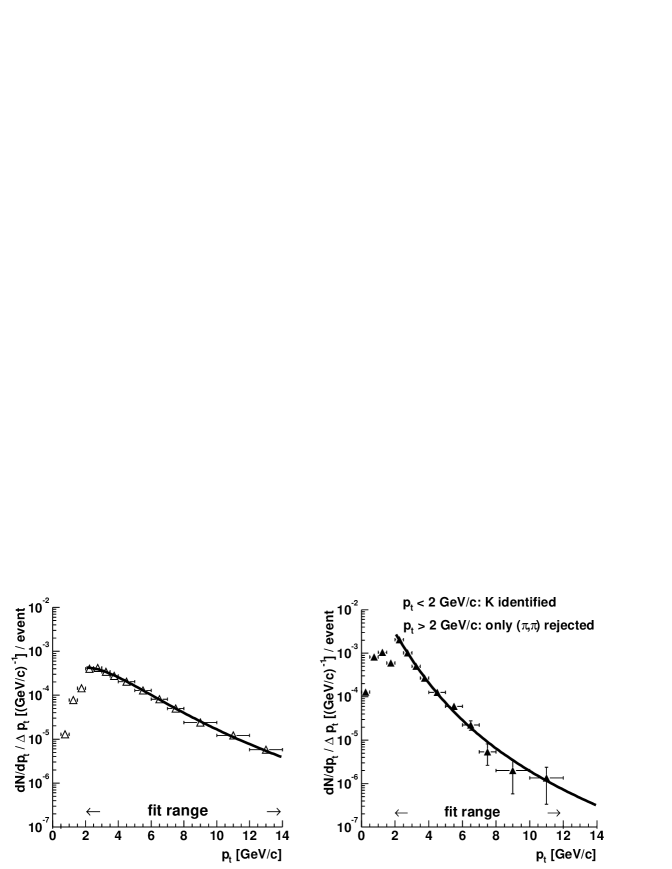
Figure 7.1: Transverse momentum distribution for the signal (left) and for the background (right) in Pb–Pb collisions. The fit in the indicated ranges is performed using the expression introduced in Eq. (3.18).

We fitted the reconstructed $p_{\rm t}$ distributions for signal and background, presented in Figs. 6.14 and 6.31, in order to remove the large fluctuations at high $p_{\rm t}$ due to the limited statistics of the background in the simulations. The fit is shown, for the Pb–Pb case, in Fig. 7.1.

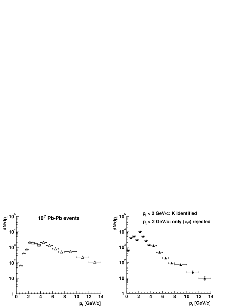
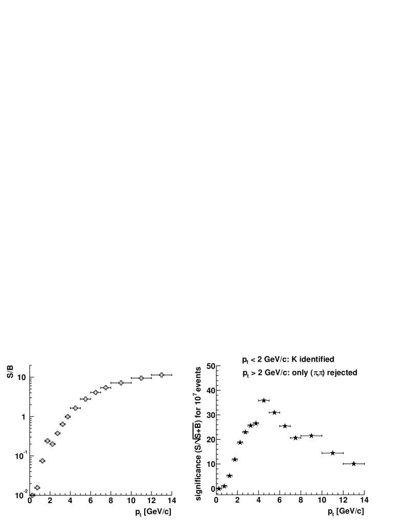
Figure 7.2: Statistics as a function of $p_{\rm t}$ for signal (top-left) and background (top-right) in $|M-M_{\rm D^{0}}|<1\leavevmode\nobreak\ \sigma$, for $10^{7}$ Pb–Pb events. $S/B$ ratio (bottom-left) and significance (bottom-right).

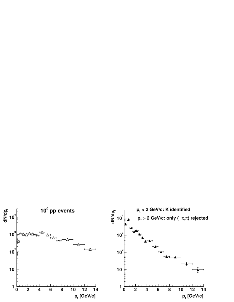
Figure 7.3: Statistics as a function of $p_{\rm t}$ for signal (top-left) and background (top-right) in $|M-M_{\rm D^{0}}|<1\leavevmode\nobreak\ \sigma$, for $10^{9}$ pp events. $S/B$ ratio (bottom-left) and significance (bottom-right).

At high $p_{\rm t}$ the background is negligible and the statistical error is determined by the statistics of the signal: $\sigma_{S}/S\simeq 1/\sqrt{S}$. In order to compensate the decrease in signal statistics, the width of the $p_{\rm t}$-bins is usually increased as $p_{\rm t}$ increases. We chose the following binning:

• $0<p_{\rm t}<4\leavevmode\nobreak\ \mathrm{GeV}/c$: 8 bins with width $\Delta p_{\rm t}=0.5\leavevmode\nobreak\ \mathrm{GeV}/c$;

• $4<p_{\rm t}<8\leavevmode\nobreak\ \mathrm{GeV}/c$: 4 bins with width $\Delta p_{\rm t}=1\leavevmode\nobreak\ \mathrm{GeV}/c$;

• $8<p_{\rm t}<14\leavevmode\nobreak\ \mathrm{GeV}/c$: 3 bins with width $\Delta p_{\rm t}=2\leavevmode\nobreak\ \mathrm{GeV}/c$.

The total statistics for signal and background, the signal-to-background ratio and the significance obtained with this binning are presented in Fig. 7.2 for Pb–Pb ($10^{7}$ events) and in Fig. 7.3 for pp ($10^{9}$ events). The invariant mass window $|M-M_{\rm D^{0}}|<1\leavevmode\nobreak\ \sigma$ is considered. The $p_{\rm t}$ distributions were not divided by the bin width in order to directly show the expected number of signal $\mathrm{D^{0}}$ in each bin.

In both cases, Pb–Pb and pp, the number of selected candidates is of order $\sim 10^{3}$/bin for $p_{\rm t}<8$-$10\leavevmode\nobreak\ \mathrm{GeV}/c$ and of order $\sim 10^{2}$/bin for larger $p_{\rm t}$, up to $14\leavevmode\nobreak\ \mathrm{GeV}/c$. The $S/B$ ratio increases with $p_{\rm t}$ and the significance is larger than 10 (i.e. $\sigma_{S}/S<10\%$) up to $14\leavevmode\nobreak\ \mathrm{GeV}/c$. We consider here $14\leavevmode\nobreak\ \mathrm{GeV}/c$ as the upper $p_{\rm t}$ limit, but we remark that such limit can probably be extended to $17$-$18\leavevmode\nobreak\ \mathrm{GeV}/c$ with one or two more bins of $\Delta p_{\rm t}=2$-$3\leavevmode\nobreak\ \mathrm{GeV}/c$.

7.1.2 Fit of the invariant mass distribution

Before showing the distribution of the relative statistical errors as a function of $p_{\rm t}$, we report the results of a test on the fit of the invariant mass distribution. The test was meant to check:

1. the relation $\sigma_{S}/S=\sqrt{S+B}/S$;

2. the reliability of the statistical error on $S$ given by standard fit algorithms (CERNLIB MINUIT package [94]);

3. that the determination of $S$ by means of a fit does not introduce systematic errors (systematic underestimation or overestimation of $S$).

The ‘true’ shape (without statistical fluctuations) of the invariant mass distribution in $|M-M_{\rm D^{0}}|<200\leavevmode\nobreak\ \mathrm{MeV}/c$ was parameterized, for each $p_{\rm t}$-bin, as an exponential (background) plus a Gaussian (signal). The slope of the exponential and the width of the Gaussian were obtained, as a function of $p_{\rm t}$, from the full simulation; the signal and background contributions were normalized in order to have integrals in $|M-M_{\rm D^{0}}|<1\leavevmode\nobreak\ \sigma$ according to the values reported in the top panels of Figs. 7.2 and 7.3.

From the ‘true’ invariant mass distribution an histogram (with a 5 MeV bin width) was filled and statistical fluctuations were generated by smearing the content of each bin according to a Poisson distribution. The histogram was then fitted to the expression

$$f(M)=\frac{P_{1}(P_{0}-P_{2})}{\exp(-P_{1}M_{\rm min})-\exp(-P_{1}M_{\rm max})}\exp(-P_{1}M)+\frac{P_{2}}{\sqrt{2\pi}P_{4}}\exp\left[-\frac{(M-P_{3})^{2}}{2P_{4}^{2}}\right],$$ (7.2)

where $[M_{\rm min},M_{\rm max}]$ is the fit range, $P_{0}$ is the integral of the distribution in the fit range, which is known (sum of bin contents) and fixed, $P_{1}$ is the slope of the exponential background and $P_{2}$, $P_{3}$, $P_{4}$ are, respectively, the integral ($S$), the mean and the $\sigma$ of the Gaussian that represents the signal. The fit was performed in two steps: (1) fit of the side-bands with an exponential to determine a first approximation of the slope parameter, $P_{1}$; (2) fit of the whole distribution to determine $P_{1}$ and the three parameters of the Gaussian together. Examples of fitted invariant mass distributions for different $p_{\rm t}$-bins in pp collisions are shown in Fig. 7.4.

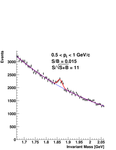
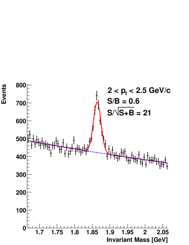
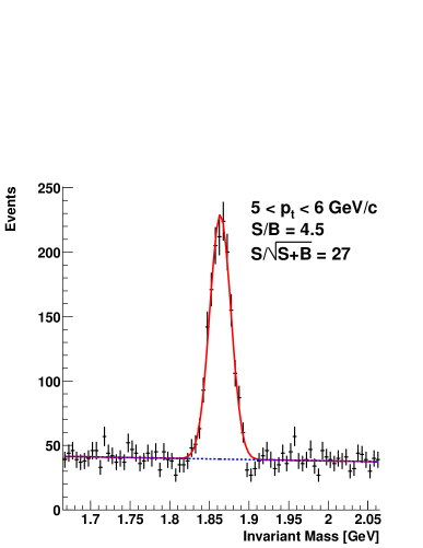
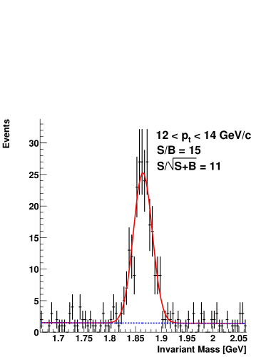
Figure 7.4: Invariant mass distributions in proton–proton collisions fitted to an exponential plus a Gaussian. The statistics correspond to $10^{9}$ pp events.

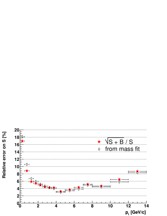
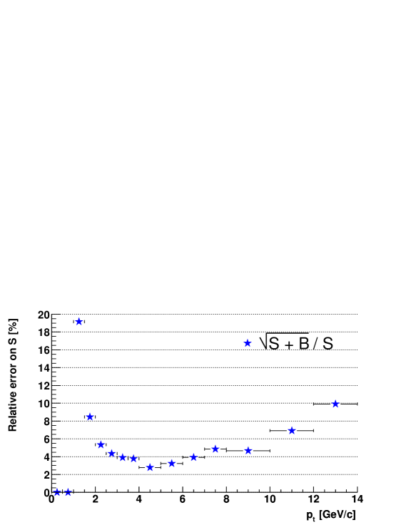
Figure 7.5: Relative statistical errors estimated using the fit test and as the inverse of the significance for $10^{9}$ pp events (top). Relative statistical errors as the inverse of the significance for $10^{7}$ central Pb–Pb events (bottom); for $p_{\rm t}<1\leavevmode\nobreak\ \mathrm{GeV}/c$ the error is larger than 50% and was put to 0 only for graphical representation; these first two bins are not considered in the following analyses.

The procedure of smearing of the histogram bin contents and fit was iterated 1,000 times for each of the 15 $p_{\rm t}$-bins. For a given bin the distribution of the 1,000 residuals of the signal integral, $P_{2}^{\rm fit}-P_{2}^{\rm true}$, is gaussian and its sigma gives the statistical error on $S$. We report in Fig. 7.5 (top panel) the relative statistical errors $\sigma_{S}/S$ for pp as obtained from the described fit test, compared to the expected values, $\sqrt{S+B}/S$: the agreement is satisfactory. We use, therefore, the inverse of the significance as relative statistical error. In the bottom panel of the same figure we show this error for the Pb–Pb case.

The relative statistical error is larger at low $p_{\rm t}$ ($\simeq 20\%$ at $p_{\rm t}\simeq 0$-$0.5\leavevmode\nobreak\ \mathrm{GeV}/c$ in pp and at $p_{\rm t}\simeq 1\leavevmode\nobreak\ \mathrm{GeV}/c$ in Pb–Pb), where the background accumulates; then it goes down to $\simeq 3\%$ at $\simeq 4\leavevmode\nobreak\ \mathrm{GeV}/c$ and it increases again at high $p_{\rm t}$, where the signal statistics decreases.

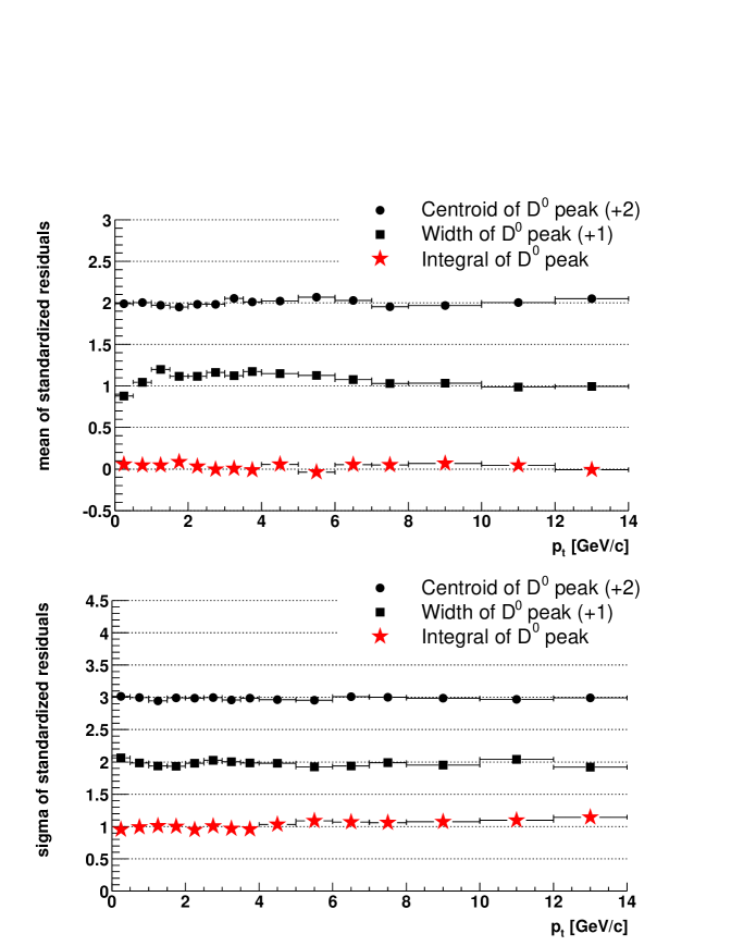
Figure 7.6: Means (top) and sigmas (bottom) of the distributions of the standardized residuals for the three parameters of the invariant mass distribution that describe the signal peak. The case of pp collisions is considered.

The fit algorithm gives also an estimate of the errors, $\delta P_{i}$ for $i=1,2,3,4$, on the 4 parameters, based on the statistical errors on the bin contents of the invariant mass distribution (these errors are visible in Fig. 7.4). From the 1,000 iterations we can study the distributions of the standardized residuals, already introduced in Chapter 5, and defined as $(P_{i}^{\rm fit}-P_{i}^{\rm true})/\delta P_{i}$. If the fit does not introduce systematic shifts in the estimate of the parameters and if the errors given by the fit, $\delta P_{i}$, estimate correctly the statistical errors on the parameters, the distributions of the standardized residuals should be Gaussians with mean equal to 0 (no systematic shift) and $\sigma$ equal to 1 (correct error estimation). Figure 7.6 shows, for pp, the means (top) and the sigmas (bottom) of the distributions of the standardized residuals for the parameters $P_{2}$ (integral of the $\mathrm{D^{0}}$ peak), $P_{3}$ (centroid of the $\mathrm{D^{0}}$ peak) and $P_{4}$ (width of the $\mathrm{D^{0}}$ peak). Over the whole transverse momentum range the means are 0 and the sigmas are 1; we can, therefore, conclude that it is possible to extract the number of selected signal $\mathrm{D^{0}}$ candidates, and its statistical error, by means of a fit on the invariant mass distribution, without introducing additional systematic errors.

7.2 Estimation of systematic uncertainties

The number $S$ of selected signal $\mathrm{D^{0}}$, estimated from the fit, will have to be corrected for efficiency and acceptance in order to obtain the total and $p_{\rm t}$-differential yields, or the cross sections, for $\mathrm{D^{0}}$ production per event. A number of corrections are applied and, in principle, each of them introduces a systematic error. A correction consists, essentially, in multiplying $S$ by a certain factor: $S({\rm corrected})=C\times S($non-corrected$)$; the systematic error introduced is $\delta C\times S($non-corrected$)$, where $\delta C$ is the error on the correction factor $C$. In Table 7.1 we list the main corrections and the expected systematic errors that are introduced.

Table 7.1: Main corrections and related systematic errors.

	Correction	Systematic error
1)	Extrapolation from TOF PID	Matching and PID efficiencies
	to perfect PID	and contaminations in the TOF
2)	Feed-down from beauty	Uncertainty on $\mathrm{b\overline{b}}$ production at LHC
3)	Reconstruction efficiency	Tracking efficiencies and resolutions
4)	Acceptance	Geometrical detector acceptance
5)	From ${\rm D^{0}\to K^{-}\pi^{+}}$ to $\mbox{$\mathrm{D^{0}}$}\to X$	Error on branching ratio ${\rm D^{0}\to K^{-}\pi^{+}}$
6)	Cross section normalization	Pb–Pb: error on centrality selection
		and number of binary collisions
		pp: error on inelastic cross section

The corrections for tracking and PID efficiency and for acceptance are usually done by means of the Monte Carlo simulation of detector geometry and response. The non-perfect description in the simulation of the geometry and of the physics processes that determine the detector response introduces systematic uncertainties (entries 1, 3 and 4 in Table 7.1). It is reasonable to assume that these uncertainties will initially amount to about 10%. However, we remark that experience from other experiments tells that this kind of systematic error can be reduced after few years of running as the understanding of the detector response improves.

The error on the branching ratio of the $\mathrm{D^{0}}$ to the ${\rm K^{-}}\pi^{+}$ channel (entry 5 in Table 7.1) is quite small, 2.4% [60], and it is essentially negligible with respect to the errors from other sources. However, it is included for completeness.

The other errors listed in the table are considered in the next paragraphs.

7.2.1 Correction for feed-down from beauty

After the selection described in Chapter 6, the number of $\mathrm{D^{0}}$ from c quarks will be determined as $N({\rm c\to D^{0}})=N(\mbox{$\mathrm{D^{0}}$})-N({\rm b\to B\to D^{0}})$, where $N(\mbox{$\mathrm{D^{0}}$})$ is the total number of selected $\mathrm{D^{0}}$ and $N({\rm b\to B\to D^{0}})$ is the amount of feed-down from beauty, that will be estimated via Monte Carlo.

The systematic error introduced by this correction is equal to the error on the estimated number of $\mathrm{D^{0}}$ mesons from beauty that pass the selection cuts, $N({\rm b\to B\to D^{0}})$. The relative error on $N({\rm b\to B\to D^{0}})$ is essentially equal to the relative error on the $\mathrm{b\overline{b}}$ production cross section, $\sigma^{\scriptstyle{\rm b\overline{b}}}$, at LHC energy and, thus, the relative error on $N({\rm c\to D^{0}})$ is equal to the relative error on $\sigma^{\scriptstyle{\rm b\overline{b}}}$ multiplied by the ratio of secondary to primary $\mathrm{D^{0}}$, after selections. Such ratio, as obtained with the present baseline on charm and beauty production, has been shown in Figs. 6.23 and 6.33, for Pb–Pb and pp respectively, and it amounts to about 10% on average. At present, the $\mathrm{b\overline{b}}$ cross section at LHC energies is estimated by pQCD calculations at NLO with a very large theoretical uncertainty, $\simeq 80\%$, as we have reported in Chapter 3. We assume here this large relative error. This is probably an overestimate, since B meson production will be measured by ALICE, in the semi-electronic decay channel [95], and also by ATLAS and CMS. However, it is not yet clear how precise these measurements can be, especially at low $p_{\rm t}$.

Multiplying the two factors, 10% (ratio of selected secondary to primary $\mathrm{D^{0}}$) and 80% (relative uncertainty on $\sigma^{\scriptstyle{\rm b\overline{b}}}$), we obtain an average relative error arising from the correction for beauty feed-down of about 8%. We report in Fig. 7.7 this relative error as a function of $p_{\rm t}$ for Pb–Pb (top) and for pp (bottom). The error has different trends as a function of $p_{\rm t}$ in the two cases because different selection cuts are applied in Pb–Pb and in pp.

Recently, the CDF Collaboration has directly estimated the fraction of primary $\mathrm{D^{0}}$ using the distance of the reconstructed $\mathrm{D^{0}}$ flight line to the interaction vertex as a variable to separate primary and secondary $\mathrm{D^{0}}$ [96]. This technique allows them to correct for the feed-down with a systematic error as low as $3$-$5\%$. A preliminary study on the possibility to use the same technique in ALICE was carried out and will be described at the end of this chapter.

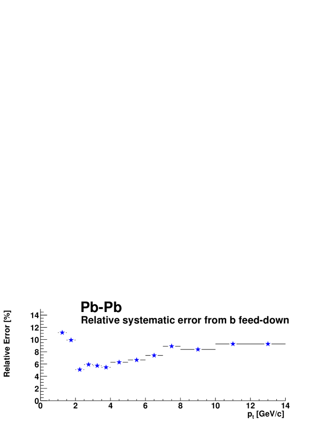
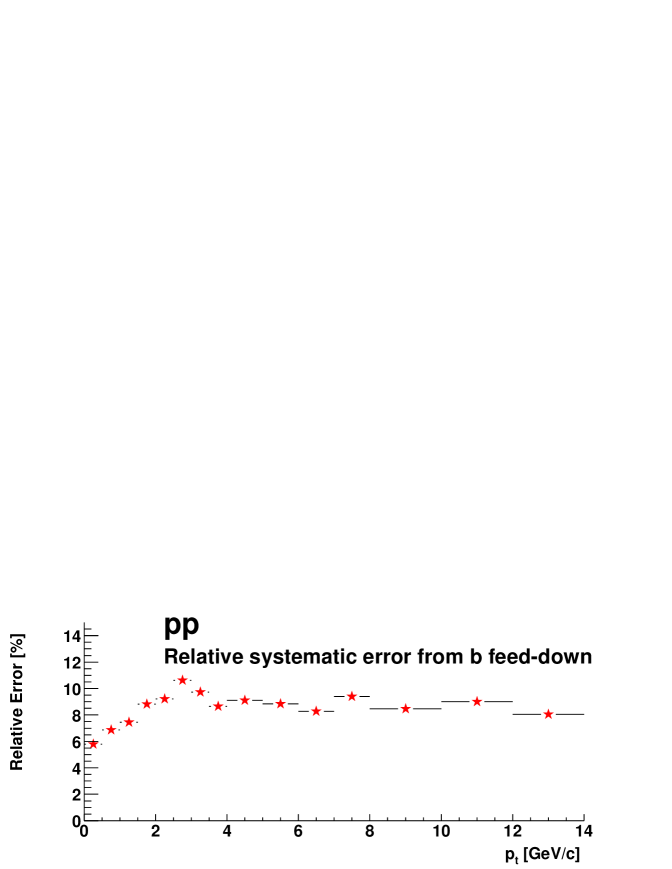
Figure 7.7: Relative systematic error from the correction for feed-down from beauty, in Pb–Pb (top) and pp (bottom).

7.2.2 Cross section normalization

In proton–proton collisions, the cross section for $\mathrm{D^{0}}$ production, which is necessary for example for the comparison with pQCD calculations, can be determined multiplying the estimated number of (primary) $\mathrm{D^{0}}$ produced per inelastic event by the inelastic pp cross section at $\sqrt{s}=14\leavevmode\nobreak\ \mathrm{TeV}$:

$$\sigma_{\rm pp}(\mbox{$\mathrm{D^{0}}$})=N_{\rm pp}(\mbox{$\mathrm{D^{0}}$})/{\rm inel.\leavevmode\nobreak\ event}\times\sigma^{\rm inel}_{\rm pp}.$$ (7.3)

The pp cross section will be measured at the LHC by the TOTEM experiment [97] with an expected precision of about 5%. Therefore, the normalization of $\mathrm{D^{0}}$ production to pp inelastic collisions will contribute a systematic error of $\simeq 5\%$, of course independent of $p_{\rm t}$.

In the case of central nucleus–nucleus collisions, the $\mathrm{D^{0}}$ production cross section per binary NN collision, which enters in the calculation of the nuclear modification factor (Section 2.5.2), can be derived as:

$$\sigma_{\scriptscriptstyle{\rm NN}}(\mbox{$\mathrm{D^{0}}$})=N_{\rm AA}(\mbox{$\mathrm{D^{0}}$})/{\rm event}/R(b_{c}),$$ (7.4)

where $R(b_{c})$, defined in Eq. (3.13), is essentially the average number of binary NN collisions in an AA collision with impact parameter $b<b_{c}$, divided by the inelastic AA cross section corresponding to the same impact parameter range. Three sources contribute to the error on $R(b_{c})$:

1. Error on the centrality selection, i.e. on the determination of the upper limit $b_{c}$ ($\simeq 3.5\leavevmode\nobreak\ \mathrm{fm}$) in impact parameter for the class of most central Pb–Pb collisions (5% of the total cross section). The impact parameter, as mentioned in Chapter 4, is measured in ALICE by means of the Zero Degree Calorimeters, which are expected to provide a relative precision $\delta b/b\simeq 30\%$ for $b<3$-$4\leavevmode\nobreak\ \mathrm{fm}$ [98]. The upper limit will be, therefore, determined as $b_{c}=(3.5\pm 1.0)\leavevmode\nobreak\ \mathrm{fm}$, which gives $R(b_{c})=(27\pm 2)\leavevmode\nobreak\ \mathrm{mb}^{-1}$ (from Fig. 3.4, right panel). The relative error on $R(b_{c})$ and on $\sigma_{\scriptscriptstyle{\rm NN}}(\mbox{$\mathrm{D^{0}}$})$ from this source is then $2/27\simeq 8\%$.

2. Error on the NN inelastic cross section at $\sqrt{s}=5.5\leavevmode\nobreak\ \mathrm{TeV}$. Once the cross section will be measured at $\sqrt{s}=14\leavevmode\nobreak\ \mathrm{TeV}$ by TOTEM, the extrapolation to lower energy should not introduce large additional uncertainties. We, therefore, assume a 5% precision also at 5.5 TeV.

3. Uncertainty on the parameters of the Wood-Saxon nuclear density profile. These uncertainties are of order 5% [68].

Combining these three contributions we obtain an overall normalization error of about 11% for central Pb–Pb collisions.

7.3 Errors on ${\rm d}^{2}\sigma(\mbox{$\mathrm{D^{0}}$})/{\rm d}p_{\rm t}{\rm d}y$ and ${\rm d}\sigma(\mbox{$\mathrm{D^{0}}$})/{\rm d}y$

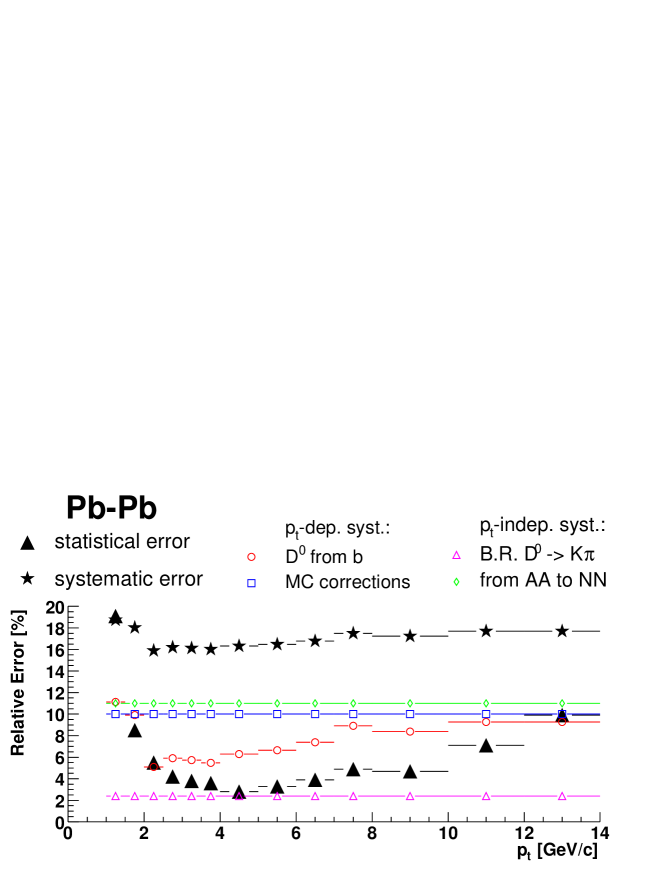
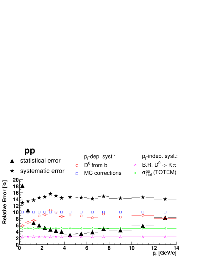
Figure 7.8: Summary of relative errors in Pb–Pb and pp collisions.

The relative statistical errors and the different contributions to the relative systematic errors are summarized in Fig. 7.8. The total systematic error, obtained as a quadratic sum of the single contributions, amounts to 16-17% for the Pb–Pb case and 14-15% for the pp case. However, we remark that (a) some of the systematic errors do not affect the shape of the $p_{\rm t}$ distributions (uncertainty on branching ratio and normalization errors) and (b) many of them are common to Pb–Pb and pp and will cancel in the ratio $R_{\rm AA}$ (correction for b feed-down, branching ratio, uncertainty on NN cross section and, partially, Monte Carlo corrections, e.g. acceptance).

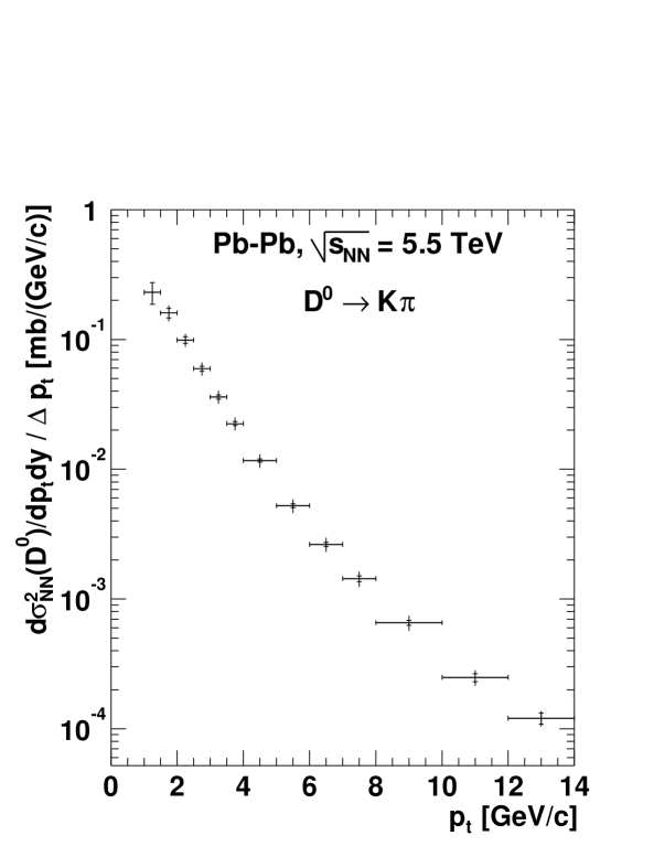
Figure 7.9: Double differential cross section per nucleon–nucleon collision for $\mathrm{D^{0}}$ production as a function of $p_{\rm t}$, as it can be measured with $10^{7}$ central Pb–Pb events. Statistical (inner bars) and $p_{\rm t}$-dependent systematic errors (outer bars) are shown. A normalization error of 11% is not shown.

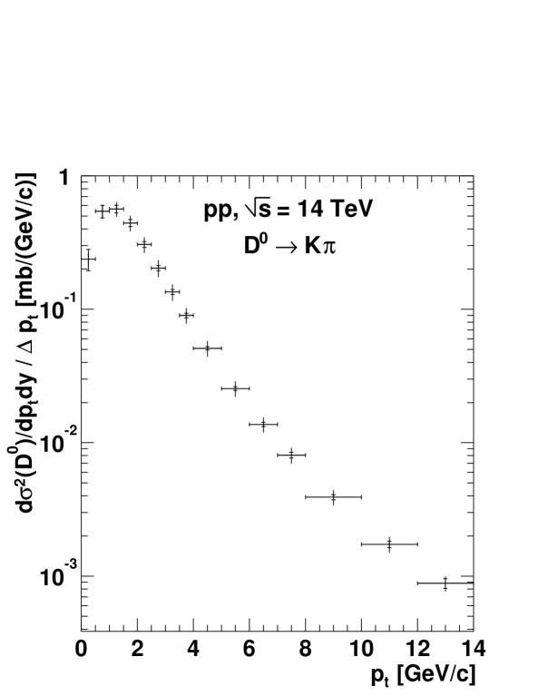
Figure 7.10: Double differential cross section for $\mathrm{D^{0}}$ production as a function of $p_{\rm t}$, as it can be measured with $10^{9}$ pp events. Statistical (inner bars) and $p_{\rm t}$-dependent systematic errors (outer bars) are shown. A normalization error of 5% is not shown.

Figures 7.9 and 7.10 present the distributions of d${}^{2}\sigma(\mbox{$\mathrm{D^{0}}$})/$d$p_{\rm t}$d$y$ in $|y|<1$ with the estimated statistical (inner) and $p_{\rm t}$-dependent systematic (outer) error bars. A normalization error of 11% for Pb–Pb and 5% for pp is not included in the error bars, as it will not affect the shape of the transverse momentum distribution.

The expected relative uncertainties for the measurement of the $\mathrm{D^{0}}$ production cross section per unit of rapidity, integrated over $p_{\rm t}>p_{\rm t}^{\rm min}=1\leavevmode\nobreak\ \mathrm{GeV}/c$ for Pb–Pb and $p_{\rm t}>p_{\rm t}^{\rm min}=0.5\leavevmode\nobreak\ \mathrm{GeV}/c$ for pp, are reported in Table 7.2. The statistical uncertainty was obtained as a quadratic sum of the statistical errors of the $p_{\rm t}$-bins for $p_{\rm t}>p_{\rm t}^{\rm min}$. The single contributions to the systematic uncertainty were obtained as a linear sum over the $p_{\rm t}$-bins and they were then added in quadrature to get the total systematic uncertainty.

Concerning the pp result, we remark that, with statistical and systematic errors of 3% and 14%, and $p_{\rm t}^{\rm min}=0.5\leavevmode\nobreak\ \mathrm{GeV}/c$, the reconstruction of ${\rm D^{0}\to K^{-}\pi^{+}}$ decays in ALICE will provide the only precise measurement of charm production cross section at LHC energy. For comparison, the CDF Collaboration has recently measured $\mathrm{D^{0}}$ production in ${\rm p\overline{p}}$ collisions at the Tevatron, $\sqrt{s}=1.96\leavevmode\nobreak\ \mathrm{TeV}$, with similar uncertainties, 1.5% statistical and 11% systematic, but with a much higher low-$p_{\rm t}$ cut-off, $p_{\rm t}^{\rm min}=5.5\leavevmode\nobreak\ \mathrm{GeV}/c$ [96].

Table 7.2: Expected relative uncertainties for the measurement of d$\sigma(\mbox{$\mathrm{D^{0}}$})/$d$y$ in $|y|<1$ and $p_{\rm t}>p_{\rm t}^{\rm min}$.

System	Pb–Pb	pp
	$p_{\rm t}^{\rm min}=1\leavevmode\nobreak\ \mathrm{GeV}/c$	$p_{\rm t}^{\rm min}=0.5\leavevmode\nobreak\ \mathrm{GeV}/c$
Statistical error	7%	3%
Systematic error	17%	14%
Correction for b feed-down	9%	8%
Monte Carlo corrections	10%	10%
Branching ratio	2%	2%
Cross section normalization	11%	5%

7.4 Comparison with pQCD predictions

In Section 3.1 we have seen that the results of perturbative QCD calculations for $\mathrm{c\overline{c}}$ (and $\mathrm{b\overline{b}}$) production at the LHC have a strong dependence on the choice of the heavy quark masses and of the factorization and renormalization scales, $\mu_{F}$ and $\mu_{R}$. We compare here to this theoretical uncertainty the sensitivity of ALICE for the measurement of the total and $p_{\rm t}$-differential cross section for $\mathrm{D^{0}}$ production in pp collisions at $14\leavevmode\nobreak\ \mathrm{TeV}$. We used the program by Mangano, Nason and Ridolfi (HVQMNR) [64] to calculate the cross sections for different sets of parameters. The $p_{\rm t}$ distributions for D mesons were obtained from those for c quarks using the PYTHIA fragmentation model (more details on the procedure are given in the next chapter, Section 8.2).

Figure 7.11 shows the comparison for d$\sigma(\mbox{$\mathrm{D^{0}}$})/$d$y$, integrated for $p_{\rm t}>0.5\leavevmode\nobreak\ \mathrm{GeV}/c$. Statistical (narrower) and systematic (broader) error bands are reported; the latter include all normalization errors. The error bars are hereafter applied to the value obtained with the set of parameters used in our simulations (‘default parameters’): $m_{\rm c}=1.2\leavevmode\nobreak\ \mathrm{GeV}$, $\mu_{F}=\mu_{R}=2\mu_{0}=2\sqrt{(p_{\rm t,c}^{2}+p_{\rm t,\overline{c}}^{2})/2+m_{\rm c}^{2}}$ and PDF set = CTEQ 4M. The comparison for the $p_{\rm t}$-differential cross section is presented in Fig. 7.12 along with the ratio ‘theory/data’ (‘theory parameters/default parameters’) which better allows to compare the different $p_{\rm t}$-shapes obtained by changing the input ‘theory parameters’ and to illustrate the sensitivity of the ALICE measurement.

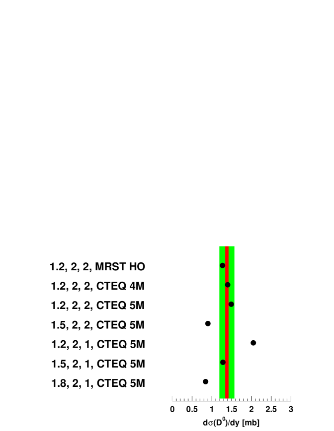
Figure 7.11: ALICE sensitivity on d$\sigma(\mbox{$\mathrm{D^{0}}$})/$d$y$ integrated for $p_{\rm t}>0.5\leavevmode\nobreak\ \mathrm{GeV}/c$, in pp at 14 TeV, compared to the pQCD predictions obtained with different sets of the input parameters $m_{\rm c}$ [GeV], $\mu_{F}/\mu_{0}$, $\mu_{R}/\mu_{0}$ and PDF set ($\mu_{0}$ is defined in the text). The narrower band represents the statistical error, the broader band the systematic error, including all normalization errors.

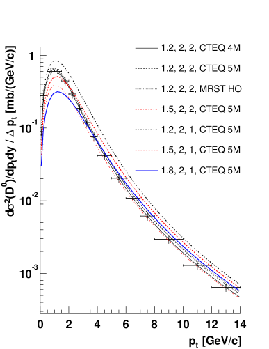
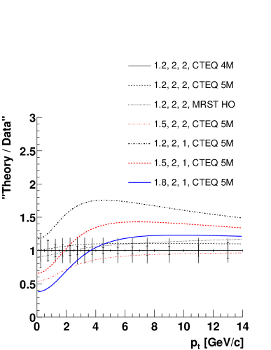
Figure 7.12: ALICE sensitivity on d${}^{2}\sigma(\mbox{$\mathrm{D^{0}}$})/$d$p_{\rm t}$d$y$, in pp at 14 TeV, compared to the pQCD predictions obtained with different sets of the input parameters $m_{\rm c}$ [GeV], $\mu_{F}/\mu_{0}$, $\mu_{R}/\mu_{0}$ and PDF set ($\mu_{0}$ is defined in the text). The inner bars represent the statistical error, the outer bars the $p_{\rm t}$-dependent systematic error. A normalization error of 5% is not shown. The panel on the right shows how a ‘theory/data’ plot could look like.

7.5 Energy extrapolation of the pp result

The comparison plots presented in the previous section show that the measurement of $\mathrm{D^{0}}$ production in pp collisions at 14 TeV will be accurate enough to allow some kind of ‘tuning’ of the pQCD calculations by choosing the set/sets of input parameters that better reproduce the experimental total cross section and $p_{\rm t}$ distribution.

After such parameter selection, perturbative QCD can be used for the extrapolation of pp results from 14 to 5.5 TeV. We remind that this step is necessary in order to calculate the nuclear modification factor $R_{\rm AA}$.

In Chapter 3 (Table 3.2) we showed that the ratio of the total $\mathrm{c\overline{c}}$ cross section at different energies is almost independent of the input parameters used. We consider here this point more in detail by comparing the ratios of the $p_{\rm t}$-differential $\mathrm{D^{0}}$ cross sections at 14 and at 5.5 TeV for different sets of parameters. The result is reported in Fig. 7.13: the ratio is independent of the input parameters within 10% up to $p_{\rm t}=20\leavevmode\nobreak\ \mathrm{GeV}/c$. Therefore, the ‘tuning’ of the parameters has only a marginal importance, since the $p_{\rm t}$ distribution measured at 14 TeV allows to predict the $p_{\rm t}$ distribution at 5.5 TeV. The spread in the ratio displayed in Fig. 7.13 can be taken as an estimate of the error introduced by the energy extrapolation; such error shall be accounted for in the evaluation of the sensitivity on $R_{\rm AA}$ in Chapter 8.

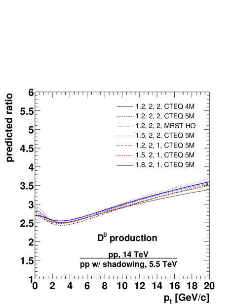
Figure 7.13: Ratio of the $p_{\rm t}$-differential $\mathrm{D^{0}}$ cross section given by pQCD at 14 and at 5.5 TeV for different sets of the input parameters: $m_{\rm c}$ [GeV], $\mu_{F}/\mu_{0}$, $\mu_{R}/\mu_{0}$ and PDF set.

7.6 Perspectives for the measurement of
$N({\rm b\to B\to D^{0}})/N({\rm c\to D^{0}})$

Primary and secondary $\mathrm{D^{0}}$ mesons can, in principle, be separated on the basis of their impact parameter to the interaction vertex. For a $\mathrm{D^{0}}$ with reconstructed decay vertex $(V_{x},V_{y},V_{z})$ and reconstructed momentum at the decay vertex $(p_{x},p_{y},p_{z})$, the impact parameter in the transverse plane is defined as the distance of the straight line parameterized as $(V_{x},V_{y})+k\,(p_{x},p_{y})$ to the reconstructed position of the interaction vertex in the transverse plane. For $\mathrm{D^{0}}$ mesons coming from c quarks, the impact parameter should be 0, within the experimental resolution, while for $\mathrm{D^{0}}$ mesons coming from the decay of B mesons, it should differ significantly from 0, as B mesons have a mean decay length of order $500\leavevmode\nobreak\ \mathrm{\mu m}$. However, the separation may not be very clear because, in the B decay, the $\mathrm{D^{0}}$ is the heavier particle and it tends to carry most of the momentum of the B and, consequently, to follow its flight direction, thus having a small impact parameter.

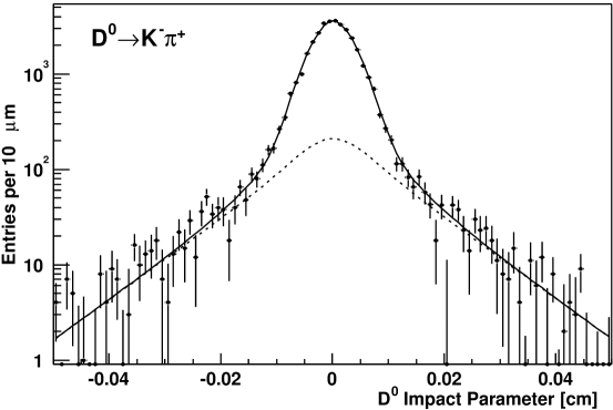
Figure 7.14: CDF data: the impact parameter distribution of $\mathrm{D^{0}}$ mesons, measured from the $\pm 2\leavevmode\nobreak\ \sigma$ signal region of the invariant mass distribution and corrected for combinatorial background measured in the invariant mass side-bands. The dashed curve shows the contribution of secondary $\mathrm{D^{0}}$ from B decays [96].

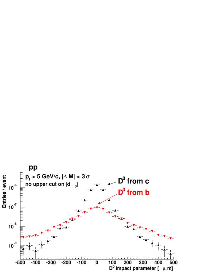
Figure 7.15: Impact parameter distribution for primary and secondary $\mathrm{D^{0}}$ mesons in pp collisions. All detector and reconstruction effects are taken into account, including the reconstruction of the interaction vertex position using tracks.

As mentioned, the analysis of the $\mathrm{D^{0}}$ impact parameter has been done by the CDF Collaboration on the data collected in Run II at the Tevatron. Figure 7.14 shows the distribution of this variable for signal $\mathrm{D^{0}}$ candidates with invariant mass in the range $M_{\rm D^{0}}\pm 2\leavevmode\nobreak\ \sigma$ and with $p_{\rm t}>5.5\leavevmode\nobreak\ \mathrm{GeV}/c$ [96]. The contribution of the combinatorial background has been subtracted. This can be done because the integral of the background is known from the fit of the invariant mass distribution and its shape is obtained from the impact parameter distribution of the $\mathrm{D^{0}}$ candidates that populate the side-bands of the invariant mass ($|M-M_{\rm D^{0}}|>4\leavevmode\nobreak\ \sigma$). The true impact parameter of primary $\mathrm{D^{0}}$ is 0, while the shape of the true impact parameter distribution of secondary $\mathrm{D^{0}}$ is derived from a generator-level Monte Carlo simulation of B meson production and decay. Both components are smeared with a resolution function (Gaussian + exponential tails) obtained from a sample of ${\rm K^{0}_{S}}\to\pi^{+}\pi^{-}$ (${\rm K^{0}_{S}}$ are almost exclusively primary, thus having true impact parameter equal to 0). In this way the shapes of the two distributions for primary and secondary $\mathrm{D^{0}}$ are known and their relative integral is obtained from a fit. Averaged over $p_{\rm t}>5.5\leavevmode\nobreak\ \mathrm{GeV}/c$, the fraction of primary $\mathrm{D^{0}}$ is estimated to be $(86.6\pm 0.4({\rm stat})\pm 3.0({\rm syst}))\%$ [96].

We reported a detailed description of the analysis performed in CDF, because the idea is to apply the same strategy in ALICE, not only in pp but also in Pb–Pb events. A preliminary study was carried out and the results, shown in the following, are quite promising.

The impact parameter distribution for selected $\mathrm{D^{0}}$ candidates in pp events is presented in Fig. 7.15. The contributions of signal $\mathrm{D^{0}}$ from c and from b are plotted separately. The cuts reported in Table 6.9 are applied; only the cut on the maximum value of the impact parameter of the decay tracks, which would suppress the component of $\mathrm{D^{0}}$ from b, is removed. The additional cuts $|M-M_{\rm D^{0}}|<3\leavevmode\nobreak\ \sigma$ and $p_{\rm t}>5\leavevmode\nobreak\ \mathrm{GeV}/c$ are applied. All detector and reconstruction effects are taken into account, including the reconstruction of the interaction vertex position using tracks. The distributions of primary and secondary $\mathrm{D^{0}}$ have significantly different shapes, similarly to what observed by CDF.

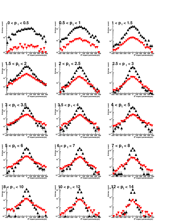
Figure 7.16: Impact parameter distribution for primary (triangle up) and secondary (triangle down) $\mathrm{D^{0}}$ mesons in pp collisions, in bins of the $\mathrm{D^{0}}$ transverse momentum.

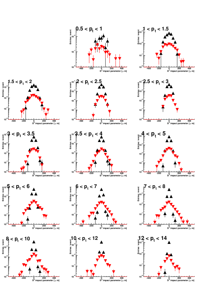
Figure 7.17: Impact parameter distribution for primary (triangle up) and secondary (triangle down) $\mathrm{D^{0}}$ mesons in Pb–Pb collisions, in bins of the $\mathrm{D^{0}}$ transverse momentum.

The same distributions are shown in bins of $p_{\rm t}$ in Figs. 7.16 and 7.17 for pp and Pb–Pb, respectively. In both cases, the difference in shape between the two contributions is visible down to $p_{\rm t}\simeq 4$-$5\leavevmode\nobreak\ \mathrm{GeV}/c$; for lower $p_{\rm t}$ the resolution on the position of the $\mathrm{D^{0}}$ decay vertex is quite poor due to multiple scattering effects and the impact parameter distribution of primary $\mathrm{D^{0}}$ mesons becomes very broad. We point out that the separation is sharper in Pb–Pb than in pp collisions, since the resolution on the transverse position of the interaction vertex is better (see Chapter 5).

More detailed investigations are necessary for a clear assessment of the feasibility of an analysis ‘à la CDF’. In particular, the effect of the cut on the pointing angle should be evaluated and the strategy for background subtraction and fit of the two signal components should be studied. However, there are good indications of the possibility to measure the ratio of primary to secondary $\mathrm{D^{0}}$ mesons as a function of $p_{\rm t}$, down to $4$-$5\leavevmode\nobreak\ \mathrm{GeV}/c$, in pp, p–Pb and Pb–Pb collisions. This would allow a direct correction of the $\mathrm{D^{0}}$ yield for feed-down from B decays and might provide information on the ratio of B/D mesons as a function of $p_{\rm t}$, which is regarded as particularly interesting to investigate the mass dependence of medium-induced energy loss for heavy quarks (see Section 2.3.3).

Chapter 8 Quenching of open charm mesons

The role of a comparative analysis of the quenching of charm mesons and charged hadrons in the scope of a systematic study of the properties of QCD matter produced in Pb–Pb collisions at the LHC was emphasized in Chapter 2. In this chapter we evaluate the effect of medium-induced energy loss on the transverse momentum distributions of c quarks and D mesons and we discuss the potential of ALICE for carrying out such comparative analysis.

The choice of the input parameters for the simulation of energy loss is considered in Section 8.1. We derive the distribution of in-medium path lengths using a detailed description of the collision geometry and we estimate a value for the transport coefficient of the medium at the LHC, keeping into account the pion suppression observed in Au–Au collisions at RHIC (see Section 1.3). In Section 8.2 we describe how the SW (Salgado-Wiedemann) weights (Section 2.3.2) are used to quench charm quarks and D mesons generated with PYTHIA and we introduce a correction to the weights that accounts for the dead cone effect predicted for heavy quarks. The nuclear modification factor of D mesons and the D/$hadrons$ ratio for different quenching scenarios (different transport coefficients, dead cone option) are presented in Sections 8.3 and 8.4. The attainable precision in the measurement of these observables is derived from the uncertainties on the $p_{\rm t}$ distributions estimated in Chapter 7.

8.1 Medium parameters: path length and transport coefficient

The distribution of the in-medium path length in the transverse plane, $L$, for central Pb–Pb collisions (impact parameter $b<3.5\leavevmode\nobreak\ \mathrm{fm}$) is calculated in the framework of the Glauber model of the collision geometry. We refer to the nomenclature introduced in Section 3.2.1. For fixed impact parameter, the density of binary NN collisions in the transverse plane is obtained as the product of the thickness functions of the two colliding Pb nuclei, $T_{\rm A}(\vec{s})\,T_{\rm B}(\vec{s}-\vec{b})$; parton production points are sampled according to this density and their azimuthal propagation directions are sampled uniformly in the range $[0,2\pi]$. For a parton with given production point $(x_{0},y_{0})$ and azimuthal direction $\phi_{0}$ (see Fig. 8.2), the path length $L$ is defined as the line integral from the production point to ‘well outside the superposition region of the two nuclei’ weighted by the product of the thickness functions and normalized with its integral:

$$L=\frac{\int_{0}^{\infty}{\rm d}l\,l\,T_{\rm A}(\vec{s}(l))\,T_{\rm B}(\vec{s}(l)-\vec{b})}{0.5\,\int_{0}^{\infty}{\rm d}l\,T_{\rm A}(\vec{s}(l))\,T_{\rm B}(\vec{s}(l)-\vec{b})}.$$ (8.1)

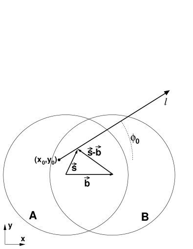
Figure 8.1: Geometry of the collision in the transverse plane and definition of the in-medium path length.

Figure 8.2: Distribution of the path lengths in the transverse plane for partons produced in Pb–Pb collisions with $b<3.5\leavevmode\nobreak\ \mathrm{fm}$ (5% of the inelastic cross section).

Many sampling iterations are performed varying the impact parameter $b$ from $0.25\leavevmode\nobreak\ \mathrm{fm}$ to $3.25\leavevmode\nobreak\ \mathrm{fm}$ in steps of $0.5\leavevmode\nobreak\ \mathrm{fm}$. The obtained distributions are given a weight $b$, since we verified that d$\sigma^{\rm hard}/$d$b\propto b$ for $b<3.5\leavevmode\nobreak\ \mathrm{fm}$, and added together. The result is shown in Fig. 8.2. The average length is $4.5\leavevmode\nobreak\ \mathrm{fm}$, corresponding to about 70% of the radius of a Pb nucleus and the distribution is significantly accumulated towards low values of $L$ because a large fraction of the partons are produced in the periphery of the superposition region of the two nuclei (‘corona’ effect).  

For the estimation of the value of the other input parameter, the transport coefficient $\hat{q}$, we consider that it is reasonable to require for AA collisions at the LHC a quenching of hard partons of the same magnitude as that observed at RHIC. We, therefore, derive the nuclear modification factor $R_{\rm AA}$ for charged hadrons produced at the LHC and we choose the transport coefficient in order to obtain $R_{\rm AA}\simeq 0.2$-$0.3$ in the range $p_{\rm t}=5$-$10\leavevmode\nobreak\ \mathrm{GeV}/c$ (PHENIX results were reported in Fig. 1.7).

The transverse momentum distributions, for $p_{\rm t}>5\leavevmode\nobreak\ \mathrm{GeV}/c$, of charged hadrons are generated by means of the chain:

1. generation of a parton, quark or gluon, with $p_{\rm t}>5\leavevmode\nobreak\ \mathrm{GeV}/c$;

2. sampling of an energy loss $\Delta E$ and calculation of the quenched transverse momentum of the parton, $p_{\rm t}^{\prime}=p_{\rm t}-\Delta E$ (if $\Delta E>p_{\rm t}$, $p_{\rm t}^{\prime}$ is set to 0);

3. (independent) fragmentation of the parton to a hadron.

Quenched and unquenched $p_{\rm t}$ distributions are obtained including or excluding the second step of the chain. We shall now detail each single step.

Input $p_{\rm t}$ distributions of quarks and gluons are generated in PYTHIA with the same settings used for the generation of pp events at $\sqrt{s}=14\leavevmode\nobreak\ \mathrm{TeV}$ (Section 4.2.1), except the c.m.s. energy, which was set to $5.5\leavevmode\nobreak\ \mathrm{TeV}$. The CTEQ 4L set of parton distribution functions was used. Figure 8.3 (left) reports the result of a fit on the $p_{\rm t}$ distributions of quarks and gluons for $p_{\rm t}>5\leavevmode\nobreak\ \mathrm{GeV}/c$. With this $p_{\rm t}$ cut, the parton composition is found to be 78% gluons and 22% quarks, with the ratio quarks/gluons increasing with $p_{\rm t}$ (i.e. with Bjorken $x$), as the contribution of the valence quarks of the incoming protons becomes more and more important (see parton distributions in Fig. 1.12).

For the fragmentation (step 3) we use the leading order (LO) Kniehl-Kramer-Pötter (KKP) fragmentation functions [99]. This kind of fragmentation procedure is called independent, as each parton fragments to a single hadron with transverse momentum $p_{\rm t}^{\rm hadron}=z\,E^{\rm parton}\simeq z\,p_{\rm t}^{\rm parton}$ (see Fig. 8.3, right). We choose such approach, rather than using the standard string fragmentation of PYTHIA, because this would require the implementation of partonic energy loss in PYTHIA, which is highly non-trivial and goes beyond the scope of this work. In the next section we will show that a simple Charm quantum number conservation argument allows to use the PYTHIA string fragmentation in the calculations for the quenching of D mesons.

The quenching procedure is as follows. As described in Section 2.3.2, the SW quenching weight has a discrete part $p_{0}$ ($\equiv$ probability to have no gluon radiation) and a continuous part $p(\Delta E)$ ($\equiv$ probability to radiate an energy $\Delta E$, if at least one gluon is radiated). Both parts of the weight have to be included in the quenching procedure. In addition, the Glauber-based distribution of path lengths $L$ has to be accounted for.

For a given value of the transport coefficient $\hat{q}$ and a given parton species (quark or gluon), we use the routine provided by the authors [51] to get $p_{0}$ and to histogram the distribution $p(\Delta E)$ for all integer values of $L$ up to $15\leavevmode\nobreak\ \mathrm{fm}$ ($1\leavevmode\nobreak\ \mathrm{fm}$, $2\leavevmode\nobreak\ \mathrm{fm}$, …, $15\leavevmode\nobreak\ \mathrm{fm}$). Since $p_{0}$ is essentially a probability to have $\Delta E=0$ (no radiated gluons), we add the value of $p_{0}$ to the bin corresponding to $\Delta E=0$ in the histogram of the continuous part of the weight $p(\Delta E)$. In this way the complete distribution of energy loss probability, including both parts of the quenching weight and properly normalized, is obtained for each value of $L$. Finally, these 15 distributions are weighted according to the path length distribution in Fig. 8.2 and added together. The resulting energy loss probability distributions $P(\Delta E)$ for quarks in media with $\hat{q}=0.05\leavevmode\nobreak\ \mathrm{GeV}^{2}/\mathrm{fm}$ (cold medium) and $\hat{q}=1\leavevmode\nobreak\ \mathrm{GeV}^{2}/\mathrm{fm}$ (hot medium) are reported in Fig. 8.4 (the ‘peak’ at $\Delta E=0$ represents the discrete part of the quenching weight). The energy loss to be used in the second step of the chain reported above can be directly sampled from the $P(\Delta E)$ distribution corresponding to the chosen $\hat{q}$ and to the correct parton species.

Figure 8.3: Left: fitted transverse momentum distributions for quarks and gluons generated with PYTHIA; the sum of quarks and gluons is shown as well. Right: KKP fragmentation functions for quarks and gluons into hadrons, with a cut $p_{\rm t}^{\rm hadron}>5\leavevmode\nobreak\ \mathrm{GeV}/c$.

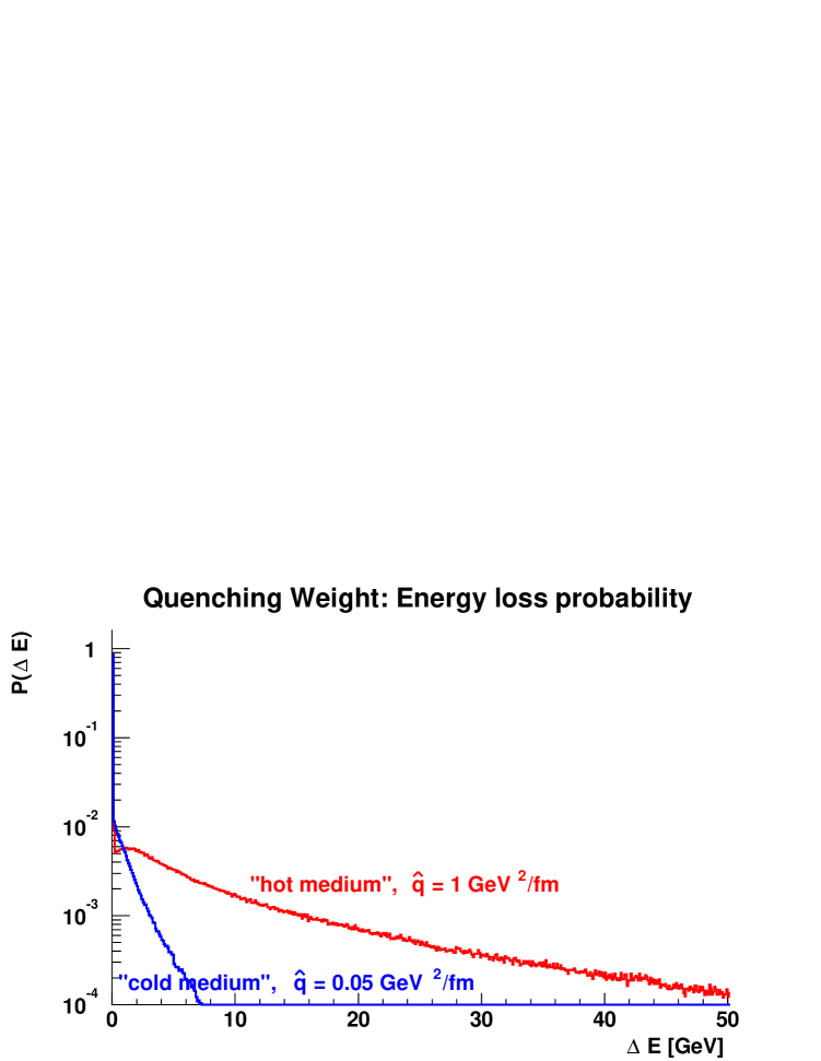
Figure 8.4: Quark energy loss probability for $\hat{q}=0.05\leavevmode\nobreak\ \mathrm{GeV}^{2}/\mathrm{fm}$ and for $\hat{q}=1\leavevmode\nobreak\ \mathrm{GeV}^{2}/\mathrm{fm}$. The discrete and the continuous parts of the quenching weight are included and the distribution of in-medium path lengths is taken into account.

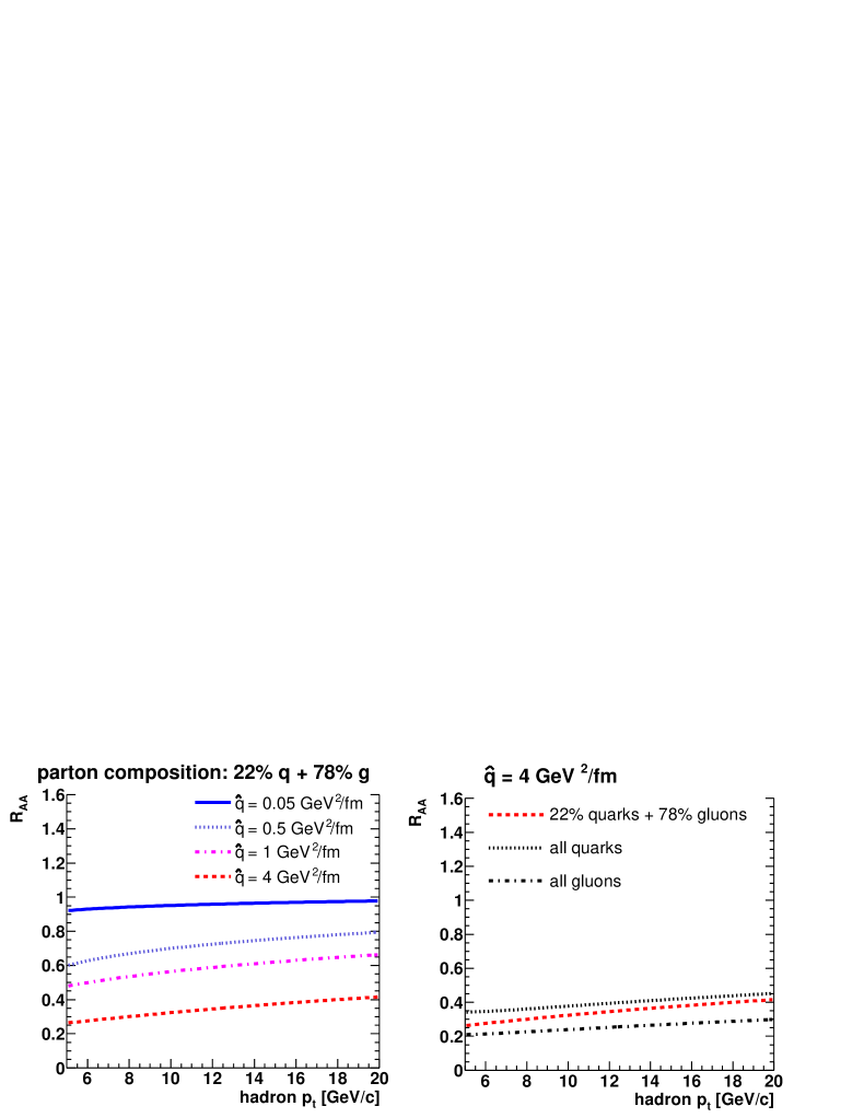
Figure 8.5: Left: nuclear modification factor for charged hadrons for different values of $\hat{q}$. Right: comparison of quark and gluon quenching for $\hat{q}=4\leavevmode\nobreak\ \mathrm{GeV}^{2}/\mathrm{fm}$.

Experimentally, the nuclear modification factor will be obtained as the ratio of the $p_{\rm t}$ distribution measured in central Pb–Pb collisions at $\sqrt{s_{\scriptscriptstyle{{\rm NN}}}}=5.5\leavevmode\nobreak\ \mathrm{TeV}$, divided by the estimated number of binary collisions, to the $p_{\rm t}$ distribution measured in pp collisions at $\sqrt{s}=14\leavevmode\nobreak\ \mathrm{TeV}$, extrapolated to $\sqrt{s}=5.5\leavevmode\nobreak\ \mathrm{TeV}$ by means of pQCD. Here, for the moment, we go directly to $R_{\rm AA}$ (the uncertainties involved in the experimental estimate will be discussed in the last part of this chapter). Figure 8.5 shows $R_{\rm AA}$ for hadrons, calculated as the ratio of the $p_{\rm t}$ distribution with quenching to the $p_{\rm t}$ distribution without quenching. Different values of $\hat{q}$ are considered in the left panel of the figure: a value as large as $4\leavevmode\nobreak\ \mathrm{GeV}^{2}/\mathrm{fm}$ is necessary to have $R_{\rm AA}\simeq 0.25$-$0.3$ in $5<p_{\rm t}<10\leavevmode\nobreak\ \mathrm{GeV}/c$. In the right panel, for $\hat{q}=4\leavevmode\nobreak\ \mathrm{GeV}^{2}/\mathrm{fm}$, we compare the results obtained considering all partons as gluons or all partons as quarks, in order to remark and quantify the larger quenching of gluons with respect to quarks.

Since the transport coefficient determines the size of the energy loss effect, we shortly discuss the choice of $\hat{q}=4\leavevmode\nobreak\ \mathrm{GeV}^{2}/\mathrm{fm}$. This value corresponds, using the plot in Fig. 2.3, to an energy density $\varepsilon\simeq 40$-$50\leavevmode\nobreak\ \mathrm{GeV}/\mathrm{fm}^{3}$, which is about a factor 2 lower than the maximum energy density expected for central Pb–Pb collisions at the LHC (see Table 1.1). The value looks, therefore, reasonable.

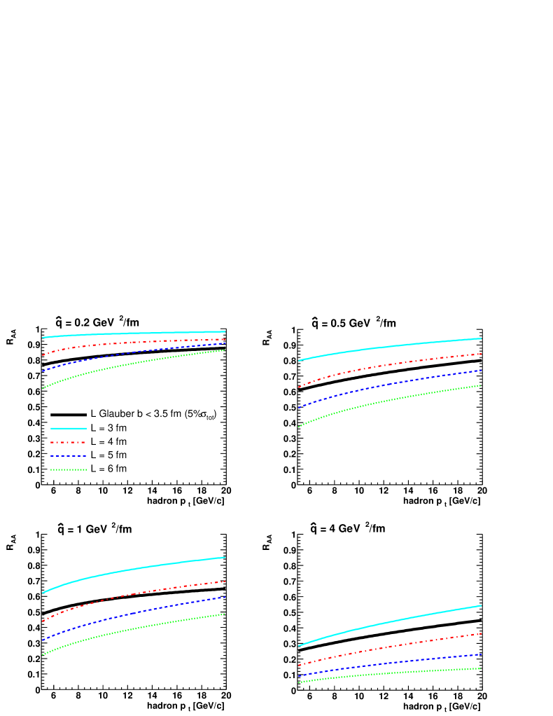
Figure 8.6: Nuclear modification factor for charged hadrons for different values of $\hat{q}$ as obtained using the complete Glauber-based distribution or constant values of $L$.

Using the same quenching weights, Salgado and Wiedemann reproduce the suppression observed at RHIC with the much lower value $\hat{q}=0.75\leavevmode\nobreak\ \mathrm{GeV}^{2}/\mathrm{fm}$ [51]. However, they use the constant length $L=6\leavevmode\nobreak\ \mathrm{fm}$ rather than a realistic distribution of lengths, thus obtaining a significantly stronger quenching.

The use of a constant length of the order of the nuclear radius or even the use of the average length from a detailed distribution can produce quite different results with respect to those obtained keeping into account the complete distribution. This is demonstrated in Fig. 8.6: for $\hat{q}=0.5$-$1\leavevmode\nobreak\ \mathrm{GeV}^{2}/\mathrm{fm}$, $L=6\leavevmode\nobreak\ \mathrm{fm}$ gives almost a factor 2 difference in $R_{\rm AA}$ at $p_{\rm t}\sim 10\leavevmode\nobreak\ \mathrm{GeV}/c$ and the complete $L$ distribution is equivalent to a constant length which decreases as $\hat{q}$ increases, 5, 4.5, 4, 3.5 fm for $\hat{q}=0.2,\leavevmode\nobreak\ 0.5,\leavevmode\nobreak\ 1,\leavevmode\nobreak\ 4\leavevmode\nobreak\ \mathrm{GeV}^{2}/\mathrm{fm}$. This behaviour is clearly due to an upper ‘cut-off’ of the length distribution: large lengths correspond to very high values of $\Delta E$, but, since $\Delta E$ cannot be higher than the initial parton energy, large lengths are not ‘fully exploited’; this corresponds to a cut-off; e.g. for many partons of moderate energy a length of $8\leavevmode\nobreak\ \mathrm{fm}$ is equivalent to a length of $4\leavevmode\nobreak\ \mathrm{fm}$, because after propagating for $4\leavevmode\nobreak\ \mathrm{fm}$ they have lost all their initial energy. As a consequence, the length distribution corresponds to an average effective length lower than its arithmetic average. The cut-off moves towards lower lengths as $\hat{q}$ increases and, thus, the average effective length decreases. Another important observation revealed by Fig. 8.6 is the fact that the use of the complete $L$ distribution reduces the increase of $R_{\rm AA}$ with $p_{\rm t}$, which is not observed in RHIC data. This happens because higher energy partons can exploit the large-$L$ tail more than lower energy partons and, consequently, for them the cut-off is shifted towards larger lengths.

Finally, we consider that the transport coefficient can be related to the initial gluon rapidity density via the approximated formula [51, 100]:

$$\hat{q}=\frac{2}{R_{\rm A}^{2}\,L}\times\frac{{\rm d}N_{\rm gluons}}{{\rm d}y}$$ (8.2)

where $R_{\rm A}$ is the nuclear radius. For $\hat{q}=4\leavevmode\nobreak\ \mathrm{GeV}^{2}/\mathrm{fm}$, $R_{\rm A}=6\leavevmode\nobreak\ \mathrm{fm}$ and $L=3.5\leavevmode\nobreak\ \mathrm{fm}$ (see bottom-right panel in Fig. 8.6) we obtain d$N_{\rm gluons}/$d$y=6300$. Given the large uncertainties [100] in the relation (8.2), this value is in reasonable agreement with the estimated [26] d$N_{\rm gluons}/$d$y\simeq 5000$ for LHC, reported in Table 1.1.

In summary, we use the in-medium path length distribution shown in Fig. 8.2 for Pb–Pb collisions with $b<3.5\leavevmode\nobreak\ \mathrm{fm}$ and a transport coefficient $\hat{q}=4\leavevmode\nobreak\ \mathrm{GeV}^{2}/\mathrm{fm}$. For comparison, we will as well present the results for lower values of $\hat{q}$.

8.2 Charm energy loss with quenching weights

Energy loss for charm quarks is simulated following a slightly different procedure with respect to that for light quarks and gluons, because (a) the total number of $\mathrm{c\overline{c}}$ pairs per event has to be conserved and (b) the string fragmentation implemented in PYTHIA is more reliable for heavy quarks than the independent fragmentation.

The starting point is the generation with PYTHIA of charm events, each one containing a $\mathrm{c\overline{c}}$ pair. The parameters obtained from the tuning described in Section 3.4 are used for PYTHIA and charm quarks are fragmented to hadrons via the default string model. Since c and $\overline{\rm c}$ quarks fragment to D and $\overline{\rm D}$ mesons, respectively, in each event related ${\rm(c,D)}$ and ${\rm(\overline{c},\overline{D})}$ pairs can be easily identified.

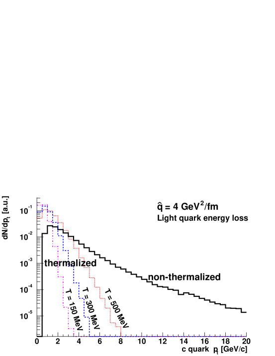
Figure 8.7: $p_{\rm t}$ distributions of non-thermalized ($p_{\rm t}^{\rm c}-\Delta E>1.5\,T$) and thermalized ($p_{\rm t}^{\rm c}-\Delta E<1.5\,T$) c quarks for $\hat{q}=4\leavevmode\nobreak\ \mathrm{GeV}^{2}/\mathrm{fm}$ and $T=150,\,300,\,500\leavevmode\nobreak\ \mathrm{MeV}$ (for clearness the non-thermalized component is shown only for $T=500\leavevmode\nobreak\ \mathrm{MeV}$). The quenching corresponding to light quarks was applied.

The second step consists in applying the quenching to the $p_{\rm t}$ distribution of charm quarks. The procedure is close to that used for light quarks and gluons: for each quark an energy loss $\Delta E$ is sampled from a distribution $P(\Delta E)$ (similar to those shown in Fig. 8.4) and the transverse momentum is modified to $(p_{\rm t}^{\rm c})^{\prime}=p_{\rm t}^{\rm c}-\Delta E$. In Ref. [101] it is pointed out that if the energy loss is close to the transverse momentum of the c quark, or larger than it, the quark should be considered as thermalized with the dense medium. We use $T=300\leavevmode\nobreak\ \mathrm{MeV}$ as the temperature of the medium and, in the cases when $p_{\rm t}^{\rm c}-\Delta E<1.5\,T$, we assign to the quark a thermal transverse momentum according the distribution d$N/$d$m_{\rm t}\propto m_{\rm t}\cdot\exp(-m_{\rm t}/T)$, being $m_{\rm t}=\sqrt{m_{\rm c}^{2}+p_{\rm t}^{2}}$ the transverse mass of the quark. This procedure allows to conserve the number of $\mathrm{c\overline{c}}$ pairs. In Fig. 8.7 we show that the thermalized component accumulates in the region $p_{\rm t}<5$-$6\leavevmode\nobreak\ \mathrm{GeV}/c$ for temperatures up to $T=500\leavevmode\nobreak\ \mathrm{MeV}$, which is a factor 3 larger than the expected thermalization temperature of $170\leavevmode\nobreak\ \mathrm{MeV}$. As mentioned in Chapter 2 and as we shall detail in the next section, the quenching of D mesons can be better studied for $p_{\rm t}>6$-$7\leavevmode\nobreak\ \mathrm{GeV}/c$. We, then, conclude that the choice of $T$ is not critical in our energy loss simulation.

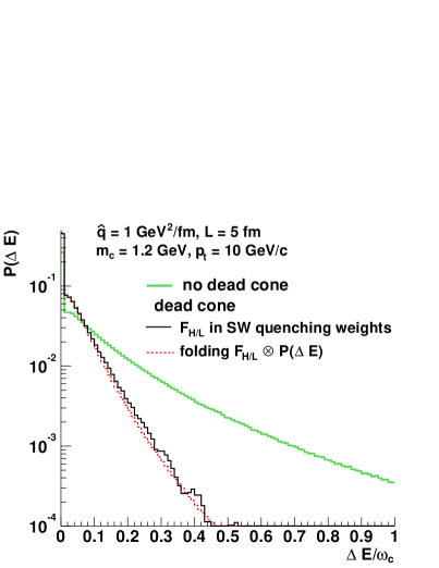
Figure 8.8: Left: multiplicity of medium-induced gluons radiated with energy larger than $\omega$, from Ref. [51]. Right: energy loss probability distribution without dead cone and with the two different implementations of the dead cone effect as described in the text.

As a last step, starting from the unquenched, $N^{\rm vacuum}_{\rm c}(p_{\rm t})$, and quenched, $N^{\rm medium}_{\rm c}(p_{\rm t})$, $p_{\rm t}$ distributions for charm quarks, the quenched $p_{\rm t}$ distribution for D mesons was obtained by applying to each of the mesons generated with PYTHIA the weight:

$$\mathcal{W}(p_{\rm t}^{\rm c})=\frac{N^{\rm medium}_{\rm c}(p_{\rm t}^{\rm c})}{N^{\rm vacuum}_{\rm c}(p_{\rm t}^{\rm c})},$$ (8.3)

where $p_{\rm t}^{\rm c}$ is the original transverse momentum of the parent quark.

The energy loss probability distributions $P(\Delta E)$ for charm quarks were corrected to account for the dead cone effect, described in Section 2.3.3. This was done by folding the distribution $P(\Delta E)$ for light quarks with the dead cone suppression factor introduced in Ref. [53] and reported in Section 2.3.3. In the following we detail and justify this solution.

Figure 8.8 (left) from Ref. [51] shows that for $R\equiv 0.5\,\hat{q}\,L^{3}\simeq 2100$ (with $\hat{q}=4\leavevmode\nobreak\ \mathrm{GeV}^{2}/\mathrm{fm}$ and $L=3.5\leavevmode\nobreak\ \mathrm{fm}$) the average number $N(\omega=0)$ of radiated gluons per parton, when at least 1 gluon is radiated, is approximately 1. If the number of radiated gluons was always 1, the distribution of the continuous part $p(\Delta E)$ of the quenching weight would coincide with the energy distribution d$I/$d$\omega$ of radiated gluons (see Eq. (2.5)). Then, the dead cone suppression factor $F_{\rm H/L}(m_{\rm c},E_{\rm c},\hat{q},\omega)$ in Eq. (2.12), which multiplies d$I/$d$\omega$, could be applied directly to $p(\Delta E)$ with $\omega=\Delta E$. The complete energy loss probability distribution $P(\Delta E)$ is the weighted sum over the different path lengths $L$ of the continuous weight distributions $p(\Delta E)$ with the discrete weight $p_{0}$ added to the first bin ($\Delta E=0$). But $F_{\rm H/L}$ does not depend on $L$ and it is 1 for $\omega=\Delta E=0$. Therefore, in the approximation of single-gluon emission, the dead cone effect can be included by folding the energy loss probability distributions $P(\Delta E)$ with the dead cone factor $F_{\rm H/L}$. Since $F_{\rm H/L}$ depends on the heavy quark energy ($\approx p_{\rm t}$), this folding has to be done for each c quark or, more conveniently, in bins of $p_{\rm t}$.

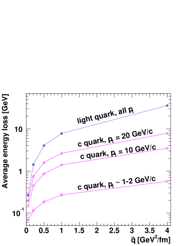
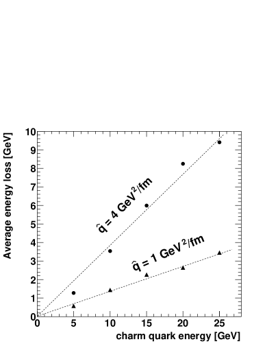
Figure 8.9: Left: average energy loss as function of the transport coefficient for light (massless) quarks and for charm ($m_{\rm c}=1.2\leavevmode\nobreak\ \mathrm{GeV}$) quarks with different transverse momenta. Right: average energy loss for charm quarks as a function of their energy; the dashed lines correspond to $\left\langle\Delta E\right\rangle\propto E$.

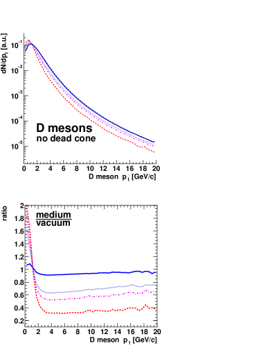
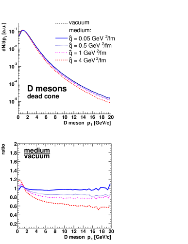
Figure 8.10: Transverse momentum distributions of D mesons in the vacuum and in the medium (upper panels) and medium-to-vacuum ratios (lower panels). The dead cone correction is not included in the left-side panels and included in the right-side panels.

The dead cone correction, in the form a simple factor $F_{\rm H/L}$ that multiplies the radiated gluon energy distribution d$I/$d$\omega$, can be directly implemented in the SW quenching weights as they are calculated in Ref. [51]. However, this way of proceeding would be much more CPU-expensive than the simple folding we outlined above and also non-rigorous from a theoretical point of view [102]. The results on the energy loss probability distribution obtained with the two methods, ‘folding $F_{\rm H/L}\otimes P(\Delta E)$’ and ‘$F_{\rm H/L}$ in the SW weights’, were compared for $\hat{q}=1\leavevmode\nobreak\ \mathrm{GeV}^{2}/\mathrm{fm}$, $L=5\leavevmode\nobreak\ \mathrm{fm}$, $m_{\rm c}=1.2\leavevmode\nobreak\ \mathrm{GeV}$ and $p_{\rm t}=10,\leavevmode\nobreak\ 20,\leavevmode\nobreak\ 30\leavevmode\nobreak\ \mathrm{GeV}/c$. The comparison for $p_{\rm t}=10\leavevmode\nobreak\ \mathrm{GeV}/c$, reported in Fig. 8.8 (right), is quite satisfactory. A similar agreement is found for $p_{\rm t}=20$ and $30\leavevmode\nobreak\ \mathrm{GeV}/c$.

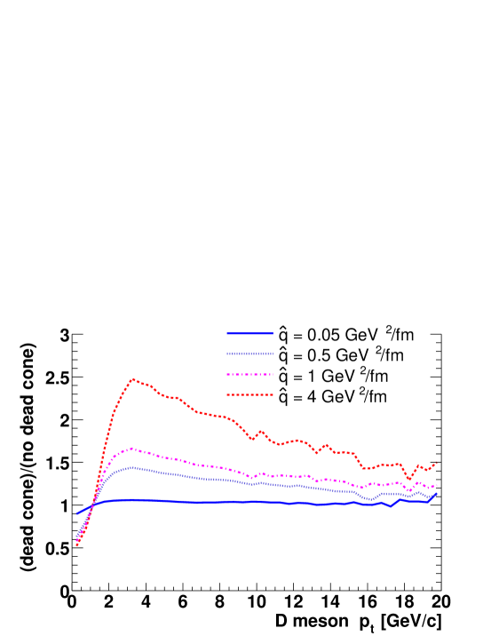
Figure 8.11: Ratio of the D mesons $p_{\rm t}$ distributions with and without dead cone effect.

Figure 8.9 (left) reports the average energy loss as a function of the transport coefficient for light quarks and for charm quarks with $p_{\rm t}=1$-$2,\leavevmode\nobreak\ 10,\leavevmode\nobreak\ 20\leavevmode\nobreak\ \mathrm{GeV}/c$, as obtained with the described dead cone correction ($p_{\rm t}$-dependent $P(\Delta E)\otimes F_{\rm H/L}$ folding). With $\hat{q}=4\leavevmode\nobreak\ \mathrm{GeV}^{2}/\mathrm{fm}$, for c quarks of $1$-$2,\leavevmode\nobreak\ 10,\leavevmode\nobreak\ 20\leavevmode\nobreak\ \mathrm{GeV}/c$ $\left\langle\Delta E\right\rangle$ is about 2%, 10% and 20%, respectively, of the average loss for massless quarks.

Remarkably, for charm quarks we find that, for given $\hat{q}$, the average energy loss is approximately proportional to the quark energy, $\left\langle\Delta E\right\rangle\propto E$, (see right panel of Fig. 8.9), while the BDMPS average energy loss for massless partons is independent of the parton energy. On the basis of this observation we expect that not only the magnitude but also the $p_{\rm t}$-dependence of the nuclear modification factor of D mesons will be significantly affected by the dead cone.

The transverse momentum distributions of charm mesons for $\hat{q}=0$ (vacuum), 0.05 (cold nuclear matter), 0.5, 1 and $4\leavevmode\nobreak\ \mathrm{GeV}^{2}/\mathrm{fm}$ are shown in Fig. 8.10 without (left) and with (right) dead cone correction. For $\hat{q}=4\leavevmode\nobreak\ \mathrm{GeV}^{2}/\mathrm{fm}$ the ratio medium/vacuum, also reported in the figure, is of order 0.3 and rather flat with $p_{\rm t}$ if the dead cone is not accounted for and it is of order 0.7-0.5, decreasing with $p_{\rm t}$, with the dead cone correction. For $p_{\rm t}<1\leavevmode\nobreak\ \mathrm{GeV}/c$, the ratio is larger than 1 due to the thermalized c quark component, which accumulates at low momenta.

In order to better quantify the effect of the dead cone we plot the ratio of the $p_{\rm t}$ distributions with and without the correction included in the quenching weights (Fig. 8.11). The ratio is clearly sensitive to the density of the medium, e.g $\simeq 2$-$2.5$ for $\hat{q}=4\leavevmode\nobreak\ \mathrm{GeV}^{2}/\mathrm{fm}$ and $\simeq 1.5$ for $\hat{q}=1\leavevmode\nobreak\ \mathrm{GeV}^{2}/\mathrm{fm}$, and it decreases with $p_{\rm t}$ as the mass of the charm quark becomes negligible. This (dead cone)/(no dead cone) ratio should be reflected by the the D/$hadrons$ observable, which we will calculate in the last section of the chapter.

8.3 Results (I): nuclear modification factor $R_{\rm AA}$ for ${\rm D}$ mesons

The nuclear modification factor for $\mathrm{D^{0}}$ mesons

$$R_{\rm AA}(p_{\rm t})=\frac{{\rm d}\sigma^{\rm AA}/{\rm d}p_{\rm t}/{\rm binary\leavevmode\nobreak\ NN\leavevmode\nobreak\ collision}}{{\rm d}\sigma^{\rm pp}/{\rm d}p_{\rm t}}$$ (8.4)

as obtained including only nuclear shadowing and intrinsic parton transverse momentum broadening and no parton energy loss, is shown in Fig. 8.12. The estimated error contributions reported in the figure are:

• statistical error, obtained by adding in quadrature the statistical errors estimated for Pb–Pb and for pp collisions (see Fig. 7.8); it amounts to 20% at $p_{\rm t}=1\leavevmode\nobreak\ \mathrm{GeV}/c$, 4% at $4\leavevmode\nobreak\ \mathrm{GeV}/c$ and 13% at $14\leavevmode\nobreak\ \mathrm{GeV}/c$;

• systematic error for MC corrections, 15%, from quadratic sum of Pb–Pb and pp contributions (see Fig. 7.8); we remind that this error has been conservatively set to 10%, but may well be lower;

• systematic error on centrality selection and nuclear parameters, $8\%\oplus 5\%=9.5\%$, discussed in Section 7.2.2; the nucleon–nucleon inelastic cross section uncertainty, which can be reasonably assumed to be the same for Pb–Pb and pp, cancels out in the ratio;

• systematic error on the extrapolation of the pp results from $14\leavevmode\nobreak\ \mathrm{TeV}$ to $5.5\leavevmode\nobreak\ \mathrm{TeV}$, 3-6% depending on $p_{\rm t}$, as shown in Fig. 7.13.

The systematic uncertainties on the ${\rm D^{0}\to K^{-}\pi^{+}}$ branching ratio and on the correction for feed-down from ${\rm B}\to\mbox{$\mathrm{D^{0}}$}+X$ decays (i.e. uncertainty on $\mathrm{b\overline{b}}$ cross section) can be assumed to be the same for the two colliding systems and neglected in the ratio.

Figure 8.12: Nuclear modification factor for $\mathrm{D^{0}}$ mesons. Nuclear shadowing and intrinsic $k_{\rm t}$ broadening are included. Energy loss is not included.

The effect of shadowing, introduced via the EKS98 parameterization [33], is visible as a suppression of $R_{\rm AA}$ at low transverse momenta, corresponding to small Bjorken $x$. As estimated in Section 2.2, the effect is negligible for $p_{\rm t}>6$-$7\leavevmode\nobreak\ \mathrm{GeV}/c$. Since there is significant uncertainty on the magnitude of shadowing in the low-$x$ region (see Fig. 1.13), we have studied the effect of such uncertainty on $R_{\rm AA}$ by varying the nuclear modification of parton distribution functions (PDFs). In Fig. 8.13 we show different modifications of the gluon PDF for Pb nuclei and $Q^{2}=5\leavevmode\nobreak\ \mathrm{GeV}^{2}\simeq(2\,m_{\rm c})^{2}$ —the valence and sea quark PDFs were changed accordingly— and the resulting $R_{\rm AA}$. Also in the case of shadowing 50% stronger than in EKS98 (curve labelled “c”), we find $R_{\rm AA}>0.93$ for $p_{\rm t}>7\leavevmode\nobreak\ \mathrm{GeV}/c$. We can, thus, confirm that for $p_{\rm t}>7\leavevmode\nobreak\ \mathrm{GeV}/c$ only (possible) parton energy loss is expected to affect the nuclear modification factor of D mesons.

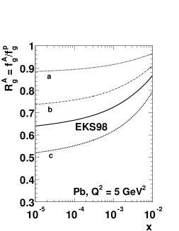
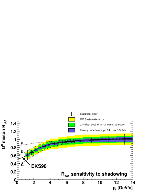
Figure 8.13: Nuclear modification of the gluon PDF (left) —the valence and sea quark PDFs were also changed accordingly— and its effect on $R_{\rm AA}$ of $\mathrm{D^{0}}$ mesons (right).

Figure 8.14 presents the nuclear modification factor in the vacuum and in the medium for different values of the transport coefficient. The result obtained without (with) dead cone is shown in the upper (lower) panel. All systematic uncertainties were added in quadrature.

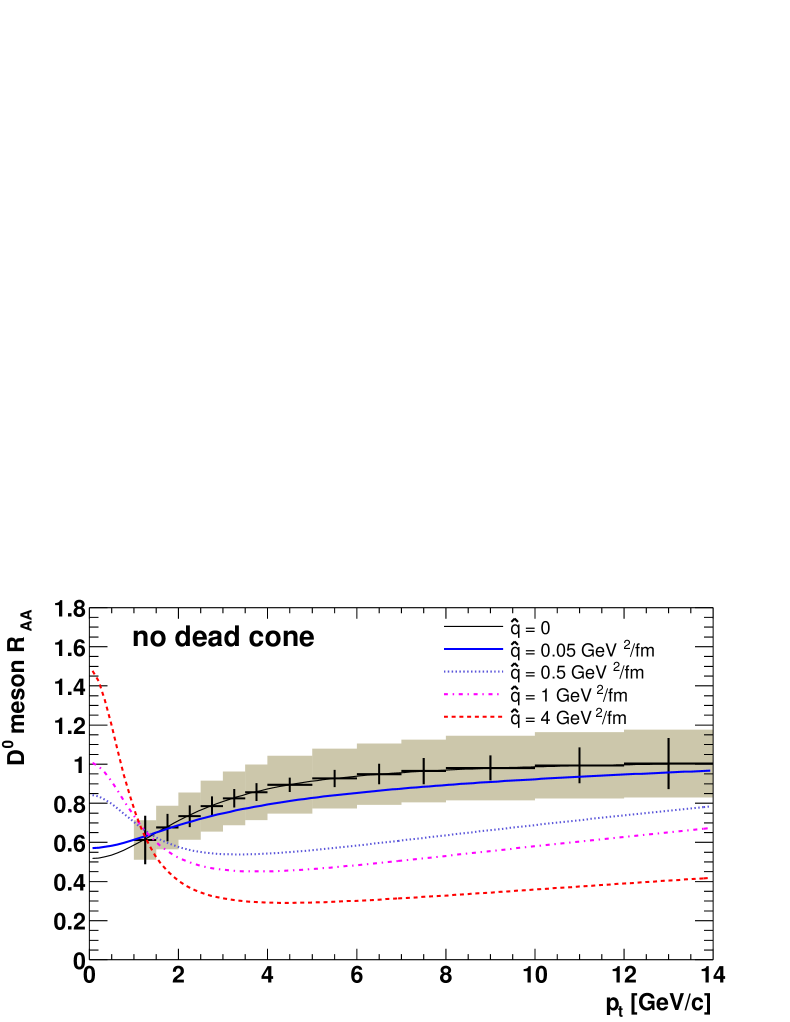
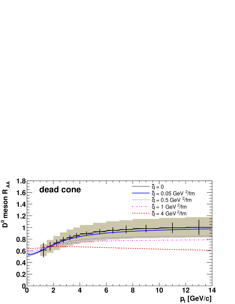
Figure 8.14: Nuclear modification factor for $\mathrm{D^{0}}$ mesons with shadowing, intrinsic $k_{\rm t}$ broadening and parton energy loss. Upper panel: without dead cone correction; lower panel: with dead cone correction. Errors corresponding to the curve for $\hat{q}=0$ are shown: bars = statistical, shaded area = systematic.

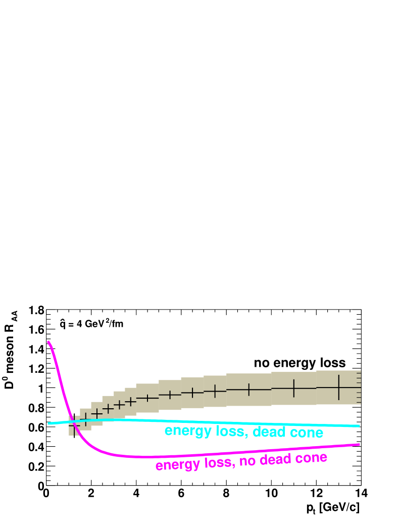
Figure 8.15: Nuclear modification factor for $\mathrm{D^{0}}$ mesons with shadowing, intrinsic $k_{\rm t}$ broadening and parton energy loss for $\hat{q}=4\leavevmode\nobreak\ \mathrm{GeV}^{2}/\mathrm{fm}$. Errors: bars = statistical, shaded area = systematic.

For $\hat{q}=4\leavevmode\nobreak\ \mathrm{GeV}^{2}/\mathrm{fm}$ and no dead cone, we find $R_{\rm AA}$ reduced, with respect to 1, by a factor about 3 and slightly increasing with $p_{\rm t}$, from 0.3 at $6\leavevmode\nobreak\ \mathrm{GeV}/c$ to 0.4 at $14\leavevmode\nobreak\ \mathrm{GeV}/c$. Even for a transport coefficient lower by a factor 4, $\hat{q}=1\leavevmode\nobreak\ \mathrm{GeV}^{2}/\mathrm{fm}$, $R_{\rm AA}$ is significantly reduced (0.5-0.6). When the dead cone effect is taken into account, the $R_{\rm AA}$ reduction due to quenching is found to be lower by about a factor 1.5-2.5, depending on $\hat{q}$ and $p_{\rm t}$, as already seen in Fig. 8.11. For our reference transport coefficient, $4\leavevmode\nobreak\ \mathrm{GeV}^{2}/\mathrm{fm}$, $R_{\rm AA}$ with dead cone is equal to 0.6 and essentially flat as a function of $p_{\rm t}$. The expectations without and with dead cone are compared directly in Fig. 8.15, for $\hat{q}=4\leavevmode\nobreak\ \mathrm{GeV}^{2}/\mathrm{fm}$.

We point out that the different $p_{\rm t}$ dependence appears to be the only distinctive feature between a scenario with moderate quenching and negligible dead cone effect (e.g. $\hat{q}=1\leavevmode\nobreak\ \mathrm{GeV}^{2}/\mathrm{fm}$ in the upper panel of Fig. 8.14) and a scenario with large quenching but also strong dead cone effect (e.g. $\hat{q}=4\leavevmode\nobreak\ \mathrm{GeV}^{2}/\mathrm{fm}$ in the lower panel). However, the estimated systematic uncertainty of about 18% may prevent from giving a clear statement on the $p_{\rm t}$ dependence of $R_{\rm AA}$. As remarked in Chapter 2, the comparison of the quenching of charm-quark-originated mesons and massless-parton-originated hadrons will be the best suited tool to disentangle the relative importance of energy loss and dead cone effects.

Before moving to the results on the D/$hadrons$ ratio, we shortly comment on the errors presented in Figs. 8.14 and 8.15. The relative systematic error ($\simeq 18\%$) is larger than the statistical error up to $p_{\rm t}=14\leavevmode\nobreak\ \mathrm{GeV}/c$ for $\hat{q}=0$. However, as $\hat{q}$ is increased the statistics $S$ of $\mathrm{D^{0}}$ mesons at large transverse momenta in Pb–Pb collisions decreases. Consequently, the relative statistical error increases roughly as $1/\sqrt{S}$. For example, for $\hat{q}=4\leavevmode\nobreak\ \mathrm{GeV}^{2}/\mathrm{fm}$ and no dead cone effect the factor 3 reduction in $R_{\rm AA}$ is accompanied by an increase of a factor $\approx\sqrt{3}$ in the statistical error, which becomes larger than the systematic one at high $p_{\rm t}$. Due to the lower quenching, the effect is less important if the dead cone is included.

8.4 Results (II): ${\rm D}/hadrons$ ratio

For the comparison of energy loss of heavy quarks and of massless partons, we consider the ratio ($\mathrm{D^{0}}$ mesons)/(charged hadrons), hereafter indicated as D/$h$, rather than the ratio ($\mathrm{D^{0}}$ mesons)/(pions), the reason being that the former can be measured with smaller systematic uncertainty. Experimentally, the $\mathrm{D^{0}}$-to-pions ratio can be defined up to $p_{\rm t}\simeq 15\leavevmode\nobreak\ \mathrm{GeV}/c$ only using neutral pions, which decay as $\pi^{0}\to\gamma\gamma$ and can be identified by means of invariant mass analysis of pairs of photons reconstructed in an electro-magnetic calorimeter (e.g. PHOS). However, this would not allow to cancel out the ‘MC systematic uncertainties’ of the $\mathrm{D^{0}}$ and $\pi^{0}$ $p_{\rm t}$ distributions, because they are measured using different detectors that have different systematics. On the other hand, the use of unidentified charged hadrons reconstructed by tracking in TPC and ITS allows to partially cancel out the uncertainties introduced by acceptance and efficiency corrections of these detectors. Part of the error will still remain as each $\mathrm{D^{0}}$ is reconstructed as a pair of opposite-charge tracks, while a charged hadron is obviously only one track.

The D/$h$ ratio, defined as

$$R_{{\rm D}/h}(p_{\rm t})=\frac{R_{\rm AA}^{\rm D^{0}}(p_{\rm t})}{R_{\rm AA}^{h}(p_{\rm t})}=\frac{{\rm d}\sigma^{\rm AA}(\mbox{$\mathrm{D^{0}}$})/{\rm d}p_{\rm t}}{{\rm d}\sigma^{\rm pp}(\mbox{$\mathrm{D^{0}}$})/{\rm d}p_{\rm t}}\times\frac{{\rm d}\sigma^{\rm pp}(h)/{\rm d}p_{\rm t}}{{\rm d}\sigma^{\rm AA}(h)/{\rm d}p_{\rm t}},$$ (8.5)

is presented in Fig. 8.16 for the range $5<p_{\rm t}<14\leavevmode\nobreak\ \mathrm{GeV}/c$. We used $R_{\rm AA}^{h}$ for hadrons as reported in the left panel of Fig. 8.5 and $R_{\rm AA}^{\rm D^{0}}$ for $\mathrm{D^{0}}$ mesons, without and with dead cone, as reported in Fig. 8.14.

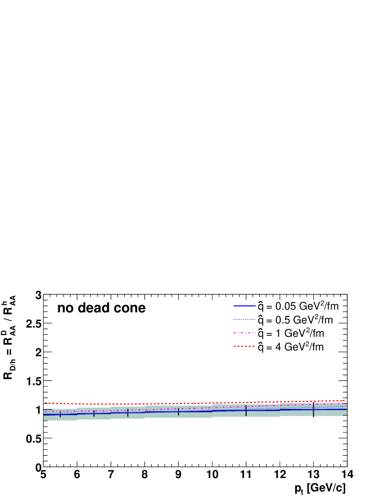
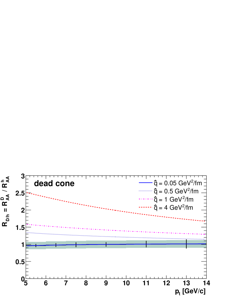
Figure 8.16: Ratio of the nuclear modification factors for $\mathrm{D^{0}}$ mesons and for charged hadrons. Upper panel: without dead cone correction; lower panel: with dead cone correction. Errors corresponding to the curve for $\hat{q}=0.05\leavevmode\nobreak\ \mathrm{GeV}^{2}/\mathrm{fm}$ are shown: bars = statistical, shaded area = systematic.

The estimated errors on $R_{{\rm D}/h}$ are:

• statistical error; the same as for $R_{\rm AA}^{\rm D^{0}}$, since the statistical error on the $p_{\rm t}$ distributions of charged hadrons will be negligible for $p_{\rm t}<14\leavevmode\nobreak\ \mathrm{GeV}/c$;

• systematic error for MC corrections; this error partially cancels out in the two ratios $({\rm d}\sigma^{\rm AA}(\mbox{$\mathrm{D^{0}}$})/{\rm d}p_{\rm t})/({\rm d}\sigma^{\rm AA}(h)/{\rm d}p_{\rm t})$ and $({\rm d}\sigma^{\rm pp}(\mbox{$\mathrm{D^{0}}$})/{\rm d}p_{\rm t})/({\rm d}\sigma^{\rm pp}(h)/{\rm d}p_{\rm t})$; we consider a residual error of 10%, due to fact that $\mathrm{D^{0}}$ is two tracks while $h$ is one track.

• systematic error on the extrapolation of pp results from $14\leavevmode\nobreak\ \mathrm{TeV}$ to $5.5\leavevmode\nobreak\ \mathrm{TeV}$; both the $\mathrm{D^{0}}$ and the $h$ $p_{\rm t}$ distributions measured in pp collisions will have to be extrapolated to $5.5\leavevmode\nobreak\ \mathrm{TeV}$ by means of pQCD; we assume a $p_{\rm t}$-independent error of 5% on $R_{{\rm D}/h}$, slightly lower than what used for $R_{\rm AA}^{\rm D^{0}}$, considering that the pQCD uncertainties for $\mathrm{D^{0}}$ and for $h$ will be partially correlated.

The errors on the centrality selection in Pb–Pb cancel out because the $\mathrm{D^{0}}$ and $h$ analyses will be performed on the same sample of events. The total systematic error is $10\%\oplus 5\%\simeq 11\%$ and it is shown by the shaded bands in Fig. 8.16.

We find that, if the dead cone correction for c quarks is not included, $R_{{\rm D}/h}$ is essentially 1 in the considered $p_{\rm t}$ range, independently of the value of the transport coefficient, i.e. of the magnitude of the energy loss effect. When the dead cone is taken into account, $R_{{\rm D}/h}$ is enhanced of a factor strongly dependent on the transport coefficient of the medium: e.g. 2-2.5 for $\hat{q}=4\leavevmode\nobreak\ \mathrm{GeV}^{2}/\mathrm{fm}$ and 1.5 for $\hat{q}=1\leavevmode\nobreak\ \mathrm{GeV}^{2}/\mathrm{fm}$. The enhancement is decreasing with $p_{\rm t}$, as expected.

The $R_{{\rm D}/h}$ ratio is, therefore, found to be enhanced, with respect to 1, only by the dead cone effect and, consequently, it appears as a very clean tool to investigate and quantify this effect. We point out that the obtained $R_{{\rm D}/h}$ with dead cone is extremely similar to the ratio of the $\mathrm{D^{0}}$ transverse momentum distributions with and without dead cone, shown in Fig. 8.11.

In Section 2.3.3 we discussed how the D/$h$ ratio should, in principle, be enhanced also in absence of dead cone effect, as a consequence of the larger energy loss of gluons with respect to quarks. Such enhancement is essentially not observed in the obtained $R_{{\rm D}/h}$ because it is ‘compensated’ by the harder fragmentation of charm quarks with respect to light quarks and, particularly, gluons. With $z$ the typical momentum fraction taken by the hadron in the fragmentation, $p_{\rm t}^{\rm hadron}=z\,p_{\rm t}^{\rm parton}$, and $\Delta E$ the average energy loss for the parton, $(p_{\rm t}^{\rm parton})^{\prime}=p_{\rm t}^{\rm parton}-\Delta E$, we have

$$(p_{\rm t}^{\rm hadron})^{\prime}=p_{\rm t}^{\rm hadron}-z\,\Delta E,$$ (8.6)

meaning that the energy loss observed in the nuclear modification factor is, indeed, $z\,\Delta E$. We have, thus, to compare $z_{\rm c\to D}\,\Delta E_{\rm c}$ to $z_{\rm gluon\to hadron}\,\Delta E_{\rm gluon}$. With $z_{\rm gluon\to hadron}\approx 0.4$ (from Fig. 8.3, left), $z_{\rm c\to D}\approx 0.8$ for $p_{\rm t}^{\rm D}>5\leavevmode\nobreak\ \mathrm{GeV}/c$ (it is $\approx 0.75$ for $p_{\rm t}^{\rm D}>0$, see Section 3.5) and $\Delta E_{\rm c}=\Delta E_{\rm gluon}/2.25$ (without dead cone), we obtain

$$z_{\rm c\to D}\,\Delta E_{\rm c}\approx 0.9\,z_{\rm gluon\to hadron}\,\Delta E_{\rm gluon}.$$ (8.7)

This simple estimate confirms that the quenching for D mesons is almost the same as for (non-charm) charged hadrons, if the dead cone effect is not considered.

The errors reported in Fig. 8.16 show that ALICE is expected to have good capabilities for the study of $R_{{\rm D}/h}$: in the range $5<p_{\rm t}<10\leavevmode\nobreak\ \mathrm{GeV}/c$ the enhancement due to the dead cone is an effect of more than $3\leavevmode\nobreak\ \sigma$ for $\hat{q}>1\leavevmode\nobreak\ \mathrm{GeV}^{2}/\mathrm{fm}$. The comparison of the values for the transport coefficient extracted from the nuclear modification factor of charged hadrons (or neutral pions) and, independently, from the D/$hadrons$ ratio shall provide an important test for the coherence of our understanding of the energy loss of hard probes propagating in the dense QCD medium formed in Pb–Pb collisions at the LHC.

In conclusion, we remark that, presently, the procedure we used and equivalent ones [103] are the only way to keep into account (though with an approximation) the predicted dead cone effect in a simulation of energy loss. This topic now attracts more and more attention from the theoretical side and many of the present uncertainties should be reduced in the near future. These developments will be deployed to improve our studies.

Conclusions

This work was aimed at studying the performance of the ALICE detector for measuring charm production in heavy ion collisions at the LHC and for investigating the properties of the deconfined quark–gluon medium formed in central nucleus–nucleus reactions by a comparison of its ‘opacities’ to massive (charm) quarks and massless partons.

We carried out a detailed simulation study for the detection of $\mathrm{D^{0}}$ mesons in the $\rm K\pi$ decay channel in central Pb–Pb at $\sqrt{s_{\scriptscriptstyle{{\rm NN}}}}=5.5\leavevmode\nobreak\ \mathrm{TeV}$ and pp collisions at $\sqrt{s}=14\leavevmode\nobreak\ \mathrm{TeV}$. The detection strategy is based on the invariant mass analysis of fully reconstructed topologies originated in displaced secondary decay vertices. This strategy exploits the excellent capabilities of the ALICE detector in track reconstruction, vertexing and particle identification. The signal selection was studied as a function of the transverse momentum $p_{\rm t}$.

The $p_{\rm t}$-differential $\mathrm{D^{0}}$ production cross section can be measured in the range $1$-$14\leavevmode\nobreak\ \mathrm{GeV}/c$ for Pb–Pb and $0$-$14\leavevmode\nobreak\ \mathrm{GeV}/c$ for pp collisions with statistical uncertainty better than $10$-$15\%$ and systematic uncertainty better than $15$-$20\%$.

The effect of parton energy loss in a high-opacity quark–gluon medium was simulated using a state-of-the-art calculation. Particular attention was devoted to the description of the collision geometry and, thus, of the path length traveled by fast partons in the medium. We found that the use of an equivalent average length is not a good solution and can significantly bias the final results. We implemented a simulation chain that allows to include an algorithm accounting for the suppression of small-angle gluon radiation off massive quarks (dead cone effect). This enabled us to obtain and compare the quenched $p_{\rm t}$ distributions of c quarks and D mesons, with and without dead cone effect. With the medium density estimated on the basis of the hadron quenching measured at RHIC, D meson production in the range $3<p_{\rm t}<15\leavevmode\nobreak\ \mathrm{GeV}/c$ in central Pb–Pb collisions is expected to be suppressed by a factor 3, with respect to binary scaling from pp collisions, if the dead cone is not included and by a factor 1.5 if it is included.

The dead cone effect can be studied by means of the D/$charged\leavevmode\nobreak\ hadrons$ ratio. This ratio is found to be enhanced, with respect to 1, only by the dead cone effect and the enhancement, which is sensitive to the density of the medium, may reach up to a factor 2-2.5 for the conditions expected at the LHC.

Remarkably, we find that D/$charged\leavevmode\nobreak\ hadrons$ is essentially 1, independently of $p_{\rm t}$, if the dead cone is not included. The expected enhancement due to the larger energy loss for gluons, that generate most of the hadrons, than for (c) quarks, that generate D mesons, is not observed. This is explained by the softer fragmentation of gluons with respect to charm quarks.

We identified a range in transverse momentum, $7<p_{\rm t}<14\leavevmode\nobreak\ \mathrm{GeV}/c$, where energy loss studies can be experimentally addressed using reconstructed ${\rm D^{0}\to K^{-}\pi^{+}}$ decays. In fact, we showed that the other nuclear effects (shadowing and intrinsic parton $p_{\rm t}$ broadening) should be limited to the region $p_{\rm t}<7\leavevmode\nobreak\ \mathrm{GeV}/c$.

The estimated experimental uncertainties allow to conclude that ALICE has a good potential for studying, for gluons, light quarks and heavy quarks, the medium-induced energy loss effect, which is one of the main predictions of QCD in hot and dense matter.

In order to fully exploit such excellent physics reach, it is now important to proceed with the preparation of the tools for data analysis and, in parallel, to push further the physics feasibility studies, in close collaboration with the theoretical community. The most promising and stimulating items emerged during this work are in the direction of parton energy loss.

Appendix A Kinematics of the ${\rm D^{0}\to K^{-}\pi^{+}}$ decay

In this appendix we consider the kinematics of the two-body decay ${\rm D^{0}\to K^{-}\pi^{+}}$; in particular, we show how the experimental resolution on the invariant mass is proportional to the momentum resolution and we calculate the mean value of the impact parameter of the decay products.  

For two particles with four-momenta $(E_{1},\vec{p}_{1})$ and $(E_{2},\vec{p}_{2})$, the invariant mass is defined as the modulus of the total four-momentum:

$$M=\sqrt{s_{12}}=\sqrt{(E_{1}+E_{2})^{2}-(\vec{p}_{1}+\vec{p}_{2})^{2}}.$$ (A.1)

In the case of the ${\rm D^{0}\to K^{-}\pi^{+}}$ decay, the invariant mass of the $\mbox{$\mathrm{K}$}\pi$ system is equal to the $\mathrm{D^{0}}$ mass.

In the relativistic case, $E\simeq p$, we can write:

$$M^{2}\simeq(p_{\rm K}+p_{\pi})^{2}-(\vec{p}_{\rm K}+\vec{p}_{\pi})^{2}=2\,p_{\rm K}\,p_{\pi}\,(1-\cos\psi_{\rm K\pi}),$$ (A.2)

where $\psi_{\rm K\pi}$ is the angle between the two particles. Since the angles are usually measured with much better precision than the momenta (in particular in a moderate magnetic field, as is the case in ALICE), the main contribution to the invariant mass resolution comes from the momentum resolution. By differentiation of the previous expression, we obtain:

$$\frac{\Delta M}{M}=\frac{1}{\sqrt{2}}\,\frac{\Delta p}{p}.$$ (A.3)

This relation holds with good approximation for $\mathrm{D^{0}}$ meson decays at the LHC, since the two decay products can be considered relativistic (Section 3.5).

In the rest frame of the $\mathrm{D^{0}}$ meson, the two decay products are emitted back-to-back with the same total momentum $p^{\star}$ and with energies $E_{\rm K}^{\star}=\sqrt{m_{\rm K}^{2}+(p^{\star})^{2}}$ and $E_{\pi}^{\star}=\sqrt{m_{\pi}^{2}+(p^{\star})^{2}}$. Since $\vec{p}^{\star}_{\rm K}=-\vec{p}^{\star}_{\pi}$, the expression of the invariant mass gives:

$$M_{\rm D^{0}}=E_{\rm K}^{\star}+E_{\pi}^{\star}.$$ (A.4)

Using this relation and the masses of the involved particles [60], the values $p^{\star}=0.86\leavevmode\nobreak\ \mathrm{GeV}/c$, $E^{\star}_{\rm K}=0.99\leavevmode\nobreak\ \mathrm{GeV}/c$ and $E^{\star}_{\pi}=0.87\leavevmode\nobreak\ \mathrm{GeV}/c$ are obtained. We introduce the decay angle $\theta^{\star}$, defined as the angle, in the $\mathrm{D^{0}}$ rest frame, between the direction of the momenta of the decay products and the $\mathrm{D^{0}}$ flight direction (see sketch in Fig. A.1, left). The momenta of the two particles can be decomposed in a component perpendicular to the $\mathrm{D^{0}}$ flight direction, $q_{\rm t}^{\star}=p^{\star}\sin\theta^{\star}$, and one parallel to it, $q_{\rm l}^{\star}=\pm p^{\star}\cos\theta^{\star}$.

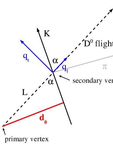
Figure A.1: Left: definition of the decay angle $\theta^{\star}$ in the $\mathrm{D^{0}}$ reference frame. Right: decay topology with the impact parameter $d_{0}$.

In the global reference frame, where the $\mathrm{D^{0}}$ has a velocity $\beta c$, the momentum of the generic decay product, decomposed with respect to the $\mathrm{D^{0}}$ flight direction, is:

$$p=\sqrt{q_{\rm t}^{2}+q_{\rm l}^{2}},$$ (A.5)

where:

$$q_{\rm t}=q_{\rm t}^{\star}\leavevmode\nobreak\ \leavevmode\nobreak\ \leavevmode\nobreak\ {\rm and}\leavevmode\nobreak\ \leavevmode\nobreak\ \leavevmode\nobreak\ q_{\rm l}=\gamma(q_{\rm l}^{\star}+\beta E^{\star}),$$ (A.6)

having applied the Lorentz boost to the component along the $\mathrm{D^{0}}$ flight direction. We remark that, since $E^{\star}_{\rm K}>E^{\star}_{\pi}$, the kaon has, on average, a momentum larger than that of the pion.

Let us now calculate the value of the impact parameter projection on the bending plane, that we indicate here as $d_{0}$. With reference to the sketch in Fig. A.1 (right), we have:

$$d_{0}=L\,\sin\alpha,$$ (A.7)

where $L=ct\beta\gamma$ is the decay length of a $\mathrm{D^{0}}$ with proper decay time $t$, and $\alpha$ is the angle of the considered decay particle with respect to the $\mathrm{D^{0}}$ flight-direction. The effect of the magnetic field, $B$, can be neglected because, for $B=0.4\leavevmode\nobreak\$T and $p_{\rm t}^{\rm K,\pi}=1\leavevmode\nobreak\ \mathrm{GeV}/c$, the sagitta of the arc with length $\ell=100\leavevmode\nobreak\ \mathrm{\mu m}$ (the typical value of $L$) is $s=0.3B\ell^{2}/8p_{\rm t}\simeq 10^{-4}\leavevmode\nobreak\ \mathrm{\mu m}$.

The ‘detectable’ decays are those with large impact parameter Therefore, for this estimation, we consider the situation in which the decay plane coincides with the bending plane and the decay angle $\theta^{\star}$ is $\pi/2$. This is the configuration with higher probability to be detected.

With this assumption we have:

$$\sin\alpha=\frac{q_{\rm t}}{\sqrt{q_{\rm t}^{2}+q_{\rm l}^{2}}}=1\Bigg{/}{\sqrt{1+\left(\frac{q_{\rm l}}{q_{\rm t}}\right)^{2}}}.$$ (A.8)

Then, using $p^{\star}\simeq E^{\star}$ and $\theta^{\star}=\pi/2$, we have:

$$\frac{q_{\rm l}}{q_{\rm t}}=\frac{\gamma(p^{\star}\cos\theta^{\star}+\beta E^{\star})}{p^{\star}\sin\theta^{\star}}\simeq\frac{\beta\,\gamma\,p^{\star}}{p^{\star}}=\beta\,\gamma.$$ (A.9)

We now write the impact parameter as

$$d_{0}=ct\,\beta\,\gamma\Bigg{/}{\sqrt{1+(\beta\,\gamma)^{2}}}=ct\Bigg{/}{\sqrt{1+1/(\beta\,\gamma)^{2}}}=ct\Bigg{/}{\sqrt{1+(M_{\rm D^{0}}/p_{\rm D^{0}})^{2}}}.$$ (A.10)

Following the exponential distributions of the proper decay time $t$, the impact parameter has an exponential distribution with mean value:

$$\left\langle d_{0}\right\rangle=c\tau\Bigg{/}{\sqrt{1+(M_{\rm D^{0}}/p_{\rm D^{0}})^{2}}}=124\leavevmode\nobreak\ \mathrm{\mu m}\Bigg{/}{\sqrt{1+(M_{\rm D^{0}}/p_{\rm D^{0}})^{2}}}.$$ (A.11)

In Fig. A.2 we plot the mean value of $d_{0}$ as a function of the momentum of the $\mathrm{D^{0}}$. The value (marked by the arrows) corresponding to the average momentum of $\mathrm{D^{0}}$ mesons with $|y|<1$ is $\approx 105\leavevmode\nobreak\ \mathrm{\mu m}$. For momenta of $\sim 1\leavevmode\nobreak\ \mathrm{GeV}/c$, the average impact parameter is very small; therefore, in these cases, only mesons that decay with proper decay time $t$ significantly larger than the mean lifetime $\tau$ can be identified by means of a displaced vertex selection.

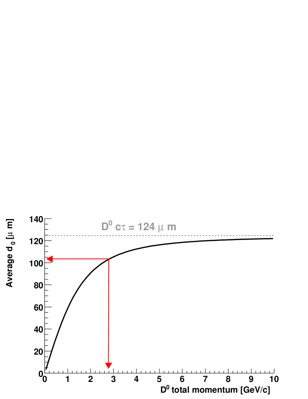
Figure A.2: Average impact parameter in the transverse plane for the decay products of a $\mathrm{D^{0}}$ meson, as a function of its momentum. The arrows mark the value corresponding to the average momentum of $\mathrm{D^{0}}$ mesons with $|y|<1$ at LHC energies.

Appendix B PYTHIA parameters used for heavy quark generation at LHC energies

In Table B.1 we report the complete list of parameters used in the PYTHIA event generator [57] in order to reproduce the inclusive $p_{\rm t}$ distribution for the heavy quarks given by the HVQMNR program based on NLO calculations by M. Mangano, P. Nason and G. Ridolfi [64]. A detailed description of the parameters can be found in Ref. [57].

As specified in Section 3.4, the main parameter we tuned is the lower $p_{\rm t}^{\rm hard}$ limit: the optimal value was found to be $2.1\leavevmode\nobreak\ \mathrm{GeV}/c$ for charm production and $2.75\leavevmode\nobreak\ \mathrm{GeV}/c$ for beauty production, both for Pb–Pb collisions at $\sqrt{s_{\scriptscriptstyle{{\rm NN}}}}=5.5\leavevmode\nobreak\ \mathrm{TeV}$ and for pp collisions at $\sqrt{s}=14\leavevmode\nobreak\ \mathrm{TeV}$. Therefore, one can reasonably assume that the same values can be used also for p–Pb collisions at $\sqrt{s_{\scriptscriptstyle{{\rm NN}}}}=8.8\leavevmode\nobreak\ \mathrm{TeV}$.

The different values for the partonic intrinsic transverse momentum $k_{\rm t}$ in pp, p–Pb and Pb–Pb collisions were taken from Ref. [36].

Table B.1: PYTHIA parameters used for the generation of charm and beauty quarks in pp collisions at 14 TeV, p–Pb collisions at 8.8 TeV and Pb–Pb collisions at 5.5 TeV. All non-specified parameters are left to PYTHIA 6.150 defaults.

Description	Parameter	Charm	Beauty
Process types	MSEL	1	1
Quark mass $[\mathrm{GeV}]$	PMAS(4/5,1)	1.2	4.75
Minimum $p_{\rm t}^{\rm hard}\leavevmode\nobreak\ [\mathrm{GeV}/c]$	CKIN(3)	2.1	2.75
CTEQ4L	MSTP(51)	4032	4032
Proton PDF	MSTP(52)	2	2
Switch off	MSTP(81)	0	0
multiple	PARP(81)	0	0
interactions	PARP(82)	0	0
Initial/Final parton	MSTP(61)	1	1
shower on	MSTP(71)	1	1
2nd order $\alpha_{s}$	MSTP(2)	2	2
QCD scales	MSTP(32)	2	2
for hard scattering	PARP(34)	1	1
and parton shower	PARP(67)	1	1
	PARP(71)	4	1
Intrinsic $k_{\rm t}$
from gaussian distr. with mean 0	MSTP(91)	1	1
$\sigma$ $[\mathrm{GeV}/c]$	PARP(91)	1.00 (pp)	1.00 (pp)
		1.16 (p–Pb)	1.60 (p–Pb)
		1.30 (Pb–Pb)	2.04 (Pb–Pb)
upper cut-off (at 5 $\sigma$) $[\mathrm{GeV}/c]$	PARP(93)	5.00 (pp)	5.00 (pp)
		5.81 (p–Pb)	8.02 (p–Pb)
		6.52 (Pb–Pb)	10.17 (Pb–Pb)

Appendix C Parameterization of the TPC tracking response: validation tests

This appendix is an extract from:
A. Dainese and N. Carrer, ALICE Internal Note ALICE-INT-2003-011 (2003).

After defining the track parameters used in the TPC, we report the results of the tests that were performed in order to validate the parameterization tool for the use in physics studies. Refer to the complete note [85] for details on the implementation of the method.

C.1 Description of the track parameters used in the TPC

We remind that the ALICE TPC is a cylinder shell with inner and outer radii of $\approx 85\leavevmode\nobreak\ \mathrm{cm}$ and $\approx 250\leavevmode\nobreak\ \mathrm{cm}$, respectively, and length of $\approx 500\leavevmode\nobreak\ \mathrm{cm}$. The read-out planes are azimuthally segmented in 18 sectors, covering an angle of $20^{\circ}$ each. At the inner radius every sector is $30\leavevmode\nobreak\ \mathrm{cm}$ ($\simeq 85\leavevmode\nobreak\ \mathrm{cm}\times\tan 20^{\circ}$) wide. The non-active region between two adjacent sectors is approximately $2.7\leavevmode\nobreak\ \mathrm{cm}$ wide.

The ALICE global reference frame has the $z$ axis parallel to the beam line, and the $x$ and $y$ axes in the transverse plane, horizontal and vertical respectively. During track reconstruction, the helix track model is defined in the local reference frame obtained from the global one with a rotation around the $z$ axis:

$$\begin{array}[]{l}X=x\cdot\cos\alpha+y\cdot\sin\alpha\\ Y=-x\cdot\sin\alpha+y\cdot\cos\alpha\\ Z=z\end{array}$$ (C.1)

being $\alpha$ the azimuthal angle (w.r.t. the $x$ axis) of the TPC sector in which the track lies. Thus, $X$ is the radial coordinate in the sector. The track parameters are given at a reference plane for $X=X_{\rm ref}$.

The five track parameters are:

• $Y$: local $y$ coordinate of the track at the reference plane $X=X_{\rm ref}$;

• $Z$: local $z$ coordinate of the track at the reference plane $X=X_{\rm ref}$;

• $k$: track curvature. $k=1/R$, where $R$ is the radius of the circle obtained projecting the track on the bending plane;

• $\gamma$: $k\cdot X_{0}$, being $X_{0}$ the local $x$ coordinate of the centre of the circle on the bending plane;

• $\tan\lambda$: tangent of the track angle with the bending plane ($\tan\lambda=p_{z}/p_{\rm t}$).

C.2 Validation tests and results

In this section we present a comparison of the performances of the track reconstruction using:

• standard Kalman filter reconstruction in the TPC and in the ITS;

• parameterization of the tracking in the TPC and standard Kalman filter in the ITS.

We compare tracking efficiency and resolution on the track parameters. At the end of the section we report the gain in CPU time and disk space obtained performing the simulation with the parameterization tool we have implemented.

C.2.1 Tracking efficiency in the TPC and in the ITS

We start with a comparison of the total number of tracks found in the TPC: when using the parameterization this number is lower by $15$-$16\%$ than the number obtained with standard reconstruction. The loss has two sources:

1. With the standard reconstruction we get about $2$-$3\%$ of fake tracks in the TPC —a track is defined as fake if it has more than $10\%$ of incorrectly assigned clusters, typically the decay product of a particle that decays inside the TPC can originate a fake track (e.g. a charged pion from $\rm K_{S}^{0}\to\pi^{+}\pi^{-}$). Clearly, the parameterization will not give these tracks.

2. Tracks that enter the TPC in a non-active region (between two adjacent sectors) are not given by the parameterization, as they do not have a hit in the inner pad row. Nevertheless, a part of them can then leave signal on a sufficient number of pad rows and be reconstructed by the Kalman filter. For this reason, using the parameterization we have a loss that amounts to about $12\%$. In Fig. C.1 we plot the entrance position, in the local coordinates $(Y,\,Z)$, of the tracks that are reconstructed by the Kalman filter and not given by the parameterization. They are concentrated at the edge of the TPC sectors, for $|Y|\simeq 15\ \mathrm{cm}$. Recently, the simulation software was modified in order to allow to retrieve these tracks with the parameterization, but such change did not became available on time to be used for the studies presented in this thesis.

The lower ‘tracking efficiency’ in the TPC introduced by the parameterization does not limit the usefulness of the tool as, in principle, a correction could be applied. However, we chose not to apply such a correction and use the effect as a safety factor for the results of our simulation studies.

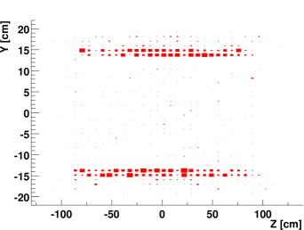
Figure C.1: Entering position the TPC sector for the tracks found by the Kalman filter and not given by the parameterization: they are concentrated at the edges of the sector.

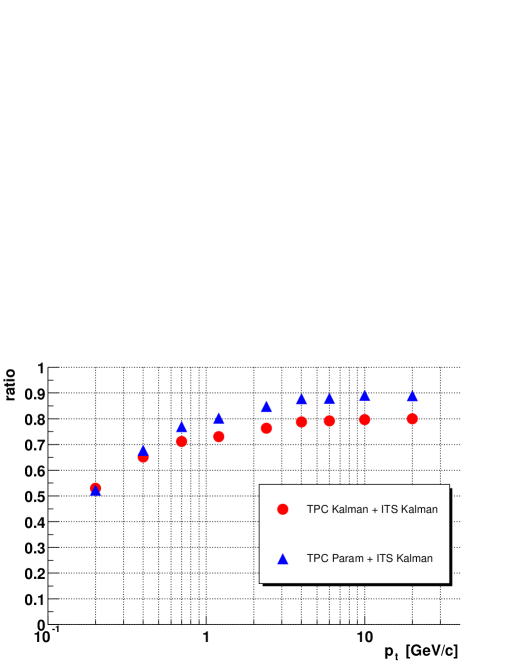
Figure C.2: Ratio of the number of TPC tracks prolonged in the ITS to the total number of tracks found in the TPC (circles: Kalman filter in the TPC, triangles: parameterization in the TPC).

The next step is the comparison of the tracking efficiency in the ITS, defined as the ratio of the number of TPC tracks prolonged in the ITS to the total number of tracks found in the TPC. In this way we can understand if the performance of the Kalman filter in the ITS is altered by the fact of using the parameterization for the TPC. Track reconstruction in the ITS was performed with the standard requirement of having one assigned cluster in each of the 6 layers. Only pions coming from the primary vertex were used for the comparison. The result is presented in Fig. C.2: the overall agreement is quite satisfactory; the slightly higher efficiency found when using the parameterization in the TPC is probably due to the fact that with the parameterization we do not have ‘low quality’ tracks (e.g. fake tracks or tracks that do not have hits in the inner pad rows of the TPC).

C.2.2 Resolution on the track parameters in TPC–ITS

In Fig. C.3 we report the comparison of the resolutions on the main track parameters, $p_{\rm t},\ p_{z},\ \tan\lambda,\ d_{0}(r\phi)$, after the reconstruction in the ITS. For all of these parameters we find that, using the parameterization of the tracking in the TPC, we reproduce the resolutions given by the standard reconstruction. Therefore, we conclude that the tool is suitable to be used for the simulation and analysis of physics cases.

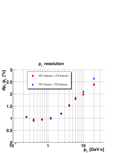
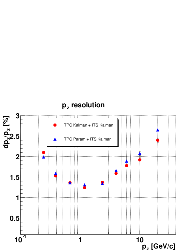
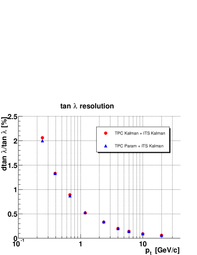
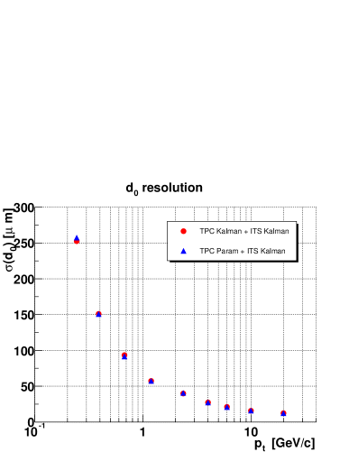
Figure C.3: Comparison of the resolution on the main track parameters (circles: Kalman filter in the TPC, triangles: parameterization in the TPC).

C.2.3 Effect on the required computing resources

The CPU time and disk space required for the simulation of an event with 6000 charged particles per unit of rapidity are reported in Table C.1 (only particles in the rapidity interval $|y|<2$ were transported through the detector). The reduction factor achieved with the introduction of the TPC tracking parameterization is 35.

The tool was integrated in the AliRoot [76] framework (class AliTPCtrackerParam).

Table C.1: CPU time (on a 800 MHz PC) and disk space for 1 central Pb–Pb collision (${\rm d}N_{\rm ch}/{\rm d}y=6000$), with particle transport restricted to the rapidity interval $|y|<2$.

		Full simulation and	Full simulation in $r<90\leavevmode\nobreak\ \mathrm{cm}$,
		standard reconstruction	parameterization in TPC +
		in ITS–TPC	standard reconstruction
			in ITS
CPU time	[hours]	9	0.25
Disk space	[Mbytes]	1200	35

Appendix D Further studies on the impact parameter resolution

In this appendix we report some studies aimed at understanding the $p_{\rm t}$-dependence and the high-$p_{\rm t}$ values of the impact parameter resolution. We also consider the dependence of the resolution on the thickness of the Silicon Pixel Detectors.  

We start with the $p_{\rm t}$-dependence of the resolutions on $d_{0}(r\phi)$ and $d_{0}(z)$, shown in Fig. 5.1.

For the $r\phi$ projection this dependence reflects what is expected from a contribution due to the spatial precision of the detectors added to a contribution due to the multiple scattering:

$$\sigma(d_{0})=\sigma_{\rm det.\leavevmode\nobreak\ res.}\oplus\sigma_{\rm scattering}.$$ (D.1)

In this decomposition, the first term can be reasonably assumed to be independent of the particle momentum and direction, while the second depends on the momentum and on the amount of material crossed by the particle (hence, also on its polar direction).

If we consider the simplified case of particles moving in the transverse plane ($p_{z}\simeq 0$), the material thickness can be taken as constant and the multiple scattering term should be proportional to $1/p_{\rm t}$ (from $\theta^{RMS}_{\rm scattering}\propto 1/p$ [60] and $p\simeq p_{\rm t}$). From a fit of the $p_{\rm t}$-dependence for pions in $|\eta|<0.1$ we have (see Fig. D.1):

$$\sigma(d_{0}(r\phi))\leavevmode\nobreak\ [\mathrm{\mu m}]=17\oplus\frac{57}{p_{\rm t}\leavevmode\nobreak\ [\mathrm{GeV}/c]}.$$ (D.2)

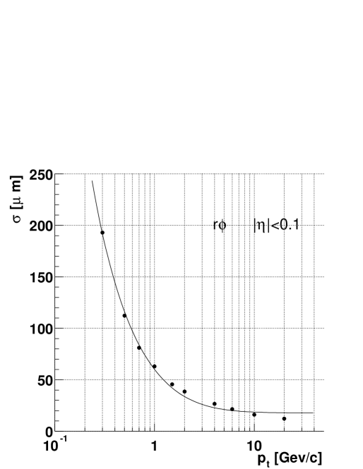
Figure D.1: Impact parameter resolution in $r\phi$ for primary charged pions in the pseudorapidity range $|\eta|<0.1$, fitted to the expression $a\oplus b/p_{\rm t}$.

For the $z$ projection the $p_{\rm t}$-dependence is different and the two contributions cannot be clearly separated. In this case, another important effect has to be considered: the measurement of the $z$ impact parameter is strongly correlated to the measurement of the track polar direction (i.e. of the track dip angle $\lambda=\arctan(p_{z}/p_{\rm t})$). As it can be seen from Table 4.1, in the ITS, the resolution along the $z$ direction is very good in the two central layers (SDD), while it is poorer in the innermost (SPD) and outermost (SSD) layers. This implies that the ITS alone does not provide precise information on the track dip angle. This angle is essentially measured in the TPC, with a resolution that depends on the scatterings the particle has undergone in the ITS. The combination of the error on the polar direction and the errors on the position of the clusters in the ITS determines the resolution on the $z$ projection of the impact parameter.  

Since the multiple scattering contribution to the impact parameter resolution is negligible for high-$p_{\rm t}$ tracks, the values of the resolutions at $p_{\rm t}=20\leavevmode\nobreak\ \mathrm{GeV}/c$, $\simeq 12\leavevmode\nobreak\ \mathrm{\mu m}$ for the $r\phi$ projection and $\simeq 40\leavevmode\nobreak\ \mathrm{\mu m}$ for the $z$ projection, can be estimated from the radial positions and spatial resolutions of the 6 ITS layers. This kind of cross-checks are important in order to understand the results given by the detailed detector simulation and by the track reconstruction algorithm.

Because the number of points is quite large (6), we choose a Monte Carlo approach, rather than an analytical one. High-$p_{\rm t}$ tracks can be approximated to straight lines in the ITS; in fact, for a track of $p_{\rm t}=20\leavevmode\nobreak\ \mathrm{GeV}/c$ in a magnetic field of 0.4 T, the radius of curvature is $R=167\leavevmode\nobreak\ \mathrm{m}$ and the sagitta corresponding to a cord of length $\ell=0.45\leavevmode\nobreak\ \mathrm{m}$ (outer radius of the ITS) is $\ell^{2}/8R\simeq 150\leavevmode\nobreak\ \mathrm{\mu m}$. We, therefore, use the following procedure for the estimation of the impact parameter resolution:

• generate a track as a straight line from the origin $(0,0,0)$ (primary vertex) with a random dip angle $\lambda<45^{\circ}$;

• assign the 6 hits in the ITS layers as the intersection points with 6 cylinders having the radii of the ITS layers (from Table 4.1);

• assign the 6 ‘clusters’ by a gaussian smearing of the positions of the hits in $r\phi$ and in $z$ according to the spatial resolutions of the different detector types (Table 4.1);

• fit a straight line to the 6 ‘clusters’;

• determine the two impact parameter projections as the distances of the fitted line to the origin in the transverse plane and in the $z$ direction;

• iterate the previous steps for $10^{4}$ tracks and estimate the resolutions as the dispersion of the obtained distributions of impact parameters.

Figure D.3 presents the distributions we obtained: the gaussian fits give $\sigma(d_{0}(r\phi))=10\leavevmode\nobreak\ \mathrm{\mu m}$ and $\sigma(d_{0}(z))=70\leavevmode\nobreak\ \mathrm{\mu m}$. While for the $r\phi$ projection the value is very close to that given by the full simulation, for the $z$ projection we get an estimated resolution larger by a factor 2. This difference can be explained by observing that, as already pointed out, the resolution on $d_{0}(z)$ is strongly dependent on the resolution on the track dip angle $\lambda$, which is not so good if only the ITS points are considered. The information from the TPC is essential to determine the polar direction of the track. For high-$p_{\rm t}$ tracks ($>20\leavevmode\nobreak\ \mathrm{GeV}/c$), the overall resolution (TPC–ITS) on $\tan\lambda$ is of about $0.05\%$. If we repeat the same procedure using also this information in the fit, we obtain an estimate of $34\leavevmode\nobreak\ \mathrm{\mu m}$ for the resolution on the $z$ projection of $d_{0}$ (Fig. D.3). Now both estimated resolutions are compatible with the results of the full simulation.  

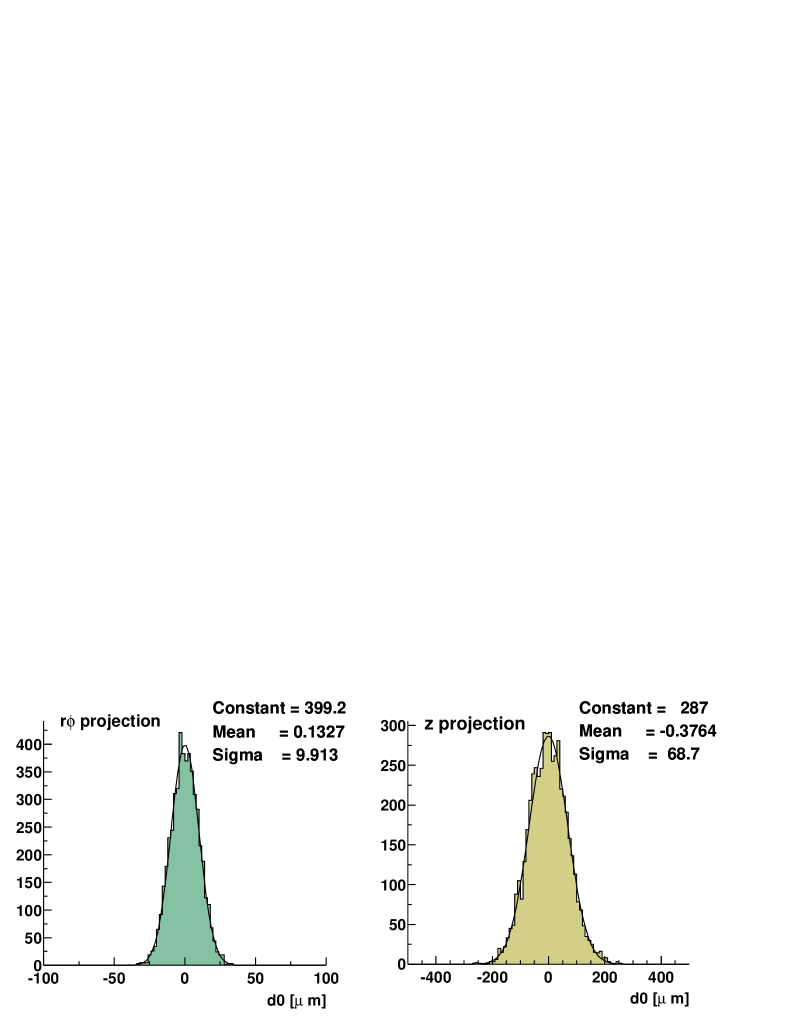
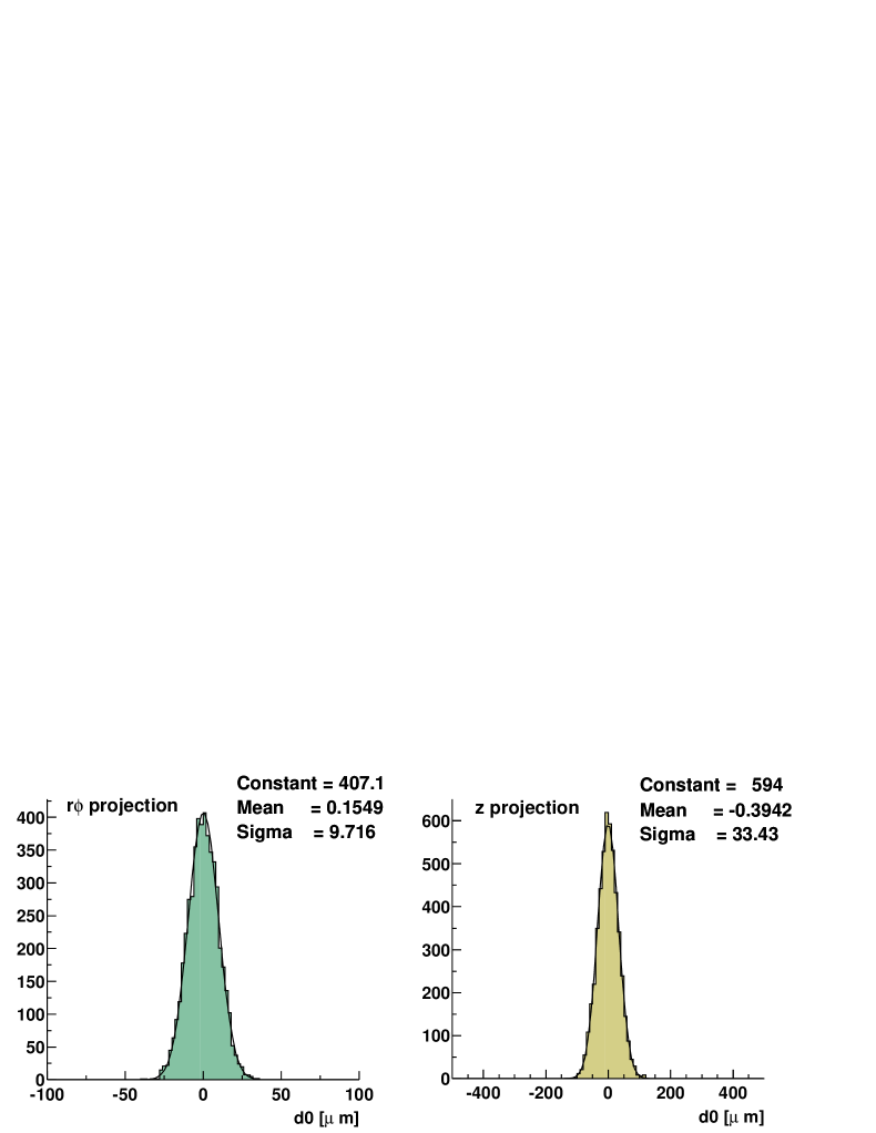
Figure D.2: Impact parameters for high-$p_{\rm t}$ tracks estimated with a Monte Carlo approach based on a simple modeling of the ITS.

Figure D.3: Same as Fig. D.3. In this case the information on track polar direction given by the TPC is included.

As a last point, we study the dependence of the impact parameter resolution on the amount of material in the two pixel layers. In fact, since these detectors are the closest to the interaction point, it is very important to know how much their thickness affects the $d_{0}$ resolution.

All the results presented in this thesis were obtained using in the simulation a total thickness of $400\leavevmode\nobreak\ \mathrm{\mu m}$ of silicon per pixel layer ($200\leavevmode\nobreak\ \mathrm{\mu m}$ for the detector plus $200\leavevmode\nobreak\ \mathrm{\mu m}$ for the readout electronics), which is the current design value. However, only prototypes with a thickness of $600\leavevmode\nobreak\ \mathrm{\mu m}$ have been produced and successfully tested up to now and it is not yet clear if the design parameters can be reached.

In Fig. D.4 we show the effect of thicker pixel layers ($600\leavevmode\nobreak\ \mathrm{\mu m}$) on the resolutions for pions in Pb–Pb: the resolution on the $r\phi$ projection is worse by $\simeq 10\%$ at $p_{\rm t}=1\leavevmode\nobreak\ \mathrm{GeV}/c$.

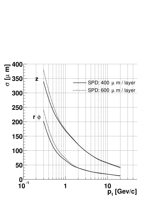
Figure D.4: Impact parameter resolutions for pions in Pb–Pb collisions for two values of the thickness of the Silicon Pixel Detectors: $400\leavevmode\nobreak\ \mathrm{\mu m}$/layer (current design value) and $600\leavevmode\nobreak\ \mathrm{\mu m}$/layer.

References

- [1]
- [2] I.Ya. Pomeranchuk, Dokl. Akad. Nauk. SSSR 78 (1951) 889.
- [3] R. Hagedorn, Nuovo Cimento 35 (1965) 395.
- [4] N. Cabibbo and G. Parisi, Phys. Lett. B59 (1975) 67.
- [5] F. Karsch et al., Phys. Lett. B478 (2000) 447.
-
[6]
U. Heinz, Presentation given for CERN Press Release
‘A New State of Matter’, February 10, 2000:
http://cern.web.cern.ch/CERN/Announcements/2000/NewStateMatter/Slides/ - [7] C. Alcock, The Astrophysics and Cosmology of Quark-Gluon Plasma, in Quark-Gluon Plasma, Springer-Verlag (1990).
- [8] K.G. Wilson, Phys. Rev. D10 (1974) 2445.
- [9] J.D. Bjorken, Phys. Rev. D27 (1983) 140.
- [10] M.C. Abreu et al., NA50 Coll., Phys. Lett. B477 (2000) 28.
- [11] B. Müller and J. Rafelski, Phys. Rev. Lett. 48 (1982) 1066.
- [12] T. Matsui and H. Satz, Phys. Lett. B178 (1986) 416.
- [13] K. Fanebust et al., NA57 Coll., J. Phys. G28 (2002) 1607.
-
[14]
CERN Press Release, February 10, 2000:
http://cern.web.cern.ch/CERN/Announcements/2000/NewStateMatter -
[15]
A short bibliography of the CERN-SPS heavy ion programme:
H. Beker et al., NA44 Coll., Phys. Rev. Lett. 74 (1995) 3340;
I.G. Bearden et al., NA44 Coll., Phys. Rev. Lett. 78 (1997) 2080;
I.G. Bearden et al., NA44 Coll., Phys. Lett. B471 (1999) 6;
G. Agakichiev et al., NA45/CERES Coll., Phys. Lett. B422 (1998) 405;
B. Lenkeit et al., NA45/CERES Coll., Nucl. Phys. A654 (1999) 627c;
B. Lenkeit et al., NA45/CERES Coll., Nucl. Phys. A661 (1999) 23c;
T. Alber et al., NA49 Coll., Phys. Rev. Lett. 75 (1995) 3814;
H. Appelshäuser et al., NA49 Coll., Eur. Phys. J. C2 (1998) 661;
F. Sikler et al., NA49 Coll., Nucl. Phys. A661 (1999) 45c;
M.C. Abreu et al., NA50 Coll., Phys. Lett. B410 (1997) 337;
M.C. Abreu et al., NA50 Coll., Phys. Lett. B450 (1999) 456;
M.C. Abreu et al., NA50 Coll., Phys. Lett. B477 (2000) 28;
R. Klingenberg et al., NA52 Coll., Nucl. Phys. A610 (1996) 306c;
G. Ambrosini et al., NA52 Coll., Phys. Lett. B417 (1998) 202;
G. Ambrosini et al., NA52 Coll., New J. Phys. 1 (1999) 22.1;
E. Andersen et al., WA97/NA57 Coll., Phys. Lett. B449 (1999) 401;
F. Antinori et al., WA97/NA57 Coll., Nucl. Phys. A661 (1999) 130c;
F. Antinori et al., WA97/NA57 Coll., Eur. Phys. J. C14 (2000) 633;
R. Albrecht et al., WA98 Coll., Phys. Rev. Lett. 76 (1996) 3506;
M.M. Aggarwal et al., WA98 Coll., Phys. Rev. Lett. 81 (1998) 4087; 82 (2000) 578;
M.M. Aggarwal et al., WA98 Coll., Phys. Rev. Lett. 83 (1999) 926. - [16] J.D. Bjorken, FERMILAB-PUB-82-59-THY.
- [17] M. Gyulassy and X.N. Wang, Nucl. Phys. B420 (1994) 583, arXiv:nucl-th/9306003.
- [18] R. Baier, Y.L. Dokshitzer, A.H. Mueller, S. Peigné and D. Schiff, Nucl. Phys. B483 (1997) 291, arXiv:hep-ph/9607335.
- [19] J. Jia et al., PHENIX Coll., Nucl. Phys. A715 (2003) 769c.
- [20] C. Adler et al., STAR Coll., arXiv:nucl-ex/0206006.
- [21] S. Mioduszewski et al., PHENIX Coll., arXiv:nucl-ex/0210021.
- [22] S.S. Adler et al., PHENIX Coll., arXiv:nucl-ex/0306021.
- [23] J. Adams et al., STAR Coll., arXiv:nucl-ex/0306024.
- [24] A. Morsch and I. Pshenichnov, ALICE Internal Note, ALICE-INT-2002-34 (2002).
- [25] K.J. Eskola, K. Kajantie, P.V. Ruuskanen and K. Tuominen, Nucl. Phys. A696 (2001) 715.
- [26] K.J. Eskola, K. Kajantie, P.V. Ruuskanen and K. Tuominen, Nucl. Phys. B570 (2000) 379.
- [27] K. Kajantie, Nucl. Phys. A715 (2003) 432c.
- [28] A.D. Martin, R.G. Roberts, W.J. Stirling and R.S. Thorne, Eur. Phys. J C4 (1998) 463.
- [29] H.L. Lai et al., CTEQ Coll., Eur. Phys. J. C12 (2000) 375.
- [30] M. Gluck, E. Reya and A. Vogt, Eur. Phys. J C5 (1998) 461.
-
[31]
V.N. Gribov, L.N. Lipatov, Sov. J. Nucl. Phys. 15
(1972) 438 and 675;
G. Altarelli, G. Parisi, Nucl. Phys. B126 (1977) 298;
Yu.L. Dokshitzer, Sov. Phys. JETP 46 (1977) 641. - [32] K.J. Eskola et al., arXiv:hep-ph/0110348.
- [33] K.J. Eskola, V.J. Kolhinen, C.A. Salgado, Eur. Phys. J. C9 (1999) 61.
- [34] M. Hirai, S. Kumano and M. Miyama, Phys. Rev. D64 (2001) 034003.
- [35] N. Kidonakis, E. Laenen, S. Moch and R. Vogt, arXiv:hep-ph/0105041.
- [36] R. Vogt, Int. J. Mod. Phys. E12 (2003) 211, arXiv:hep-ph/0111271.
- [37] B. Müller and X.N. Wang, Phys. Rev. Lett. 68 (1992) 2437.
- [38] P. Lévai and R. Vogt, Phys. Rev. C56 (1997) 2707.
- [39] M.H. Thoma, Quark-Gluon Plasma 2, ed. R.C. Hwa, p. 51, World Scientific, Singapore (1995).
- [40] M. Gyulassy and M. Plümer, Phys. Lett. B243 (1990) 432.
- [41] R. Baier, Yu.L. Dokshitzer, S. Peigné and D. Schiff, Phys. Lett. B345 (1995) 277.
- [42] R. Baier, Yu.L. Dokshitzer, A.H. Mueller, S. Peigné and D. Schiff, Nucl. Phys. B483 (1997) 291; ibidem B484 (1997) 265.
- [43] B.G. Zakharov, JETP Letters 63 (1996) 952; ibidem 65 (1997) 615.
- [44] R. Baier, Yu.L. Dokshitzer, A.H. Mueller and D. Schiff, Nucl. Phys. B531 (1998) 403.
- [45] B.G. Zakharov, Phys. Atom. Nucl. 61 (1998) 838.
- [46] U.A. Wiedemann and M. Gyulassy, Nucl. Phys. B560 (1999) 345.
- [47] U.A. Wiedemann, Nucl. Phys. B582 (2000) 409; ibidem B588 (2000) 303.
- [48] U.A. Wiedemann, Nucl. Phys. A690 (2001) 731.
- [49] M. Gyulassy, P. Lévai and I. Vitev, Nucl. Phys. B571 (2000) 197; Phys. Rev. Lett. 85 (2000) 5535; Nucl. Phys. B594 (2001) 371.
- [50] R. Baier, Nucl. Phys. A715 (2003) 209c.
-
[51]
C.A. Salgado and U.A. Wiedemann, Phys. Rev. D68 (2003) 014008,
arXiv:hep-ph/0302184;
Numerical routine: http://csalgado.home.cern.ch/csalgado - [52] D.E. Kharzeev, M. Nardi and H. Satz, Phys. Lett. B405 (1997) 14.
- [53] Yu.L. Dokshitzer and D.E. Kharzeev, Phys. Lett. B519 (2001) 199, arXiv:hep-ph/0106202.
- [54] Yu.L. Dokshitzer, V.A. Khoze and S.I. Troyan, J. Phys. G17 (1991) 1602.
- [55] P. Braun-Munzinger et al., Eur. Phys. J. C1 (1998) 123.
- [56] M.C. Abreu et al., NA50 Coll., Eur. Phys. J. C14 (2000) 443.
- [57] T. Sjöstrand, P. Edén, C. Friberg, L. Lönnblad, G. Miu, S. Mrenna and E. Norrbin, Computer Phys. Commun. 135 (2001) 238 (LU TP 00-30, arXiv:hep-ph/0010017).
- [58] K. Adcox et al., PHENIX Coll., Phys. Rev. Lett. 88 (2002) 192303, arXiv:nucl-ex/0202002.
- [59] R. Averbeck et al., PHENIX Coll., Nucl. Phys. A715 (2003) 695c.
- [60] K. Hagiwara et al., Particle Data Group Coll., Phys. Rev. D66 (2002) 010001.
- [61] C. Albajar et al., Phys. Lett. B256 (1991) 121.
-
[62]
F. Abe et al., CDF Coll., Fermilab-Conf-94/134-E;
Fermilab-Conf-94/136-E; Fermilab-Conf-94/141-E;
K. Bazizi, D0 Coll., Fermilab-Conf-94/300-E. - [63] R.V. Gavai et al., arXiv:hep-ph/9411438.
- [64] M. Mangano, P. Nason and G. Ridolfi, Nucl. Phys. B373 (1992) 295.
- [65] M. Bedjidian et al., Hard Probes in Heavy Ion Collisions at the LHC: Heavy Flavor Physics, arXiv:hep-ph/0311048.
- [66] R.J. Glauber and G. Matthiae, Nucl. Phys. B21 (1970) 135.
- [67] C.Y. Wong, Introduction to High-Energy Heavy-Ion Collisions, World Scientific, Singapore (1994).
- [68] B. Hahn, D.G. Ravenhall and R. Hofstadter, Phys. Rev. 101 (1956) 1131.
- [69] V. Emel’yanov, A. Khodinov, S.R. Klein and R. Vogt, arXiv:hep-ph/9909427.
-
[70]
G. Corcella, I.G. Knowles, G. Marchesini,
S. Moretti, K. Odagiri, P. Richardson, M.H. Seymour and B.R. Webber,
JHEP 0101 (2001) 010, arXiv:hep-ph/0011363, arXiv:hep-ph/0201201;
G. Marchesini, B.R. Webber, G. Abbiendi, I.G. Knowles, M.H. Seymour and L. Stanco, Computer Phys. Commun. 67 (1992) 465, Cavendish-HEP-90/26, DESY 91-048. - [71] E. Norrbin and T. Sjöstrand, Eur. Phys. J. C17 (2000) 137.
- [72] D. Abbaneo et al., ALEPH Coll., Eur. Phys. J. C16 (2000) 597-611.
- [73] ALICE Technical Proposal, CERN/LHCC 95-71 (1995).
- [74] Muon Arm, Addendum to the ALICE Technical Proposal, CERN/LHCC 96-32 (1996).
- [75] Transition Radiation Detector, Addendum to the ALICE Technical Proposal, CERN/LHCC 99-13 (1999).
- [76] http://aliweb.cern.ch/offline
-
[77]
ALICE Physics Performance Report, in preparation;
F. Carminati et al., ALICE Internal Note, ALICE-INT-2002-033 (2002). - [78] http://root.cern.ch
- [79] Yellow Report CERN 2000-004.
-
[80]
M. Gyulassy and X.N. Wang, Phys. Rev. D44 (1991) 3501;
M. Gyulassy and X.N. Wang, Comput. Phys. Commun. 83 (1994) 307-331;
The code can be found in http://www-nsdth.lbl.gov/xnwang/hijing/ - [81] http://wwwinfo.cern.ch/asdoc/geantold/GEANTMAIN.html
-
[82]
P. Bilior, Nucl. Instrum. Methods 225 (1984) 352;
M. Regler and R. Frühwirth, Reconstruction of Charged Tracks, in Proc. of the Advanced Study Institute on Techniques and Concepts in High Energy Physics, Plenum Publ. Corp., 1989;
R. Frühwirth, Application of the Filter Methods to the Reconstruction of Tracks and Vertices in Events of Experimental High Energy Physics, HEPHY-PUB 516/88, Vienna (1988);
B. Batyunya, Yu. Belikov, K. afaík, ALICE Internal Note, ALICE-INT-97-24 (1997). - [83] ALICE Time Projection Chamber, Technical Design Report, CERN/LHCC 2000-001.
- [84] Yu. Belikov, private communication.
-
[85]
A. Dainese and N. Carrer, A parameterization of the Kalman filter
track reconstruction in the ALICE TPC, ALICE Internal Note,
ALICE-INT-2003-011 (2003);
the Note can be found at: http://alice.pd.infn.it/Docs.html - [86] A. Badalà, R. Barbera, G. Lo Re, A. Palmeri, G.S. Pappalardo, F. Riggi, ALICE Internal Note ALICE-INT-2001-011 (2001).
- [87] N. Bustreo, B.S. Nilsen, L. Vannucci, ALICE Internal Note ALICE-INT-2001-013 (2001).
-
[88]
A. Dainese and M. Masera, Interaction vertex reconstruction in pp
collisions at LHC with ALICE,
ALICE Internal Note ALICE-INT-2003-027 (2003);
the Note can be found at: http://alice.pd.infn.it/Docs.html - [89] V. Karimäki, CMS Note 1997/051 (1997).
-
[90]
A. Dainese, R. Turrisi and N. Carrer,
Feasibility study for the detection of hadronic decays in
Pb–Pb collisions with ALICE,
ALICE Internal Note ALICE-INT-2002-005 (2002);
the Note can be found at: http://alice.pd.infn.it/Docs.html - [91] ALICE Time Of Flight, Technical Design Report, CERN/LHCC 2000-12.
- [92] P. Saiz et al., Nucl. Instrum. Methods Phys. Res. A502 (2003) 437.
- [93] M. Anguilar-Benitez et al., NA27 Coll., Z. Phys. C41 (1988) 191.
-
[94]
F. James, MINUIT - Function minimization and error analysis,
CERN Program Library Long Writeup D506 (1998),
http://wwwasdoc.web.cern.ch/wwwasdoc/minuit/minmain.html - [95] M. Lunardon and R. Turrisi, Estimation of S/(S+B) ratio for semi-electronic beauty detection in Pb–Pb collisions, ALICE Internal Note, in preparation.
-
[96]
D. Acosta et al., CDF Coll., FERMILAB-PUB/03/217-E,
submitted to Phys. Rev. Lett. July 28, 2003;
C. Chen, Ph.D. thesis, University of Pennsylvania, 2003. - [97] TOTEM, Total cross section, elastic scattering and diffractive dissociation at the LHC: Technical Proposal, CERN-LHCC-99-007; LHCC-P-5 (1999).
- [98] ALICE Physics Performance Report, in preparation, Chapter 6.1.
- [99] B.A. Khiehl, G. Kramer and B. Pötter, Nucl. Phys. B582 (2000) 514, arXiv:hep-ph/0010289.
- [100] C.A. Salgado and U.A. Wiedemann, Phys. Rev. Lett. 89 (2002) 092303.
- [101] Z. Lin and R. Vogt, Nucl. Phys. B544 (1999) 339.
- [102] C.A. Salgado and U.A. Wiedemann, private communication.
- [103] I. Lokhtin, A. Snigrev, Eur. Phys. J. C21 (2001) 155; J. Phys. G27 (2001) 2365.
- [104] ALICE Inner Tracking System, Technical Design Report, CERN/LHCC 99-12.
Acknowledgements
I would like to thank my supervisor, Maurizio Morando, for his constant support and, in particular, for encouraging me to attend schools and conferences and for giving me the possibility to spend long and fruitful periods at CERN during the past three years. There, I was guided by Nicola Carrer and Karel afaík. I am extremely grateful to them for their teachings and their support.
I thank Federico Antinori, Emanuele Quercigh and Rosario Turrisi, for their many useful suggestions that improved my work and this write-up, and all the ALICE group in Padova.
During my stays at CERN I enjoyed many stimulating discussions with
Andreas Morsch, Yura Belikov, Jurgen Schukraft, Jean-Pierre Revol, Guy Paic,
Yiota Foka, Andres Sandoval, Ramona Vogt, Marco Monteno,
Massimo Masera, Fabrizio Pierella, Philippe Crochet, Peter Hristov,
Carlos Salgado, Urs Wiedemann and Nestor Armesto. I wish to thank them all
and I look forward to further collaborate with them.
The love and hard work of my parents allowed me to pursue my studies and researches: thank You.
Many friends accompanied me during these years: Andrea, Andrea, Andrea, Paola, Ilaria, Riccardo, Dario, Patrick, Bernardo, Peter, Toni, Anna, Carlos, Nicola, Rosario, Marco, Alessandro, Lorenzo, Carla, Daniele, Massimo, Francesca.
I want also to thank Café Vieux Carouge for its delicious fondues
and Gino Spagnolo, my landlord, for the wonderful armchair, sitting on which
most of this thesis was written.
All my love goes to a very special person whose charm and sweetness are irreplaceable to me: Barbara.