High-precision measurement of the half-life of ⁶²Ga

Abstract

The $\beta$-decay half-life of ⁶²Ga has been studied with high precision using on-line mass separated samples. The decay of ⁶²Ga which is dominated by a $0^{+}$ to $0^{+}$ transition to the ground state of ⁶²Zn yields a half-life of $T_{1/2}$ = 116.19(4) ms. This result is more precise than any previous measurement by about a factor of four or more. The present value is in agreement with older literature values, but slightly disagrees with a recent measurement. We determine an error weighted average value of all experimental half-lives of 116.18(4) ms.

PPACs: 23.40.-s, 21.10.Tg, 27.50.+e

I Introduction

The Fermi coupling constant $G_{v}$ is most precisely determined from the nuclear $\beta$ decay of nine isotopes ranging from ¹⁰C to ⁵⁴Co [1, 2]. The $0^{+}$ to $0^{+}$ Fermi decays of these isotopes allow to determine a corrected $Ft$ value from the ft values of the individual isotopes and thus the coupling constant $G_{v}$ by means of the relation [1]

$$Ft=ft(1+\delta^{{}^{\prime}}_{R})(1+\delta_{NS}-\delta_{C})=\frac{k}{2G_{v}(1+\Delta_{R}^{v})}.$$ (1)

$f$ is the statistical rate function which strongly depends on the decay Q value for $\beta$ decay and $t$ is the partial half-life of the superallowed $\beta$-decay branch. $\delta^{{}^{\prime}}_{R}$, $\delta_{NS}$ and $\delta_{C}$ are the nucleus dependent part of the radiative correction, the nuclear structure dependent radiative correction, and the isospin-symmetry breaking correction, respectively. $k$ is a constant ($k/(\hbar c)^{6}=(8120.271\pm 0.012)\times 10^{-10}GeV^{-4}s$) and $\Delta_{R}^{v}$ is the transition independent part of the radiative corrections.

The corrected $Ft$ values allow to test the conserved vector current (CVC) hypothesis of the weak interaction. This hypothesis together with the nine most precisely measured $0^{+}\rightarrow 0^{+}$ transitions mentioned above yield an average $Ft$ value of 3072.2(8) s [1].

The coupling constant $G_{v}$ together with the coupling constant for muon decay allows to determine the $V_{ud}$ matrix element of the Cabbibo-Kobayashi-Maskawa (CKM) quark mixing matrix, which in turn can be used to study the unitarity of the CKM matrix. This question has attracted much interest in recent years, as there were indications that the top row of the CKM matrix is not unitary at the 2.2 $\sigma$ level [1, 2]. Recent new measurements [3] seem to indicate that the accepted value of $V_{us}$ might be too low. The new value of $V_{us}$, if confirmed, would restore unitarity of the first row of the CKM matrix (0.9999(16) instead of 0.9968(14) before). A deviation from unitarity would have far reaching consequences for the standard model of the weak interaction and would point to physics beyond the currently accepted model.

Before the existence of physics beyond the standard model can be advocated, the different inputs into the determination of the corrected $Ft$ value which leads to the calculation of the CKM matrix element should be carefully checked. It has turned out that the main uncertainty for the value of the $V_{ud}$ matrix element comes from theoretical uncertainties linked to the different correction factors. The correction which attracted mainly the attention is the isospin-symmetry breaking correction $\delta_{C}$, which is strongly nuclear-model dependent [1, 4, 5]. Model calculations predict this correction to become increasingly important for heavier N=Z, odd-odd nuclei. Measurements with these heavier nuclei should therefore allow to more reliably test this correction.

The aim of the work presented here is to determine with high precision the half-life of ⁶²Ga which is one experimental input to determine the corrected $Ft$ value for this nucleus. This measurement is part of our efforts which include also a measurement of the $\beta$-decay branching ratios for ⁶²Ga and improvements to the Canadian Penning Trap (CPT) mass spectrometer to measure the mass of ⁶²Ga and of its $\beta$-decay daughter ⁶²Zn [6].

The half-life of ⁶²Ga has been measured several times previously. Alburger [7] determined a value of 115.95(30) ms, Chiba et al. [8] obtained a less precise value of 116.4(15) ms, Davids et al. [9] reported a value of 116.34(35) ms, and Hyman et al. [10] recently published a half-life of 115.84(25) ms. These data yield a mean value of 116.00(17) ms. This half-life does not yet reach the required precision of better than $10^{-3}$ in order to include ⁶²Ga in the CVC test and the determination of the CKM matrix element. In the present paper, we report on a measurement which achieves the necessary precision.

II Experimental technique

The experiment was performed at the GSI on-line mass separator. A ⁴⁰Ca beam with an energy of 4.8  A MeV and an average intensity of 50 particle-nA impinged on a niobium degrader foil of thickness 2.7 mg/cm² installed in front of the silicon target of thickness 2.40 mg/cm². The niobium degrader decreased the energy of the primary beam to obtain the highest yield for the ²⁸Si(⁴⁰Ca,$\alpha$pn)⁶²Ga reaction. The beam intensity was controlled in regular time intervals by inserting a Faraday cup upstream of the degrader-target array. A Febiad-E2 source was used to produce a low-energy ⁶²Ga beam which was then mass analysed by the GSI on-line mass separator and delivered to the measuring station. The activity was accumulated on a moving tape device for 350 ms and then moved into the detection setup (transport time about 100 ms). After a delay of 10 ms, the half-life measurement was started. Measurement times of 1600 ms and 1800 ms were used. During the measurement, the beam was deflected well ahead of the collection point. After about 2.2 s, a new cycle started with a new accumulation.

The detection setup consisted of a 4$\pi$ gas detector used to detect $\beta$ particles and a germanium detector for $\gamma$ rays. The $\beta$ detector consists of two single-wire gas counters used in saturation regime and operated with P10 gas slightly above atmospheric pressure. The moving tape transporting the activity passed through a slit between the two detectors. Thin aluminised mylar entrance windows allowed to detect low-energy $\beta$ particles. The detectors were carefully tested before the experiment in order to establish their operation curves and to measure their efficiencies. With a ⁹⁰Sr source we determined an operation plateau between 1450 V and 1900 V and a detection efficiency of about 90%. During the experiment, we used different high voltage values within this plateau. The detector volume was about 5 cm³ for each detector. The counting rate was found to be independent of the gas flow and a gas flow of about 0.15 $l/min$ was used throughout the experiment.

The germanium detector was mounted at a distance of about 4 cm from the source point. It had a photopeak efficiency of 0.8% at 1 MeV. Two $\gamma$-ray spectra were accumulated in a multi-channel analyser in parallel during the run: i) one spectrum which required a $\beta$ coincidence from the gas detector and ii) one spectrum where the germanium detector was running without any coincidence.

The electronics chain for the $\beta$ detector was as follows: The output signal of the two detectors and a pulser signal were fed into one preamplifier (Canberra 2004). The detectors were biased by a Tennelec HV power-supply (TC952A). The preamplifier output was connected to an ORTEC timing-filter amplifier (TFA454) with integration and differentiation times of 100 ns and 20 ns, respectively. The TFA output was fed into a LeCroy octal discriminator (623B). In order to search for systematic effects in our data, we modified the threshold during the experiment as described below. The output of the discriminator was split at the entrance of two LeCroy Dual Gate Generators which defined the non-extendable dead-times of 3 $\mu$s and 5 $\mu$s, respectively. The output signal of the two gate generators were finally passed through a gate generator (GSI GG8000) and a level adapter (GSI LA8010) to adjust the signal length and type for the clock (GSI TD1000) which was started at the beginning of each cycle and which time-stamped each event on a 2 ms/channel basis with 1000 channels. The time stamps were then stored in a memory register (GSI MR2000). During the tape transport, the memory registers were read out, written to tape, and erased for a new cycle.

The clock modules were carefully tested and selected before the experiment. Measurements of their precision and stability have been carried out with respect to a Stanford Research Systems high precision pulse generator (DS345). Tests have been performed at different counting rates (100 kHz to 900 kHz) and with different times per channel (0.5 ms to 20 ms). The modules used had a timing precision of better than 2$\times$10^-6.

The background counting rate was checked before the experiment under experimental conditions. We measured a counting rate of 1.7 counts per second. The average background determined in the half-life fits was about a factor of two higher (see below).

III Half-life measurements

In this section, we will first discuss the results obtained for a reference set of analysis parameters which yields the final half-life value. In the second part, we will test how different analysis parameters may affect the half-life results. In the third part, we will investigate whether the data are subject to any systematic error. For this purpose, we varied different experimental parameters. Finally, the influence of different possible contaminants will be discussed.

A Analysis with reference parameters

The data stored cycle-by-cycle have been analysed off-line with a program package adapted from programs developped at Chalk River [11]. This package includes a program to select cycles according to user defined criteria. The selection criteria are the number of counts in the spectrum for a given cycle and the $\chi^{2}$ value of a least-square fit of a user defined function (see below) to the data. For a typical high-statistics run (e.g. run 10), about 10% of the original data has been rejected due to low statistics, whereas less than 1% of the data did not satisfy our fit quality criterium, i.e. either the fit did not converge after 500 iterations or we obtained a too poor $\chi^{2}$ value. Therefore, if one excludes low-statistics cycles, at maximum 1% of the cycles were rejected. We do not expect that such a low rejection rate will bias our final result.

The fitting procedure is taken from a text book [12]. The first condition rejects cycles where e.g. the primary beam was off or where other technical problems reduced the counting rate significantly. The second condition reject cycles with gas-detector sparks. The reference conditions for this selection are a cutoff limit of 20 counts per cycle and a reduced $\chi^{2}$ value of 2 for the cycle fits. The fit was performed by assuming a one-component exponential and a long-lived fixed background, the latter being determined by an iterative procedure separately for each run. Variations of these parameters are discussed below.

For selected cycles, the program generates a simulated data set for which all characteristics but the half-life are determined by the experimental cycle. These simulated data are then subjected to a pre-defined dead-time and stored cycle-by-cycle on disk. We used a half-life of 116.40 ms in the simulations.

FIG. 1.: (Color online) (a) Experimental decay spectrum for run 29. The spectrum has been corrected for dead-time. The half-life determined for this run is 116.22(16) ms. (b) Simulated spectrum generated with the same characteristics as the experimental spectrum, but an input half-life of 116.40 ms. After dead-time correction, the half-life determined is 116.55(16) ms.

The second step in the analysis procedure is a correction cycle-by-cycle of the dead-time. This is achieved by a correction of each channel with a factor of $f_{dt}=1/(1+t_{dt}R)$, where $t_{dt}$ is the non-extendable dead-time per event (3$\mu$s or 5$\mu$s) and $R$ is the counting rate (1/s) determined from the channel content. After dead-time correction, all selected cycles are summed to yield the decay-time spectrum of a given run. 39 different runs with run times as long as 4 h at maximum and varying experimental conditions (high voltage of the gas detector, CFD threshold, cycle time, transport tape) were accumulated. In total, about 38$\times$10^{6 62}Ga decays have been detected.

In figure 1a, we show the experimental spectrum of one run corrected for dead-time. The fit of this particular run which lasted about 4h yielded a half-life of 116.22(16) ms. Part b of the figure shows the simulated spectrum. Here a half-life of 116.55(16) ms resulted.

Similar results were obtained for the other runs. Figure 2a shows the half-life determined for each of the 39 runs for the data set with a dead-time of 5 $\mu$s. The fits of the individual runs were performed with a decay component for ⁶²Ga and a constant background. The error-weighted average of the half-life is 116.18(3) ms. These data have been analysed with the reference conditions defined above. The reduced $\chi^{2}$ value of the averaging fit is 1.60.

Figure 2b shows the reduced $\chi^{2}$ value of the fits of the individual runs. In general, the values are below 1.1. Two runs are at a reduced $\chi^{2}$ value of about 1.13 and two more above 1.2. These high $\chi^{2}$ values indicate a rather low probability (below 0.1%) for the fitted distribution being the true distribution. We analysed these runs very carefully by e.g. cutting them in up to four ”sub-runs” to see whether there is any indication of increased detector sparking or any other experimental problem. As we did not find any difference between these runs and those with lower $\chi^{2}$ values, we assume that these high values are a result of the tails of the probability distribution of $\chi^{2}$. Removal of these runs would not have changed the final result by any means.

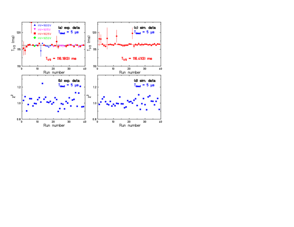
FIG. 2.: (Color online) (a) Experimental half-lives as determined for the different runs. The results shown originate from the data set with a preset dead-time of 5$\mu$s. The average results in a half-life value of 116.18(3) ms. The reduced $\chi^{2}$ value for the averaging procedure is 1.6. (b) Reduced $\chi^{2}$ values for the fits of the experimental spectra of the individual runs. (c) and (d) show the same information as (a) and (b), however, for the simulated decay distributions. Here a half-life of 116.41(3) ms is obtained, in agreement with the input half-life of 116.40 ms. The averaging procedure yields here a reduced $\chi^{2}$ of better than unity.

In figures 2c,d, we plot the same information for the simulated data. The average value for the half-life is 116.41(3) ms in agreement with the input value of 116.40 ms. Most of the reduced $\chi^{2}$ values are close to unity, but there are again runs with higher values from the tails of the $\chi^{2}$ probability distribution. The fact that the half-life result for the simulated data corresponds to the input half-life shows that the dead-time correction is done correctly. An omission of the dead-time correction for the 5$\mu$s data would yield a half-life that is longer by about 0.15 ms.

The data with a fixed dead-time of 3$\mu$s were analysed in a similar way, including again a comparison with simulations. The results are in perfect agreement with the 5$\mu$s data set. In figure 3, we show the half-life values for the individual runs as deduced from this data set. The average value is 116.18(3) ms. The reduced $\chi^{2}$ distribution is very similar to the one of the first data set. The fact that we obtain the same results for the two data sets with different dead-time values indicates again that the dead-time correction in the data analysis is handled properly.

Another way to track down possible problems with the dead-time correction is to fit the experimental and simulated data for different parts of the spectra. This uses the fact that the data at the beginning of the cycle are, due to the higher counting rate, more strongly influenced by the dead-time than the data later in the cycle. In figure 4, we present this analysis of the data for the two data sets, experiment and simulations. The half-life shows indeed very little variation as a function of the starting point of the fit and the half-lives obtained vary around the value obtained when the whole spectrum is fitted.

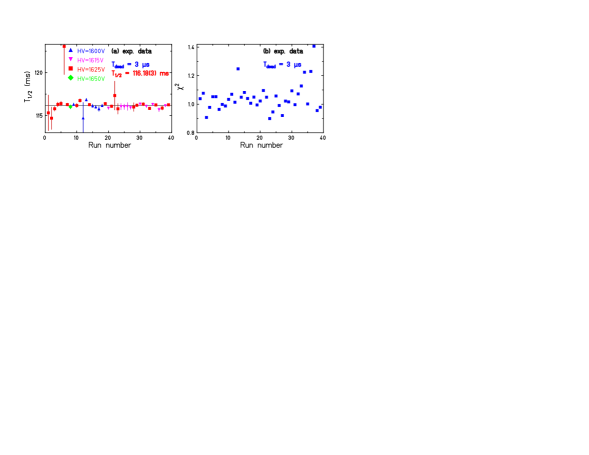
FIG. 3.: (Color online) (a) Experimental half-lives as determined from the data set registered with a fixed dead-time of 3 $\mu$s. The error weigthed average value is 116.18(3) ms with a reduced $\chi^{2}$ of 1.65. (b) Reduced $\chi^{2}$ values for the fits of the different runs.

B Influence of analysis parameters

The selection of cycles can be performed with different parameter values. This selection may influence the final result considerably. We therefore tested the different selection criteria extensively.

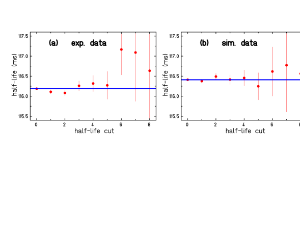
FIG. 4.: (Color online) (a) Experimental half-lives as determined for cuts in the time distribution. The data point shown at an x value of zero is the half-life obtained when the whole spectrum is fitted. The data point at an x value of 1 originates from a fit where the first 116 ms, i.e. the first half-life of ⁶²Ga, of the spectrum were omitted etc. The solid line corresponds to the half-life value without cut. (b) Same cuts performed on the simulated data. The data used for this analysis include all runs with a 5$\mu$s dead-time.

The most important selection parameter is the $\chi^{2}$ value of the fit of the individual cycles. We performed tests with reduced $\chi^{2}$ limits of 1.5, 2, 5, 20, 2000, and 20000. The reduced $\chi^{2}$ value of the cycle fits has to be equal to or smaller than the chosen $\chi^{2}$ value to be taken into account for further analysis. No significant change of the half-life obtained was observed for values of 2 and higher. However, a too tight limit on $\chi^{2}$ yields longer half-lives. A reduced $\chi^{2}$ limit of 1.5 in the cycle selection yields a half-life about 0.2% longer than for higher values.

The use of a reduced $\chi^{2}$ value higher than two does not alter the resulting final half-life, however, the $\chi^{2}$ value of the individual runs increases significantly with increasing $\chi^{2}$ limit, as less and less detector sparks are eliminated. We finally chose a reduced $\chi^{2}$ value of 2 to efficiently remove cycles with detector sparks.

An additional selection parameter is the number of counts for a cycle. We varied this parameter but could not find any systematic behaviour as a function of its value. The final analysis was performed with a value of 20. This removes basically all cycles with low activity.

As mentioned above, the cycle selection was performed by fitting with only one decay component and a fixed constant background. The fixed constant background option was chosen to avoid negative background fit values that may occur due to the very low statistics per cycle. The fixed background was determined iteratively for each run individually. This procedure converged after only two or three iterations. We performed also analyses with background values different from those determined by the iterative procedure. It turned out that slightly different half-lives were obtained only when reduced $\chi^{2}$ values smaller than two were used.

To test the fitting procedure, we performed also fits of our data with the MINUIT [13] fit package. These fits performed for individual runs as well as for a sum spectrum of all runs yield, after dead-time correction, precisely the same results as the least-square procedure from a text book [12] used in the main analysis.

C Search for systematic effects due to experimental conditions

During the experiment, certain experimental parameters were changed to study their influence on the half-life determined. For this purpose, we used two different values for the CFD threshold which triggered the decay events. Runs up to run number 17 were performed with a threshold value of -0.3 V. For the 5$\mu$s data, these runs give an average half-life of 116.26(6) ms. The runs from number 18 on used a slightly different value of -0.35 V. Here the average half-life is 116.14(4) ms. For the 3$\mu$s data, similar values were obtained. These values agree with each other at the 1.4 $\sigma$ level.

Another parameter changed periodically during the data taking is the detector high-voltage. The values used varied between 1600 V and 1650 V. In figure 2a,b, the runs with different high-voltage values are shown by different symbols. No systematic effect was observed. The average half-lives determined are 116.28(7) ms, 116.10(6) ms, 116.21(5) ms, and 116.00(24) ms for the high-voltage values of 1600 V, 1615 V, 1625 V, and 1650 V, respectively. The results for the 3$\mu$s data set is in agreement with the 5$\mu$s data.

Runs 1-14 were performed with a decay time of 1600 ms, whereas a decay time of 1800 ms was used for the rest of the runs. This change did not induce any observable systematic effect. Finally the transport tape was changed after run 14 to ensure that long-lived activities do not alter the results. No effect was observed.

Within the tests performed our data are not subject to any experimental bias. We therefore do not correct our data for systematic errors due to experimental parameters.

D Search for contaminants

Contaminants which are produced in the same reaction and transported in the same way as ⁶²Ga may alter the observed half-life significantly. In general, their half-life is different from the half-life of ⁶²Ga and their influence has to be studied carefully.

In an isobaric chain separated by a mass separator, the half-lives change significantly from one isotope to the other. As the less exotic isotopes have normally longer half-lives and are usually produced with much higher cross sections, an isobaric contamination not corrected for properly yields longer half-lives.

Our data are possibly subject to different kinds of contamination:

• As the mass separation is not perfect, isotopes with masses A=61 or A=63 might contaminate our data. However, at the GSI on-line separator neighboring masses are suppressed by a factor of the order of $10^{4}$ which does not take differences in production cross-section and half-life into account. This high selectivity is confirmed by the fact that no $\gamma$ rays from mass 61 or 63 isotopes were observed in the $\beta$-particle gated $\gamma$ spectra which yields a suppression factor well above 10⁴.

• ⁶²Zn ($T_{1/2}$=9.2h) is produced i) directly in the ion source of the mass separator and transported to the collection point and ii) by the decay of ⁶²Ga. However, due to its low $Q_{EC}$ value of 1627 keV, ⁶²Zn decays mainly by electron capture. As the half-life of ⁶²Ga was determined by measuring the time characteristics of $\beta$ particles, ⁶²Zn is not expected to alter the half-life value of ⁶²Ga. In addition, its half-life is very long compared to that of ⁶²Ga so that its contribution is in the worst case expected to yield a constant background. These findings are confirmed by the absense of $\gamma$ rays from the decay of ⁶²Zn in the $\beta$-gated $\gamma$ spectrum.

• ⁶²Cu ($T_{1/2}$=9.7 min) is certainly the most important contaminant because its half-life is short enough to be a concern. It is either produced directly in the ion source of the mass separator and implanted as a mass-separated beam or produced in the decay of the ⁶²Zn activity collected on the tape. The latter contribution can safely be discarded, as it is governed by the ⁶²Zn half-life which is very long.

  To determine the influence of ⁶²Cu produced in the mass separator source and collected together with ⁶²Ga, we attempted to fit the time distributions for the individual runs as well as for the sum of all runs by adding a second exponential with the time constant of ⁶²Cu to the fit function. However, the fit reduces this contribution to a value in agreement with zero. If we impose a ⁶²Cu contribution by fixing the amount of ⁶²Cu, the fit reduces the background, but keeps the ⁶²Ga half-life constant. In fact the half-life changes by 0.01 ms, if we compare a fit without any ⁶²Cu contribution and a fit with the highest possible contribution of ⁶²Cu which is defined by the fact that no constant background is left over in the fit. As the constant background cannot become negative, the ⁶²Ga half-life becomes shorter if the ⁶²Cu contribution is still increased. In the same way, the reduced $\chi^{2}$ value of the fit stays unity until the background is zero and the ⁶²Ga half-life becomes shorter. This finding means that a possible ⁶²Cu contribution is comparable to a constant background and we can not distinguish both, i.e. a possible ⁶²Cu contamination does not alter the ⁶²Ga half-life. These results are shown graphically in figure 5.

  

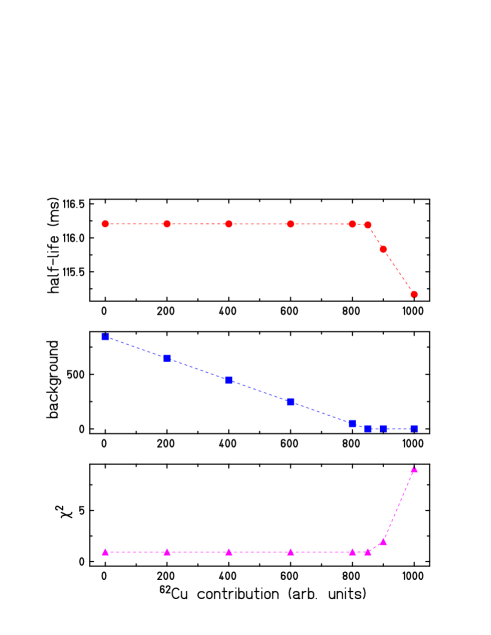
  FIG. 5.: (Color online) Part (a) shows the variation of the ⁶²Ga half-life as a function of the amount of contamination by ⁶²Cu imposed in the fit. Part (b) indicates how the constant background decreases as the ⁶²Cu contribution increases, whereas part (c) demonstrates that the fit quality is not altered as long as the constant background can be reduced by the fit. The reduced $\chi^{2}$ value and the half-life of ⁶²Ga change only, once the constant background has vanished and the ⁶²Cu contribution is still increased. The whole data set with a dead-time of 5$\mu$s is used for this analysis.

  We searched also for a ⁶²Cu contamination in the $\beta$-gated $\gamma$ spectrum. However, none of the known $\gamma$ rays of ⁶²Cu could be identified which supports the conclusion that ⁶²Cu does not play an important role in the present experiment.

• ⁶²Ge ($T_{1/2}$=129$\pm$35 ms [14]) can also be produced by the ²⁸Si(⁴⁰Ca,$\alpha$2n) reaction used in the present experiment. The production of this more exotic nucleus, however, is expected to be significantly smaller. Although fusion-evaporation codes do not very reliably predict very small cross sections, it is worth mentioning that the HIVAP code [15] predicts ⁶²Ge with yields which are a factor of $10^{-5}$ smaller than those for ⁶²Ga. In addition, the release efficiency of the Febiad-E2 ion source for germanium isotopes is known to be much smaller than that for gallium isotopes which reduces the probability of an important ⁶²Ge contamination even more. As the half-life of ⁶²Ge is rather close to the one of ⁶²Ga, large amounts of ⁶²Ge would be necessary to alter the half-life determined for ⁶²Ga. We therefore conclude that the influence of ⁶²Ge is negligible.

E Final experimental result

The evaluation of possible systematic errors from contaminants or other sources shows that no such corrections to the half-life are necessary. Therefore, our experimental result with its statistical error is 116.18(3) ms. However, when averaging the different runs we obtain a reduced $\chi^{2}$ value of 1.6 which indicates that there might be some hidden inconsistencies between the different runs. A possible explanation could be that our cycle selection procedure does not remove all detector sparks. The probability that the fit function (a constant in our case) is the correct function to describe the data is only 1% with a reduced $\chi^{2}$ value of 1.6 [12].

We therefore apply a procedure proposed by the Particle Data Group [16] and multiply the error bars of the individual runs by the square-root of the reduced $\chi^{2}$ value obtained from the averaging procedure. The subsequent averaging gives the final experimental value of 116.19(4) ms.

IV Discussion

Our experimental result of 116.19(4) ms has to be compared with other half-life measurements from the literature. In table I, we list all published half-life measurements for ⁶²Ga. Our result is in excellent agreement with all measurements, but the most recent publication by Hyman et al. [10]. In fact, the discrepancy of the present result with the one of Hyman et al. is at the 1.2 $\sigma$ level. When averaging all experimental values, we obtain an error weighted average value of 116.18(4) ms with a reduced $\chi^{2}$ value of 0.68.

Three measurements for the $\beta$-decay branching ratio of ⁶²Ga have been published recently [10, 17, 18]. All measurements yield consistent results of 0.120(21)%, 0.12(3)%, and 0.106(17)% for the population and decay of the first excited state in ⁶²Zn. Hyman et al.[10] used these results and shell-model calculations to determine the superallowed branching ratio to be 99.85${}^{+0.05}_{-0.15}$%. By using this result together with the measured Q value [9] of 9171(26) keV and the half-life of 116.18(4) ms, we obtain an $ft$ value of $ft$ =(3056$\pm$47)s for ⁶²Ga. When taking into account the correction factors as calculated by Towner and Hardy [1], we finally get a corrected $Ft$ value of $Ft$ = (3056$\pm$47)s (the $Ft$ value numerically does not change compared to the $ft$ value, because the correction factors $\delta^{{}^{\prime}}_{R}$ and $\delta_{c}-\delta_{NS}$ are similar in size). This value is in agreement with the average value from the nine precisely measured transitions between ¹⁰C and ⁵⁴Co of $Ft$ =3072.2(8) s [1].

The large uncertainty of our corrected $Ft$ value comes almost entirely from the error associated with the poorly known $\beta$-decay Q value. The correction factors can therefore not yet be tested with the experimental precision reached up to now. A much more precise value for the Q value is needed for this purpose. However, assuming that CVC holds and the correction factors are correct, we can determine the Q value for the decay of ⁶²Ga. We obtain a value of 9180(4) keV which is consistent with the value determined by Hyman et al. [10] of 9183(6) keV.

V Conclusions

We have performed a high-precision measurement of the half-life of ⁶²Ga. The half-life was determined by detecting the $\beta$ particles from a ⁶²Ga source produced at the GSI on-line mass separator. The result of T_1/2 = 116.19(4) ms obtained in this work is in agreement with older half-life values from the literature. The present result is more than a factor of four more precise than any previous result. We determine an error-weighted mean value of 116.18(4) ms for the half-life of ⁶²Ga.

This half-life value is now precise enough to contribute to a stringent test of CVC above Z=27 as soon as a more precise $\beta$-decay Q value and a refined value of the $\beta$-decay branching ratios are known. ⁶²Ga can then also be used to test the correction factors calculated to determine the nucleus independent $Ft$ value. Work on these issues is under way.

REFERENCES

- [1] I. S. Towner and J. C. Hardy, Phys. Rev. C 66, 035501 (2002).
- [2] J. C. Hardy et al., Nucl. Phys. A509, 429 (1990).
- [3] A. Sher et al., arXiv:hep-ex/0305042 (2003).
- [4] W. E. Ormand and B. A. Brown, Phys. Rev. C 52, 2455 (1995).
- [5] H. Sagawa, N. V. Giai, and T. Suzuki, Phys. Rev. C 53, 2163 (1996).
- [6] G. Savard, priv. communication.
- [7] D. E. Alburger, Phys. Rev. C 18, 1875 (1978).
- [8] R. Chiba et al., Phys. Rev. C 17, 2219 (1978).
- [9] C. N. Davids, C. A. Gagliardi, M. J. Murphy, and E. B. Norman, Phys. Rev. C 19, 1463 (1979).
- [10] B. C. Hyman et al., Phys. Rev. C 68, 015501 (2003).
- [11] V. T. Koslowsky et al., Nucl. Instrum. Meth. Phys. Res. A401, 289 (1997).
- [12] P. R. Bevington and D. K. Robinson, McGraw Hill Higher Education 3rd edition, p. 142ff (2003).
- [13] http://wwwasdoc.web.cern.ch/wwwasdoc/minuit/minmain.html, CERN program library .
- [14] M. J. López Jiménez et al., Phys. Rev. C 66, 025803 (2002).
- [15] W. Reisdorf, Z. Phys. A 300, 227 (1981).
- [16] K. Hagiwara et al., Phys. Rev. D 66, 010001 (2002).
- [17] B. Blank, Eur. Phys. J. A15, 121 (2002).
- [18] J. Döring et al., Proc. ENAM2001 Springer Verlag, 323 (2002).