How well do we know the electromagnetic form factors of the proton?

Abstract

Several experiments have extracted proton electromagnetic form factors from elastic cross section measurements using the Rosenbluth technique. Global analyses of these measurements indicate approximate scaling of the electric and magnetic form factors ($\mu_{p}G_{E_{p}}/G_{M_{p}}\approx 1$), in contrast to recent polarization transfer measurements from Jefferson Lab. We present here a global reanalysis of the cross section data aimed at understanding the disagreement between the Rosenbluth extraction and the polarization transfer data. We find that the individual cross section measurements are self-consistent, and that the new global analysis yields results that are still inconsistent with polarization measurements. This discrepancy indicates a fundamental problem in one of the two techniques, or a significant error in polarization transfer or cross section measurements. An error in the polarization data would imply a large error in the extracted electric form factor, while an error in the cross sections implies an uncertainty in the extracted form factors, even if the form factor ratio is measured exactly.

I INTRODUCTION

The electromagnetic structure of the proton is described by the electric and magnetic form factors. Over the past several decades, a large number of experiments have measured elastic electron-proton scattering cross sections in order to extract the electric and magnetic form factors, $G_{E_{p}}(Q^{2})$ and $G_{M_{p}}(Q^{2})$ (where $-Q^{2}$ is the four-momentum transfer squared), using the Rosenbluth technique Rosenbluth (1950). The electric and magnetic form factors have been extracted up to $Q^{2}\approx 7$ GeV² by direct Rosenbluth separations, and these measurements indicate approximate form factor scaling, i.e., $\mu_{p}G_{E_{p}}/G_{M_{p}}\approx 1$ (where $\mu_{p}$ is the magnetic dipole moment of the proton), though with large uncertainties in $G_{E_{p}}$ at the highest $Q^{2}$ values Walker et al. (1994); Walker (1989).

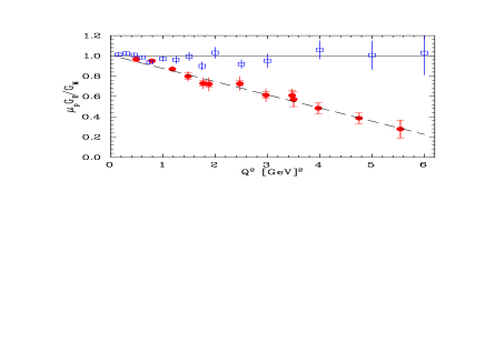
Figure 1: Ratio of electric to magnetic form factor as extracted by Rosenbluth measurements (hollow squares) and from the JLab measurements of recoil polarization (solid circles). The dashed line is the fit to the polarization transfer data.

More recently, elastic electron-proton polarization transfer measurements have been performed to obtain the ratio $G_{E_{p}}/G_{M_{p}}$. A low $Q^{2}$ measurement at MIT-Bates Milbrath et al. (1999, 1998) obtained values of $G_{E_{p}}/G_{M_{p}}$ consistent with previous Rosenbluth separations. Later experiments at Jefferson Lab (JLab) extended these measurements up to $Q^{2}=5.6$ GeV² Jones et al. (2000); Gayou et al. (2001, 2002), and show significant deviations from form factor scaling. They show a roughly linear decrease of the value of $\mu_{p}G_{E_{p}}/G_{M_{p}}$ from unity at low $Q^{2}$ to approximately 0.3 at $Q^{2}=5.6$ GeV². Figure 1 shows the JLab polarization transfer measurements from refs. Jones et al. (2000); Gayou et al. (2002), along with a global Rosenbluth analysis of the cross section measurements Walker et al. (1994). While the polarization transfer technique allows much better measurements at high $Q^{2}$ values, there is a significant discrepancy even in the region where both techniques have comparable uncertainties.

When we combine the cross sections with polarization transfer measurements to extract the form factors (see Sect. III.6, or Ref. Brash et al. (2002)), we find that the values obtained for $G_{E_{p}}$ are significantly different, while $G_{M_{p}}$ differs only at the few percent level, compared to extractions that use only the cross sections. Clearly, it is necessary to understand the discrepancy in the extracted ratio before we can be confident in our knowledge of $G_{E_{p}}$ and, to a lesser extent, $G_{M_{p}}$. The Rosenbluth data is more sensitive to systematic uncertainties, and it has been suggested that the different Rosenbluth extractions are inconsistent, and thus unreliable. We will examine the consistency of the Rosenbluth measurements to test this suggestion. However, even if it is demonstrated that the cross sections going into the Rosenbluth extractions were incorrect, it would not completely solve the problem. The polarization measurements determine only the ratio of $G_{E_{p}}$ to $G_{M_{p}}$, and so reliable cross sections are still needed to extract the actual values of the form factors. Finally, if the discrepancy arises from a fundamental problem with either of these techniques, it may have implications for other measurements.

The goal of this analysis it to better understand the discrepancy between the Rosenbluth and polarization transfer results. We begin by demonstrating that the individual Rosenbluth measurements yield consistent results when analyzed independently, so that the normalization uncertainties between different measurements do not impact the result. We then perform a global analysis of the cross section measurements, and determine that the results cannot be made to agree with the polarization results by excluding an small set of measurements, or by making reasonable modifications to the relative normalization of the various experiments. The paper is organized as follows: In section II, we will review the two techniques and summarize the current measurements of the form factors. In section III, we present a new Rosenbluth analysis of the cross section measurements, and compare this to the polarization transfer results and examine possible scenarios that might explain the discrepancy between the techniques, such as problems with individual data sets or improper treatment of normalization uncertainties when combining cross sections from different experiments. In section IV we will discuss the results of the analysis and implications of the discrepancy between the two techniques. Finally, in section V, we summarize the results and discuss further tests that can be performed to help explain the disagreement between the techniques.

II OVERVIEW OF FORM FACTOR MEASUREMENTS

We begin with a brief description of the Rosenbluth separation and recoil polarization techniques, focusing on the existing data and potential problems with the extraction techniques.

II.1 Rosenbluth Technique

The unpolarized differential cross section for elastic scattering can be written in terms of the cross section for scattering from a point charge and the electric and magnetic form factors:

$$\frac{d\sigma}{d\Omega}=\sigma_{\rm Mott}\biggl{[}\frac{G_{E_{p}}^{2}+\tau G_{M_{p}}^{2}}{1+\tau}+2\tau G_{M_{p}}^{2}\tan^{2}{(\theta_{e}/2)}\biggr{]},$$ (1)

where $\theta_{e}$ is the electron scattering angle, and $\tau=Q^{2}/4M_{p}^{2}$. One can then define a reduced cross section,

$$\sigma_{R}\equiv\frac{d\sigma}{d\Omega}\frac{\epsilon(1+\tau)}{\sigma_{\rm Mott}}=\tau G_{M_{p}}^{2}(Q^{2})+\epsilon G_{E_{p}}^{2}(Q^{2}),$$ (2)

where $\epsilon$ is the longitudinal polarization of the virtual photon ($\epsilon^{-1}=1+2(1+\tau)\tan^{2}{(\theta_{e}/2)}$). At fixed $Q^{2}$, i.e., fixed $\tau$, the form factors are constant and $\sigma_{R}$ depends only on $\epsilon$. A Rosenbluth, or longitudinal-transverse (L-T), separation involves measuring cross sections at several different beam energies while varying the scattering angle to keep $Q^{2}$ fixed while varying $\epsilon$. $G_{E_{p}}^{2}$ can then be extracted from the slope of the reduced cross section versus $\epsilon$, and $\tau G_{M_{p}}^{2}$ from the intercept. Note that because the $G_{M_{p}}^{2}$ term has a weighting of $\tau/\epsilon$ with respect to the $G_{E_{p}}^{2}$ term, the relative contribution of the electric form factor is suppressed at high $Q^{2}$, even for $\epsilon=1$.

Because the electric form is extracted from the difference of reduced cross section measurements at various $\epsilon$ values, the uncertainty in the extracted value of $G_{E_{p}}^{2}(Q^{2})$ is roughly the uncertainty in that difference, magnified by factors of $(\Delta\epsilon)^{-1}$ and $(\tau G_{M_{p}}^{2}/G_{E_{p}}^{2})$. This enhancement of the experimental uncertainties can become quite large when the range of $\epsilon$ values covered is small or when $\tau$ ($=Q^{2}/4M_{p}^{2}$) is large. This is especially important when one combines high-$\epsilon$ data from one experiment with low-$\epsilon$ data from another to extract the $\epsilon$-dependence of the cross section. In this case, an error in the normalization between the data sets will lead to an error in $G_{E_{p}}^{2}$ for all $Q^{2}$ values where the data are combined. If $\mu_{p}G_{E_{p}}=G_{M_{p}}$, $G_{E_{p}}$ contributes at most 8.3% (4.3%) to the total cross section at $Q^{2}=5(10)$ GeV², so a normalization difference of 1% between a high-$\epsilon$ and low-$\epsilon$ measurement would change the ratio $\mu_{p}G_{E_{p}}/G_{M_{p}}$ by 12% at $Q^{2}=5$ GeV² and 23% at $Q^{2}=10$ GeV², more if $\Delta\epsilon<1$. Therefore, it is vital that one properly account for the uncertainty in the relative normalization of the data sets when extracting the form factor ratios. The decreasing sensitivity to $G_{E_{p}}$ at large $Q^{2}$ values limits the range of applicability of Rosenbluth extractions; this was the original motivation for the polarization transfer measurements, whose sensitivity does not decrease as rapidly with $Q^{2}$.

II.2 Recoil Polarization Technique

In polarized elastic electron-proton scattering, $p(\vec{e},e^{\prime}\vec{p})$, the longitudinal ($P_{l}$) and transverse ($P_{t}$) components of the recoil polarization are sensitive to different combinations of the electric and magnetic elastic form factors. The ratio of the form factors, $G_{E_{p}}/G_{M_{p}}$, can be directly related to the components of the recoil polarization Dombey (1969); Akheizer and Rekalo (1974); Arnold et al. (1981); Perdrisat et al. (1993):

$$\frac{G_{E_{p}}}{G_{M_{p}}}=-\frac{P_{t}}{P_{l}}\frac{(E_{e}+E_{e^{\prime}})\tan{(\theta_{e}/2)}}{2M_{p}},$$ (3)

where $E_{e}$ and $E_{e}^{\prime}$ are the incoming and scattered electron energies, and $P_{l}$ and $P_{t}$ are the longitudinal and transverse components of the final proton polarization. Because $G_{E_{p}}/G_{M_{p}}$ is proportional to the ratio of polarization components, the measurement does not require an accurate knowledge of the beam polarization or analyzing power of the recoil polarimeter. Estimates of radiative corrections indicate that the effects on the recoil polarizations are small and at least partially cancel in the ratio of the two polarization component Afanasev (2001).

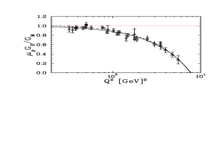
Figure 2: Ratio of electric to magnetic form factor as extracted by recoil polarization measurements at MIT-Bates (solid squares) and JLab (hollow symbols). The solid line is the fit to Jones et al. (2000); Gayou et al. (2002) (diamonds and triangles) from Ref. Gayou et al. (2002), while the dashed line is a combined fit, including the systematic uncertainties (assumed to be fully correlated within each data set).

Figure 2 shows the measured values of $\mu_{p}G_{E_{p}}/G_{M_{p}}$ from the MIT-Bates Milbrath et al. (1999, 1998) and JLab Jones et al. (2000); Gayou et al. (2001, 2002) experiments, both coincidence and single arm measurements, along with the linear fit of Ref. Gayou et al. (2002) to the data from Jones et al. (2000); Gayou et al. (2002):

$$\mu_{p}G_{E_{p}}/G_{M_{p}}=1-0.13(Q^{2}-0.04),$$ (4)

with $Q^{2}$ in GeV². Comparing the data to the fit, the total $\chi^{2}$ is is 34.9 for 28 points, including statistical errors only. Assuming that the systematic uncertainties for each experiment are fully correlated, we can vary the systematic offset for each data set and the total $\chi^{2}$ decreases to 33.6. If we allow the systematic offset to vary for each data set and refit the $Q^{2}$-dependence to all four data sets using the same two-parameter fit as above, i.e.,

$$\mu_{p}G_{E_{p}}/G_{M_{p}}=1-\alpha(Q^{2}-Q_{0}^{2}),$$ (5)

for $Q^{2}>Q_{0}^{2}$, unity for $Q^{2}<Q_{0}^{2}$. We obtain $\alpha=0.135\pm 0.008$, $Q_{0}^{2}=0.24\pm 0.08$, and $\chi^{2}$=28.1 for 26 degrees of freedom (dashed line in Fig. 2). The systematic offsets are small (consistent with zero) for all of the data sets except the low $Q^{2}$ JLab measurement Jones et al. (2000), which is increased by nearly the full (correlated) systematic uncertainty. This fit not only has a better $\chi^{2}$, but also decreases the deviation from unity at very low $Q^{2}$ values, which improves the agreement with the very precise Rosenbluth results available below $Q^{2}=1.0$ GeV².

The main systematic uncertainties come from inelastic background processes and determination of the spin-precession, both of which have been carefully studied and accounted for in the JLab measurements. While this technique should be less sensitive to systematic uncertainties than the Rosenbluth extractions, the discrepancy appears at relatively low $Q^{2}$ values, where both techniques give equally precise results. Because almost all of the polarization transfer data comes from the same experimental setup, it is in principle possible that an unaccounted for systematic error could cause a false $Q^{2}$-dependence in the ratio. There are no known problems or inconsistencies in these measurements and this technique. At this time, there is no explanation for the different results obtained by the two techniques. If we do not understand this discrepancy, then it is difficult to know how to correctly combine the polarization transfer measurements with the cross section measurements in order to extract the individual form factors.

III Reanalysis of the Rosenbluth Measurements

The global Rosenbluth analysis shown in Fig. 1 may disagree with the polarization transfer results for a variety of reasons: inclusion of bad data points or data sets in the fit, or improper constraints on the relative normalization of data sets. To better understand the discrepancy, we have performed a reanalysis of the Rosenbluth measurements. We will use this to look for errors or inconsistencies in the data sets and to test possible explanations for the discrepancy between the two techniques.

An initial analysis reproduced the results of the previous global fit Walker et al. (1994); Bosted (1994). At this point, several modifications were made to the data set for subsequent fits: radiative corrections were updated for some of the older measurements, certain experiments were subdivided into separate data sets, some normalization uncertainties were updated from those used by Walker Walker et al. (1994), several cross section measurements were updated with the final published results, and a set of data points were excluded. These modifications are described in detail in the following section.

III.1 Data Selection

The global analysis presented here is similar to the one presented in Refs. Walker et al. (1994); Walker (1989). Table 1 shows the data sets included in the fit, along with a summary of the kinematics for each data set. The experiments included are, for the most part, the same as in the previous analysis. Two additional data sets with measurements in the relevant $Q^{2}$ region have been included Stein et al. (1975); Rock et al. (1992). For two of the experiments included in the previous fit, we use the final published cross sections Sill et al. (1993); Andivahis et al. (1994), which were not available at the time of the previous global analysis.

Table 1: Experiments included in global fit, along with the $Q^{2}$ range, electron scattering angle range, and normalization uncertainty.

Reference	$Q^{2}$	$\theta$	Norm.	Laboratory
	[GeV2]	[degrees]	Uncert.
Janssens-1966 Janssens et al. (1966)	0.16-1.17	40-145	1.6%	Mark III
Bartel-1966 Bartel et al. (1966)	0.39-4.09	10-25	2.5%	DESY
Albrecht-1966 Albrecht et al. (1966)	4.08-7.85	47-76	8.0%	DESY
Albrecht-1967 Albrecht et al. (1967)	1.95-9.56	76	3.0%	DESY
Litt-1970 Litt et al. (1970)	1.00-3.75	12-41	4.0%	SLAC
Goitein-19701 Goitein et al. (1970)	0.27-1.75	20	2.0%	CEA
Goitein-19701 Goitein et al. (1970)	2.73-5.84	19-34	3.8%	CEA
Berger-1971 Berger et al. (1971)	0.08-1.95	25-111	4.0%	Bonn
Price-1971 Price et al. (1971)	0.27-1.75	60-90	1.9%	CEA
Bartel-19732 Bartel et al. (1973)	0.67-3.00	12-18	2.1%	DESY
Bartel-19732 Bartel et al. (1973)	0.67-3.00	86	2.1%	DESY
Bartel-19732 Bartel et al. (1973)	1.17-3.00	86-90	2.1%	DESY
Kirk-1973 Kirk et al. (1973)	1.00-9.98	12-18	4.0%	SLAC
Stein-1975 Stein et al. (1975)	0.10-1.85	4	2.4%	SLAC
Bosted-1990 Bosted et al. (1990)	0.49-1.75	180	2.3%	SLAC
Rock-1992 Rock et al. (1992)	2.50-10.0	10	4.1%	SLAC
Sill-1993 Sill et al. (1993)	2.88-31.2	21-33	3.0%	SLAC
Walker-19943 Walker et al. (1994)	1.00-3.00	12-46	1.9%	SLAC
Andivahis-19944 Andivahis et al. (1994)	1.75-7.00	13-90	1.8%	SLAC
Andivahis-19945 Andivahis et al. (1994)	1.75-8.83	90	2.7%	SLAC
1 Split into two data sets (see text).
2 Split into three data sets (see text).
3 Data below $20^{\circ}$ excluded.
4 8 GeV spectrometer.
5 1.6 GeV spectrometer.

For each data set included in the fit, an overall normalization or scale uncertainty was determined, separate from the point-to-point systematic uncertainties. This normalization uncertainty is given in, or was estimated from, the original publication of the data. In most cases, we use the same scale uncertainty as in the previous global analysis. For six Bartel et al. (1966); Albrecht et al. (1966, 1967); Goitein et al. (1970); Price et al. (1971); Sill et al. (1993) of the sixteen experiments, the published uncertainties included the normalization uncertainties. In the previous fit, these uncertainties were double counted when an additional normalization uncertainty was added. For these experiments, we apply the same normalization uncertainty, but remove it from the published (total) uncertainties to obtain the point-to-point uncertainties.

Two of the experiments Bartel et al. (1973); Andivahis et al. (1994) included data taken with more than one detector. There will therefore be different normalization factor for the data taken in the different detectors. In Ref. Andivahis et al. (1994), these normalization factors were measured by taking data at identical kinematics for two $Q^{2}$ points. We split the experiment into two data sets, and fit the normalization factor for each one independently. This will allow the normalization factor to be determined from both these direct measurements and the comparison to the full data set. Because we do not apply the normalization factor determined from the original analysis, we add a 2% normalization uncertainty (in quadrature) to the 1.77% uncertainty quoted in the original analysis. While this may underestimate the uncertainty in the normalization, the result would tend to be a larger cross section for this low-$\epsilon$ data set, which would lead to a smaller value for $G_{E_{p}}/G_{M_{p}}$. As will be shown, even with this possible bias towards lower values of $G_{E_{p}}/G_{M_{p}}$, the resulting ratio is clearly higher then the polarization transfer results. Similarly, the elastic cross sections in Ref. Bartel et al. (1973) include three different sets of data: electrons detected in a small angle spectrometer, electrons detected in a large angle spectrometer, and protons detected in the small angle spectrometer (corresponding to large angle electron scattering). We divide this experiment into three data sets, each with its own normalization factor. Finally, after an initial analysis, it was observed that the data from Ref. Goitein et al. (1970) was taken under very different conditions for forward and backward angles (see Sect. III.4), and so this experiment was also subdivided into two data sets. Thus, the 16 experiments yield a total of 20 independent data sets for this analysis.

The radiative corrections applied to several of the older experiments Janssens et al. (1966); Bartel et al. (1966); Albrecht et al. (1966, 1967); Litt et al. (1970); Goitein et al. (1970); Berger et al. (1971); Price et al. (1971); Bartel et al. (1973); Kirk et al. (1973) neglected higher order terms. For the combined analysis of old and new experiments, the Schwinger term and the additional corrections for vacuum polarization contributions from muon and quark loops have been included, following Eqns.(A5)-(A7) of Ref. Walker et al. (1994). These terms have very little $\epsilon$-dependence, and so do not have a significant effect on direct extractions of $G_{E_{p}}/G_{M_{p}}$ from a single data set. However, they can modify the $Q^{2}$-dependence at the 1–2% level, which has a small effect when determining the relative normalization of the data sets.

For some of the older experiments, there are further improvements that could be made to the radiative corrections, but there is not always enough information provided to recalculate the corrections using more modern prescriptions. For these experiments we included only the terms mentioned above, which were not included in the earlier radiative corrections, and assume that the stated uncertainties for the radiative correction procedures are adequate to allow for the generally small differences in the older corrections. For a few of the earliest experiments, the quoted uncertainties for the radiative corrections were unrealistically small: total uncertainties of $<$1% or small normalization uncertainties only. To verify that this underestimate of the radiative correction uncertainties does not influence the final results, we included a 1.5% point-to-point and a 1.5% normalization uncertainty for radiative corrections and repeated the global fits presented in the following sections. In most cases, this error was small or negligible compared to the other errors quoted, though for three experiments Janssens et al. (1966); Litt et al. (1970); Goitein et al. (1970), the 1.5% uncertainty had a noticeable impact on either the scale or point-to-point uncertainties. The additional uncertainties did not noticeably change the result of any of the fits: the extracted value of $G_{E_{p}}/G_{M_{p}}$ changed by less than 1% for all of the fits discussed in the later sections. Note that the results presented in this paper do not apply this additional uncertainty.

Finally, we excluded the small angle data from Ref. Walker et al. (1994). In our initial analysis, we saw a clear deviation of this small-angle ($<15^{\circ}$) data from our global fits, with or without the inclusion of the polarization transfer data (see Sect. III.4 or Fig. 7). The deviation is due to a correction determined to be necessary for small scattering angles in the analysis of NE11 Andivahis et al. (1994) that was not applied to the earlier Walker data Lung and Keppel . Because there is an identified error in this data, and because it is not straightforward to apply this correction to the published results, these small angle data ($\theta<20^{\circ}$) are excluded from the analysis.

III.2 Consistency Checks - Single Experiment Extractions

We start by considering the values of $\mu_{p}G_{E_{p}}/G_{M_{p}}$ from published Rosenbluth extractions of the form factors Litt et al. (1970); Berger et al. (1971); Price et al. (1971); Bartel et al. (1973); Walker et al. (1994); Andivahis et al. (1994) (Fig. 3). These are the same experiments shown in Ref. Jones et al. (2000), where the scatter is used to illustrate the difficulty of extracting $G_{E_{p}}$ from Rosenbluth separations at high $Q^{2}$. The data have been divided into five bins in $Q^{2}$: 0–0.5 GeV², and 1 GeV² bins above 0.5 GeV². The solid line shows the weighted average of all measurements in a given bin while the dotted lines show the one standard deviation range for each bin. As there is little $Q^{2}$ variation, averaging the values in small $Q^{2}$ bins should give a reasonable measure of the consistency of the data sets. While the average of these extractions is in good agreement with the global analysis, there is a large scatter in the extracted ratios for $Q^{2}\mathrel{\raise 1.29167pt\hbox{$>$}\mkern-14.0mu\lower 2.58334pt\hbox{$\sim$}}2$ GeV². For these measurements, $\chi^{2}=50.6$ for 40 degrees of freedom (45 data points minus 5 fit parameters, the mean values in each of the 5 $Q^{2}$ bins), yielding a $\chi^{2}$ per degree of freedom, $\chi^{2}_{\nu}$, of 1.26 (13% confidence level (CL)). The agreement is worse for the higher $Q^{2}$ data: $\chi^{2}_{\nu}=1.63$ for 17 degrees of freedom excluding data below $Q^{2}=1.5$ GeV² (4.9% CL). The extent of the scatter has been used to argue that the Rosenbluth extractions do not give reproducible results. The question of the consistency of the data sets must be addressed before we can draw meaningful conclusions from a global analysis.

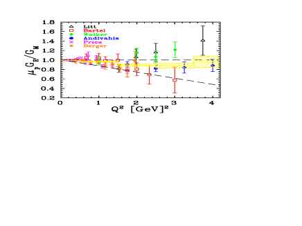
Figure 3: Ratio of electric to magnetic form factor from published Rosenbluth extractions Litt et al. (1970); Bartel et al. (1973); Walker et al. (1994); Andivahis et al. (1994); Price et al. (1971); Berger et al. (1971). The data are binned into five $Q^{2}$ bins, and the solid lines (shaded regions) represent the average (one-sigma range) for the measurement in each bin. The dashed lines indicate form factor scaling and the fit to the polarization transfer data.

While single experiment extractions avoid uncertainties arising from the relative normalization between different experiments, it should be noted that most of the form factor ratios shown in Fig. 3 do not correspond to single experiment extractions. Three of these six extractions Litt et al. (1970); Berger et al. (1971); Price et al. (1971) combine new cross section measurements with cross sections from one or more older experiments. In the extraction by Litt Litt et al. (1970) the new data are combined with results from three other experiments. While they give estimates of the effect of a small change in normalization, the quoted extractions of $G_{E_{p}}$ and $G_{M_{p}}$ ignore the normalization uncertainties. The extractions of Berger Berger et al. (1971) and Price Price et al. (1971) determine normalization factors between their data and previous experiments by comparing the cross sections from the different kinematics to the cross sections calculated assuming the dipole form for both $G_{E_{p}}$ and $G_{M_{p}}$, in effect assuming that form factor scaling is valid when determining the relative normalization factors. They do not apply any uncertainty associated with the determination of these normalization factors.

Two of the six extractions Bartel et al. (1973); Andivahis et al. (1994) use data from single experiments, but use different detectors to measure the large and small angle scattering. Bartel Bartel et al. (1973) does not determine a normalization factor, but quotes a 1.5% relative uncertainty between the small angle and large angle spectrometer data. Andivahis Andivahis et al. (1994) determined the relative normalization factor using data taken at identical kinematics for the SLAC 1.6 GeV and 8 GeV spectrometers. Unlike the cases where a normalization factor between two different experiments is determined, no assumption about the $\epsilon$-dependence goes into the determination. The uncertainty on the determination of the normalization factor was applied to the 1.6 GeV spectrometer which provided a single, low-$\epsilon$ point for each $Q^{2}$ value measured. However, the uncertainty related to the normalization (0.7% for Andivahis, 1.5% for Bartel) is common to all points, and will have an effect on $G_{E_{p}}/G_{M_{p}}$ that increases approximately linearly with $Q^{2}$ (for $Q^{2}\mathrel{\raise 1.29167pt\hbox{$>$}\mkern-14.0mu\lower 2.58334pt\hbox{$\sim$}}2$ GeV²). For the Andivahis measurement, this is roughly one-half the size of the total error, and so the entire data set could move up or down by roughly half of the total uncertainty shown in the figure. For the Bartel data, the high-$Q^{2}$ points all shift up or down by two-thirds of the total error due to a one-sigma shift in the normalization factor.

Only one of the experiments Walker et al. (1994) used a single detector for both small and large angle scattering, and is therefore free from normalization uncertainties. However, this is the experiment for which there was a correction for the small angle scattering that was not included in the analysis (Sect. III.1).

To study the consistency of the Rosenbluth measurements without the additional uncertainty caused by combining different experiments, one must examine only those experiments where an adequate range of $\epsilon$ was covered with a single detector in a single experiment. Five of the data sets from Table 1 cover an adequate range in $\epsilon$ to perform a single experiment L-T separation Walker et al. (1994); Litt et al. (1970); Berger et al. (1971); Andivahis et al. (1994); Janssens et al. (1966) . For these experiments, we have used only the cross section results from the primary measurement, with the updated radiative corrections as discussed in Sect. III.1.

Figure 4: Ratio of electric to magnetic form factor as extracted by the Rosenbluth technique, including only data sets where both forward and backward angle data were taken in the same apparatus (Table 2). The solid lines (shaded regions) indicate the average (one-sigma range) for the measurements in each bin. The dashed lines indicate form factor scaling and the fit to the polarization transfer data. The Janssens data has 19 $Q^{2}$ points, which have been rebinned to 10 data points.

Table 2 shows the values of $G_{E_{p}}/G_{\rm dipole}$, $G_{M_{p}}/G_{\rm dipole}$, and $\mu_{p}G_{E_{p}}/G_{M_{p}}$ from the reanalysis of the experiments that had adequate $\epsilon$ coverage. Higher order terms in the radiative corrections have been applied to those experiments which did not include these terms, as discussed in Section III.1.

Table 2: $G_{E_{p}}/G_{\rm dipole}$, $G_{M_{p}}/G_{\rm dipole}$, and $\mu_{p}G_{E_{p}}/G_{M_{p}}$ as extracted from the individual data sets shown in figure 4. A dipole mass of 0.71 GeV² is assumed for $G_{\rm dipole}$.

Data Set	$Q^{2}$	$G_{E_{p}}/G_{\rm dip}$	$G_{M_{p}}/G_{\rm dip}$	$\mu_{p}G_{E_{p}}/G_{M_{p}}$
	(GeV2)
Litt	1.499	1.180$\pm$0.339	0.982$\pm$0.111	1.201$\pm$0.481
Litt et al. (1970)	1.998	1.258$\pm$0.286	0.977$\pm$0.072	1.287$\pm$0.387
	2.500	1.106$\pm$0.164	1.010$\pm$0.028	1.095$\pm$0.192
	3.745	1.377$\pm$0.256	0.979$\pm$0.038	1.407$\pm$0.316
Walker	1.000	1.006$\pm$0.072	1.012$\pm$0.026	0.994$\pm$0.097
Walker et al. (1994)1	2.003	1.084$\pm$0.120	1.027$\pm$0.022	1.055$\pm$0.139
	2.497	0.944$\pm$0.180	1.045$\pm$0.022	0.903$\pm$0.191
	3.007	1.227$\pm$0.145	1.008$\pm$0.020	1.217$\pm$0.168
Andivahis	1.75	0.959$\pm$0.053	1.049$\pm$0.009	0.913$\pm$0.057
Andivahis et al. (1994)2	2.50	0.863$\pm$0.082	1.054$\pm$0.008	0.819$\pm$0.084
	3.25	0.868$\pm$0.185	1.047$\pm$0.015	0.829$\pm$0.188
	4.00	0.890$\pm$0.205	1.033$\pm$0.015	0.861$\pm$0.210
	5.00	0.578$\pm$0.453	1.030$\pm$0.016	0.561$\pm$0.448
Berger	0.389	0.938$\pm$0.025	0.985$\pm$0.019	0.952$\pm$0.043
Berger et al. (1971)	0.584	0.965$\pm$0.019	0.985$\pm$0.009	0.980$\pm$0.027
	0.779	0.950$\pm$0.041	1.004$\pm$0.012	0.946$\pm$0.051
	0.973	1.034$\pm$0.058	1.003$\pm$0.016	1.031$\pm$0.074
	1.168	1.074$\pm$0.132	1.022$\pm$0.023	1.051$\pm$0.152
	1.363	0.907$\pm$0.171	1.037$\pm$0.022	0.875$\pm$0.182
	1.557	1.229$\pm$0.265	1.031$\pm$0.027	1.192$\pm$0.285
	1.752	0.863$\pm$0.479	1.062$\pm$0.036	0.813$\pm$0.478
Janssens	0.156	1.021$\pm$0.028	0.926$\pm$0.027	1.103$\pm$0.057
Janssens et al. (1966)	0.179	0.962$\pm$0.024	0.959$\pm$0.016	1.003$\pm$0.039
	0.195	0.973$\pm$0.041	0.999$\pm$0.032	0.974$\pm$0.067
	0.234	1.020$\pm$0.034	0.939$\pm$0.025	1.087$\pm$0.061
	0.273	1.000$\pm$0.039	0.935$\pm$0.019	1.070$\pm$0.059
	0.292	1.005$\pm$0.044	0.936$\pm$0.022	1.074$\pm$0.068
	0.311	0.935$\pm$0.041	0.961$\pm$0.018	0.974$\pm$0.057
	0.389	1.014$\pm$0.041	0.956$\pm$0.016	1.061$\pm$0.058
	0.428	1.019$\pm$0.064	0.970$\pm$0.024	1.051$\pm$0.086
	0.467	0.993$\pm$0.055	0.974$\pm$0.020	1.020$\pm$0.073
	0.506	1.023$\pm$0.080	0.954$\pm$0.029	1.073$\pm$0.113
	0.545	0.984$\pm$0.069	0.983$\pm$0.020	1.000$\pm$0.087
	0.584	1.016$\pm$0.103	0.981$\pm$0.030	1.036$\pm$0.133
	0.623	0.951$\pm$0.085	0.987$\pm$0.020	0.964$\pm$0.103
	0.662	0.869$\pm$0.151	1.027$\pm$0.031	0.846$\pm$0.169
	0.701	1.076$\pm$0.100	0.982$\pm$0.021	1.096$\pm$0.121
	0.740	1.053$\pm$0.162	1.017$\pm$0.032	1.036$\pm$0.186
	0.779	0.805$\pm$0.160	1.035$\pm$0.022	0.778$\pm$0.169
	0.857	0.814$\pm$0.236	1.083$\pm$0.023	0.751$\pm$0.230
1 Data below 15 degrees excluded.
2 Using data from the 8 GeV spectrometer only.

The form factors from the single experiment extractions are given in Table 2, and the form factor ratios are plotted in Figure 4. The total $\chi^{2}$ is 18.2 for 25 degrees of freedom (d.o.f.). If the data below $Q^{2}=1.5$ GeV² are excluded, $\chi^{2}=10.3$ for 9 d.o.f. (33% CL). So, while the published extractions of the form factors from the different experiments have large scatter and yield somewhat inconsistent results, it is in part a result of the treatment of normalization factors in these extractions. The raw cross sections do not show this inconsistency, and the true single experiment extractions are consistent, and agree well with the global Rosenbluth analysis. Table 3 shows the $\chi^{2}$ value for each of these data sets compared to the new global fit to the cross section data (Fig. 5), and the polarization transfer parameterization of Ref. Gayou et al. (2002), i.e., Eqn. 4. Every data set except Janssens, which is limited to $Q^{2}<1$ GeV²), is in significantly better agreement with the global Rosenbluth analysis.

Table 3: $\chi^{2}$ of single experiment extractions compared to $G_{E_{p}}/G_{M_{p}}$ from global Rosenbluth analysis and polarization transfer ($0.6<Q^{2}<6.0$). Bartel is not included in the sum, as it is not taken from a single data set.

Data Set	data	$\chi^{2}$ (CL) vs.	$\chi^{2}$ (CL) vs.
	points	global Rosenbluth	polarization
Litt Litt et al. (1970)	4	5.39 (24.9%)	15.2 (0.43%)
Walker Walker et al. (1994)	4	5.56 (23.4%)	20.7 (0.04%)
Andivahis Andivahis et al. (1994)	5	1.44 (92%)	13.5 (1.9%)
Berger Berger et al. (1971)	6	2.91 (82%)	8.55 (20%)
Janssens Janssens et al. (1966)	6	3.74 (71%)	4.00 (68%)
Sum	25	19.1 (79%)	62.0 (0.006%)
Bartel Bartel et al. (1973)	8	6.35 (61%)	10.6 (23%)

We could include more data sets if we also used experiments where the forward and backward angle data are taken with different detectors, but where the normalization uncertainty is taken into account. If the Bartel and full Andivahis data sets are included, the results are still consistent ($\chi^{2}$=17.4 for 15 d.o.f. for $Q^{2}>1.5$ GeV²), and the average form factor ratio is again slightly below unity for the intermediate $Q^{2}$ values. However, because the uncertainty related to the normalization is common to all $Q^{2}$ values, the Bartel data does not strongly favor either scaling or the polarization transfer result, and the reduction in the error for Andivahis when both spectrometers are combined is largely offset by the introduction of the correlated error.

Because of the reduced data set and limited $\epsilon$ range caused by examining only single experiment extractions, the uncertainties are larger than for a global analysis. However, this data set should be free from the additional systematics related to the cross-experiment normalization. The extracted form factor ratio is slightly below scaling, in good agreement with the previous global analysis and in significant disagreement with the JLab polarization transfer results. In the next stage, we perform a global analysis of all of the cross section measurements to obtain the most precise result, and to test possible explanations of the discrepancy between the Rosenbluth and polarization measurements.

III.3 Fitting Procedure and Results

For the global fits to the cross section data, the form factors are parameterized using the same form as Refs. Bosted (1994); Brash et al. (2002):

$$G_{E}(q),G_{M}(q)/\mu_{p}=1~{}/~{}[1+p_{1}q+p_{2}q^{2}...+p_{N}q^{N}],$$ (6)

where $q=\sqrt{Q^{2}}$, and $N$ varies between 4 and 8; N=5 is adequate for a good fit. Because we wish to focus on the discrepancy at intermediate $Q^{2}$ values, we exclude data below $Q^{2}=0.6$ GeV², where the two techniques are in good agreement, and above $Q^{2}=8$ GeV², where the data do not allow for a Rosenbluth separation. Several parameterizations were tried, and this form was chosen because it provides enough flexibility to fit the $Q^{2}$-dependence of the form factors. This parameterization has odd powers of q, and so will not have the correct $Q^{2}\rightarrow 0$ behavior, but this is not relevant for this analysis, as we are focusing on the intermediate $Q^{2}$ range.

Figure 5: Ratio of electric to magnetic form factor from the new global fit (solid line), the Bosted fit Bosted (1994) (dashed line), and the fit to the polarization data (dotted line) Gayou et al. (2002).

In addition to the $2N$ parameters for the form factors, we also fit a normalization factor for each of the data sets. After partitioning the data sets for experiments that make multiple independent measurements, there are 20 normalization constants for the 16 experiments, as described in Sect. III.1. The fit parameters are allowed to vary, in order to minimize the $\chi^{2}_{\sigma}$, the total $\chi^{2}$ for the fit to the cross section data:

$$\chi^{2}_{\sigma}=\sum_{i=1}^{N_{\sigma}}\frac{(\sigma_{i}-\sigma_{\rm fit})^{2}}{(d\sigma_{i})^{2}}+\sum_{j=1}^{N_{\rm exp}}\frac{(\eta_{j}-1)^{2}}{(d\eta_{j})^{2}},$$ (7)

where $\sigma_{i}$ and $d\sigma_{i}$ are the cross section and error for each of the $N_{\sigma}$ data points, $\eta_{j}$ is the fitted normalization factor for the $j$th data set, and $d\eta_{j}$ is the normalization uncertainty for that data set. From the fit, we obtain the values of the fit parameters, $p_{i}$ (Eqn. 6), for both the electric and magnetic form factors, as well as the normalization factors for each of the 20 data sets. Figure 5 shows the result of our global fit along with the fit of Bosted Bosted (1994) to the previous global analysis and the fit to the polarization transfer data. While the modifications described in Sect. III.1 do decrease the $\mu_{p}G_{E_{p}}/G_{M_{p}}$ for $Q^{2}>2$ GeV², the new fit still gives a result that is well above the polarization transfer result at these momentum transfers. The $\chi^{2}$ value for this fit , obtained from Eqn. 7, is 162.0 for 198 d.o.f. (i.e., $\chi^{2}_{\nu}=0.818$).

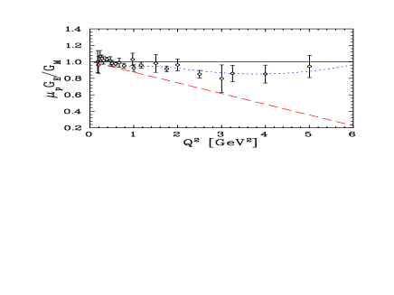
Figure 6: Ratio of electric to magnetic form factor as determined from direct L-T separations, using the normalizations determined from the global fit. The dotted line is the ratio from the global fit to $G_{E_{p}}$ and $G_{M_{p}}$, while the dashed line is the fit to the polarization measurements.

In order to estimate the uncertainty of the fit as a function of $Q^{2}$, we perform direct L-T separations wherever there are enough data points in a small range of $Q^{2}$. The normalization factors from the global fit are used to scale each data set, and the $Q^{2}$-dependence of the fit is used to scale each point to the central $Q^{2}$ value. Figure 6 shows the extracted ratios and uncertainties from these direct L-T separations at 26 $Q^{2}$ points up to 6 GeV² (15 above $Q^{2}$=0.6 GeV²). These $Q^{2}$ values are selected by requiring that five or more $\epsilon$ values are in each $Q^{2}$ bin, that the $\epsilon$-range of the data is at least 0.6, and that the correction required to scale the data points to the central $Q^{2}$ value never exceeds 2%. Due to this constraint on the correction, the resulting form factor ratio is independent of the model used to scale the cross sections for any reasonable model of the form factors.

To bring the data into agreement with the polarization transfer measurements, there would have to be a significant $\epsilon$-dependent error in the cross sections. Assuming that all of the data sets have such an error, and that it is linear in $\epsilon$, it would have to introduce an $\epsilon$-dependence of 5–6%, nearly independent of $Q^{2}$, for $Q^{2}\mathrel{\raise 1.29167pt\hbox{$>$}\mkern-14.0mu\lower 2.58334pt\hbox{$\sim$}}1.0$ GeV². This error would have to be even larger if it affected only some of the data sets, or if all of the uncertainty came at very large or very small values of $\epsilon$, e.g., if the error only occurred at very small angles or very low energies. In addition, a repeat of the above fit, excluding data at high ($\epsilon>0.8$) or low ($\epsilon<0.3$) values of $\epsilon$ did not have significant impact on the overall fit, changing the extracted values of $G_{E_{p}}$ by $<$5% for $Q^{2}$ values below 4 GeV². At higher $Q^{2}$ values, the cuts on $\epsilon$ led to larger changes in $G_{E_{p}}$, but the reduction in the $\epsilon$ range did not allow for a precise extraction of $G_{E_{p}}$, and the changes were small compared to the final uncertainty.

III.4 Consistency Checks

As a first check of the consistency of the data sets, we examine the contribution to the total $\chi^{2}$ coming from each data set. No data set had an excessively large $\chi^{2}$ value, only five of the data sets have $\chi^{2}_{\nu}>1$ and all five of these have reasonable confidence levels (none below 10%). In addition, no individual cross section value had excessively large ($>3\sigma$) deviations from the fit. However, the fact that the fit gives such a low $\chi^{2}_{\nu}$ value, combined with the fact that most of the individual data sets have $\chi^{2}_{\nu}<1$, indicates that several data sets may have overly conservative estimates for the uncertainties. Therefore, the total $\chi^{2}$ value of the global fits cannot be viewed as an absolute measure of goodness of fit, and we will focus on the change in $\chi^{2}$ between different fits when using the same data sets as a measure of the ${\it relative}$ goodness of fit.

While these statistical measures help us locate individual data sets that are inconsistent with the bulk of the data, they are not always enough to detect systematic errors in the data, especially when the error estimates are somewhat conservative. It is quite possible that these statistical measures will overlook systematic errors which are small compared to the individual uncertainties, but still large enough to modify the small $\epsilon$-dependence extracted. Thus, we would also like to look for any systematic trends in the data sets which might modify the result.

For each data set we compare the measured cross sections to the fit and look for systematic deviations from the global fit as a function of $Q^{2}$, $\theta$, $E_{e}^{\prime}$ or $\epsilon$. A systematic $\epsilon$-dependence of just 1–2% may not show up in the total $\chi^{2}$ of the data set (especially if the errors are overly conservative or are noticeably larger than 1–2%), but could lead to a noticeable change in the electric form factor at high $Q^{2}$ values. In the preliminary version of the global fit, it was observed that the Walker data Walker et al. (1994) showed a clear deviation from the global fit at small angles (Fig. 7), even though the $\chi^{2}$ value for this data set was quite reasonable. The data below 20^∘ was then removed from later fits.

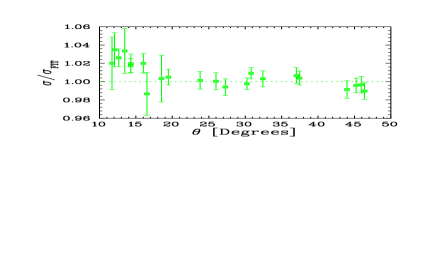
Figure 7: Ratio of cross section to global fit for Walker data Walker et al. (1994), showing a systematic deviation at low scattering angles.

Similarly, the Goitein data Goitein et al. (1970) showed a systematic deviation from the initial global fit. The ratio of cross section from this data set to that obtained from the global fit was systematically higher by $\mathrel{\raise 1.29167pt\hbox{$>$}\mkern-14.0mu\lower 2.58334pt\hbox{$\sim$}}5$% for the higher $Q^{2}$ values. The original publication listed several differences in the larger $Q^{2}$ data: different collimation, additional cuts, and several corrections which were negligible for the low $Q^{2}$ data were quite large for these points. Because of the difference in running conditions between low and high $Q^{2}$, it was decided to break up this data set into two subsets, each with its own normalization factor, and to increase the normalization uncertainty from 2.8% to 3.8% for the large $Q^{2}$ data due to the larger and less well understood corrections for this data set. The high $Q^{2}$ data could also have been excluded altogether, but while the conditions for this subset of the data were different, there was no clear evidence of any specific problem.

As another check for systematic trends in the data, we examine the direct L-T separations performed at several values of $Q^{2}$. For the separations shown in Fig. 6, we plot the cross sections versus $\epsilon$ to look for systematic deviations from the expected linearity and to look for data sets which have systematic differences in their $\epsilon$-dependence. After separating the Goitein data into a two subsets the only data set which stands out is the data from Janssens Janssens et al. (1966), which has some deviations from a linear $\epsilon$-dependence. Sometimes the higher $\epsilon$ points are above the extracted (linear) $\epsilon$-dependence, sometimes they are below, and sometimes they just show non-statistical scatter. Because there are no systematic trends to these deviations, and because there was no indication of problems in the original publication, we do not exclude this data set from the analysis. The effects of excluding specific data sets was tested separately, and the results are presented in the following section.

III.5 Bad Data Sets?

Because most of the high $Q^{2}$ Rosenbluth data comes from a limited set of experiments, it is possible that a single data set may have an error that strongly biases the global analysis. The global fit described in Sect. III.3 was repeated 20 times, with a different data set excluded each time. The exclusion of a single data set generally had little effect on the global fit, although there were a few data sets whose exclusion lead to a noticeable increase (up to $\sim 10$% for $Q^{2}>2$ GeV²) or a noticeable decrease in $\mu_{p}G_{E_{p}}/G_{M_{p}}$ (from 5% to 15% for $3<Q^{2}<5$ GeV²). Even excluding two or three data sets together generally had little effect on the result. The three data sets whose exclusion lead to the greatest decrease in the ratio were identified, and the fit was repeated with all three excluded. Figure 8 shows the result of the full global fit, and the global fit with all three of these data sets removed. There is little change for $Q^{2}<3$ GeV², where both techniques have high precision, while there is a significant decrease for $Q^{2}>3$ GeV², where the ratio is constrained by a very limited set of experiments and is very poorly constrained when the three data sets are removed. Also, while the ratio at large $Q^{2}$ is significantly decreased, it is still well above the polarization transfer result.

Figure 8: Ratio of electric to magnetic form factor from the global fit of all of the data sets (solid curve), and the lowest ratio found by excluding up to three of the data sets (dashed curve). Also shown is the fit to the polarization data (dotted line).

III.6 Consistency of Global Fit and Polarization Transfer Results

The new global fit is clearly in disagreement with the polarization transfer results, and shows no indications of inconsistency between the data sets or bias due to inclusion of erroneous results. One remaining possibility is that it is the fitting procedure itself, rather than the data, that leads to this discrepancy. While we include the relative normalization factors for the experiments in the analysis and obtain best-fit values for the normalizations, it is possible that a small change in the normalization factors for some or all of the experiments would significantly improve the agreement with the polarization transfer data without dramatically increasing the overall $\chi^{2}$ of the fit.

To test this possibility, we performed a constrained fit, using the same data as in the previous fit, but fitting only $G_{M_{p}}$ and the normalization factors, while fixing the ratio $\mu_{p}G_{E_{p}}/G_{M_{p}}$ to the fit of the polarization transfer data (Eqn. 4). The extracted magnetic form factor is roughly 2% higher over the entire $Q^{2}$ range ($Q^{2}\mathrel{\raise 1.29167pt\hbox{$>$}\mkern-14.0mu\lower 2.58334pt\hbox{$\sim$}}1$ GeV²), due to the reduction in strength from the electric contribution. The constrained fit has 5 more degrees of freedom (the parameters that were used to fit $G_{E_{p}}$) while the total $\chi^{2}$ for the fit increases by 40.2 (from $\chi^{2}$=162.0 for 198 d.o.f. to $\chi^{2}$=202.2 for 203 d.o.f.).

Even though the normalization factors are adjusted in order to best reproduce the polarization transfer results, the direct L-T separation using these normalization factors is systematically high for all $Q^{2}$ values, as seen in figure 9. So not only is this fit significantly worse, the normalization factors derived from constraining the $G_{E_{p}}/G_{M_{p}}$ ratio to match polarization transfer data still do not fully explain the magnitude of the falloff of $G_{E_{p}}/G_{M_{p}}$. The effect is only slightly less using the combined fit to all four recoil polarization data sets. With the ratio forced to $\mu_{p}G_{E_{p}}/G_{M_{p}}=1-0.135(Q^{2}-0.24)$ (Eqn. 5), the total $\chi^{2}$ is 197.3, an increase of 35.3 in the total $\chi^{2}$, with 5 extra degrees of freedom.

Because of the conservative error estimates on some of the data sets, the reduced $\chi^{2}$ is still less than one, even after this noticeable increase. Therefore, the absolute value of $\chi^{2}_{\nu}$ cannot be directly used to measure goodness of fit. To get an idea of the relative goodness of fit, one can scale the overall uncertainties on the cross sections such that $\chi^{2}_{\nu}$ for the unconstrained fit is approximately one. This means reducing the cross section uncertainties by a factor of 0.905, leading to $\chi^{2}_{\nu}$=1 for the unconstrained fit to the cross section data, $\chi^{2}_{\nu}$=1.22 (1.9% CL) for the fit constrained to Eqn. 4, and $\chi^{2}_{\nu}$=1.19 (3.5% CL) for the fit constrained to Eqn. 5. Assuming that the unconstrained fit should yield $\chi^{2}_{\nu}=1$ is arbitrary, but it is a reasonable staring point since we expect $\chi^{2}_{\nu}\approx 1$ if the estimated uncertainties are correct and if our fitting function can accurately reproduce the data. One would expect $\chi^{2}$ to be even higher, and the confidence levels for the constrained fits to be even lower, if the fitting function does not adequately reproduce the data or if there are any inconsistencies in the cross sections. So it is likely that these confidence levels are upper limits of the consistency between the cross section data and the parameterizations of the polarization transfer data.

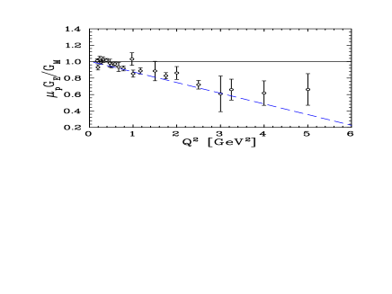
Figure 9: Ratio of electric to magnetic form factor as determined from direct L-T separations, using the normalization factors determined by forcing the ratio to reproduce the polarization transfer fit (dashed line). Although the normalization factors were fitted to reproduce the polarization transfer results, the direct L-T separation is systematically higher than the fit at large $Q^{2}$ values.

Forcing the fit to match the parameterization of the polarization transfer data gives too much weight to polarization data, as it neglects the uncertainties in the polarization measurements. To avoid this, we also performed a combined fit, treating the cross section and polarization transfer measurements on an equal footing. We repeated the procedure described in Section III.3, but with the inclusion of the polarization transfer ratios as additional data points, and with a systematic offset included for each data set Jones et al. (2000); Gayou et al. (2001, 2002), as in the fit from section II.2 (Eqn. 5). The $\chi^{2}$ for this combined fit is the contribution from the cross section measurements (Eqn. 7) plus the additional contribution from the polarization transfer ratio measurements:

$$\chi^{2}=\chi^{2}_{\sigma}+\sum_{k=1}^{N_{R}}\frac{(R_{k}-R_{\rm fit})^{2}}{(dR_{\rm stat})^{2}}+\sum_{l=1}^{N_{\rm exp}}\frac{(\Delta_{l})^{2}}{(dR_{\rm sys})^{2}}$$ (8)

where $R=\mu_{p}G_{E_{p}}/G_{M_{p}}$, $dR_{\rm stat}$ and $dR_{\rm sys}$ are the statistical and systematic uncertainties in $R$, $N_{R}$ is the total number of polarization transfer measurements of $R$, $\Delta_{l}$ is the offset for each data set, and $N_{\rm exp}$ is the number of polarization transfer data sets. Because the polarization transfer data are included in the fit, the normalization factors for the cross section measurements are adjusted to give consistency between different cross section data sets, as well as consistency with the polarization measurements of $\mu_{p}G_{E_{p}}/G_{M_{p}}$, much as they are in the constrained fit.

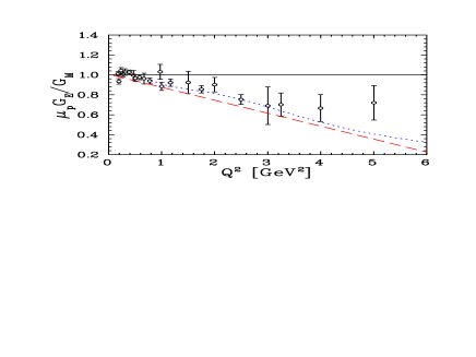
Figure 10: Ratio of electric to magnetic form factor as determined from combined fit of cross section and polarization transfer data. The dotted line is the result of the fit, and the circles are the results from the direct L-T separations using the normalization factors determined from the global fit.

The ratio of $G_{E_{p}}/G_{M_{p}}$ for this combined fit is systematically higher then the polarization transfer results (Fig. 10). As with the constrained fit, the direct L-T separations using the normalization factors from this global fit are systematically higher than the actual ratio obtained in the fit, and the quality of fit is significantly reduced when the polarization transfer data is included: $\chi^{2}=215.8$ for 218 d.o.f., an increase in $\chi^{2}$ of 53.8 for the additional 20 data points.

While the combined fit to cross section and polarization transfer data yields a ratio that is close to the polarization measurements, this does not imply that the data sets are yielding consistent results, just that the polarization transfer results dominate the fit. The goodness of fit is significantly worse when the polarization transfer data is added to the cross section measurements. Because of the conservative errors, it is difficult to estimate the relative goodness-of-fit for the combined fit. We can scale the uncertainties by a factor of 0.905 to force $\chi^{2}_{\nu}=1$ for the fit to cross sections, yielding $\chi^{2}_{\nu}=1.21$ (1.9% CL) for the combined fit to the cross sections and polarization transfer. However, as discussed for the constrained fit, this is likely to be an upper limit on the consistency of the two fits. The comparison of single experiments L-T separations to the polarization transfer fit, $\mu_{p}G_{E_{p}}/G_{M_{p}}=1-0.13(Q^{2}-0.04)$, yields a confidence level of 0.006% (Table 3). To take into account the uncertainties of the polarization transfer measurements, we compare the single experiment L-T separations to the fit with the slope parameter decreased by one sigma, i.e., $\mu_{p}G_{E_{p}}/G_{M_{p}}=1-0.125(Q^{2}-0.04)$ Brash et al. (2002). This gives $\chi^{2}=57.8$ for 25 degrees of freedom, or a 0.02% confidence level.

We can also use a recently-proposed test to determine the consistency of the data from the two techniques, following the prescription of Refs. Maltoni and Schwetz (2003); Maltoni et al. (2002). They define a test called the “parameter goodness-of-fit” (PG) measure, which is designed test the consistency of independent data sets sharing a common set of parameters. This approach is significantly less sensitive to over- or underestimates of the uncertainties of the individual data sets. The corresponding $\chi^{2}$ for this test, $\overline{\chi^{2}}_{\rm min}$, is the increase in $\chi^{2}$ for a combined fit, relative to fits of the individual data sets. The effective number of degrees of freedom is the number of parameters in common between the two data sets, which in this case are the parameters that go into the ratio. So, for comparison of the cross section and polarization transfer results, $\overline{\chi^{2}}_{\rm min}$ is the difference between $\chi^{2}_{\rm min}$ for the combined fit and the values of $\chi^{2}_{\rm min}$ for the independent fits of the cross section data and of the polarization transfer data, i.e., $\overline{\chi^{2}}_{\rm min}=215.8-162.0-26.5=27.3$. Note that the $\chi^{2}$ for the fit to polarization transfer data alone is not the result presented in section II.2, because the combined fit includes only the polarization transfer data from JLab Jones et al. (2000); Gayou et al. (2001, 2002). The two types of data both constrain the ratio, effectively 5 parameters, and so the PG goodness-of-fit measure corresponds to $\overline{\chi^{2}}_{\rm min}=27.3$ for 5 degrees of freedom, or a 0.005% CL. This measure has two advantages over the confidence levels calculated based on the direct comparison of the single experiment extractions to the polarization transfer fits. It includes the entire cross section data set, rather than just the five single experiments extractions in Table 3, and it accounts for the uncertainties of the both the cross section and polarization transfer measurements.

In the end, both approaches yield a confidence level of $\ll 1\%$, showing that the data sets are clearly inconsistent. If it is an error in the cross section data, it would take an $\epsilon$-dependent correction of at least 5–6% to make the results from the two techniques consistent. Until the source of the inconsistency between the two data sets is determined, we do not know how to combine the measurements in order to obtain a reliable extraction of the form factors.

IV Discussion

We have presented a new extraction of the proton electromagnetic form factors based on a global analysis of elastic cross section data at moderate to high $Q^{2}$. The extracted value for $G_{E_{p}}/G_{M_{p}}$ is slightly lower than in the previous global analysis Walker et al. (1994); Bosted (1994), but is still well above the values determined by polarization transfer measurements. We have demonstrated that the discrepancy between the global Rosenbluth analysis and the polarization transfer results is not merely the result of the inclusion of one or two bad data sets. While modifying the normalization factors of the different experiments can lead to a significant reduction in the extracted $G_{E_{p}}/G_{M_{p}}$, they yield significantly lower quality fits, and still do not fully resolve the discrepancy between the two techniques. Finally, we have demonstrated that the apparent inconsistency between single experiment extractions is not due to any inconsistency in the data themselves, but due to improper treatment of normalization uncertainties when combining data from multiple measurements. The values of $G_{E_{p}}/G_{M_{p}}$ from single experiment extractions, which avoid the normalization uncertainties involved in a combined analysis, are self-consistent and in good agreement with the result of the global analysis.

This indicates that there is a more fundamental reason for the discrepancy, such as an intrinsic problem with either the Rosenbluth or polarization transfer techniques, or an error in the cross section or polarization transfer measurements. If the error is in the cross section measurements, it must be a systematic problem that yields a similar $\epsilon$-dependence in a large set of these measurements: a 5–6% linear $\epsilon$-dependence in all cross section measurements above $Q^{2}\approx 1$ GeV², larger if only some of the data are affected, or if the error has significant deviations from a linear $\epsilon$-dependence. Since the the cross sections are necessary to extract the absolute value of $G_{E_{p}}$ and $G_{M_{p}}$ even with very precise measurements of $G_{E_{p}}/G_{M_{p}}$, an unknown systematic error in the cross section measurements implies unknown systematic errors in the values of the form factors.

Until this discrepancy is understood, it is premature to dismiss the Rosenbluth extractions of the form factors. There is a significant difference in the values of $G_{E_{p}}$ extracted by these two techniques, and smaller ($\sim$3%) differences in the extracted values of $G_{M_{p}}$. In addition to the impact this uncertainty has on the state of our knowledge of the proton structure, it also affects other measurements which rely on the proton electromagnetic form factors as input, or measurements where there are significant corrections due to the radiative tail of the elastic peak.

While the cross sections extracted using the new polarization transfer ratio measurements are typically within a few percent of previous parameterizations, the large change in the ratio of the form factors means that the changes in extracted cross sections are strongly $\epsilon$-dependent. Thus, it will have a significant impact on experiments that try to examine a small $\epsilon$-dependence. For example, there will be a large effect on Rosenbluth separation measurements for $A(e,e^{\prime})$ (e.g., Coulomb sum rule measurements at large $q$) or $A(e,e^{\prime}p)$ (e.g., $>50$% difference for recent results for separated structure functions in nuclei Dutta et al. (2000, )).

Experiments which need only the unseparated elastic cross sections are less sensitive to these uncertainties. Two such examples are the extraction of the axial form factors from neutrino scattering measurements, and extractions of nucleon spectral functions in nuclei, which use the proton electromagnetic form factors (or elastic cross sections) as input. An analysis of the neutrino measurements Budd and Bodek shows that the extracted axial form factor is essentially identical using the Rosenbluth or polarization transfer parameterizations of the form factors. The difference also has relatively little effect on the extraction of the spectral function in unseparated $A(e,e^{\prime}p)$ measurements. This is not surprising, as the polarization measurements only determine the relative contributions from $G_{E_{p}}$ and $G_{M_{p}}$, and the overall size of the form factors is still determined by fitting the cross section measurements. With the constraint from the polarization measurements included, the combined fit can reproduce the measured cross sections at the few percent level. However, while fits with and without polarization transfer data can reproduce the measured cross sections at the few percent level, the discrepancy in the ratio of form factors implies that some large set of these cross sections may be wrong by 5% or more. Until the source of the discrepancy is identified, there is no way to be sure which of these cross sections are incorrect, or how well these cross sections are measured.

Finally, it is important to note that the while a consistent extraction of $G_{E_{p}}$ and $G_{M_{p}}$ yields only small differences in the elastic cross sections, this is not always the case when combining extractions of $G_{E_{p}}$ and $G_{M_{p}}$ from different analyses. Using the polarization transfer data to constrain $G_{E_{p}}/G_{M_{p}}$ and cross section measurements to determine the size of $G_{E_{p}}$ and $G_{M_{p}}$, as presented here or in another recent analysis Brash et al. (2002), yields cross sections that are nearly identical to those from the cross section analysis only, except for a change of approximately 5% in their $\epsilon$-dependence. However, using $G_{M_{p}}$ as extracted from Rosenbluth extractions, combined with $G_{E_{p}}/G_{M_{p}}$ from polarization transfer measurements can yield cross sections which are significantly lower than the measured cross sections. For example, if one takes the magnetic form factor parameterization from Bosted Bosted (1994), but calculates the electric form factor using the polarization transfer ratios, the resulting cross sections are lower by 4–10% over a very large $Q^{2}$ range (0.1–15 GeV²), compared to using both form factors from the Bosted parameterization. Thus, it is extremely important to use a consistently determined set of form factors when examining the difference between the Rosenbluth and polarization transfer data, or when parameterizing the elastic cross section for comparison to other data or calculations.

There have been two more recent L-T separations from Hall C at JLab, which were not included in this analysis. One took points at $Q^{2}$=0.64 and 1.81 GeV² Dutta et al. , both of which were in agreement with the new global Rosenbluth analysis presented here (Fig. 5). A more extensive set of Rosenbluth measurements was taken as part of JLab experiment E94-110 Keppel et al. (1994). The experiment measured $R=\sigma_{L}/\sigma_{T}$ in the resonance region, but also took elastic data. This allowed them to perform several Rosenbluth separations for $0.5<Q^{2}<5.5$ GeV² Christy et al. . These results are also in excellent agreement with the new global fit presented here. While these newer JLab measurements have not been included in the new fit, the fact the single experiment extractions from these measurements are in good agreement with the global fit indicates that they would not significantly change the final fit, although their inclusion would decrease the uncertainties in the global analysis, and thus increase the significance of the discrepancy with the polarization transfer results.

V Summary and Future Outlook

A careful analysis of Rosenbluth extractions has been performed to test the consistency of the worlds body of elastic cross section measurements, and to test explanations for the discrepancy between polarization transfer and Rosenbluth extractions of the proton form factors. We find no inconsistency in the cross section data sets, and cannot remove the discrepancy via modifications of the relative normalization of different data sets or the exclusion of individual measurements.

This discrepancy indicates a fundamental problem in one of the two techniques, or a significant error in either the polarization transfer or cross section measurements. An error in the polarization data would imply a large error in the electric form factor extracted from a combined analysis, and may have consequences for other recoil polarization measurements. An error in the cross section data would have to introduce an $\epsilon$-dependence of $>5$% for $Q^{2}>1$ GeV², implying an error in both the electric and magnetic form factors However, while the uncertainty in the form factors is smaller in this case, the error in the cross section measurements will also lead to uncertainties in other measurements which require the elastic cross section as input. Thus, even if it is demonstrated that the polarization transfer measurements are correct, it is necessary to determine the source of the discrepancy in order to have confidence in our knowledge of the elastic cross sections, and any other measurement which relies on this knowledge.

Future results from JLab should significantly improve the situation. JLab experiment E01-001 ran in 2002, and performed a high precision Rosenbluth separation using a modified experimental technique Arrington et al. (2001); Arrington (2002). This experiment should be able to clearly differentiate between the ratio of $G_{E_{p}}/G_{M_{p}}$ as seen in previous Rosenbluth measurements and in the polarization transfer results, while being significantly less sensitive to the types of systematics that are the dominant sources of uncertainties in previous results. In addition, there is an approved experiment to extend the polarization transfer measurements to higher $Q^{2}$ Perdrisat et al. (2001) using a different spectrometer from the previous measurements ($Q^{2}>1$ GeV²), which all used the High Resolution Spectrometer in Hall A at JLab. This will provide the first independent check of the Hall A large $Q^{2}$ polarization transfer experiments, whose systematics are dominated by the spin-precession in the spectrometer. These tests will provide crucial information to help explain the discrepancy in the measurements of the proton form factors. The resolution of the discrepancy will significantly improve the state of knowledge of the proton form factors, as well as determining if other other measurements utilizing the Rosenbluth or polarization transfer techniques are affected.