A model for consecutive spallation and fragmentation reactions in inverse kinematics at relativistic energies

Abstract

Secondary reactions induced by relativistic beams in inverse kinematics in a thick target are relevant in several fields of experimental physics and technology, like secondary radioactive beams, production of exotic nuclei close to the proton drip line, and cross-section measurements for applications of spallation reactions for energy production and incineration of nuclear wastes. A general mathematical formulation is presented and successively applied as a tool to disentangle the primary reaction yields from the secondary production in the measurement of fission of a ²³⁸U projectile impinging on a proton target at the energy of 1 A GeV.

PACS: 25.40.Sc; 25.70.Mn; 25.85.Ge; 25.85.-w; 24.10.-i; 29.25.-t; 29.30.Aj
keywords: SECONDARY AND MULTIPLE REACTIONS IN INVERSE KINEMATICS; In-flight identification in Z and A by magnetic spectrometer, Measured primary spallation and fragmentation cross sections; Fission and evaporation residues cross sections; Spallation reaction, p(²³⁸U,X), E=1 AGeV; Relevance for the production of radioactive beams.

, , ,

1 Introduction

The reaction residues of projectile spallation and fragmentation, produced with heavy-ion beams can undergo consecutive nuclear reactions in the target. The secondary reaction production, especially by the use of a thick target, can extend towards exotic nuclei, which would not be generated in the primary reaction. The induction of multiple reactions in thick targets is also a technique to obtain exotic beams. On the other hand, in the measurements dedicated to the extraction of formation cross sections, the secondary reactions enter in competition with the primary production and are a disturbing process. In this work we will refer to a recent measurement of the isotopic production cross section in the reaction ²³⁸U+p at 1 A GeV [1, 2, 3]. The experiment was performed in inverse kinematics with the high-resolution magnetic spectrometer FRS [4] (GSI, Darmstadt) directing the uranium beam on a hydrogen target. The target thickness was optimised in order to maximize the primary production rate in respect to parasitic reactions and to limit the average share of secondary reactions to values of about $5\%$. This share and its uncertainty enters in the total experimental uncertainty; though, some of the measured isotopes, suffer from a much larger competition of the secondary reactions.

When the primary isotopic production extends over a wide neutron-number range, as it will be pointed out, we can not extract reliable cross sections in the neutron-deficient side. Especially for the fission residues, the approaching towards the residue corridor defines a limit for the measurement technique: in this case the neutron-deficient isotopes will reveal to be mostly or entirely produced by secondary spallation of fission residues.

The beginning of the present work is dedicated to the derivation of the mathematical formalism to treat consecutive reactions in a general form, independently of any application. Furthermore, we will focus on the cross-section measurement, and an analytical recipe to disentangle the secondary contribution from the primary production is presented. The method has been successfully applied in the data analysis of the reaction ²³⁸U+p at 1 A GeV.

2 Derivation of the exact formulation for multiple reactions

2.1 Attenuation of the beam

When a beam of ions characterised by atomic number ${\mathrm{Z}}_{0}$ and neutron number ${\mathrm{N}}_{0}$ interacts with a layer of matter, the intensity ${\cal I}_{0}$ evolves accordingly to the total reaction cross-section of the projectile $\sigma_{0}=\sigma({\mathrm{N}}_{0}{\mathrm{Z}}_{0})$ and the properties of the target, like the density $\rho\,[g\,cm^{-3}]$ and the mass of the target nuclei $A_{\mathrm{tar}}\,[g]$. The loss $-\mathrm{d}{\cal I}_{0}(\xi)$ of the beam intensity is proportional to the path $\mathrm{d}\xi$ traversed inside of the target medium and to the intensity ${\cal I}_{0}(\xi)$ reached at the position $\xi$ in the beam direction:

$$-\mathrm{d}{\cal I}_{0}(\xi)\,=\,a_{\scriptstyle\mathrm{tar}}\sigma_{0}\cdot{\cal I}_{0}(\xi)\mathrm{d}\xi.$$

The target properties are represented by $a_{\mathrm{tar}}\,[cm^{-1}mb^{-1}]$ $=$ $10^{-27}\cdot{\cal N_{\scriptscriptstyle A}}\cdot\rho/A_{\mathrm{tar}}$, with ${\cal N_{\scriptscriptstyle A}}$ indicating the Avogadro’s number. Integrating over the whole path $x$ we obtain the probability for the projectile $({\mathrm{N}}_{0}{\mathrm{Z}}_{0})$ to survive for a path $x$ in the layer of matter as

$${\cal P}_{0}({\mathrm{N}}_{0}{\mathrm{Z}}_{0},\chi)\,=\,{\cal I}_{0}(x)/{\cal I}_{0}(0)\,=\,e^{\displaystyle-\sigma_{0}a_{\scriptstyle\mathrm{tar}}x}\,=\,e^{\displaystyle-\sigma_{0}\chi},$$ (1)

where $\chi\,[mb^{-1}]=a_{\scriptstyle\mathrm{tar}}x$ indicates the number of target atoms per $10^{-27}cm^{2}$.

2.2 Probability of primary reaction

The probability for the projectile $({\mathrm{N}}_{0}{\mathrm{Z}}_{0})$ to interact with the target in a path length $\mathrm{d}\xi$ with a total reaction cross-section $\sigma_{0}$ and produce a residue $({\mathrm{N}}_{1}{\mathrm{Z}}_{1})$ with a probability $p_{(0\to 1)}$ is defined as

$$\mathrm{d}{P}({\mathrm{N}}_{0}{\mathrm{Z}}_{0},{\mathrm{N}}_{1}{\mathrm{Z}}_{1},\mathrm{d}\xi)\,=\,a_{\scriptstyle\mathrm{tar}}\mathrm{d}\xi\cdot\sigma_{0}\cdot p_{(0\to 1)}\,=\,\mathrm{d}\zeta\cdot\sigma_{(0\to 1)},$$

where $\sigma_{(0\to 1)}=\sigma_{0}\cdot p_{(0\to 1)}$ results to be the production cross section for the reaction $({\mathrm{N}}_{0}{\mathrm{Z}}_{0}\to{\mathrm{N}}_{1}{\mathrm{Z}}_{1})$, and $\mathrm{d}\zeta=a_{\scriptstyle\mathrm{tar}}\mathrm{d}\xi$ is the number of atoms in a layer of matter defined by the path $\mathrm{d}\xi$ per $10^{-27}cm^{2}$. The total probability for the projectile $({\mathrm{N}}_{0}{\mathrm{Z}}_{0})$ to react only once in the target in any position $\xi$ and produce the observed fragment $({\mathrm{N}}_{1}{\mathrm{Z}}_{1})$ is expressed by the probability for the projectile to survive for a path $\xi$, react in $\mathrm{d}\xi$ and produce a residue that will traverse the remaining length of the target without any further reaction; as pictured in the drowing below, this expression should be integrated over any path $\xi$ in the form :

$$\begin{split}&\int_{0}^{x}\left[{\cal P}_{0}({\mathrm{N}}_{0}{\mathrm{Z}}_{0},\xi)\cdot\mathrm{d}{P}({\mathrm{N}}_{0}{\mathrm{Z}}_{0},{\mathrm{N}}_{1}{\mathrm{Z}}_{1},d\xi)\cdot{\cal P}_{0}({\mathrm{N}}_{1}{\mathrm{Z}}_{1},x{\scriptstyle-}\xi)\right]\,=\\ &\qquad=\sigma_{(0\to 1)}e^{\displaystyle-\sigma_{1}\chi}\int_{0}^{\chi}{\cal P}_{0}({\mathrm{N}}_{0}{\mathrm{Z}}_{0},\zeta)\,e^{\displaystyle\sigma_{1}\zeta}\,\mathrm{d}\zeta.\end{split}$$

Introducing Eq. (1) in the integral, the solution expressed in terms of target thickness gives:

$${\cal P}_{1}({\mathrm{N}}_{0}{\mathrm{Z}}_{0},{\mathrm{N}}_{1}{\mathrm{Z}}_{1},\chi)\,=\,-\sigma_{(0\to 1)}\left(\frac{e^{\displaystyle-\sigma_{0}\chi}}{\sigma_{0}-\sigma_{1}}+\frac{e^{\displaystyle-\sigma_{1}\chi}}{\sigma_{1}-\sigma_{0}}\right).$$ (2)

2.3 Secondary reactions

After the primary reaction of the beam occurred, we should consider the possibility for a further interaction of the residues with the target. In this case, in order to obtain the probability of observing a secondary fragment ${\mathrm{N}}_{2}{\mathrm{Z}}_{2}$, the quantity to integrate over any path through the target in beam direction is the product of three terms: the probability for the beam to undergo a primary reaction during the path $\xi$ and produce the intermediate fragment ${\mathrm{N}}_{1}{\mathrm{Z}}_{1}$, the probability for a further reaction $({\mathrm{N}}_{1}{\mathrm{Z}}_{1}\to{\mathrm{N}}_{2}{\mathrm{Z}}_{2})$ in the interval $\mathrm{d}\xi$, and the probability that the final residue survives for the remaining path $x-\xi$. This description is represented below in the drawing and it results into the following equation:

$$\begin{split}&\int_{0}^{x}\bigl{[}{\cal P}_{1}({\mathrm{N}}_{0}{\mathrm{Z}}_{0},{\mathrm{N}}_{1}{\mathrm{Z}}_{1},\xi)\cdot\mathrm{d}{P}({\mathrm{N}}_{1}{\mathrm{Z}}_{1},{\mathrm{N}}_{2}{\mathrm{Z}}_{2},d\xi)\cdot{\cal P}_{0}({\mathrm{N}}_{2}{\mathrm{Z}}_{2},x{\scriptstyle-}\xi)\bigr{]}\,=\\ &\qquad=\displaystyle\sigma_{(1\to 2)}\,e^{\displaystyle-\sigma_{2}\chi}\int_{0}^{\chi}{\cal P}_{1}({\mathrm{N}}_{0}{\mathrm{Z}}_{0},{\mathrm{N}}_{1}{\mathrm{Z}}_{1},\zeta)\,e^{\displaystyle\sigma_{2}\zeta}\,\mathrm{d}\zeta.\end{split}$$

Introducing Eq. (2) in the integral we obtain for the secondary reactions:

$$\begin{split}&{\cal P}_{2}({\mathrm{N}}_{0}{\mathrm{Z}}_{0},{\mathrm{N}}_{1}{\mathrm{Z}}_{1},{\mathrm{N}}_{2}{\mathrm{Z}}_{2},\chi)=\\ &\quad=\displaystyle\sigma_{(0\to 1)}\sigma_{(1\to 2)}\biggl{[}\displaystyle\frac{e^{\displaystyle-\sigma_{0}\chi}}{(\sigma_{0}{\scriptstyle-}\sigma_{1})(\sigma_{0}{\scriptstyle-}\sigma_{2})}+\frac{e^{\displaystyle-\sigma_{1}\chi}}{(\sigma_{1}{\scriptstyle-}\sigma_{0})(\sigma_{1}{\scriptstyle-}\sigma_{2})}+\frac{e^{\displaystyle-\sigma_{2}\chi}}{(\sigma_{2}{\scriptstyle-}\sigma_{0})(\sigma_{2}{\scriptstyle-}\sigma_{1})}\biggr{]}.\end{split}$$ (3)

As it will be demonstrated in the section A.1, the procedure followed so far to obtain the probability for secondary reactions can be extended to higher orders according to the recursive relation:

$$\begin{split}&{\cal P}_{n}({\mathrm{N}}_{0}{\mathrm{Z}}_{0},{\mathrm{N}}_{1}{\mathrm{Z}}_{1},\cdots,{\mathrm{N}}_{n}{\mathrm{Z}}_{n},\chi)\,=\\ &\quad=\,\displaystyle\sigma_{(n-1\to n)}e^{\displaystyle-\sigma_{n}\chi}\int_{0}^{\chi}{\cal P}_{n-1}({\mathrm{N}}_{0}{\mathrm{Z}}_{0},{\mathrm{N}}_{1}{\mathrm{Z}}_{1},\cdots,{\mathrm{N}}_{n-1}{\mathrm{Z}}_{n-1},\zeta)\,e^{\displaystyle\sigma_{n}\zeta}\,\mathrm{d}\zeta.\end{split}$$ (4)

Repeating the iterative integral for higher and higher orders we obtain the solution for the $n^{\mathrm{th}}$order:

$${\cal P}_{n}({\mathrm{N}}_{0}{\mathrm{Z}}_{0},{\mathrm{N}}_{1}{\mathrm{Z}}_{1},\cdots,{\mathrm{N}}_{n}{\mathrm{Z}}_{n},\chi)\,=\,(-1)^{n}\,\underset{\scriptscriptstyle i=1}{\overset{\scriptscriptstyle n}{\textstyle\prod}}\sigma_{(i-1\to i)}\,\sum_{i=0}^{n}\frac{e^{\displaystyle-\sigma_{i}\chi}}{\underset{\scriptscriptstyle j=0\atop j\neq i}{\overset{\scriptscriptstyle n}{\prod}}(\sigma_{i}-\sigma_{j})}.$$ (5)

3 A more stable approximated formulation

If we neglect the technical and chemical properties of the target, i.e. we consider the target homogeneous and a full acceptance of the spectrometer, the relation (5) is formally rigorous and exact. Nevertheless, it should be observed that the term $(\sigma_{i}-\sigma_{j})$ could generate instability in numerical calculations: when very few mass is removed in one step of the chain of consecutive reactions, the total cross-sections $\sigma_{i}$ and $\sigma_{j}$ become almost identical, and the denominator $(\sigma_{i}-\sigma_{j})$ becomes very small. In this case, the sum in Eq. (5) remains finite but its numerical computation can be problematic in this form.

A possibility to remove this inconvenience is to perform a series of consecutive $1^{\mathrm{st}}$-order approximations in iterating the integration (4). We start applying the approximation to the Eq. (2), which describes the probability of primary reaction:

$${\cal P}_{1}({\mathrm{N}}_{0}{\mathrm{Z}}_{0},{\mathrm{N}}_{1}{\mathrm{Z}}_{1},\chi)\,=\,-\sigma_{(0\to 1)}\frac{e^{\displaystyle-\sigma_{0}\chi}-e^{\displaystyle-\sigma_{1}\chi}}{\sigma_{0}-\sigma_{1}}.$$

Expanding the exponential to the $2^{\mathrm{nd}}$ order in $(\sigma_{0}-\sigma_{i})\chi$, we obtain the simpler relation:

$${\cal P}_{1}({\mathrm{N}}_{0}{\mathrm{Z}}_{0},{\mathrm{N}}_{1}{\mathrm{Z}}_{1},\chi)\,\approx\,\sigma_{(0\to 1)}\,\chi\,e^{\displaystyle-\frac{\sigma_{0}+\sigma_{1}}{2}\chi}.$$ (6)

Integrating Eq. (6) by the relation (4) we obtain the probability of observing a secondary product generated by a given intermediate fragment in the following form:

$$\sigma_{(0\to 1)}\sigma_{(1\to 2)}\,e^{\displaystyle-\sigma_{2}\chi}\int_{0}^{\chi}\zeta e^{\displaystyle-\left(\frac{\sigma_{0}+\sigma_{1}}{2}-\sigma_{2}\right)\zeta}\mathrm{d}\zeta.$$

Expanding to the $1^{\mathrm{st}}$ order in $\frac{1}{2}\left(\sigma_{0}+\sigma_{1}\right)\chi-\sigma_{2}\chi$, integrating, and isolating $\chi^{2}/2$, we obtain the approximated form of the Eq. (3) in the $1^{\mathrm{st}}$ order :

$$\begin{split}&{\cal P}_{2}({\mathrm{N}}_{0}{\mathrm{Z}}_{0},{\mathrm{N}}_{1}{\mathrm{Z}}_{1},{\mathrm{N}}_{2}{\mathrm{Z}}_{2},\chi)\,\approx\,\sigma_{(0\to 1)}\sigma_{(1\to 2)}\,\frac{\chi^{2}}{2}\,e^{\displaystyle-\frac{\sigma_{0}+\sigma_{1}+\sigma_{2}}{3}\,\chi}.\end{split}$$ (7)

Physically, this relation can be intuitively pictured as “one-third-target approximation”, as the argument of the exponential represents the attenuation of the beam, the primary and the secondary residue, respectively, when they cross a third of the target.

Iterating the integration (4) followed by the first order expansion in respect to the argument of the exponential, we obtain the approximation for $n$ consecutive reactions, equivalent to dividing the target in $n$ portions of equal thickness, each one originating a successive reaction with a probability $\sigma_{(i-1\to i)}\chi/i$:

$${\cal P}_{n}({\mathrm{N}}_{0}{\mathrm{Z}}_{0},{\mathrm{N}}_{1}{\mathrm{Z}}_{1},\cdots,{\mathrm{N}}_{n}{\mathrm{Z}}_{n},\chi)\, = \,\underset{\scriptscriptstyle i=1}{\overset{\scriptscriptstyle n}{\textstyle\prod}}\left(\frac{\sigma_{(i-1\to i)}\;\chi}{i}\right)\,e^{\displaystyle-\frac{{\textstyle\sum_{j=0}^{n}}\,\sigma_{j}}{n+1}\,\chi}$$ (8)

$$= \,\underset{\scriptscriptstyle i=1}{\overset{\scriptscriptstyle n}{\textstyle\prod}}\sigma_{(i-1\to i)}\,\frac{\chi^{n}}{n!}\,e^{\displaystyle-\frac{{\textstyle\sum_{j=0}^{n}}\,\sigma_{j}}{n+1}\,\chi}.$$

To obtain the Eq. (8) we can follow the prescription presented in the section A.2.

4 Measured reaction probability

Besides the production rate in the target expressed in Eq. (5) , the measured production rate of an isotope NZ should also take into account the probability that the residue NZ is observed outside of the target, and is detected in the spectrometer. The measured probability to produce NZ can be written for a given chain of intermediate products as

$${\cal M}_{n}({\mathrm{N}}_{0}{\mathrm{Z}}_{0},\cdots,{\mathrm{N}}_{n}{\mathrm{Z}}_{n},\chi)\,=\,{\cal P}_{n}({\mathrm{N}}_{0}{\mathrm{Z}}_{0},\cdots,{\mathrm{N}}_{n}{\mathrm{Z}}_{n},\chi)\cdot t_{n}({\mathrm{N}}_{1}{\mathrm{Z}}_{1},\cdots,{\mathrm{N}}_{n}{\mathrm{Z}}_{n}),$$

where $t_{n}$ is the transmission coefficient depending on the kinematics of all the intermediate isotopes: it depends on the instrumental device and it represents the probability that a fragment with a given velocity is transmitted through the spectrometer. The transmission is a key parameter in the measurement of fission products which are only partially accepted, as some of the residues are emitted with large angle and hit the pipe of the spectrometer. The measured probability to obtain NZ by multiple reactions accounts for the sum of the orders of the reactions, that is the superposition of the contributions of primary, secondary and multiple reactions evaluated for any possible choice of intermediate fragments

$${\cal M}({\mathrm{N}}_{0}{\mathrm{Z}}_{0},{\mathrm{N}}{\mathrm{Z}},\chi)\,=\,\sum_{\mathrm{order}\,n}\,\sum_{n-1\,\mathrm{chain}}{\cal M}_{n}({\mathrm{N}}_{0}{\mathrm{Z}}_{0},\cdots,{\mathrm{N}}_{n}{\mathrm{Z}}_{n},\chi),$$

where the first sum accounts for the order of reactions and the second sum accounts for an order given for all the possible chains of successive $n-1$ intermediate fragments leading from the initial projectile ${\mathrm{N}}_{0}{\mathrm{Z}}_{0}$ to the observed residue NZ. We can express the whole relation in terms of cross-sections if we introduce the apparent cross section

$$\tilde{\sigma}_{({\mathrm{N}}_{0}{\mathrm{Z}}_{0}\to{\mathrm{N}}{\mathrm{Z}})}(\chi)=\frac{1}{\chi}\frac{{\cal M}({\mathrm{N}}_{0}{\mathrm{Z}}_{0},{\mathrm{N}}{\mathrm{Z}},\chi)}{t({\mathrm{N}}{\mathrm{Z}})},$$

where $t({\mathrm{N}}{\mathrm{Z}})$ is the transmission factor of the spectrometer. It is derived from the measured spectrum of longitudinal velocities, by assuming the emission isotropic in respect to the centre of mass; this assumption allows to evaluate the angular distribution of the fragments and the fraction which is selected by the angular acceptance. Due to the difference in the distributions of the emission velocities related to fission fragments or evaporation residues, respectively , the coefficient $t({\mathrm{N}}{\mathrm{Z}})$ depends strongly on the dominant reaction process responsible for the production of a given isotope NZ. In order to have a more complete description of the reaction process, we can disentangle fission residues from evaporation residues. If we assume that fission could occur only once in a chain of successive reactions we obtain the general description:

$$\tilde{\sigma}_{({\mathrm{N}}_{0}{\mathrm{Z}}_{0}\to{\mathrm{N}}{\mathrm{Z}})}(\chi)\,\,=\,\,\frac{1}{\chi}\,\sum_{\mathrm{order}\,n}\,\,\sum_{n-1\,\mathrm{chain}}\,\left\{\left[{\cal R}_{n}^{\scriptstyle\mathrm{evr}}{\cal T}_{n}^{\scriptstyle\mathrm{evr}}+\sum_{j=N_{1}Z_{1}}^{j=NZ}\left({\cal R}_{n}^{\scriptstyle\mathrm{evr},\atop\scriptstyle\mathrm{fis}j}{\cal T}_{n}^{\scriptstyle\mathrm{evr},\atop\scriptstyle\mathrm{fis}j}\right)\right]\,{\cal A}_{n}\right\},$$ (9)

with:

$${\cal R}_{n}^{\scriptstyle\mathrm{evr}}\,=\,\frac{1}{n!}\,\prod_{i={\mathrm{N}}_{1}{\mathrm{Z}}_{1}}^{i={\mathrm{N}}{\mathrm{Z}}}(\sigma_{i-1\to i}^{\scriptstyle\mathrm{evr}}\chi)\qquad,\qquad{\cal R}_{n}^{\scriptstyle\mathrm{evr},\atop\scriptstyle\mathrm{fis}j}\,=\,\frac{1}{n!}\,\sigma_{j-1\to j}^{\scriptstyle\mathrm{fis}}\chi\prod_{\scriptstyle i={\mathrm{N}}_{1}{\mathrm{Z}}_{1}\atop\scriptstyle i\neq j}^{i={\mathrm{N}}{\mathrm{Z}}}(\sigma_{i-1\to i}^{\scriptstyle\mathrm{evr}}\chi),$$

$$\begin{split}{\cal T}_{n}^{\scriptstyle\mathrm{evr}}&\,=\,\frac{t_{n}^{\scriptstyle\mathrm{evr}}({\mathrm{N}}_{1}{\mathrm{Z}}_{1},{\mathrm{N}}_{2}{\mathrm{Z}}_{2},\cdots,{\mathrm{N}}_{n-1}{\mathrm{Z}}_{n-1},{\mathrm{N}}{\mathrm{Z}})}{t({\mathrm{N}}{\mathrm{Z}})},\\ {\cal T}_{n}^{\scriptstyle\mathrm{evr},\atop\scriptstyle\mathrm{fis}j}&\,=\,\frac{t_{n}^{\scriptstyle\mathrm{evr},\atop\scriptstyle\mathrm{fis}j}({\mathrm{N}}_{1}{\mathrm{Z}}_{1},{\mathrm{N}}_{2}{\mathrm{Z}}_{2},\cdots,{\mathrm{N}}_{n-1}{\mathrm{Z}}_{n-1},{\mathrm{N}}{\mathrm{Z}})}{t({\mathrm{N}}{\mathrm{Z}})},\end{split}$$

$$\begin{split}{\cal A}_{n}({\mathrm{N}}_{0}{\mathrm{Z}}_{0},{\mathrm{N}}_{1}{\mathrm{Z}}_{1},\cdots,{\mathrm{N}}_{n}{\mathrm{Z}}_{n},\chi)\,&=\,(-1)^{n}\,n!\,\sum_{i=0}^{n}\frac{e^{\displaystyle-\sigma_{i}\chi}}{\underset{\scriptscriptstyle j=0\atop j\neq i}{\overset{\scriptscriptstyle n}{\prod}}(\sigma_{i}\chi-\sigma_{j}\chi)}\,\approx\,e^{\displaystyle-\frac{{\textstyle\sum_{j=0}^{n}}\,\sigma_{j}\chi}{n+1}}.\end{split}$$

The first sum describes the apparent cross-section as a composition of consecutive orders of multiple reactions. The second sum over all the possible intermediate fragments can be represented by an expansion in $(n-1)$ chains, the $i^{\mathrm{th}}$ one satisfying the condition $({\mathrm{N}}_{i-1}+{\mathrm{Z}}_{i-1})\geq({\mathrm{N}}_{i}+{\mathrm{Z}}_{i})\geq({\mathrm{N}}_{i+1}+{\mathrm{Z}}_{i+1})$: each successive intermediate fragment should in fact have lower mass but not necessarily lower charge due to the charge exchange. Nevertheless, since this process has very low cross section, the condition can be safely decomposed into ${\mathrm{N}}_{i-1}\geq{\mathrm{N}}_{i}\geq{\mathrm{N}}_{i+1}$ and ${\mathrm{Z}}_{i-1}\geq{\mathrm{Z}}_{i}\geq{\mathrm{Z}}_{i+1}$ for each sum $i$. ${\cal R}_{n}^{\scriptstyle\mathrm{evr}}$ and ${\cal R}_{n}^{\scriptstyle\mathrm{evr},\,\scriptstyle\mathrm{fis}j}$ are the terms defining the reaction chain: ${\cal R}_{n}^{\scriptstyle\mathrm{evr}}$ is the term representing the series of reactions producing NZ as a chain of consecutive evaporation residues; ${\cal R}_{n}^{\scriptstyle\mathrm{evr},\,\scriptstyle\mathrm{fis}j}$ differs from the former one because at the step $j$ a fission reaction occours. Due to the very low fissility of the fission residues, the probability to undergo two consecutive fission reactions is negligible: therefore, we imposed only one possible fission event in the chain. The terms ${\cal T}_{n}^{\mathrm{evr}}$ and ${\cal T}_{n}^{\scriptstyle\mathrm{evr},\,\scriptstyle\mathrm{fis}j}$ are transmission coefficients ratios and depend on the optics of the instrumental device; a more detailed description of these coefficients will follow in the next paragraph. ${\cal A}_{n}$ is the term describing the attenuation of each nucleus traversing the target, either the beam-like projectile and the consecutive residues. It should be observed that this terms takes into consideration also the attenuation of the final residue, due to the probability to undergo a reaction of order $n+1$; nevertheless no reaction of order $n+1$ appears in the term describing the reaction chain. As discussed in the previous paragraph, according to the possibility to have an unstable solution, it is important to decide in which condition the exact form containing the term $\sigma_{i}-\sigma_{j}$ and referred to in Eq. (5) can be applied; it could be safer to use the approximated form represented by the Eq. (8) which remains valid as long as the products $(\sigma_{i}-\sigma_{j})\chi$ are small compared to unity.

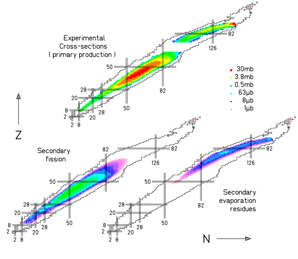
Figure 1: Top. Experimental cross-sections for the reaction ²³⁸U+p at 1 A GeV [1, 2, 3] measured in inverse kinematics and corrected for the secondary contribution. A hydrogen target of thickness $87.3\,mg/cm^{2}$ was used. Bottom. Contribution of the secondary reactions to the appearent cross section as calculated with Eq. (9). The secondary production is more than one order of magnitude lower than the primary production. The secondary fission residues, shown on the left, account for primary evaporation residues followed by secondary fission residues or primary fission residues followed by secondary evaporation residues. The primary evaporation residues followed by secondary evaporation residues are shown on the right.

We simulated the secondary and ternary production (expressed as apparent cross-sections) in the reaction of ²³⁸U at $1$A GeV impinging on a target of hydrogen of $87.3\,10^{-3}[\mathrm{g}/\mathrm{cm}^{2}]$ by solving the system (9) with the choice of the approximated form (8). The production cross-sections $\sigma_{{\mathrm{N}}_{0}{\mathrm{Z}}_{0}\to{\mathrm{N}}_{i}{\mathrm{Z}}_{i}}^{\scriptstyle\mathrm{evr}}$ and $\sigma_{{\mathrm{N}}_{0}{\mathrm{Z}}_{0}\to{\mathrm{N}}_{i}{\mathrm{Z}}_{i}}^{\scriptstyle\mathrm{fis}}$ were measured experimentally in inverse kinematics at the FRagment Separator in Darmstadt [1, 2, 3]. The total cross-sections $\sigma_{i}$ have been calculated numerically according to the model of Karol-Brohm [5, 6], very well suited for proton reactions. Another choice would be the formula of Benesh et al. [7], where the total cross-section is calculated neglecting the energy of the projectile and the nuclear properties of the target: as a consequence of these approximations the description of ion-proton reactions gives an almost-systematic over-prediction of around 20% in the total cross section; nevertheless, in the case of ion-ion reactions, the formula of Benesh et al. gives satisfactory results and is then preferable due to the lower computing time.

Figure 2: Study of the evolution of the mass distribution of the residues generated in the reaction ²³⁸U+p at 1 A GeV for different orders of multiple reactions in a hydrogen target of thickness $87.3mg/cm^{2}$. The primary production corresponds to the experimental (dots) cross sections [1, 2, 3] corrected for the secondary contribution. Nine elements from Tb to Ta are still not analysed and their cross sections are replaced by a calculation performed with the codes BURST [8] and ABLA-PROFI [9, 10, 11] coupled together. The secondary and ternary production is calculated according to Eq. (9). The calculation has been performed using both the exact form (dots) of the term $\mathcal{A}_{n}$ and the approximation of equally-partitioned target (histogram) described in Eq. (8); the perfect overlapping of the two calculations assures the reliability of the approximation.

The fundamental parameters to enter in the system of Eq. (9) in order to obtain a physical description of multiple reactions are the production cross sections $\sigma_{i-1\to i}^{\scriptstyle\mathrm{evr}}$ and $\sigma_{i-1\to i}^{\scriptstyle\mathrm{fis}}$. Due to the enormous number of these parameters, a very fast numerical calculation is needed. The best solution we found is to couple a parameterisation to obtain the hot prefragments with a physical fission-evaporation code.

Figure 3: Evolution of the isotopic distributions for different orders of multiple reactions in the reaction ²³⁸U+p at 1 A GeV. The different productions have been obtained as discussed in fig. (1) and in fig. (2). Evaporation residues (top): The mean neutron number of elements close to the projectile like Fr are not affected by consecutive reactions, while a shift towards lower neutron-numbers appears for elements like Os, produced in the light side of the mass-distribution slope. Fission residues (bottom): The isotopic distribution of multiple-reaction products is deformed and the mean neutron number tends to move towards the residue corridor (dashed line).

The routine BURST (applied for the correction for secondary reaction in the analysis presented in [8]) was chosen to reproduce the intra-nuclear cascade. The evaporation-stage has been simulated with the statistical de-excitation code ABLA [9, 10] and the fission code PROFI [11]. Also the possibility of multifragment emission, in the case of light and highly excited systems, has been taken into account and simulated according to the reference [12]. The resulting isotopic production probability has then been normalized to the total reaction cross section obtained with the model of Karol-Brohm.

We verified that the results fit well with the available data of proton-reactions for ²³⁸U [1, 2, 3] and ²⁰⁸Pb [8] at $1$ A GeV and ¹⁹⁷Au [13, 14] at $800$ A MeV. In fig. (1) the result of the calculation for ²³⁸U+p at $1$ A GeV is shown. The primary production is represented by the experimental cross sections; due to the competition between fission and evaporation residues, nine elements (from Tb to Ta) have not yet been analysed; for the calculation, this gap has been filled with model-deduced cross sections. It should be noted that in this figure we anticipate the result on the experimental primary production cross section, that have been disentangled from the secondary contribution by applying the procedure described in the following section. The secondary yields are one to two orders of magnitude lower than the primary production as shown in fig. (2). The secondary evaporation residues are expected to extend to lighter masses and slightly overlap with the heavier fission products. In general, even if the mean neutron number of the isotopic distribution does not change significantly in respect to the primary evaporation residues, we observe an increased production of neutron-loss channels and an extension of the isotopic distribution towards the proton-rich side. In contrast to the case of evaporation residues, the secondary fission residues are evidently less neutron rich. This is almost exclusively due to secondary evaporation residues that reduce the primary heavy neutron-rich fission products and populate the neutron deficient side; this is shown in fig. (3). The ternary production, three to four orders of magnitude lower than the primary production, shows an even more enhanced production around the residue corridor. The production resulting from secondary and ternary reactions, could be increased using a thicker target than the one considered in the present calculation.

5 A recipe to disentangle primary and secondary reactions

The calculation presented in fig. (1) derives from the direct solution of the system of equations (9), applied to the measured reaction cross section of ²³⁸U$+$p at $1$ A GeV. Evidently, the result of the experiment was the cumulative detection of the primary production together with the secondary, without any clear experimental indication about how to select the primary yields. Thus, the primary-reaction cross section were disentangled from the secondary contribution solving the system (9) inversely.

From the calculation shown in fig. (2), we confirm that the ternary contribution induced by a thin target is even lower than the uncertainties of the data introduced by the measurement, and it can be safely neglected. In this case, the notation has been changed in respect to Eq. (9). The index “fis,evr” defines primary fission residues leading to secondary evaporation residues, “evr,fis” defines primary evaporation residues undergoing secondary fission and “evr,evr” primary evaporation residues producing secondary evaporation residues. This consideration justifies the reduction of the system (9) to the second order of consecutive reactions only. Thus, we can write the matrix relation

$${\tilde{\cal X}}^{\scriptstyle\mathrm{evr}} ={\cal L}^{\scriptstyle\mathrm{evr}}{\cal X}^{\scriptstyle\mathrm{evr}}+{\cal G}^{\scriptstyle\mathrm{evr},\scriptstyle\mathrm{evr}}{\cal X}^{\scriptstyle\mathrm{evr}}$$ (10)

$${\tilde{\cal X}}^{\scriptstyle\mathrm{fis}}\; ={\cal L}^{\scriptstyle\mathrm{fis}}{\cal X}^{\scriptstyle\mathrm{fis}}+{\cal G}^{\scriptstyle\mathrm{fis},\scriptstyle\mathrm{evr}}{\cal X}^{\scriptstyle\mathrm{evr}}+{\cal G}^{\scriptstyle\mathrm{evr},\scriptstyle\mathrm{fis}}{\cal X}^{\scriptstyle\mathrm{fis}},$$ (11)

where $\tilde{\cal X}$ is the vector of apparent cross sections directly measured by the experiment and $\cal X$ is the set of the unknown primary cross sections that we intend to extract:

$${\tilde{\cal X}}=\left(\begin{array}[]{c}{\tilde{\sigma}}_{({\mathrm{N}}_{0}{\mathrm{Z}}_{0}\to{\mathrm{N}}_{0}{\mathrm{Z}}_{0})}(\chi)\\ {\tilde{\sigma}}_{({\mathrm{N}}_{0}{\mathrm{Z}}_{0}\to{\mathrm{N}}_{0-1}{\mathrm{Z}}_{0})}(\chi)\\ \vdots\\ {\tilde{\sigma}}_{({\mathrm{N}}_{0}{\mathrm{Z}}_{0}\to{\mathrm{N}}{\mathrm{Z}})}(\chi)\\ \vdots\\ \end{array}\right)\quad,\quad{\cal X}=\left(\begin{array}[]{c}\sigma_{({\mathrm{N}}_{0}{\mathrm{Z}}_{0}\to{\mathrm{N}}_{0}{\mathrm{Z}}_{0})}\\ \sigma_{({\mathrm{N}}_{0}{\mathrm{Z}}_{0}\to{\mathrm{N}}_{0-1}{\mathrm{Z}}_{0})}\\ \vdots\\ \sigma_{({\mathrm{N}}_{0}{\mathrm{Z}}_{0}\to{\mathrm{N}}{\mathrm{Z}})}\\ \vdots\\ \end{array}\right).$$ (22)

The elements

$$\alpha_{{\mathrm{N}}{\mathrm{Z}}}=\frac{1}{2}\;{\cal A}_{1}({\mathrm{N}}_{0}{\mathrm{Z}}_{0},{\mathrm{N}}{\mathrm{Z}},\chi)$$

$$\beta_{{\mathrm{N}}_{i}{\mathrm{Z}}_{i}}=\frac{1}{2}\;\sigma_{({\mathrm{N}}_{i}{\mathrm{Z}}_{i}\to{\mathrm{N}}{\mathrm{Z}})}\chi\,{\cal A}_{2}({\mathrm{N}}_{0}{\mathrm{Z}}_{0},{\mathrm{N}}_{i}{\mathrm{Z}}_{i},{\mathrm{N}}{\mathrm{Z}},\chi)\,{\cal T}_{2}({\mathrm{N}}_{i}{\mathrm{Z}}_{i},{\mathrm{N}}{\mathrm{Z}})$$ (23)

are collected into the diagonal matrix ${\cal L}$ and the triangular matrix ${\cal G}$ respectively :

$${\displaystyle\cal L}=\scriptsize\left(\begin{array}[]{ccccc}\alpha_{{\mathrm{N}}_{0}{\mathrm{Z}}_{0}}&&&&\\ &\alpha_{{\mathrm{N}}_{0-1}{\mathrm{Z}}_{0}}&&&\\ &&\ddots&&\\ &&&\alpha_{{\mathrm{N}}{\mathrm{Z}}}&\\ &&&&\ddots\\ \end{array}\right)\;\;,\;\;{\cal G}=\scriptsize\left(\begin{array}[]{ccccccc}\beta_{{\mathrm{N}}_{0}{\mathrm{Z}}_{0}}&&&&&&\\ \beta_{{\mathrm{N}}_{0}{\mathrm{Z}}_{0}}&\beta_{{\mathrm{N}}_{0-1}{\mathrm{Z}}_{0}}&&&&&\\ \\ \vdots&&&\ddots&&&\\ \\ \beta_{{\mathrm{N}}_{0}{\mathrm{Z}}_{0}}&\ldots&\beta_{{\mathrm{N}},{\mathrm{Z}}+1}&\ldots&\beta_{{\mathrm{N}}+1,{\mathrm{Z}}}&\beta_{{\mathrm{N}}{\mathrm{Z}}}&\\ \vdots&&&&&&\ddots\\ \end{array}\right).$$ (36)

The terms $\beta_{{\mathrm{N}}_{i}{\mathrm{Z}}_{i}}$ are evaluated for any of the involved secondary reaction through a model calculation of each intermediate cross section $\sigma_{({\mathrm{N}}_{i}{\mathrm{Z}}_{i}\to{\mathrm{N}}{\mathrm{Z}})}$. The attenuation terms ${\cal A}_{1}$ and ${\cal A}_{2}$, contained in $\alpha_{{\mathrm{N}}{\mathrm{Z}}}$ and in $\beta_{{\mathrm{N}}_{i}{\mathrm{Z}}_{i}}$, respectively, are obtained by the calculation of the total reaction cross sections $\sigma_{i}$ through a model. The transmission coefficient ratios ${\cal T}_{2}({\mathrm{N}}_{i}{\mathrm{Z}}_{i},{\mathrm{N}}{\mathrm{Z}})$ are calculated for any combination of intermediate residue ${\mathrm{N}}_{i}{\mathrm{Z}}_{i}$ and final residue NZ as explained at the end of the present section.

The Eq. (10) describes the measured evaporation-residue yields as the sum of two contributions: the quantity ${\cal L}^{\scriptstyle\mathrm{evr}}$ represents the loss of primary cross-section due to the attenuation in the target. The term ${\cal G}^{\scriptstyle\mathrm{evr},\scriptstyle\mathrm{evr}}$ is the gain factor, which takes into account the increasing of the yields due to the residues produced in two consecutive evaporation-residue steps. The Eq. (11) refers to the fission-like yields, i.e. the production-rate of those residues which the measurement attributes to fission events according to the kinematical identification. The apparent fission cross-section suffers from the attenuation in the target, expressed by the term ${\cal L}^{\scriptstyle\mathrm{fis}}$, and from two sources of gain: secondary evaporation residues of fission residues, represented by ${\cal G}^{\scriptstyle\mathrm{fis},\scriptstyle\mathrm{evr}}$ and evaporation residues followed by fission events, as described by ${\cal G}^{\scriptstyle\mathrm{evr},\scriptstyle\mathrm{fis}}$. In the case of evaporation residues, the loss term depletes the yields of the elements close to the projectile. Part of these losses are redistributed by the gain factor ${\cal G}^{\scriptstyle\mathrm{evr}}$ and populate the tail of light evaporation residues. The effect of this process results into reducing the slope of the mass distribution of the evaporation residues. Another part of the losses goes into the term ${\cal G}^{\scriptstyle\mathrm{evr},\scriptstyle\mathrm{fis}}$, estabilishing a coupling between the Eq. (10) and the Eq. (11) and populates the fission yields with secondary fission fragments. Since the primary evaporation residues that could undergo a secondary fission event should be rather close to the projectile, the reaction products should preserve essentially the structure of the primary fission residues and do not introduce any modification or displacement in the original primary distribution. This is no more true when the primary reaction is a fission event. In this case, the losses are redistributed by the gain factor ${\cal G}^{\scriptstyle\mathrm{fis},\scriptstyle\mathrm{evr}}$ as secondary evaporation residues of primary fission residues. The effect of this process is a strong deformation of the fission-fragment distribution. The primary fission products which, in general, are neutron-rich are turned by secondary reactions into evaporation residues, generally neutron deficient, and have the tendency to cumulate around the residue corridor. As a consequence, the whole fission distribution appears less neutron-rich in the measurement than it is expected in reality. Moreover, the steeper is the slope of the fission distribution in the neutron-deficient side, the higher is the probability that some residues are produced by secondary reactions in that region.

An example of the reaction mechanism ending up into the production of a secondary fission residue is illustrated in fig. (4), where the isotopic distribution of the formation cross section of ¹¹⁰Pd and ¹⁰⁰Pd for each possible intermediate mother nucleus is presented.

Figure 4: Representation of the intermediate fragments ${\mathrm{N}}_{i}{\mathrm{Z}}_{i}$ that, once produced as residues of the reaction ²³⁸U+p at 1 A GeV, react a second time in the target and produce either ¹⁰⁰Pd (left) or ¹¹⁰Pd (right). On the isotopic chart we represent the secondary production cross sections for all the possible reactions ${\mathrm{N}}_{i}{\mathrm{Z}}_{i}\to^{100}$Pd or ${\mathrm{N}}_{i}{\mathrm{Z}}_{i}\to^{110}$Pd, multiplied by $\sigma_{{}^{238}\mathrm{U}\to{\mathrm{N}}_{i}{\mathrm{Z}}_{i}}$ and divided by the total production cross section for the primary residues of ²³⁸U. As clearly shown in the Z-projection, while the secondary production of neutron rich ¹¹⁰Pd can be equally attributed to fission or to evaporation residues of the neighbouring elements, the secondary production of the less neutron rich ¹⁰⁰Pd can be prevalently attributed to evaporation residues of elements lighter than Nd.

We deduce that the stable and neutron-rich ¹¹⁰Pd is produced with high cross section mostly by primary fission of heavy fragments, and its formation as a secondary residue should not enter in competition with its production by primary reactions. Inversely, the secondary formation of ¹⁰⁰Pd, close to the residue corridor, results to depend almost exclusively on secondary evaporation of the primary fission fragments: the measured yield of formation of ¹⁰⁰Pd should then be rather different from its primary production cross-section.

Thanks to the triangularity of the matrix ${\cal G}$, the system can be solved iteratively by the recurrence relation:

$$\sigma_{({\mathrm{N}}_{0}{\mathrm{Z}}_{0}\to{\mathrm{N}}{\mathrm{Z}})}^{\mathrm{evr}}\,\,=\,\,\frac{1}{\alpha_{{\mathrm{N}}{\mathrm{Z}}}^{evr}}\biggl{(}{\tilde{\sigma}}^{\mathrm{evr}}_{({\mathrm{N}}_{0}{\mathrm{Z}}_{0}\to{\mathrm{N}}{\mathrm{Z}})}-\sum_{{\mathrm{N}}_{i}\geq{\mathrm{N}}\atop{\mathrm{Z}}_{i}\geq{\mathrm{Z}}}\sigma_{({\mathrm{N}}_{0}{\mathrm{Z}}_{0}\to{\mathrm{N}}_{i}{\mathrm{Z}}_{i})}^{\mathrm{evr}}\beta_{{\mathrm{N}}_{i}{\mathrm{Z}}_{i}}^{evr}\biggr{)}.$$ (37)

A similar equation holds for $\sigma_{({\mathrm{N}}_{0}{\mathrm{Z}}_{0}\to{\mathrm{N}}{\mathrm{Z}})}^{\mathrm{fis}}$. Introducing the expressions  (23) in Eq. (37) and substituting the term ${\cal A}_{2}$ in the approximated form we obtain the recursive relation:

$$\begin{split}&\sigma_{({\mathrm{N}}_{0}{\mathrm{Z}}_{0}\to{\mathrm{N}}{\mathrm{Z}})}^{\scriptstyle\mathrm{evr}}\quad=\quad{\tilde{\sigma}}^{\scriptstyle\mathrm{evr}}_{({\mathrm{N}}_{0}{\mathrm{Z}}_{0}\to{\mathrm{N}}{\mathrm{Z}})}\,e^{\displaystyle\frac{\chi}{2}(\sigma_{{\mathrm{N}}_{0}{\mathrm{Z}}_{0}}+\sigma_{{\mathrm{N}}{\mathrm{Z}}})}+\\ &\quad-\frac{\chi}{2}\sum_{{\mathrm{N}}_{i}\geq{\mathrm{N}}\atop{\mathrm{Z}}_{i}\geq{\mathrm{Z}}}\biggl{[}\sigma_{({\mathrm{N}}_{0}{\mathrm{Z}}_{0}\to{\mathrm{N}}_{i}{\mathrm{Z}}_{i})}^{\scriptstyle\mathrm{evr}}\sigma_{({\mathrm{N}}_{i}{\mathrm{Z}}_{i}\to{\mathrm{N}}{\mathrm{Z}})}^{\scriptstyle\mathrm{evr}}{\cal T}_{2}^{\scriptstyle\mathrm{evr,}\atop\scriptstyle\mathrm{evr}}({\mathrm{N}}_{i}{\mathrm{Z}}_{i},{\mathrm{N}}{\mathrm{Z}})\,e^{\displaystyle\frac{\chi}{6}(\sigma_{{\mathrm{N}}_{0}{\mathrm{Z}}_{0}}-2\sigma_{{\mathrm{N}}_{i}{\mathrm{Z}}_{i}}+\sigma_{{\mathrm{N}}{\mathrm{Z}}})}\Biggr{]}\\ &\sigma_{({\mathrm{N}}_{0}{\mathrm{Z}}_{0}\to{\mathrm{N}}{\mathrm{Z}})}^{\mathrm{fis}}\quad=\quad{\tilde{\sigma}}^{\scriptstyle\mathrm{evr}}_{({\mathrm{N}}_{0}{\mathrm{Z}}_{0}\to{\mathrm{N}}{\mathrm{Z}})}\,e^{\displaystyle\frac{\chi}{2}(\sigma_{{\mathrm{N}}_{0}{\mathrm{Z}}_{0}}+\sigma_{{\mathrm{N}}{\mathrm{Z}}})}+\\ &\quad-\frac{\chi}{2}\sum_{{\mathrm{N}}_{i}\geq{\mathrm{N}}\atop{\mathrm{Z}}_{i}\geq{\mathrm{Z}}}\Biggl{\{}\biggl{[}\sigma_{({\mathrm{N}}_{0}{\mathrm{Z}}_{0}\to{\mathrm{N}}_{i}{\mathrm{Z}}_{i})}^{\scriptstyle\mathrm{fis}}\sigma_{({\mathrm{N}}_{i}{\mathrm{Z}}_{i}\to{\mathrm{N}}{\mathrm{Z}})}^{\scriptstyle\mathrm{evr}}{\cal T}_{2}^{\scriptstyle\mathrm{fis,}\atop\scriptstyle\mathrm{evr}}({\mathrm{N}}_{i}{\mathrm{Z}}_{i},{\mathrm{N}}{\mathrm{Z}})\,+\\ &\quad+\sigma_{({\mathrm{N}}_{0}{\mathrm{Z}}_{0}\to{\mathrm{N}}_{i}{\mathrm{Z}}_{i})}^{\scriptstyle\mathrm{evr}}\sigma_{({\mathrm{N}}_{i}{\mathrm{Z}}_{i}\to{\mathrm{N}}{\mathrm{Z}})}^{\scriptstyle\mathrm{fis}}{\cal T}_{2}^{\scriptstyle\mathrm{evr,}\atop\scriptstyle\mathrm{fis}}({\mathrm{N}}_{i}{\mathrm{Z}}_{i},{\mathrm{N}}{\mathrm{Z}})\biggr{]}\,e^{\displaystyle\frac{\chi}{6}(\sigma_{{\mathrm{N}}_{0}{\mathrm{Z}}_{0}}-2\sigma_{{\mathrm{N}}_{i}{\mathrm{Z}}_{i}}+\sigma_{{\mathrm{N}}{\mathrm{Z}}})}\Biggr{\}}.\end{split}$$ (38)

The relation (38) can be solved numerically for decreasing masses of the observed fragments NZ. Following this order, the unknown primary reaction cross section $\sigma_{({\mathrm{N}}_{0}{\mathrm{Z}}_{0}\to{\mathrm{N}}_{i}{\mathrm{Z}}_{i})}^{\scriptstyle\mathrm{evr,fis}}$ that appears in the system has been already calculated in the previous step of the iteration.

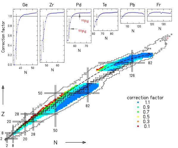
Figure 5: Bottom. Representation of the correction factor $h_{({\mathrm{N}}{\mathrm{Z}})}$ for secondary reaction on an isotopic chart for each residue measured in the reaction ²³⁸U+p at 1 A GeV [1, 2, 3]. Top. Isotopic distributions of $h_{({\mathrm{N}}{\mathrm{Z}})}$ for the elements Ge, Zr, Pd and Te, produced by fission and Pb and Fr, produced as evaporation residues. The dashed lines represent the residue corridor, calculated with the physical reaction code ABLA, imposing the sequential evaporation of higly excited heavy prefragments. The correction factor drops to very low values around the residue corridor: the steep slope of the “hook” shaped $h_{({\mathrm{N}}{\mathrm{Z}})}$ distribution determines the limit for the observation of primary reaction products and for the measurement of their isotopic cross sections. The correction for ¹⁰⁰Pd and ¹¹⁰Pd, indicated by arrows, can be compared to fig. (4).

The solution of the system (38) gives directly the value of the primary production cross-sections. As discussed in the references [8, 14, 15], a clear indication of the incidence of the secondary reactions on the experimental measurement can be deduced studying the variation of the correction factor

$$h_{({\mathrm{N}}{\mathrm{Z}})}=\sigma_{({\mathrm{N}}_{0}{\mathrm{Z}}_{0}\to{\mathrm{N}}{\mathrm{Z}})}\,/\,{\tilde{\sigma}}_{({\mathrm{N}}_{0}{\mathrm{Z}}_{0}\to{\mathrm{N}}{\mathrm{Z}})}$$

that we should apply to the apparent yields in order to obtain the primary cross-sections. In fig. (5) we mapped the values of $h_{({\mathrm{N}}{\mathrm{Z}})}$ for each measured isotope. The distribution shows mainly a plateau for a positive correction of around 5% to 7%: these values, originating from the first exponential term in Eq. (38) should compensate the effect of the losses. The homogeneity of the correction is then perturbed by the effect of the gain factor. In some cases, like the evaporation-residue production, this effect does not present complex features: generally, the secondary evaporation residues with low mass-loss in respect to the projectile should distribute on the same ridge of the primary production without showing a sensible deviation; as a consequence, the isobaric distributions should simply be scaled in height according to a constant factor and preserve the shape unchanged. This prescription could be followed as a rather good approximation in the case of heavy evaporation residues in reactions where no isotopes with high fissility are produced: the correction $h_{({\mathrm{N}}{\mathrm{Z}})}$ would reduce to a function of the mass-loss only. This was the approach applied in the analysis of the evaporation-residue production in the reaction of ¹⁹⁷Au+p at $800$ MeV [13], for the reaction ²⁰⁸Pb+p at $1$ GeV [8], and for the reaction ²⁰⁸Pb+d at $1$ GeV [15]. For these systems, and for the analysis of evaporation residues, this method would even have an advantage in respect to the application of the recursion (38): in fact, the assumption of an exclusive dependence of the correction $h_{({\mathrm{N}}{\mathrm{Z}})}$ on the mass-loss and the total cross-section of the intermediate fragment $\sigma_{({\mathrm{N}}_{i}{\mathrm{Z}}_{i})}$ allows to build a parameterisation based on the experimental data. On the other hand, the relation (38) suffers from the uncertainties introduced by the theoretical calculation of the intermediate-fragment cross-sections $\sigma_{({\mathrm{N}}_{i}{\mathrm{Z}}_{i}\to{\mathrm{N}}{\mathrm{Z}})}$. Indeed, for systems like ²³⁸U, dominated by a complicated competition between the fission and evaporation-residue channels, the correction factor $h_{({\mathrm{N}}{\mathrm{Z}})}$ can not be easily related to the mass-loss. Moreover, the distribution of the evaporation residues of ²³⁸U+p widens considerably around Pb: as a consequence the rain of secondary residues can not cover homogeneously the whole isobaric distribution and it will populate prevalently the neutron deficient side. As shown in fig. (5) this effect appears in the neutron-distribution of the correction factor for the element Pb and it induces a slight reduction of $h_{({\mathrm{N}}{\mathrm{Z}})}$ for low neutron numbers. This effect tends to disappear for heavier elements like Fr, characterized by an almost constant correction factor.

The use of a detailed description of the secondary reaction mechanisms becomes unavoidable when fission fragments should be treated: in this case $h_{({\mathrm{N}}{\mathrm{Z}})}$ largely changes as a function of the neutron number and the relation (38) can not be substituted by a parameterisation. As firstly formulated and demonstrated in the analysis of the fission residues in the reactions ²⁰⁸Pb+p at $1$ GeV [8], the correction factor is characterised by a “hook” shape and reduces steeply when it approaches the residues corridor. However, the steepness of the “hook” reflects also the steepness of the neutron-deficient side of the yield distribution. In fig. (5) an increased isotopic dependence of $h_{({\mathrm{N}}{\mathrm{Z}})}$ is shown for decreasing element numbers. The isotope ¹¹⁰Pd, whose formation mechanism has been illustrated above, is on the plateau of the $h_{({\mathrm{N}}{\mathrm{Z}})}$ function and the related cross-section should be corrected almost exclusively for the losses; on the contrary, ¹⁰⁰Pd is located on the slope of the correction factor. Other elements like Ge or Zr show corrections that even approach 100% for their lightest isotopes: of course, when the correction is too large, the rejection of these isotopes becomes necessary. Isotopes showing correction factors smaller than $0.5$ are omitted in the tabulation of cross sections in ref. [1]. The steep slope of the correction factor becomes a technical limit that excludes the possibility to extend the primary fission cross-section measurement to the neutron-deficient side.

We should still point out that, as shown in the definition (23), the gain factors include still another term: the transmission ratio for the secondary fragments ${\cal T}_{2}({\mathrm{N}}_{i}{\mathrm{Z}}_{i},{\mathrm{N}}{\mathrm{Z}})$ should be taken into account. As shown in fig. (6), the omission of the transmission ratio leads to an overestimation of the correction factor.

Figure 6: Study of the contribution of transmission in the calculation of the correction factor $h_{({\mathrm{N}}{\mathrm{Z}})}$. The transmission ratios are introduced as prescribed in Eq. (39,40,41)

The geometry of the spectrometer, as discussed in [16], has to be evaluated precisely in order to determine transmission values, which are deduced relating the experimentally observed velocities of the fragments, the acceptance of the spectrometer, and the beam velocity. The details of the calculation of these coefficients, used in this work, is described in [1]. In the case of intermediate fragments ${\mathrm{N}}_{i}{\mathrm{Z}}_{i}$, that are not detected, the transmission factor can not be measured directly. However, in this case we can still estimate the transmission factor because the velocities are known. In order to reduce the transmission ratios to only experimental values it is worth while applying the following approximations:

$${\cal T}_{2}^{\scriptstyle\mathrm{evr},\scriptstyle\mathrm{evr}}({\mathrm{N}}_{i}{\mathrm{Z}}_{i},{\mathrm{N}}{\mathrm{Z}})\, =\,\frac{t_{2}^{\scriptstyle\mathrm{evr},\scriptstyle\mathrm{evr}}({\mathrm{N}}_{i}{\mathrm{Z}}_{i},{\mathrm{N}}{\mathrm{Z}})}{t^{(}{\mathrm{N}}{\mathrm{Z}})}\,\approx\,\,1,$$ (39)

$${\cal T}_{2}^{\scriptstyle\mathrm{evr},\scriptstyle\mathrm{fis}}\,\,({\mathrm{N}}_{i}{\mathrm{Z}}_{i},{\mathrm{N}}{\mathrm{Z}})\, =\,\frac{t_{2}^{\scriptstyle\mathrm{evr},\scriptstyle\mathrm{fis}}\,\,({\mathrm{N}}_{i}{\mathrm{Z}}_{i},{\mathrm{N}}{\mathrm{Z}})}{t^{(}{\mathrm{N}}{\mathrm{Z}})}\,\approx\,\,1,$$ (40)

$${\cal T}_{2}^{\scriptstyle\mathrm{fis},\scriptstyle\mathrm{evr}}\,\,({\mathrm{N}}_{i}{\mathrm{Z}}_{i},{\mathrm{N}}{\mathrm{Z}})\, =\,\frac{t_{2}^{\scriptstyle\mathrm{fis},\scriptstyle\mathrm{evr}}\,\,({\mathrm{N}}_{i}{\mathrm{Z}}_{i},{\mathrm{N}}{\mathrm{Z}})}{t^{(}{\mathrm{N}}{\mathrm{Z}})}\,\approx\,\frac{t^{\scriptstyle\mathrm{fis}}({\mathrm{N}}_{i}{\mathrm{Z}}_{i})}{t^{\scriptstyle\mathrm{fis}}({\mathrm{N}}{\mathrm{Z}})}\,>1,$$ (41)

The relation (39) follows from simple considerations on the angular distribution of evaporation residues. In case of double reactions, the variance of the angular distribution in the laboratory is simply the sum of individual variances, which in turn are proportional to each individual mass loss, implying that the total variance is proportional to the total mass loss either for a secondary or primary reaction. This leads to $t_{2}^{\scriptstyle\mathrm{evr,evr}}({\mathrm{N}}_{i}{\mathrm{Z}}_{i},{\mathrm{N}}{\mathrm{Z}})\approx t^{(}{\mathrm{N}}{\mathrm{Z}})\,.$ when the primary production of NZ is mainly related to evaporation residues. We should observe that in some cases, when the primary production of NZ is mainly related to fission, and there is an additional contribution coming from secondary evaporation residues of primary evaporation residues, the ratio of Eq. (39) becomes greater than the unit. When fission is involved in the production of intermediate or secondary fragments, even though the same addition rule for the variance is applied, the variance for a process leading to evaporation residues is assumed to be much lower than in the case of fission, and it can be neglected. This leads to the relations  (40) and  (41). It should be observed that only the relation (41) is relevant in the calculation of the correction factor $h_{({\mathrm{N}}{\mathrm{Z}})}$. This derives from the observation that the variance of the angular distribution of a fission fragment ${\mathrm{N}}_{i}{\mathrm{Z}}_{i}$ is not strongly modified when the residue reacts again and produces a secondary residue by evaporation. We can then neglect the contribution of the secondary reaction to the variance and substitute the transmission coefficient $t_{2}^{\scriptstyle\mathrm{fis},\scriptstyle\mathrm{evr}}$, that can not be calculated on the base of experimental observables, with the transmission coefficient $t^{\scriptstyle\mathrm{fis}}$ of a fission fragment ${\mathrm{N}}_{i}{\mathrm{Z}}_{i}$; this leads to the the approximation $t_{2}^{\scriptstyle\mathrm{fis},\scriptstyle\mathrm{evr}}({\mathrm{N}}_{i}{\mathrm{Z}}_{i},{\mathrm{N}}{\mathrm{Z}})\approx t^{\scriptstyle\mathrm{fis}}({\mathrm{N}}_{i}{\mathrm{Z}}_{i})\,.$ Since the variance of the angular distribution for the fission fragment NZ is larger in respect to the lighter intermediate fission fragment ${\mathrm{N}}_{i}{\mathrm{Z}}_{i}$, the resulting term ${\cal T}_{2}^{\scriptstyle\mathrm{fis},\scriptstyle\mathrm{evr}}({\mathrm{N}}_{i}{\mathrm{Z}}_{i},{\mathrm{N}}{\mathrm{Z}})$ is larger than the unit.

6 Conclusion

This work presents a study on the formalism of multiple nuclear reactions induced in a target. A general model has been developed in order to simulate the isotopic yields of secondary reactions, distinguishing between fission and evaporation residues. The model described in this work became the base of the numerical code “SECONDARY”. The program has been tested to reproduce the secondary-reaction correction used in the analysis of the reactions ²⁰⁸Pb+p at $1$ A GeV [8] .The comparison resulted in good agreement with the previous calculations. The code SECONDARY, coupled with the reaction code ABLA [9, 10] and PROFI [11] has then been applied in the final step of the data-analysis presented in [1], aimed to determine the isotopic cross section of the reaction ²³⁸U+p at $1$ A GeV.

7 Acknowledgements

We are endebted to Karl-Heinz Schmidt for his expertise in reaction-model calculations, and for providing the codes BURST, ABLA and PROFI, necessary for the calculations presented in this work. We are grateful to Orlin Yordanov for his interest and fruitful discussions.

Appendix A Mathematical appendix

A.1 Extension of the description of the secondary reactions to the $n^{th}$ order.

The key relation to extend the description of the secondary reactions to the $n^{th}$ order is condensed in the following equality:

$$\sum_{i=0}^{n-1}\frac{1}{\underset{\scriptscriptstyle j=0\atop j\neq i}{\overset{\scriptscriptstyle n}{\prod}}(\sigma_{i}-\sigma_{j})}\quad=\quad-\frac{1}{\underset{\scriptscriptstyle j=0}{\overset{\scriptscriptstyle n-1}{\prod}}(\sigma_{n}-\sigma_{j})}.$$ (42)

Eq. (42) is a particular case, obtained imposing $k=n-1$ and $\lambda=\sigma_{n}$, of the following more general form:

$$\sum_{i=0}^{k}\frac{1}{(\sigma_{i}-\lambda)\underset{\scriptscriptstyle j=0\atop j\neq i}{\overset{\scriptscriptstyle k}{\prod}}(\sigma_{i}-\sigma_{j})}\quad=\quad-\frac{1}{\underset{\scriptscriptstyle j=0}{\overset{\scriptscriptstyle k}{\prod}}(\lambda-\sigma_{j})}.$$ (43)

For $k=0$ the equality is trivial, and it can also be checked for $k=1$. To prove Eq. (43) for any order, we should verify that the expression is recursive. If Eq. (43) is true at the order $k-1$, we can extend it to the order $k$ with the following passages:

$$\begin{split}&\displaystyle\sum_{i=0}^{k}\frac{1}{(\sigma_{i}-\lambda)\underset{\scriptscriptstyle j=0\atop j\neq i}{\overset{\scriptscriptstyle k}{\prod}}(\sigma_{i}-\sigma_{j})}\,=\\ &=\displaystyle\frac{1}{\sigma_{k}-\lambda}\Biggl{[}\frac{1}{\underset{\scriptscriptstyle j=0\atop j\neq i}{\overset{\scriptscriptstyle k-1}{\prod}}(\sigma_{k}-\sigma_{j})}+\sum_{i=0}^{k-1}\frac{\sigma_{k}-\lambda}{(\sigma_{i}-\lambda)\underset{\scriptscriptstyle j=0\atop j\neq i}{\overset{\scriptscriptstyle k}{\prod}}(\sigma_{i}-\sigma_{j})}\Biggr{]}\,=\\ &=\,\displaystyle\frac{1}{\sigma_{k}-\lambda}\Biggl{[}\frac{1}{\underset{\scriptscriptstyle j=0\atop j\neq i}{\overset{\scriptscriptstyle k-1}{\prod}}(\sigma_{k}-\sigma_{j})}+\sum_{i=0}^{k-1}\frac{\sigma_{k}-\lambda}{(\sigma_{i}-\sigma_{k})(\sigma_{i}-\lambda)}\frac{1}{\underset{\scriptscriptstyle j=0\atop j\neq i}{\overset{\scriptscriptstyle k-1}{\prod}}(\sigma_{i}-\sigma_{j})}\Biggr{]}\,=\\ &=\,\displaystyle\frac{1}{\sigma_{k}-\lambda}\Biggl{[}\frac{1}{\underset{\scriptscriptstyle j=0\atop j\neq i}{\overset{\scriptscriptstyle k-1}{\prod}}(\sigma_{k}-\sigma_{j})}+\sum_{i=0}^{k-1}\frac{1}{(\sigma_{i}-\sigma_{k})\underset{\scriptscriptstyle j=0\atop j\neq i}{\overset{\scriptscriptstyle k-1}{\prod}}(\sigma_{i}-\sigma_{j})}-\sum_{i=0}^{k-1}\frac{1}{(\sigma_{i}-\lambda)\underset{\scriptscriptstyle j=0\atop j\neq i}{\overset{\scriptscriptstyle k-1}{\prod}}(\sigma_{i}-\sigma_{j})}\Biggr{]}\end{split}$$

or, applying Eq. 43 to the last two terms in the brackets:

$$\begin{split}&=\,\frac{1}{\sigma_{k}-\lambda}\Biggl{[}\frac{1}{\underset{\scriptscriptstyle j=0\atop j\neq i}{\overset{\scriptscriptstyle k-1}{\prod}}(\sigma_{k}-\sigma_{j})}-\frac{1}{\underset{\scriptscriptstyle j=0\atop j\neq i}{\overset{\scriptscriptstyle k-1}{\prod}}(\sigma_{k}-\sigma_{j})}+\frac{1}{\underset{\scriptscriptstyle j=0}{\overset{\scriptscriptstyle k-1}{\prod}}(\lambda-\sigma_{j})}\Biggr{]}\,=\qquad\qquad\quad\\ &=\,-\frac{1}{\underset{\scriptscriptstyle j=0\atop j\neq i}{\overset{\scriptscriptstyle k}{\prod}}(\lambda-\sigma_{j})}.\end{split}$$ (44)

The probability for $n$ recursive reactions in the target, expressed in the Eq. (5) reduces to the Eq. (1,2,3) for $n$ equal to 0,1, and 2, respectivly. We can demonstrate that it is generally true if we obtain it recursively from ${\cal P}_{n-1}({\mathrm{N}}_{0}{\mathrm{Z}}_{0},{\mathrm{N}}_{1}{\mathrm{Z}}_{1},$ $\cdots$ $,{\mathrm{N}}_{n-1}{\mathrm{Z}}_{n-1},\chi)$ by applying Eq. (4). We reduce Eq. (5) to the order $n-1$ and we introduce it in Eq. (4):

$$\begin{split}&{\cal P}_{n}({\mathrm{N}}_{0}{\mathrm{Z}}_{0},{\mathrm{N}}_{1}{\mathrm{Z}}_{1},\cdots,{\mathrm{N}}_{n}{\mathrm{Z}}_{n},\chi)\,=\\ &\qquad\qquad=\,(-1)^{\displaystyle n-1}\,\sigma_{n-1\to n}\underset{\scriptscriptstyle i=1}{\overset{\scriptscriptstyle n-1}{\textstyle\prod}}\sigma_{(i-1\to i)}\,\sum_{i=0}^{n-1}\Biggl{[}e^{\displaystyle-\sigma_{n}\chi}\int_{0}^{\chi}\mathrm{d}\zeta\frac{e^{\displaystyle(\sigma_{n}-\sigma_{i})\zeta}}{\underset{\scriptscriptstyle j=0\atop j\neq i}{\overset{\scriptscriptstyle n-1}{\prod}}(\sigma_{i}-\sigma_{j})}\Biggr{]}\\ &\qquad\qquad=\,(-1)^{n-1}\,\underset{\scriptscriptstyle i=1}{\overset{\scriptscriptstyle n}{\textstyle\prod}}\sigma_{(i-1\to i)}\,\sum_{i=0}^{n-1}\frac{\,e^{\displaystyle-\sigma_{n}\chi}-e^{\displaystyle-\sigma_{i}\chi}}{\underset{\scriptscriptstyle j=0\atop j\neq i}{\overset{\scriptscriptstyle n}{\prod}}\displaystyle(\sigma_{i}-\sigma_{j})}.\qquad\qquad\quad\end{split}$$ (45)

If we apply the equality 42 we can prove that the Eq. (45) reduces to the form ( 5).

A.2 Extension of the approximated secondary reaction formalism to the $n^{th}$ order.

To prove that the Eq. (8) is a recursive extension of the Eq. (7) we should demonstrate that it could be derived from the order $n-1$, i.e. we have to solve the integral

$$\underset{\scriptscriptstyle i=1}{\overset{\scriptscriptstyle n}{\textstyle\prod}}\sigma_{(i-1\to i)}\,e^{\displaystyle-\sigma_{n}\chi}\int_{0}^{\chi}\frac{(\zeta)^{n-1}}{(n-1)!}\,e^{\displaystyle-\left(\frac{{\textstyle\sum_{j=0}^{n-1}}\,\sigma_{j}}{n}-\sigma_{n}\right)\zeta}\mathrm{d}\zeta.$$

If, before integrating, we expand the exponential to the $1^{\mathrm{st}}$ order in $\frac{1}{n}\sum_{j=0}^{n-1}\,\sigma_{j}\zeta-\sigma_{n}\zeta$, we reduce to the approximated form:

$$\begin{split}&\underset{\scriptscriptstyle i=1}{\overset{\scriptscriptstyle n}{\textstyle\prod}}\sigma_{(i-1\to i)}\,e^{\displaystyle-\sigma_{n}\chi}\biggl{[}\frac{\chi^{n}}{n!}+\biggl{(}\frac{{\textstyle\sum_{j=0}^{n-1}}\,\sigma_{j}}{n}-\sigma_{n}\biggr{)}\frac{\chi^{n+1}}{(n-1)!(n+1)}\biggr{]}\,=\\ &\quad\quad=\,\underset{\scriptscriptstyle i=1}{\overset{\scriptscriptstyle n}{\textstyle\prod}}\sigma_{(i-1\to i)}\,\frac{\chi^{n}}{n!}\,e^{\displaystyle-\sigma_{n}\chi}\,e^{\displaystyle-\biggl{(}\frac{{\textstyle\sum_{j=0}^{n-1}}\,\sigma_{j}}{n}-\sigma_{n}\biggr{)}\frac{n}{n+1}\,\chi},\end{split}$$

where the resulting expression is equal to Eq. (8).

References

• [1] M. Bernas, P. Armbruster, J. Benlliure, A. Boudard, E. Casarejos, S. Czajkowski, T. Enqvist, R. Legrain, S. Leray, B. Mustapha, P. Napolitani, J. Pereira-Conca, F. Rejmund, M.V. Ricciardi, K.-H. Schmidt, C. Stéphan, J. Taieb, L. Tassan-Got, C. Volant, Submitted to Nucl. Phys. A.
• [2] J. Taieb, K.-H. Schmidt, L. Tassan-Got, P. Armbruster, J. Benlliure, M. Bernas, A. Boudard, E. Casarejos, S. Czajkowski, T. Enqvist, R. Legrain, S. Leray, B. Mustapha, M. Pravikoff, F. Rejmund, C: Stéphan, C. Volant, W. Wlazlo submitted to Nucl. Phys. A, and thesis of J. Taieb, IPN-Orsay, 2000.
• [3] M.V. Ricciardi, K.-H. Schmidt, J. Benlliure, T. Enqvist, F. Rejmund, P. Armbruster, F. Ameil, M. Bernas, A. Boudard, S. Czajkowski, R. Legrain, S. Leray, B. Mustapha, M. Pravikoff, C. Stéphan, L. Tassan-Got, C. Volant XXXIX Int. Winter Meeting on Nucl. Phys., Bormio, Italy (2001), and thesis in progress of M.V. Ricciardi, GSI-Darmstadt.
• [4] H. Geissel, P. Armbruster, K.H. Behr, A. Brünle, K. Burkard, M. Chen, H. Folger, B. Franczak, H. Keller, O. Klepper, B. Langenbeck, F. Nickel, E. Pfeng, M. Pfützner, E. Roeckl, K. Rykaczewski, I. Schall, D. Schardt, C. Scheidenberger, K.-H. Schmidt, A. Schroter, T. Schwab, K. Sümmerer, M. Weber, G. Münzenberg, T. Brohm, H.-G. Clerc, M. Fauerbach, J.-J. Gaimard, A. Grewe, E. Hanelt, B. Knödler, M. Steiner, B. Voss, J. Weckenmann, C. Ziegler, A. Magel, H. Wollnik, J.P. Dufour, Y. Fujita, D.J. Vieira, B. Sherrill, Nucl. Instrum. Methods B 70, 286 (1992).
• [5] P. J. Karol, Phys. Rev. C 11, 1203 (1975).
• [6] T. Brohm, K.-H. Schmidt, Nucl. Phys. A 569, 821 (1994).
• [7] C.J. Benesh, B.C. Cook, J.P. Vary, Phys. Rev. C 40, 1198 (1989).
• [8] T. Enqvist, W. Wlazlo, P. Armbruster, J. Benlliure, M. Bernas, A. Boudard, S. Czajkowski, R. Legrain, S. Leray, B. Mustapha, M. Pravikoff, F. Rejmund, K.-H. Schmidt, C. Stéphan, J. Taieb, L. Tassan-Got, C. Volant, Nucl. Phys. A 686, 481 (2001).
• [9] J.-J. Gaimard, K.-H. Schmidt, Nucl. Phys. A 531, 709 (1991).
• [10] A.R. Junghans, M. de Jong, H.-G. Clerc, A.V. Ignatyuk, G.A. Kudyaev, K.-H. Schmidt, Nucl. Phys. A 629, 635 (1998).
• [11] J. Benlliure, A. Grewe, M. de Jong, K.-H. Schmidt, S. Zhdanov Nucl. Phys. A 628, 458 (1998).
• [12] K.-H. Schmidt, M.V. Ricciardi, A.S. Botvina, T. Enqvist, Nucl. Phys. A 710, 157 (2002).
• [13] F. Rejmund, B. Mustapha, P. Armbruster, J. Benlliure, M. Bernas, A. Boudard, J. P. Dufour, T. Enqvist, R. Legrain, S. Leray, K.-H. Schmidt, C. Stéphan, J. Taieb, L. Tassan-Got, C. Volant, Nucl. Phys. A 683, 540 (2001), and thesis of B. Mustapha, IPN-Orsay, 1999.
• [14] J. Benlliure, P. Armbruster, M. Bernas, A. Boudard, J. P. Dufour, T. Enqvist, R. Legrain, S. Leray, B. Mustapha, F. Rejmund, K.-H. Schmidt, C. Stéphan, L. Tassan-Got, C. Volant, Nucl. Phys. A 683, 513 (2001).
• [15] T. Enqvist, P. Armbruster, J. Benlliure, M. Bernas, A. Boudard, S. Czajkowski, R. Legrain, S. Leray, B. Mustapha, M. Pravikoff, F. Rejmund, K.-H. Schmidt, C. Stéphan, J. Taieb, L. Tassan-Got, F. Vivès, C. Volant, W. Wlazlo Nucl. Phys. A 703, 435 (2002)
• [16] J. Benlliure, J. Pereira-Conca, K.-H. Schmidt, Nucl. Instrum. Methods. A 478, 493 (2002).