Precise laser spectroscopy of the antiprotonic helium atom and CPT test on antiproton mass and charge

Abstract

We have measured twelve transition frequencies of the antiprotonic helium atom ($\bar{p}$He⁺) with precisions of 0.1–0.2 ppm using a laser spectroscopic method. The agreement between the experiment and theories was so good that we can put a limit on the proton-antiproton mass (or charge) difference. The new limit is expected to be much smaller than the already published value, 60 ppb ($6\times 10^{-8}$).

1 Introduction

The antiprotonic helium atom ($\bar{p}$He⁺) is a three-body system consisting of an antiproton, an electron, and a helium nucleus. Some states (quantum numbers; $n$, $l$ $\sim$ 38) of this exotic atom are known to live anomalously long (lifetime $\sim$ 3 $\mu$s) for a system including an antiproton. Since its discovery in 1991 [1, 2], the nature of this antiprotonic atom has been studied extensively, and precise measurements of its enegy levels have been carried out using a laser spectroscopic method.

In the last few years we have performed sub-ppm laser spectroscopy on many transitions of the antiprotonic atom at CERN AD (Antiproton Decelerator) [3]. We have done a CPT test on proton-antiproton mass and charge differences by comparing the experiment with theories, as the theories use the known proton mass value for the antiproton mass.

2 Experimental Setup

Our current experimental scheme is in principle the same as the one described in Refs. [3, 4]. A major improvement is that we started to use a new radiofrequency quadrupole decelerator (RFQD) [5]. The apparatus can decelerate antiprotons from 5.3 MeV to below 100 keV by a RFQ electric field. Previously, we had to use a gas target dense enough to stop 5.3 MeV antiprotons (atomic density $\rho\sim 10^{21}$ cm^-3), but such a high density can shift the resonant frequency significantly. By using the RFQD, antiprotons can be stopped in a far lower density target ($\rho=10^{17}$–$10^{18}$ cm^-3), thus we can directly measure the transition frequencies at “zero-density”, instead of taking several scans at different target densities and making an extrapolation.

3 Analysis

3.1 Transition frequency

The analysis method for the transition frequencies is also concisely described in the Refs. [3, 4]. Here we summarize the three procedures used for the deduction of the frequencies.

• Fitting the frequency profiles of the resonances
  Each resonance profile was fitted with a sum of two identical-shaped Voigt functions separated by the theoretical hyperfine splitting [6, 7]. The uncertainty of the fitting is $\Delta\nu=$ 20–60 MHz, which mainly comes from statistical fluctuations, instability of the laser power, and irregular frequency distributions of the laser pulse.

• Absolute frequency calibration
  Our wavelength meter is absolutely calibrated against molecular ro-vibrational lines of iodine [8, 9] or tellurium, or atomic lines of neon or argon by optogalvanic spectroscopy. The accuracy of the calibration is 20–50 MHz.

• Density extrapolaration
  For high density (non-RFQD) scans, transition frequencies at zero-density were obtained by linear extrapolation of the several central frequencies at different densities. Due to the limited accuracy of the temperature and pressure measurement, this procedure causes 20–50 MHz of uncertainty.

By taking into account all of the above, the overall precision $\Delta\nu/\nu$ was 0.1–0.2 ppm.

3.2 CPT test

The agreement between the experiment and theories enables us to put a limit on the proton-antiproton mass (or charge) difference, which is equal to zero if the CPT theorem holds. Here we describe how we could obtain the CPT limit from the experimental results.

The charge-to-mass ratio of antiproton $Q_{\bar{p}}/M_{\bar{p}}$ has been measured to a high precision of $9\times 10^{-11}$ by a Penning trap experiment [10]. Our experiment measures transition frequencies, which are differences of energy levels. The frequency of an antiprotonic transition should depend on the antiproton mass and the charge. If we assume a hydrogen-like system, this dependence can be written as

$$\hbar\nu=\Delta E\propto M_{\bar{p}}Q_{\bar{p}}^{2}.$$ (1)

However, the actual dependence is different from the above, because the system consists of three particles and the antiproton is quite heavy. Instead, we can write the realistic dependence by introducing a parameter $f$, which depends on the transition:

$$\Delta E\propto M_{\bar{p}}Q_{\bar{p}}^{f-1}=({Q_{\bar{p}}}/{M_{\bar{p}}})^{-1}Q_{\bar{p}}^{f}=({Q_{\bar{p}}}/{M_{\bar{p}}})^{f-1}M_{\bar{p}}^{f}.$$ (2)

If we fix the well-known charge-to-mass ratio, $\Delta E$ is simply proportional to $Q_{\bar{p}}^{f}$ and $M_{\bar{p}}^{f}$. The parameter $f=$ 2–6 was theoretically evaluated by Kino [11] by calculating the shift of the transition frequency when the input proton mass value is changed slightly.

Then, the CPT limit parameter $\delta$ can be obtained by comparing the experimental and theoretical values:

$$\delta=\frac{Q_{p}+Q_{\bar{p}}}{Q_{p}}=\frac{M_{p}-M_{\bar{p}}}{M_{p}}=\frac{1}{f}\frac{\nu_{th}-\nu_{exp}}{\nu_{exp}},$$ (3)

since the theories use the precisely-known proton mass as the antiproton mass in the calculations. The limits of all the twelve transitions were averaged to obtain the final result.

4 Results

Fig. 1 shows the comparison of the experimental and the theoretical transition frequencies published in 2001 [3]. In this figure, the experimental values are centered on the dotted lines and their precisions $\Delta\nu_{exp}/\nu_{exp}$ are shown as error bars. Two independent calculations by Korobov [12] and Kino [13] are compared with our results. Although not shown in this figure, eight more states of $\bar{p}^{4}$He⁺ and $\bar{p}^{3}$He⁺ measured in 2001–2002 are in analysis.

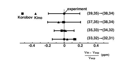
Figure 1: Precise comparison of the experimental and the theoretical transition frequencies of $\bar{p}$⁴He⁺ [3].

Table 1 is the summary of our progress. From the measurements in 2000, we obtained a CPT limit of 60 ppb with a confidence level of 90% [3]. Since then, many transitions including those of $\bar{p}^{3}$He⁺ were measured, and the RFQD contributed to an efficient data-taking. As a result, the CPT limit is, according to our preliminary analysis so far, greatly improved by a factor 3 or better. The final result of the analysis will be presented in [15].

Table 1: Summary of the progress of our measurement at AD.

Year	2000	2001–2002
Precision of each frequency	0.2 ppm	0.1 – 0.2 ppm
Measured transitions	4	12
$\bar{p}$He isotope	$\bar{p}$4He only	$\bar{p}$3He, $\bar{p}$4He
RFQD	Not used	Used
CPT limit $|\delta|$ (90% C.L.)	60 ppb	$<$ 20 ppb (preliminary)
Publication	[3], referred by [14]	[15](to be published)

We are grateful to CERN PS division for their help, V.I. Korobov, D.D. Bakalov and Y. Kino for useful discussions. This work was supported by the Grant-in-Aid for Creative Basic Research (Grant No. 10NP0101) of Monbukagakusho of Japan, and the Hungarian Scientific Research Fund (Grant Nos. OTKA T033079 and TeT-Jap-4/00).

References

- [1] M. Iwasaki et al., Phys. Rev. Lett. 67 (1991) 1246.
- [2] T. Yamazaki et al., Nature (London) 361 (1993) 238.
- [3] M. Hori et al., Phys. Rev. Lett. 87 (2001) 093401.
- [4] M. Hori et al., Nucl. Instr. and Meth. A (to be publshed).
- [5] W. Pirkl et al. (unpublished).
- [6] E. Widmann et al., Phys. Lett. B 404, (1997) 15.
- [7] D.D. Bakalov and V.I. Korobov, Phys. Rev. A 57, (1998) 1662.
- [8] S.C. Xu et al. J. Mol. Spectrosc. 201, (2000) 256.
- [9] B. Bordermann et al. Eur. Phys. J. D 11, (2000) 213.
- [10] G. Gabrielse et al., Phys. Rev. Lett. 82, (1999) 3198.
- [11] Y. Kino (private communication).
- [12] V.I. Korobov and D.D. Bakalov, Phys. Rev. Lett. 79, (1997) 3379; (private communication).
- [13] Y. Kino, M. Kamimura, and H. Kudo, Hyperfine Interactions 119, (1999) 201; (private communication).
- [14] Particle Data Group, K. Hagiwara et al. Phys. Rev. D 66, (2002) 010001.
- [15] M. Hori et al. (unpublished).