Abstract

The ensemble of experimental data on the 2830 nuclides which have been observed since the beginning of Nuclear Physics are being evaluated, according to their nature, by different methods and by different groups. The two “horizontal” evaluations in which I am involved: the Atomic Mass Evaluation Ame and the Nubase evaluation belong to the class of “static” nuclear data. In this lecture I will explain and discuss in detail the philosophy, the strategies and the procedures used in the evaluation of atomic masses.

Résumé L’évaluation des masses atomiques - Les données expérimentales sur les 2830 nucléides observés depuis les débuts de la Physique Nucléaire sont évaluées, suivant leur nature, par différentes méthodes et par différents groupes. Les deux évaluations “horizontales” dans les- quelles je suis impliqué : l’Évaluation des Masses Atomiques Ame et l’évaluation Nubase appartiennent à la classe des données nucléaires “statiques”. Dans ce cours je vais expliquer et discuter de manière approfondie la philosophie, les stratégies et les procédures utilisées dans l’évaluation des masses atomiques.

PACS.   21.10.Dr ; 21.10.Hw ; 21.10.Tg ; 23.40.-s ; 23.50.+z ; 23.60.+e
Keywords:   Binding energies - atomic masses - horizontal evaluation - nuclear data - least-squares - predictions of unknown masses

1 Introduction

Nuclear Physics started a little bit more than 100 years ago with the discoveries of natural radioactivity by Henri Becquerel and Pierre and Marie Curie; and of the atomic nucleus in 1911 by Ernest Rutherford with his assistants Ernest Marsden and Hans Geiger. First, it was a science of curiosity exhibiting phenomena unusual for that time. It is not until the late thirties, well after the discovery of artificial radioactivity by Frédéric and Irène Joliot-Curie, that the research in that domain tended to accelerate drastically and that Nuclear Physics became more and more a quantitative science.

Since then, scientists have accumulated a huge amount of data on a large number of nuclides. Today there are some 2830 variations on the combination of protons and neutrons that have been observed. Although this number seems large, specially compared to the 6 000 to 7 000 that are predicted to exist, one should be aware that the numbers of protons and neutrons constituting a nuclide are not really independent. Their special correlation form a relatively narrow band around a line called the bottom of the valley of stability. In Fig. 1 this is illustrated for the known masses (colored ones) across the chart of nuclides. In other words, nuclear data put almost no constraint in isospin on nuclear models. From there follows the tendency of nuclear physicists to study nuclides at some distance from that line, which are called exotic nuclides.

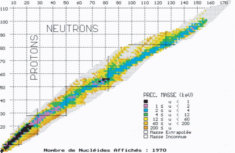
Figure 1: Chart of nuclides for the precision on masses. Only the known masses are colored, exhibiting crudely the narrowness of the valley of our knowledge in this immense landscape. Would these 1970 known masses been scattered around in the ($N,Z$) plane, our understanding of the nucleus would have been completely changed.

Sometimes remeasurement of the same physical quantity improved a previous result; sometimes it entered in conflict with it. The interest of the physicist has also evolved with time: the quantities considered varied importantly, scanning all sort of data from cross sections to masses, from half-lives to magnetic moments, from radii to superdeformed bands.

Thus, we are left nowadays with an enormous quantity of information on the atomic nucleus that need to be sorted, treated in a homogeneous way, while keeping traceability of the conditions under which they were obtained. When necessary, different data yielding values for the same physical quantity need to be compared, combined or averaged to derive an adopted value. Such values will be used in domains of physics that can be very far from nuclear physics, like half-lives in geo-chronology, cross-sections in proton-therapy, or masses in the determination of the $\alpha$ fine structure constant.

There are two classes of nuclear data: one class is for data related to nuclides at rest (or almost at rest); and the other class is for those related to nuclidic dynamics. In the first class, one finds ground-state and level properties, whereas the second encompasses reaction properties and mechanisms.

Nuclear ground-state masses and radii; magnetic moments; thermal neutron capture cross-sections; half-lives, spins and parities of excited and ground-state levels; the relative position (excitation energies) of these levels; their decay modes and the relative intensities of these decays; the transition probabilities from one level to another and the level width; the deformations; all fall in the category of what could be called the “static” nuclear properties.

Total and differential (in energy and in angle) reaction cross-sections; reaction mechanisms; and spectroscopic factors could be grouped in the class of “dynamic” nuclear properties.

Certainly, one single experiment, for example a nuclear reaction study, can yield data for both ‘static’ and ‘dynamic’ properties.

It is out of the scope of the present lecture to cover all aspects of nuclear properties and nuclear data. The fine structure of “static” nuclear data will be shortly described and the authors of the various evaluations presented. Then I will center this lecture on the two “horizontal” evaluations in which I am involved: the atomic mass evaluation Ame and the Nubase evaluation, both being strongly related, particularly when considering isomers.

2 “Static” nuclear data

2.1 The Nsdd: data for nuclear structure

The amount of data to be considered for nuclear structure is huge. They are represented schematically in Fig. 2 for each nuclide as one column containing all levels from the ground-state at the bottom of that column to the highest known excited state. All the known properties for each of the levels are included.

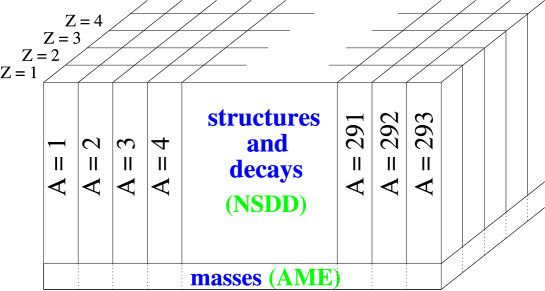
Figure 2: Schematic representation of all the available “static” nuclear data (structure, decay, mass, radius, moments,…). Each nuclide is represented as a building with its ground-state at the ground floor. The mass evaluation is represented on the ground floor, across all buildings. It includes also data for upper levels if they represent an energy relation to another nuclide, like a foot-bridge between two buildings that will allow to derive the level difference between their ground floors.

Very early, it was found convenient to organize their evaluation in a network, splitting these data according to the mass of the nuclides, the $A$-chains. Such a division makes sense, since most of the decay relations among nuclides are $\beta$-decays where $A$ is conserved. This is, of course, less true for heavier nuclides where $\alpha$-decay is the dominant decay-mode connecting an $A$-nuclide to an $A-4$ daughter. This structure is the one adopted by the Nuclear Structure and Decay Data network (the Nsdd) organized internationally under the auspices of the Iaea in Vienna. An $A$-chain or a group of successive $A$-chains is put under the responsibility of one member of the network. His or her evaluation is refereed by another member of the network before publication in the journal ‘Nuclear Data Sheets’ (or in the ‘Nuclear Physics’ journal for $A~{}\leq~{}44$). At the same time the computer files of the evaluation (the Ensdf: ‘Evaluated Nuclear Structure Data Files’) are made available at the Nndc-Brookhaven [1]. In this evaluation network, most of the “static” nuclear data are being considered.

The Nsdd evaluation for each nuclide is not dependent, at first order, on the properties of a neighboring nuclide, except when there is a decay relation with that neighbor. Such evaluation, conducted nuclide by nuclide, is called a ‘vertical’ evaluation.

2.2 The atomic mass evaluation Ame

However, the evaluation of data for energy relations between nuclides is more complex due to numerous links that overdetermine the system and exhibit sometimes inconsistencies among data. This ensemble of energy relations is taken into account in the ‘horizontal’ structure of the Atomic Mass Evaluation Ame [3, 4]. By ‘horizontal’ one means that a unique nuclear property is being considered across the whole chart of nuclides, here the ground-state masses. Only such a structure allows to encompass all types of connections among nuclides, whether derived from $\beta$-decays, $\alpha$-decays, thermal neutron-capture, reaction energies, or mass-spectrometry where any nuclide, e.g. ²⁰⁰Hg can be connected to a molecule like ¹²C¹³C³⁵Cl₅ or, in a Penning trap mass spectrometer, to ²⁰⁸Pb.

The Ame, the main subject of this lecture, will be developed below, in Section  3.

2.3 The isomers in the Ame and the emergence of Nubase

At the interface between the Nsdd and the Ame, one is faced with the problem of identifying - in some difficult cases - which state is the ground-state. The isomer matter is a continuous subject of worry in the Ame, since a mistreatment can have important consequences on the ground-state masses. Where isomers occur, one has to be careful to check which one is involved in reported experimental data, such as $\alpha$- and $\beta$-decay energies. Cases have occurred where authors were not (yet) aware of isomeric complications. The matter of isomerism became even more important, when mass spectrometric methods were developed to measure masses of exotic atoms far from $\beta$-stability and therefore having small half-lives. The resolution in the spectrometers is limited, and often insufficient to separate isomers. Then, one so obtains an average mass for the isomeric pair. A mass of the ground-state, our primary purpose, can then only be derived if one has information on the excitation energy and on the production rates of the isomers. And in cases where e.g. the excitation energy was not known, it may be estimated, see below.

When an isomer decays by an internal transition, there is no ambiguity and the assignment as well as the excitation energy is given by the Nsdd evaluators. However, when a connection to the ground-state cannot be obtained, most often a decay energy to (and sometimes from) a different nuclide can be measured (generally with less precision). In the latter case one enters the domain of the Ame, where combination of the energy relations of the two long-lived levels to their daughters (or to their parents) with the masses of the latter, allows to derive the masses of both states, thus an excitation energy (and, in general, an ordering).

Up to the 1993 mass table, the Ame was not concerned with all known cases of isomerism, but only in those that were relevant to the determination of the ground-state masses. In 1992 it was decided, after discussion with the Nsdd evaluators, to include all isomers for which the excitation energy “is not derived from $\gamma$-transition energy measurements ($\gamma$-rays and conversion electron transitions), and also those for which the precision in $\gamma$-transitions is not decidedly better than that of particle decay or reaction energies leading to them” [2].

However, differences in isomer assignment between the Nsdd and the Ame evaluations cannot be all removed at once, since the renewal of all $A$-chains in Nsdd can take several years. In the meantime also, new experiments can yield information that could change some assignments. Here a ‘horizontal’ evaluation should help.

The isomer matter was one of the main reasons for setting up in 1993 the Nubase collaboration leading to a thorough examination and evaluation of those ground-state and isomeric properties that can help in identifying which state is the ground-state and which states are involved in a mass measurement [5]. Nubase appears thus as a ‘horizontal’ database for several nuclear properties: masses, excitation energies of isomers, half-lives, spins and parities, decay modes and their intensities. Applications extend from the Ame to nuclear reactors, waste management, astrophysical nucleo-synthesis, and to preparation of nuclear physics experiments.

Setting up Nubase allowed in several cases to predict the existence of an unknown ground-state from trends of isomers in neighboring nuclides, whereas only one long-lived state was reported. A typical example is ¹⁶¹Re, for which Nubase’97 [6] predicted a (${1/2}^{+}\#$) proton emitting state below an observed 14 ms $\alpha$-decaying high-spin state. (Everywhere in Ame and Nubase the symbol # is used to flag values estimated from trends in systematics.) Since then, the 370 $\mu$s, ${1/2}^{+}$, proton emitting state was reported with a mass 124 keV below the 14 ms state. For the latter a spin ${11/2}^{-}$ was also assigned [7]. Similarly, the ${11/2}^{-}$ bandhead level discovered in ¹²⁷Pr [8] is almost certainly an excited isomer. We estimate for this isomer, from systematical trends, an excitation energy of 600(200)# keV and a half-life of approximatively 50# ms.

In some cases the value determined by the Ame for the isomeric excitation energy allows no decision as to which of the two isomers is the ground-state. This is particularly the case when the uncertainty on the excitation energy is large compared to that energy, e.g.: $E^{m}(^{82}$As)$=250\pm 200$ keV; $E^{m}(^{134}$Sb)$=80\pm 110$ keV; $E^{m}(^{154}$Pm)$=120\pm 120$ keV.

Three main cases may occur. In the first case, there is no indication from the trends in $J^{\pi}$ systematics of neighboring nuclides with same parities in $N$ and $Z$, and no preference for ground-state or excited state can be derived from nuclear structure data. Then the adopted ordering, as a general rule, is such that the obtained value for $E^{m}$ is positive. In the three examples above, ⁸²As will then have its (5^-) state located at 250$\pm$200 keV above the (1⁺); in ¹³⁴Sb the (7^-) will be 80$\pm$110 keV above (0^-); and ¹⁵⁴Pm’s spin (3,4) isomer 120$\pm$120 keV above the (0,1) ground-state. In the second case, one level could be preferred as ground-state from consideration of the trends of systematics in $J^{\pi}$. Then, the Nubase evaluators accept the ordering given by these trends, even if it may yield a (slightly) negative value for the excitation energy, like in ¹⁰⁸Rh (high spin state at $-60\pm$110 keV). Such trends in systematics are still more useful for odd-$A$ nuclides, for which isomeric excitation energies of isotopes (if $N$ is even) or, similarly, isotones follow usually a systematic course. This allows to derive estimates both for the relative position and for the excitation energies where they are not known. Finally, there are cases where data exist on the order of the isomers, e.g. if one of them is known to decay into the other one, or if the Gallagher-Moszkowski rule [9] for relative positions of combinations points strongly to one of the two as being the ground-state. Then the negative part, if any, of the distribution of probability has to be rejected (Fig. 3). Value and error are then calculated from the moments of the positive part of the distribution.

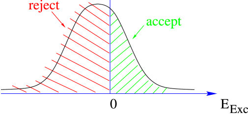
Figure 3: Truncated distribution of probability when there is a strong indication about ordering of ground-state and isomer.

2.4 Other ‘horizontal’ evaluations

There might be other reasons for ‘horizontal’ evaluations. The splitting of data among a large number of evaluators - like in the Nsdd network described above - does not always allow having a completely consistent treatment of a given nuclear property through the chart of nuclides. In addition, some quantities may fall at the border of the main interest of such a network. This is the reason why a few ‘horizontal’ compilations or evaluations have been conducted for the benefit of the whole community. For example, one can quote the work of Otten [10] for isotope shift and hyperfine structure of spectral lines and the deduced radii, spins and moments of nuclides in their ground-state and long-lived isomeric states. An evaluation of isotope shifts has been published also by Aufmuth and coworkers [11], and Raghavan [12] gave a table of nuclear moments, updated recently by Stone [13]. More recent tables for nuclidic radii were published by Angeli [14] in 1991 and by Nadjakov et al [15] in 1994. Two other ‘horizontal’ evaluations are worth mentioning. One is the evaluation of isotopic abundances, by Holden [16]. The second one is the evaluation of Raman and coworkers [17] for the energy $E_{2^{+}}$ and the reduced electric quadrupole transition probability $B(E2)$ of the first excited $2^{+}$ state in even-even nuclides.

3 The evaluation of atomic masses (Ame)

The atomic mass evaluation is particular when compared to the other evaluations of data reviewed above, in that there are almost no absolute determinations of masses. All mass determinations are relative measurements. Each experimental datum sets a relation in energy or mass among two (in a few cases, more) nuclides. It can be therefore represented by one link among these two nuclides. The ensemble of these links generates a highly entangled network. This is the reason why, as I mentioned earlier (cf. Section 2.2), a ‘horizontal’ evaluation is essential.

I will not enter in details in the different types of mass experiments, since there are other lectures devoted to this subject [18]. Nevertheless, I need to sketch the various classes of mass measurements to outline how they enter the evaluation of masses and how they interfere with each other.

Generally a mass measurement can be obtained by establishing an energy relation between the mass we want to determine and a well known nuclidic mass. This energy relation is then expressed in electron-volts (eV). Mass measurements can also be obtained as an inertial mass from its movement characteristics in an electro-magnetic field. The mass, thus derived from a ratio of masses, is then expressed in ‘unified atomic mass’ (u) (cf. Section 3.1.3), or its sub-unit, $\mu$u. Two units are thus used in the present work.

The mass unit is defined, since 1960, by 1 u $={\cal M}(^{12}$C$)/12$, one twelfth of the mass of one free atom of Carbon-12 in its atomic and nuclear ground-states. Before 1960, as Wapstra once told me, two mass units were defined: the physical one ¹⁶O$/16$, and the chemical one which considered one sixteenth of the average mass of a standard mixture of the three stable isotopes of oxygen. Physicists could not convince the chemists to drop their unit; “The change would mean millions of dollars in the sale of all chemical substances”, said the chemists, which is indeed true! Joseph H.E. Mattauch, the American chemist Truman P. Kohman and Aaldert H. Wapstra [19] then calculated that, if ¹²C$/12$ was chosen, the change would be ten times smaller for chemists, and in the opposite direction …That lead to unification; ‘u’ stands therefore, officially, for ‘unified mass unit’! Let us mention to be complete that the chemical mass spectrometry community (e.g. bio-chemistry, polymer chemistry) widely use the dalton (symbol Da, named after John Dalton [20]), which allows to express the number of nucleons in a molecule. It is thus not strictly the same as ‘u’.

The energy unit is the electronvolt. Until recently, the relative precision of $M-A$ expressed in keV was, for several nuclides, less good than the same quantity expressed in mass units. The choice of the volt for the energy unit (the electronvolt) is not evident. One might expect use of the international volt V, but one can also choose the standard volt V₉₀ as maintained in national laboratories for standards and defined by adopting an exact value for the constant ($2e/h$) in the relation between frequency and voltage in the Josephson effect. In the 1999 table of standards [21]: $2e/h=483597.9$ (exact) GHz/V₉₀. An analysis by Cohen and Wapstra [22] showed that all precision measurements of reaction and decay energies were calibrated in such a way that they can be more accurately expressed in V₉₀. Also, the precision of the conversion factor between mass units and standard volts V₉₀ is more accurate than that between it and international volts V:

$$1\,{\rm u} = 931\,494.009\,0\pm 0.007\,1\phantom{0}{\rm keV}_{90}$$

$$1\,{\rm u} = 931\,494.013\,\phantom{0}\pm 0.037\,\phantom{0}\phantom{0}{\rm keV}$$

The reader will find more information on the energy unit, and also some historical facts about the electronvolt, in the Ame2003 [3], page 134.

3.1 The experimental data

In this section we shall examine the various types of experimental information on masses and see how they enter the Ame.

3.1.1 Reaction energies

The energy absorbed in a nuclear reaction is directly derived from the Einstein’s relation $E=mc^{2}$. In a reaction A(a,b)B requiring an energy $Q_{r}$ to occur, the energy balance writes:

$$Q_{r}={\cal M}_{\rm A}+{\cal M}_{\rm a}-{\cal M}_{\rm b}-{\cal M}_{\rm B}$$ (1)

This reaction is often endothermic, that is $Q_{r}$ is negative, requiring input of energy to occur. Other nuclear reactions may release energy. This is the case, for example, for thermal neutron-capture reactions (n,$\gamma$) where the (quasi)-null energetic neutron is absorbed and populates levels in the continuum of nuclide ‘B’ at an excitation energy exactly equal to $Q_{r}$. With the exception of some reactions between very light nuclides, the the masses of the projectile ‘a’ and of the ejectile ‘b’ are known with a much higher accuracy than those of the target ‘A’, and of course the residual nuclide ‘B’. Therefore Eq. 1 reduces to a linear combination of the masses of two nuclides:

$${\cal M}_{\rm A}-{\cal M}_{\rm B}=q\pm dq$$ (2)

where $q=Q_{r}-{\cal M}_{\rm a}+{\cal M}_{\rm b}$.

A nuclear reaction usually deals with stable or very-long-lived target ‘A’ and projectile ‘a’, allowing only to determine the mass of a residual nuclide ‘B’ close to stability. Nowadays with the availability of radioactive beams, interest in reaction energy experiments is being revived.

It is worth mentioning in this category the very high accuracies attainable with (n,$\gamma$) and (p,$\gamma$) reactions. They play a key-rôle in providing many of the most accurate mass differences, and help thus building and strengthening the “backbone” of masses along the valley of $\beta$-stability, and determine neutron separation energies with high precision.

Also very accurate are the self-calibrated reaction energy measurements using spectrometers. When measuring the difference in energy between the spectral lines corresponding to reactions A(a,b)B and C(a,b)D with the same spectrometer settings [24] one can reach accuracies better than 100 eV. Here the measurement can be represented by a linear combination of the masses of four nuclides:

$$\delta Q_{r}={\cal M}_{\rm A}-{\cal M}_{\rm B}-{\cal M}_{\rm C}+{\cal M}_{\rm D}$$ (3)

The most precise reaction energy is the one that determined the mass of the neutron from the neutron-capture energy of ¹H at the Ill [25]. The ¹H(n,$\gamma$)²H established a relation between the masses of the neutron, of ¹H and of the deuteron with the incredible precision of 0.4 eV.

3.1.2 Disintegration energies

Disintegration can be considered as a particular case of reaction, where there is no incident particle. Of course, here the energies $Q_{\beta}$, $Q_{\alpha}$ or $Q_{p}$ are almost always positive, i.e. these particular reactions are exothermic. For the A($\beta^{-}$)B, A($\alpha$)B or A(p)B disintegrations, one can write respectively:

$$Q_{\beta^{-}} = {\cal M}_{\rm A}-{\cal M}_{\rm B}$$ (4)

$$Q_{\alpha}\,\, = {\cal M}_{\rm A}-{\cal M}_{\rm B}-{\cal M}_{\alpha}$$ (5)

$$Q_{p}\,\, = {\cal M}_{\rm A}-{\cal M}_{\rm B}-{\cal M}_{\rm p}$$ (6)

These measurements are very important because they allow deriving masses of unstable or very unstable nuclides.

This is more specially the case for the proton decay of nuclides at the drip-line, in the medium-$A$ region [26]. They allow a very useful extension of the systematics of proton binding energies. But in addition they give in several cases information on excitation energies of isomers. This development is one more reason why we have to give more attention to relative positions of isomers than was necessary in earlier evaluations.

$\alpha$-decays have permitted to determine the masses of the heavy nuclides. Moreover, the time coincidence of $\alpha$ lines in a decaying chain allows very clear identification of the heaviest ones. Quite often, and more particularly for even-even nuclides, the measured $\alpha$-decay energies yield quite precise mass differences between parent and daughter nuclide.

3.1.3 Mass Spectrometry

Mass-spectrometric determination of atomic masses are often called ‘direct’ mass measurements because they are supposed to determine not an energy relation between two nuclides, but directly the mass of the desired one. In principle this is true, but only to the level of accuracy of the parameter of the spectrometer that is the least well known, which is usually the magnetic field in which the ions move. It follows that the accuracy in such absolute direct mass determination is very poor.

This is why, in all precise mass measurements, the mass of an unknown nuclide is always compared, in the same magnetic field, to that of a reference nuclide. Thus, one determines a ratio of masses, where the value of the magnetic field cancels, leading to a much more precise mass determination. As far as the Ame is concerned, here again we have a mass relation between two nuclides.

One can distinguish three sub-classes in the class of mass measurement by mass-spectrometry (see also [18]):

1. Classical mass-spectrometry, where the electromagnetic deflection plays the key-rôle. More exactly, the two beams corresponding to the ion of the investigated nuclide and to that of the reference are forced to follow the same path in the magnetic field. The ratio of the voltages of some electrostatic devices that make this condition true determines the ratio of masses. These voltages are determined either from the values of resistors in a bridge [27] or directly from a precision voltmeter [28].

2. Time-of-Flight spectrometry, where one measures simultaneously the momentum of an ion (from its magnetic rigidity $B\rho$) and its velocity (from the time of flight along a path of well-determined length) [29]. Calibration in this type of experiment requires a large set of reference masses, so that the Ame cannot establish a simple relation between two nuclides. Nevertheless, the calibration function thus determined, together with its contribution to the error is generally well accounted for. The chance is small that recalibration might be necessary. In case it appears to be so in some future, one could consider a global re-centering of the published values. It is interesting to note that Time-of-Flight spectrometers can be also set-up in cyclotrons [30] or in storage rings [31].

3. Cyclotron Frequency, when measured in a homogeneous magnetic field, yields mass value of very high precision due to the fact that frequency is the physical quantity that can be measured with the highest accuracy with the present technology. Three types of spectrometers follow this principle:

   • the Radio-Frequency Mass Spectrometer (Fig. 4) invented by L.G. Smith [32] where the measurement is obtained in-flight, as a transmission signal, in only one turn;

     

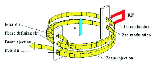
     Figure 4: Principle of the Radio-Frequency Mass Spectrometer. Ions make two turns following a helicoidal path in a homogeneous field $\vec{B}$. Two RF excitations are applied at one turn interval. Only ions for which the two excitations are in opposite phase (and then cancel) will exit the spectrometer and be detected. Typical diameter of the helix is 0.5-1 meter. This scheme is from the Mistral Web site: http://csnwww.in2p3.fr/groupes/massatom/.

   • the Penning Trap Spectrometer (Fig. 5) where the ions are stored for 0.1–2 seconds to interact with a radio-frequency excitation signal [33]; and

     

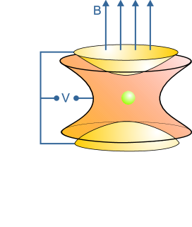
     Figure 5: Principle of the Penning Trap Spectrometer. Ions follow a cyclotron motion in the horizontal plane due to $\vec{B}$ and cannot escape axially due to repulsion by the end-cup electrodes. The ring electrode is split to allow RF excitation. Typical inner size is 1-2 cm. This scheme is from the Isoltrap Web site: http://cern.ch/isoltrap/.

   • the Storage Ring Spectrometer where the ions are stored and the ion beam cooled, while a metallic probe near the beam picks up the generated Schottky noise (a signal induced by a moving charge) [34].

Penning traps, as well as storage rings and the Mistral on-line Smith-type spectrometer, are now also used for making mass measurements of many nuclides further away from the line of stability. As a result, the number of nuclides for which experimental mass values are now known is substantially larger than in the previous atomic mass tables. These mass-spectrometric measurements of exotic nuclides are often made with resolutions that do not allow separation of isomers. Special care is needed to derive the mass value for the ground-state (cf. Section 2.3).

Nowadays, several mass measurements are made on fully (bare nuclei) or almost fully ionized atoms. Then, a correction must be made for the total binding energy of all removed electrons $B_{e}(Z)$. They can be found in the table for calculated total atomic binding energy of all electrons of Huang et al. [35]. Unfortunately, the precision of the calculated values $B_{e}(Z)$ is not clear; this quantity (up to 760 keV for ₉₂U) cannot be measured easily. Very probably, its precision for ₉₂U is rather better than the 2 keV accuracy with which the mass of, e.g., ²³⁸U is known. A simple formula, approximating the results of [35], is given in the review of Lunney, Pearson and Thibault [36]:

$$B_{el}(Z)=14.4381\,Z^{2.39}+1.55468\times 10^{-6}\,Z^{5.35}\>\mbox{eV}$$ (7)

Penning traps have allowed to reach incredible accuracies in the measurement of masses. If one observes the increase of accuracies over the last seven or eight decades, for example on ²⁸Si, see Fig. 6, one would see that after a regular increase of one order of magnitude every ten years until 1970, the mass accuracy of ²⁸Si seemed to have reached a limit at the level of $5\times 10^{-7}$. Until the arrival of high precision Penning traps, that allowed to catch up with the previous tendency and yielded an accuracy slightly better than $10^{-10}$ in 1995 [37]. Such precision measurements with Penning traps have considerably improved the precision in our knowledge of atomic mass values along the backbone.

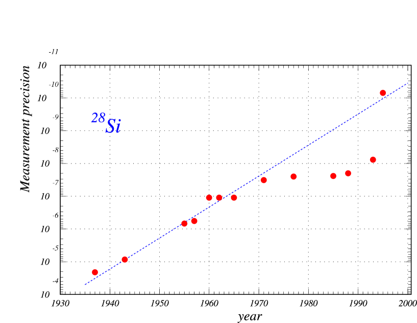
Figure 6: Our knowledge of the mass of ²⁸Si has increased by one order of magnitude per decade since 1935. Extrapolating this tendency, one could expect that we will reach a $10^{-12}$ accuracy in 2015.

3.2 Data evaluation in the Ame

The evaluation of masses share with most other evaluations many procedures. However, the very special character in the treatment of data in the mass evaluation is, as said above (header of the present Section), that all measurements are relative measurements. Each experimental datum will be thus represented by a link connecting two or three nuclei (cf. Section 3.3.1). The set of connections results in a complex canvas where data of different type and origin are entangled. Here lies the very challenge to extract values of masses from the experiments. The counterpart is that the overdetermined data system will allow cross-checks and studies of the consistencies within this system. The other help to the evaluator will be the property of regularity of the surface of masses that will be described in the last section of this lecture.

The first step in the evaluation of data is to make a compilation, i.e. a collection of all the available data. This collection must include the ‘hidden’ data: a paper does not always say clearly that some of the information it contains is of interest for mass measurement. The collection includes also even poorly documented datum, which is labelled accordingly in the Ame files.

The second step is the critical reading, which might include:

1. the evaluation or re-evaluation of the calibration procedures, the calibrators, and of the precisions of the measurements;

2. spectra examination: peaks position and relative intensities, peaks symmetry, quality of the fit;

3. search for the primary information, in the data, which do not necessarily appear always as clearly as they should. (i.e. in cases the authors combined the original result with other data, to derive a mass value, the Ame should retain only the former). It also happened that the authors gave only the derived mass value. Then the evaluator has to reconstruct the original result and ask for authors’ confirmation.

The third step in the data evaluation will be to compare the results of the examined work to earlier results if they exist (either directly, or through a combination of other data). If there are no previous results, comparison could be done with estimates from extrapolations, exploiting the above mentioned regularity of the mass surface (cf. Section  4), or to estimates from mass models or mass formulae.

Finally, the evaluator often and on has to establish a dialog with the authors of the work, asking for complementary information when necessary, or suggesting different analysis, or suggesting new measurements.

The new data can now enter the data-file as one line. For example, for the electron capture of ²⁰⁵Pb, the evaluator enters:

205 890816000c1 B  78Pe08   41.4   1.1   205Pb(e)205Tl    0.525  0.008 LM
   

where besides a 14 digits ID-number, there is a flag (as described in Ref. [3], p. 184), here ‘B’, then the Nsr reference-code [38] for the paper ‘78Pe08’ where the data appeared, the value for the $Q$ of the reaction with its error bar (41.4 $\pm$ 1.1 keV), and the reaction equation, where ‘e’ stands for electron-capture. The information in the last columns says that this datum has been derived from the intensity ratio (0.525 $\pm$ 0.008) of the L and M lines in electron capture. The evaluator can add as many comment lines as necessary, following this data line, for other information he judges useful for exchange with his fellow evaluator. Some of these comments, useful for the user of the mass tables, will appear in the Ame publication.

3.3 Data treatment

In this section, we shall first see how the network of data is built, then how the system of data can be reduced. In the third and fourth subsections, I shall describe shortly the least-squares method used in the Ame and the computer program that will decode data and calculate the adjusted masses. A fifth part will develop the very important concept of ‘Flow-of-Information’ matrix. Finally, I shall explain how checking the consistency of data (or of sub-group of data) can help the evaluator in his judgment.

3.3.1 Data entanglement - Mass Correlations

We have seen in Section 3.1 that all mass measurements are relative measurements. Each experimental piece of data can be represented by a link between two, sometimes three, and more rarely four nuclides. As mentioned earlier, assembling these links produces an extremely entangled network. A part of this network can be seen in Fig. 7.

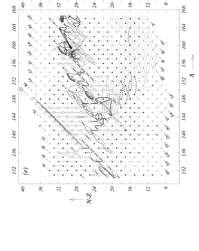
Figure 7: Diagram of connections for the experimental data. Each symbol represents one nuclide and each line represents one piece of data connecting two nuclides. When a nuclide is connected to Carbon-12 (often the case for mass spectrometry), it is represented by a square symbol.

One notices immediately that there are two types of symbols, the small and the large ones. The small ones represent the so-called secondary nuclides; while the nuclides with large symbols are called primary. Secondary nuclides are represented by full small circles if their mass is determined experimentally, and by empty ones if estimated from trends in systematics. Secondary nuclides are connected by secondary data, represented by dashed lines. A chain of dashed lines is at one end free, and at the other end connected to one unique primary nuclide (large symbol). This representation means that all secondary nuclides are determined uniquely by the chain of secondary connections going down to a primary nuclide. The latter are multiply determined and enter thus the entangled canvas. They are inter-connected by primary data, represented by full lines.

We see immediately from Fig. 7 that the mass of a primary nuclide cannot be determined straightforwardly. One may think of making an average of the values obtained from all links, but such a recipe is erroneous because the other nuclides on which these links are built are themselves inter-connected, thus not independent. In other words these primary data, connecting the primary nuclides, are correlated, and the correlation coefficients are to be taken into account.

Caveat: the word primary used for these nuclides and for the data connecting them does not mean that they are more important than the others, but only that they are subject to the special treatment below. The labels primary and secondary are not intrinsic properties of data or masses. They may change from primary to secondary or reversely when other information becomes available.

3.3.2 Compacting the set of data

We have seen that primary data are correlated. We take into account these correlations very easily with the help of the least-squares method that will be described below. The primary data will be improved in the adjustment, since each will benefit from all the available information.

Secondary data will remain unchanged; they do not contribute to $\chi^{2}$. The masses of the secondary nuclides will be derived directly by combining the relevant adjusted primary mass with the secondary datum or data. This also means that secondary data can easily be replaced by new information becoming available (but one has to watch since the replacement can change other secondary masses down the chain as seen from the diagram Fig. 7).

We define degrees for secondary masses and secondary data. They reflect their distances along the chains connecting them to the network of primaries; they range from 2 to 16. Thus, the first secondary mass connected to a primary one will be a mass of degree 2, and the connecting datum will be a datum of degree 2 too. Degree 1 is for primary masses and data.

Before treating the primary data by the least-squares method, we try as much as possible to reduce the system, but without allowing any loss of information. One way to do so is to pre-average identical data: two or more measurements of the same physical quantities can be replaced by their average value and error. Also the so-called parallel data can be pre-averaged: they are data that give essentially values for the mass difference between the same two nuclides, e.g. ⁹Be($\gamma$,n)⁸Be, ⁹Be(p,d)⁸Be, ⁹Be(d,t)⁸Be and ⁹Be(³He,$\alpha$)⁸Be. Such data are represented together, in the main least-squares calculation, by one of them carrying their average value. If the $Q$ data to be pre-averaged are strongly conflicting, i.e. if the consistency factor (or Birge ratio, or normalized $\chi$)

$$\chi_{n}=\sqrt{\frac{\chi^{2}}{Q-1}}$$ (8)

resulting in the calculation of the pre-average is greater than 2.5, the (internal) error $\sigma_{i}$ in the average is multiplied by the Birge ratio ($\sigma_{e}=\sigma_{i}\times\chi_{n}$). The quantity $\sigma_{e}$ is often called the ‘external’ error. However, this treatment is not used in the very rare cases where the errors in the values to be averaged differ too much from one another, since the assigned errors loose any significance (three cases in Ame’93). We there adopt an arithmetic average and the dispersion of values as error, which is equivalent to assigning to each of these conflicting data the same error.

In Ame’93, 28% of the 929 cases in the pre-average had values of $\chi_{n}$ beyond unity, 4.5% beyond two, 0.7% beyond 3 and only one case beyond 4, giving a very satisfactory distribution overall. With the choice above of a threshold of $\chi_{n}^{0}$=2.5 for the Birge ratio, only 1.5% of the cases are concerned by the multiplication by $\chi_{n}$. As a matter of fact, in a complex system like the one here, many values of $\chi_{n}$ beyond 1 or 2 are expected to exist, and if errors were multiplied by $\chi_{n}$ in all these cases, the $\chi^{2}$-test on the total adjustment would have been invalidated. This explains the choice made in the Ame of a rather high threshold ($\chi_{n}^{0}=2.5$), compared e.g. to $\chi_{n}^{0}$=2 recommended by Woods and Munster [39] or, even, $\chi_{n}^{0}$=1 used in a different context by the Particle Data Group [40], for departing from the rule of internal error of the weighted average (see also [41]).

Another method to increase the meaning of the final $\chi^{2}$ is to exclude data with weights at least a factor 10 less than other data, or combinations of other data giving the same result. They are still kept in the list of input data but labelled accordingly; comparison with the output values allows to check that this procedure did not have unwanted consequences.

The system of data is also greatly reduced by replacing data with isomers by an equivalent datum for the ground-state, if a $\gamma$-ray energy measurement is available from the Nndc (cf. Section 2.3). Excitation energies from such $\gamma$-ray measurements are normally far more precise than reaction energy measurements.

Typically, we start from a set of 6000 to 7000 experimental data connecting some 3000 nuclides. After pre-averaging, taking out the data with very poor accuracy and separating the secondary data, we are left with a system of 1500 primary data for 800 nuclides.

3.3.3 Least-squares method

Each piece of data has a value $q_{i}\pm dq_{i}$ with the accuracy $dq_{i}$ (one standard deviation) and makes a relation between 2, 3 or 4 masses with unknown values $m_{\mu}$. An overdetermined system of $Q$ data to $M$ masses ($Q>M$) can be represented by a system of $Q$ linear equations with $M$ parameters:

$$\sum_{\mu=1}^{M}k_{i}^{\mu}m_{\mu}=q_{i}\pm dq_{i}$$ (9)

(a generalization of Eq. 2 and Eq. 3), e.g. for a nuclear reaction $A(a,b)B$ requiring an energy $q_{i}$ to occur, the energy balance writes:

$$m_{\rm A}+m_{\rm a}-m_{\rm b}-m_{\rm B}=q_{i}\pm dq_{i}$$ (10)

thus, $k_{i}^{\rm A}=+1$,   $k_{i}^{\rm a}=+1$,   $k_{i}^{\rm B}=-1$   and   $k_{i}^{\rm b}=-1$.

In matrix notation, ${\bf K}$ being the $(Q,M)$ matrix of coefficients, Eq. 9 writes: ${\bf K}|m\rangle=|q\rangle$. Elements of matrix ${\bf K}$ are almost all null: e.g. for reaction $A(a,b)B$, Eq. 2 yields a line of ${\bf K}$ with only two non-zero elements.

We define the diagonal weight matrix ${\bf W}$ by its elements $w_{i}^{i}=1/(dq_{i}dq_{i})$. The solution of the least-squares method leads to a very simple construction:

$${\bf{}^{t}KWK}|m\rangle={\bf{}^{t}KW}|q\rangle$$ (11)

the normal matrix ${\bf A}={\bf{}^{t}KWK}$ is a square matrix of order $M$, positive-definite, symmetric and regular and hence invertible [42]. Thus the vector $|\overline{m}\rangle$ for the adjusted masses is:

$$|\overline{m}\rangle={\bf{A^{-1}}~{}^{t}KW}|q\rangle\hskip 19.91684pt{\rm or}\hskip 19.91684pt|\overline{m}\rangle={\bf R}|q\rangle$$ (12)

The rectangular $(M,Q)$ matrix ${\bf R}$ is called the response matrix.

The diagonal elements of ${\bf A^{-1}}$ are the squared errors on the adjusted masses, and the non-diagonal ones $(a^{-1})_{\mu}^{\nu}$ are the coefficients for the correlations between masses $m_{\mu}$ and $m_{\nu}$.

3.3.4 The Ame computer program

The four phases of the Ame computer program perform the following tasks:

1. decode and check the data file;

2. build up a representation of the connections between masses, allowing thus to separate primary masses and data from secondary ones and then to reduce drastically the size of the system of equations to be solved, without any loss of information;

3. perform the least-squares matrix calculations (see above); and

4. deduce the atomic masses, the nuclear reaction and separation energies, the adjusted values for the input data, the influences of data on the primary masses described in next section, and display information on the inversion errors, the correlations coefficients, the values of the $\chi^{2}$ (cf. Section 3.3.6), and the distribution of the normalized deviations $v_{i}$.

3.3.5 Flow-of-Information

One of the most powerful tools in the least-squares calculation described above is the flow-of-information matrix. This matrix allows to trace back, in the least-squares method, the contribution of each individual piece of data to each of the parameters (here the atomic masses). The Ame uses this method since 1993.

The flow-of-information matrix ${\bf F}$ is defined as follows: ${\bf K}$, the matrix of coefficients, is a rectangular $(Q,M)$ matrix, the transpose of the response matrix ${\bf{}^{t}R}$ is also a $(Q,M)$ rectangular one. The $(i,\mu)$ element of ${\bf F}$ is defined as the product of the corresponding elements of ${\bf{}^{t}R}$ and of ${\bf K}$. In reference [43] it is demonstrated that such an element represents the “influence” of datum $i$ on parameter (mass) $m_{\mu}$. A column of ${\bf F}$ thus represents all the contributions brought by all data to a given mass $m_{\mu}$, and a line of ${\bf F}$ represents all the influences given by a single piece of data. The sum of influences along a line is the “significance” of that datum. It has also been proven [43] that the influences and significances have all the expected properties, namely that the sum of all the influences on a given mass (along a column) is unity, that the significance of a datum is always less than unity and that it always decreases when new data are added. The significance defined in this way is exactly the quantity obtained by squaring the ratio of the uncertainty on the adjusted value over that on the input one, which is the recipe that was used before the discovery of the ${\bf F}$ matrix to calculate the relative importance of data.

A simple interpretation of influences and significances can be obtained in calculating, from the adjusted masses and Eq. 9, the adjusted data:

$$|\overline{q}\rangle={\bf KR}|q\rangle.$$ (13)

The $i^{th}$ diagonal element of ${\bf KR}$ represents then the contribution of datum $i$ to the determination of $\overline{q_{i}}$ (same datum): this quantity is exactly what is called above the significance of datum $i$. This $i^{th}$ diagonal element of ${\bf KR}$ is the sum of the products of line $i$ of ${\bf K}$ and column $i$ of ${\bf R}$. The individual terms in this sum are precisely the influences defined above.

The flow-of-information matrix ${\bf F}$, provides thus insight on how the information from datum $i$ flows into each of the masses $m_{\mu}$.

3.3.6 Consistency of data

The system of equations being largely over-determined ($Q>>M$) offers the evaluator several interesting possibilities to examine and judge the data. One might for example examine all data for which the adjusted values deviate importantly from the input ones. This helps to locate erroneous pieces of information. One could also examine a group of data in one experiment and check if the errors assigned to them in the experimental paper were not underestimated.

If the precisions $dq_{i}$ assigned to the data $q_{i}$ were indeed all accurate, the normalized deviations $v_{i}$ between adjusted $\overline{q}_{i}$ and input $q_{i}$ data (cf. Eq. 13), $v_{i}=(\overline{q}_{i}-q_{i})/dq_{i}$, would be distributed as a gaussian function of standard deviation $\sigma=1$, and would make $\chi^{2}$:

$$\chi^{2}=\sum_{i=1}^{Q}\left(\frac{\overline{q}_{i}-q_{i}}{dq_{i}}\right)^{2}\hskip 19.91684pt{\rm or}\hskip 19.91684pt\chi^{2}=\sum_{i=1}^{Q}v_{i}^{2}$$ (14)

equal to $Q-M$, the number of degrees of freedom, with a precision of $\sqrt{2(Q-M)}$.

One can define as above the normalized chi, $\chi_{n}$ (or ‘consistency factor’ or ‘Birge ratio’): $\chi_{n}=\sqrt{\chi^{2}/(Q-M)}$ for which the expected value is $1\pm 1/\sqrt{2(Q-M)}$.

For our current Ame2003 example of 1381 equations with 847 parameters, i.e. 534 degrees of freedom, the theoretical expectation value for $\chi^{2}$ should be 534$\pm$33 (and the theoretical $\chi_{n}=1\pm 0.031$). The total $\chi^{2}$ of the adjustment is actually 814; this means that, in the average, the errors in the input values have been underestimated by 23%, a still acceptable result. In other words, the experimentalists measuring masses were, on average, too optimistic by 23%. The distribution of the $v_{i}$’s (the individual contributions to $\chi^{2}$, as defined in Eq. 14 is also acceptable, with, in Ame2003, 15% of the cases beyond unity, 3.2% beyond two, and 8 items (0.007%) beyond 3.

The $\chi_{n}$ value was 1.062 in Ame’83 for $Q-M$=760 degrees of freedom, 1.176 in Ame’93 for $Q-M=635$, and 1.169 in the Ame’95 update for $Q-M$=622.

Another quantity of interest for the evaluator is the partial consistency factor, $\chi_{n}^{p}$, defined for a (homogeneous) group of $p$ data as:

$$\chi_{n}^{p}=\sqrt{\frac{Q}{Q-M}\phantom{0}\frac{1}{p}\phantom{0}\sum_{i=1}^{p}v_{i}^{2}}.$$ (15)

Of course the definition is such that $\chi_{n}^{p}$ reduces to $\chi_{n}$ if the sum is taken over all the input data.

One can consider for example the two main classes of data: the reaction and decay energy measurements and the mass spectrometric data (see Section 3.1). The partial consistency factors $\chi_{n}^{p}$ are respectively 1.269 and 1.160 for energy measurements and for mass spectrometry data, showing that both types of input data are responsible for the underestimated error of 23% mentioned above, with a better result for mass spectrometry data.

One can also try to estimate the average accuracy for 181 groups of data related to a given laboratory and with a given method of measurement, by calculating their partial consistency factors $\chi_{n}^{p}$. A high value of $\chi_{n}^{p}$ might be a warning on the validity of the considered group of data within the reported errors. In general, in the Ame such a situation is extremely rare, because deviating data are cured before entering the ‘machinery’ of the adjustment, at the stage of the evaluation itself (see Section 3.2). On the average the experimental errors appear to be slightly underestimated, with as much as 57% (instead of expected 33%) of the groups of data having $\chi_{n}^{p}$ larger than unity. Agreeing better with statistics, 5.5% of these groups are beyond $\chi_{n}^{p}=2$.

3.4 Data requiring special treatment

It often happens that data require some special treatment before entering the data-file (cf. Section 3.2). Such is the case of data given with asymmetric uncertainties, or when information is obtained only as one lower and one upper limit, defining thus a range of values. We shall examine these two cases.

All errors entering the data-file must be one standard deviation (1 $\sigma$) errors. When it is not the case, they must be converted to 1 $\sigma$ errors to allow combination with other data.

3.4.1 Asymmetric errors

Sometimes the precision on a measurement is not given as a single number, like $\sigma$ (or $dq$ in Section 3.3.3 above), but asymmetrically $X^{+a}_{-b}$, as shown in Fig. 8.

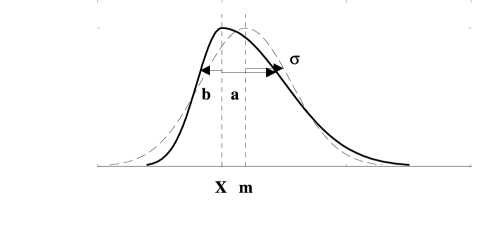
Figure 8: An experimental result is represented by an asymmetric probability density function (heavy solid line) with central value $X$ and errors $+a$ and $-b$. This function is symmetrized as shown by the dashed line with its center $m$ displaced by $0.64\cdot(a-b)$

Such errors are symmetrized, before entering the treatment procedure. A rough estimate can be used: take the central value to be the mid-value between the upper and lower 1$\sigma$-equivalent limits $X+(a-b)/2$, and define the uncertainty to be the average of the two uncertainties $(a+b)/2$. A better approximation is obtained with the recipe described in Ref. [5]. The central value $X$ is shifted to:

$$X+0.64\cdot(a-b)$$ (16)

and the precision $\sigma$ is:

$$\sigma^{2}=(1-\frac{2}{\pi})\,(a-b)^{2}+ab.$$ (17)

In the appendix of Ref. [5] one can find the demonstration and discussion of Eq. 16 and Eq. 17.

3.4.2 Range of values

Some measurements are reported as a range of values with most probable lower and upper limits (Fig. 9). They are treated as a uniform distribution of probabilities [44]. The moments of this distribution yield a central value at the middle of the range and a 1$\sigma$ uncertainty of 29% of that range.

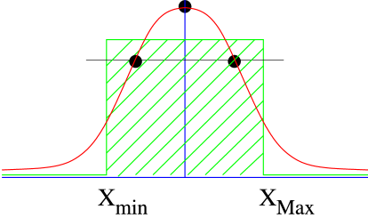
Figure 9: Experimental datum given as a range of values is represented by a rectangular distribution of probabilities.

3.4.3 Mixture of spectral lines

**** to be completed ****

4 Regularity of the mass-surface

When nuclear masses are displayed as a function of $N$ and $Z$, one obtains a surface in a 3-dimensional space. However, due to the pairing energy, this surface splits into four sheets. The even-even sheet lies lowest, the odd-odd highest, the other two nearly halfway between as represented in Fig. 10.

Figure 10: The surface of masses is split into four sheets. This scheme represents the pairing energies responsible for this splitting. The zero energy surface is a purely hypothetical one for no pairing at all among the last nucleons.

The vertical distances from the even-even sheet to the odd-even and even-odd ones are the proton and neutron pairing energies $\Delta_{pp}$ and $\Delta_{nn}$. They are nearly equal. The distances of the last two sheets to the odd-odd sheet are equal to $\Delta_{nn}-\Delta_{np}$ and $\Delta_{pp}-\Delta_{np}$, where $\Delta_{np}$ is the proton-neutron pairing energy due to the interaction between the two odd nucleons, which are generally not in the same shell. These energies are represented in Fig. 10, where a hypothetical energy zero represents a nuclide with no pairing among the last nucleons.

Experimentally, it has been observed that:

• the four sheets run nearly parallel in all directions, which means that the quantities $\Delta_{nn}$, $\Delta_{pp}$ and $\Delta_{np}$ vary smoothly and slowly with $N$ and $Z$; and

• each of the mass sheets varies very smoothly also, but very rapidly. with $N$ and $Z$. The smoothness is also observed for first order derivatives (slopes, cf. Section 4.2.1) and all second order derivatives (curvatures of the mass surface). They are only interrupted in places by sharp cusps or large depressions associated with important changes in nuclear structure: shell or sub-shell closures (sharp cusps), shape transitions (spherical-deformed, prolate-oblate: depressions on the mass surface), and the so-called ‘Wigner’ cusp along the $N=Z$ line.

This observed regularity of the mass sheets in all places where no change in the physics of the nucleus are known to exist, can be considered as one of the basic properties of the mass surface. Thus, dependable estimates of unknown, poorly known or questionable masses can be obtained by extrapolation from well-known mass values on the same sheet. Examination of previous such estimates, where the masses are now known, shows that the method used, though basically simple, has a good predictive power [36].

In the evaluation of masses the property of regularity and the possibility to make estimates are used for several purposes:

1. New Physics - Any coherent deviation from regularity, in a region $(N,Z)$ of some extent, could be considered as an indication that some new physical property is being discovered.

2. Outliers - However, if one single mass violates the systematic trends, then one may seriously question the correctness of the related datum. There might be, for example, some undetected systematic [45] contribution to the reported result of the experiment measuring this mass. We then reread the experimental paper with extra care for possible uncertainties, and often ask the authors for further information. This often leads to corrections.
   In the case where a mass determined from only one experiment (or from same experiments) deviate severely from the smooth surface, replacement by an estimated value would give a more usefull information to the user of the tables and would prevent obscuring the plots for the observation of the mass surface. Fig. 11 for one of the derivatives of the mass surface (cf. Section 4.2.1) is taken from Ame’93 and shows how replacements of a few such data by estimated values, can repair the surface of masses in a region, not so well known, characterized by important irregularities. Presently, only the most striking cases, not all irregularities, have been replaced by estimates: typically those that obscure plots like in Fig. 11.

   

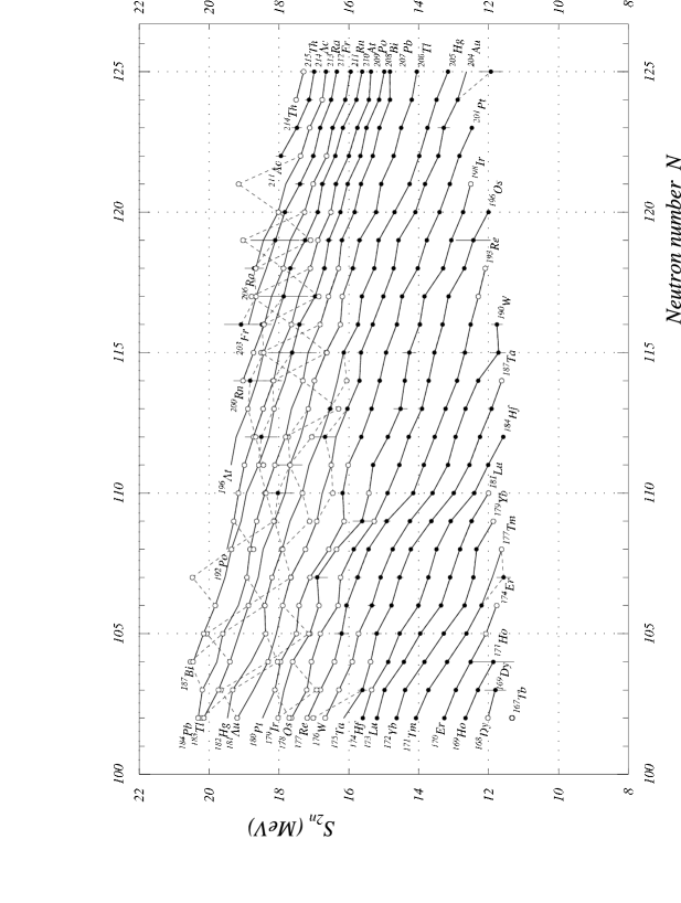
   Figure 11: Two-neutron separation energies as a function of $N$ (from Ame’93, p. 166). Solid points and error bars represent experimental values, open circles represent masses estimated from “trends in systematics”. Replacing some of the experimental data by values estimated from these trends, changes the mass surface from the dotted to the full lines. The use of a ‘derivative’ function adds to the confusion of the dotted lines, since two points are changed if one mass is displaced. Moreover, in this region there are many $\alpha$ links resulting in large propagation of errors.

3. Conflicts among data - There are cases where some experimental data on the mass of a particular nuclide disagree among each other and no particular reason for rejecting one or some of them could be found from studying the involved papers. In such cases, the measure of agreement with the just mentioned regularity can be used by the evaluators for selecting which of the conflicting data will be accepted and used in the evaluation.

4. Estimates - Finally, drawing the mass surface allows to derive estimates for the still unknown masses, either from interpolations or from short extrapolations, as can be seen in Fig. 12.

   

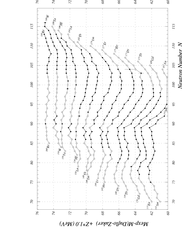
   Figure 12: Differences, in the rare-earth region, between the masses and the values predicted by the model of Duflo and Zuker [46]. Open circles represent values estimated from systematic trends; points are for experimental values.

4.1 Extrapolations

In the case of extrapolation however, the error in the estimated mass will increase with the distance of extrapolation. These errors are obtained by considering several graphs of systematics with a guess on how much the estimated mass may change without the extrapolated surface looking too much distorted. This recipe is unavoidably subjective, but has proven to be efficient through the agreement of these estimates with newly measured masses in the great majority of cases.

It would be desirable to give estimates for all unknown nuclides that are within reach of the present accelerator and mass separator technologies. But, in fact, the Ame only estimates values for all nuclides for which at least one piece of experimental information is available (e.g. identification or half-life measurement or proof of instability towards proton or neutron emission). In addition, the evaluators want to achieve continuity in $N$, in $Z$, in $A$ and in $N-Z$ of the set of nuclides for which mass values are estimated. This set is therefore the same as the one defined for Nubase [5].

To be complete, it should be said that regularity is not the only property used to make estimates: all available experimental information is taken into account. The limits for the methods based on regularity appear rapidly when going down to low mass numbers where nuclear structures appear and disappear on very short ranges, not to mention vanishing magic numbers.

Neutron-rich masses could be constrained by our knowledge of nuclides being stable or unstable relative to neutron emission: e.g. stability against neutron emission implies a positive neutron separation energie. This property, however, is usefull only for light species, where the neutron drip-line can be reached. Similarly for proton-rich nuclides, but here one has to be carefull and take into account the Coulomb barrier which may hinder proton emission of a slightly p-unbound nucleus. Light proton-rich masses could be derived from the masses of their mirror companions, or from the Imme (Isobaric Multiplet Mass Equation) which showed, up to now, to be fairly well verified. New developments in these directions are in progress.

4.2 Scrutinizing the surface of masses

Direct representation of the mass surface is not convenient since the binding energy varies very rapidly with $N$ and $Z$. Splitting in four sheets, as mentioned above, complicates even more such a representation. There are two ways to still be able to observe with some precision the surface of masses: one of them uses the derivatives of this surface, the other is obtained by subtracting a simple function of $N$ and $Z$ from the masses.

They are both described below and I will end this section with a description of the interactive computer program that visualizes all these functions to allow easier derivation of the estimated values.

4.2.1 The derivatives of the mass surface

By derivative of the mass surface we mean a specified difference between the masses of two nearby nuclei. These functions are also smooth and have the advantage of displaying much smaller variations. For a derivative specified in such a way that differences are between nuclides in the same mass sheet, the near parallelism of these leads to an (almost) unique surface for the derivative, allowing thus a single display. Therefore, in order to illustrate the systematic trends of the masses, four derivatives of this last type were traditionally chosen:

1. the two-neutron separation energies versus $N$, with lines connecting the isotopes of a given element, as in Fig. 11;

2. the two-proton separation energies versus $Z$, with lines connecting the isotones (the same number of neutrons);

3. the $\alpha$-decay energies versus $N$, with lines connecting the isotopes of a given element; and

4. the double $\beta$-decay energies versus $A$, with lines connecting the isotopes and the isotones.

These four derivatives are given in the printed version of the Ame2003, Part II, Figs. 1–36 [4].

However, from the way these four derivatives are built, they give only information within one of the four sheets of the mass surface (e-e, e-o, o-e or e-e; e-o standing for even $N$ and odd $Z$). When observing the mass surface, an increased or decreased spacing of the sheets cannot be observed. Also, when estimating unknown masses, divergences of the four sheets could be unduly created, which is unacceptable.

Fortunately, other various representations are possible (e.g. separately for odd and even nuclei: one-neutron separation energies versus $N$, one-proton separation energy versus $Z$, $\beta$-decay energy versus $A$, …). Such graphs have been prepared and can be obtained from the Amdc web distribution [47].

The method of ‘derivatives’ suffers from involving two masses for each point to be drawn, which means that if one mass is moved then two points are changed in opposite direction, causing confusion in our drawings Fig. 11.

4.2.2 Subtracting a simple function

Since the mass surface is smooth, one can try to define a function of $N$ and $Z$ as simple as possible and not too far from the real surface of masses. The difference between the mass surface and this function, while displaying reliably the structure of the former, will vary much less rapidly, improving thus its observation.

Subtracting results from a model

Practically, we use the results of the calculation of one of the modern models. However, we can use here only those models that provide masses specifically for the spherical part, forcing the nucleus to be un-deformed. The reason is that the models generally describe quite well the shell and sub-shell closures, and to some extent the pairing energies, but not the locations of deformation. If the theoretical deformations were included and not located at exactly the same position as given by the experimental masses, the mass difference surface would show two dislocations for each shape transition. Interpretation of the resulting surface would then be very difficult.

My two choices are the “New Semi-Empirical Shell Correction to the Droplet Model (Gross Theory of Nuclear Magics)” by Groote, Hilf and Takahashi [48]; and the “Microscopic Mass Formulas” of Duflo and Zuker [46], which has been illustrated above (Fig. 12). In Ame2003, we made extensive use of such differences with models. The plots we have prepared were not published, they can be retrieved from the Amdc [47].

The difference of mass surfaces shown in Fig. 12 is instructive:

1. the lines for the isotopic series cross the $N$=82 shell closure with almost no disruption, showing thus how well shell closures are described by the model;

2. the well-known onset of deformation in the rare-earth at $N$=90 appears very clearly here as a deep large bowl, since deformation is not used in this calculation. The contour of this deformation region is neat. The depth, i.e. the amount of energy gained due to deformation, compared to ideal spherical nuclides, can be estimated; and

3. Fig. 12 shows also how the amplitude of deformation decreases with increasing $Z$ and seems to vanish when approaching Rhenium ($Z$=75).

Subtracting a Bethe and Weizsäcker formula

Since 1975 [49], and now with more and more evidence, it appears that the ‘magic’ numbers that were though to occur at fixed numbers of protons or neutrons, are not really so. They might disappear when going away from the valley of stability, or appear at new locations. Where such migrations occur, most models are much in trouble, and the reasoning we made above for not including deformation in the models, now applies also to ‘magic’ numbers. Excluding shell and sub-shell closures, we are then driven directly back to the pioneering work of Weizsäcker [50]. Recent works [51, 52] on the modern fits of the original Bethe and Weizsäcker’s formula seems promising in this respect.

The concept of the liquid drop mass formula was defined by Weizsäcker in 1935 [50] and fine-tuned by Bethe and Bacher [53] in 1936. The binding energy of the nucleus comprises only a volume energy term, a surface one, an asymmetry term, and the Coulomb energy contribution for the repulsion amongst protons. The total mass is thus:

$${\cal M}(N,Z)=N{\cal M}_{\rm n}+Z{\cal M}_{\rm H}-\alpha A+\beta\frac{(N-Z)^{2}}{A}+\gamma A^{2\over 3}+\frac{3}{5}\frac{e^{2}Z^{2}}{r_{0}A^{1\over 3}}$$ (18)

where $A=N+Z$, is the atomic weight, $r_{0}A^{1/3}$ the nuclear radius, ${\cal M}_{\rm n}$ and ${\cal M}_{\rm H}$ the masses of the neutron and of the hydrogen atom. The constants $\alpha$, $\beta$, $\gamma$ and $r_{0}$ were determined empirically by Bethe and Bacher: $\alpha=13.86$ MeV, $\beta=19.5$ MeV, $\gamma=13.2$ MeV and $r_{0}=1.48\cdot 10^{-15}$ m (then $\frac{3}{5}e^{2}/r_{0}=0.58$ MeV). The formula of Eq. (18) is unchanged if ${\cal M}(N,Z)$, ${\cal M}_{\rm n}$ and ${\cal M}_{\rm H}$ are replaced by their respective mass excesses (at that time they were called mass defects). When using the constants given above one should be aware that when Bethe fixed them, he used for the mass excesses of the neutron and hydrogen atom respectively 7.8 MeV and 7.44 MeV in the ¹⁶O standard, with a value of 930 MeV for the atomic mass unit.

If we subtract Eq. (18) from all masses we are left with values that vary much less rapidly than the masses themselves, while still showing all the structures. However, the splitting in four sheets will still make the image fuzzy. One can then add to the right hand side of the formula of Bethe (18) a commonly used pairing term $\Delta_{pp}=\Delta_{nn}=-12/\sqrt{A}$ MeV and no $\Delta_{np}$ (Fig. 10), which is sufficient for our purpose. (For those interested, there is a more refined study of the variations of the pairing energies that has been made by Jensen, Hansen and Jonson [54]).

4.3 Far extrapolations

When exploiting these observations one can make extrapolations for masses very far from stability. This has been done already [55], but with a further refinement of this method obtained by constructing an idealized surface of masses (or mass-geoid) [56], which is the best possible function to be subtracted from the mass surface. In Ref. [55], a local mass-geoid was built as a cubic function of $N$ and $Z$ in a region limited by magic numbers for both $N$ and $Z$, fitted to only the purely spherical nuclides and keeping only the very reliable experimental masses. Then the shape of the bowl (for deformation) was reconstructed ‘by hand’, starting from the known non-spherical experimental masses. It was found that the maximum amplitude of deformation amounts to 5 MeV, is located at ¹⁶⁸Dy, and that the region of deformation extends from $N$=90 to $N$=114 and from $Z$=55 to $Z$=77, which is roughly in agreement with what is indicated by Fig. 12.

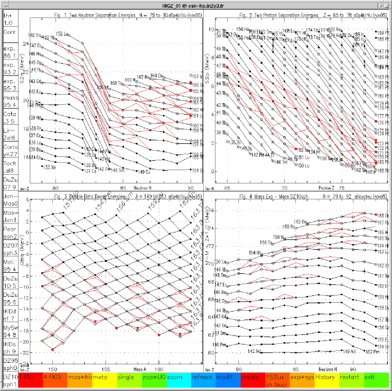
Figure 13: A screen image of Desint, the interactive graphical display of four cuts in the surface of masses around ¹⁴⁶Gd. The four quadrants display respectively $S_{2n}(N)$, $S_{2p}(Z)$, $Q_{2\beta}(A)$ and $(M_{\rm exp}-M_{\rm Duflo-Zuker})(N)$ [46]. The lines in black connect nuclides with same $Z$, $N$, ($Z$ and $N$) and $Z$ respectively. The boxes at left and bottom serve for various interactive commands. The $N$=82 shell closure is clearly seen in quadrant 1 and in the lower left corner of quadrant 3. The lines in red illustrate the many consequences of an increase of the mass of ¹⁴⁶Gd by 500 keV.

4.4 Manipulating the mass surface

In order to make estimates of unknown masses or to test changes on measured ones, one needs to visualize different graphs, either from the ‘derivatives’ type or from the ‘difference’ type. On these graphs, one needs to add (or move) the relevant mass and determine how much freedom is left in setting a value for this mass.

Things are still more complicated, particularly for changes on measured masses, since other masses could depend on the modified one, usually through secondary data. Then one mass change may give on one graph several connected changes.

Another difficulty is that a mass modification (or a mass creation) may look acceptable on one graph, but may appear unacceptable on another graph. One should therefore be able to watch several graphs at the same time.

A supplementary difficulty may appear in some types of graphs where two tendencies may alternate, following the parity of the proton or of the neutron numbers. One may then wish, at least for better comfort, to visualize only one of these two parities.

All this has become possible with the ‘interactive graphical tool’, called Desint (from the French: ‘dessin interactif’) written by C. Borcea [57] and illustrated in Fig. 13. Any of the ‘derivatives’ or of the ‘differences’ can be displayed in any of the four quadrants of Fig. 13, or alone and enlarged. Any of these functions can be plotted against any of the parameters $N$, $Z$, $A$, $N-Z$, and $2Z-N$; and connect iso-lines in any single or double parameters of the same list (e.g., in the third view of Fig. 13, iso-lines are drawn for $Z$ and for $N$). Zooming in and out to any level and moving along the two coordinates are possible independently for each quadrant. Finally, and more importantly, any change appears, in a different color, with all its consequences and in all four graphs at the same time. As an example and only for the purpose of illustration, a change of +500 keV has been applied, in Fig. 13, to ¹⁴⁶Gd in quadrant number four; all modifications in all graphs appear in red.

5 The Tables

In December 2003, we succeeded in having published together the “Atomic Mass Evaluation” Ame [3, 4] and the Nubase evaluation [5], which have the same “horizontal” structure and basic interconnections at the level of isomers.

After the 1993 tables (Ame’93) it was projected to have updated evaluations performed regularly (every two years) and published in paper only partly, while all files should still be distributed on the Web. Effectively, an update Ame’95 [2] appeared two years later. Lack of time to evaluate the stream of new quite important data, and also the necessity to create the Nubase evaluation (see below), prevented the intended further updates of the Ame. The Nubase evaluation was thus published for the first time in September 1997 [6], but in order to have consistency between the two tables, it was decided then that the masses in Nubase’97 should be exactly those from Ame’95. A certain stabilization, that seems to be reached now, encouraged us to publish in 2003 a new full evaluation of masses, together with the new version of Nubase. This time, the Ame2003 and Nubase2003 are completely ‘synchronized’.

Full content of the two evaluations is accessible on-line at the web site of the Atomic Mass Data Center (Amdc) [58] through the World Wide Web. One will find at the Amdc, not only the published material, but also extra figures, tables, documentation, and more specially the Ascii files for the Ame2003 and the Nubase2003 tables, for use with computer programs.

The contents of Nubase can be displayed with a PC-program called “Nucleus” [59], and also by a Java program jvNubase [60] through the World Wide Web, both distributed by the Amdc.

6 Conclusion

Deriving a mass value for a nuclide from one or several experiments is in most cases not easy. Some mathematical tools (the least-squares method) and computer tools (interactive graphical display), and especially the evaluator’s judgment are essential ingredients to reach the best possible recommended values for the masses.

Unknown masses close to the last known ones can be predicted from the extension of the mass surface. However, for the ones further out, more particularly those which are essential in many astrophysical problems, like the nucleosynthesis r-process, values for the masses can only be derived from some of the available models. Unfortunately, the latter exhibit very large divergences among them when departing from the narrow region of known masses, reaching up to tens of MeV’s in the regions of the r-process paths. Therefore, one of the many motivations for the best possible evaluation of masses is to get the best set of mass values on which models may adjust their parameters and better predict masses further away.

References

-
[1]
T.W. Burrows,
Nucl. Instrum. Meth. A 286 (1990) 595;
http://www.nndc.bnl.gov/nndc/ensdf/. - [2] G. Audi and A.H. Wapstra, Nucl. Phys. A 595 (1995) 409.
- [3] A.H. Wapstra, G. Audi and C. Thibault, Nucl. Phys. A 729 (2003) 129.
- [4] G. Audi, A.H. Wapstra and C. Thibault, Nucl. Phys. A 729 (2003) 337.
- [5] G. Audi, O. Bersillon, J. Blachot and A.H. Wapstra, Nucl. Phys. A 729 (2003) 3.
- [6] G. Audi, O. Bersillon, J. Blachot and A.H. Wapstra, Nucl. Phys. A 624 (1997) 1.
- [7] R.J. Irvine, C.N. Davids, P.J. Woods, D.J. Blumenthal, L.T. Brown, L.F. Conticchio, T. Davinson, D.J. Henderson, J.A. Mackenzie, H.T. Penttilä, D. Seweryniak and W.B. Walters, Phys. Rev. C 55 (1997) 1621.
- [8] T. Morek, K. Starosta, Ch. Droste, D. Fossan, G. Lane, J. Sears, J. Smith and P. Vaska, Eur. Phys. Journal A 3 (1998) 99.
- [9] C.J. Gallagher, Jr. and S.A. Moszkowski, Phys. Rev.111 (1958) 1282.
- [10] E.W. Otten, Treatise on Heavy-Ion Science, ed. D.A. Bromley 8, 517 (1989).
- [11] P. Aufmuth, K. Heilig and A. Steudel, At. Nucl. Data Tables 37 (1987) 455.
- [12] P. Raghavan, At. Nucl. Data Tables 42 (1989) 189.
- [13] N. Stone, At. Nucl. Data Tables to be published (1999).
- [14] I. Angeli, Acta Phys. Hungarica 69 (1991) 233.
- [15] E.G. Nadjakov, K.P. Marinova and Yu.P. Gangrsky, At. Nucl. Data Tables 56 (1994) 133.
- [16] N.E. Holden, Report BNL-61460 (1995).
- [17] S. Raman, C.W. Nestor, Jr., S. Kahane and K.H. Bhatt, At. Nucl. Data Tables 42 (1989) 1.
-
[18]
A. Lépine-Szily,
Experimental Overview of Mass Measurements, tutorial lecture at the
Second Euroconference on Atomic Physics at Accelerators - Mass Spectrometry (Apac-2000), Cargèse (France), 18-23 Septembre 2000, Hyperfine Interactions 132 (2001) 35-57. - [19] T.P. Kohman, J.H.E. Mattauch and A.H. Wapstra, J. de Chimie Physique 55 (1958) 393.
- [20] John Dalton, 1766-1844, who first speculated that elements combine in proportions following simple laws, and was the first to create a table of (very approximate) atomic weights.
- [21] P.J. Mohr and B.N. Taylor, J. Phys. Chem. Ref. Data 28 (1999) 1713.
- [22] E.R. Cohen and A.H. Wapstra, Nucl. Instrum. Meth. 211 (1983) 153.
- [23] A.H. Wapstra and K. Bos, At. Nucl. Data Tables 20 (1977) 1.
- [24] V.T. Koslowsky, J.C. Hardy, E. Hagberg, R.E. Azuma, G.C. Ball, E.T.H. Clifford, W.G. Davies, H. Schmeing, U.J. Schrewe and K.S. Sharma, Nucl. Phys. A 472 (1987) 419.
- [25] E.G. Kessler, Jr., M.S. Dewey, R.D. Deslattes, A. Henins, H.G. Börner, M. Jentschel, C. Doll and H. Lehmann, Phys. Lett. A 255 (1999) 221.
- [26] C.N. Davids, P.J. Woods, H.T. Penttilä, J.C. Batchelder, C.R. Bingham, D.J. Blumenthal, L.T. Brown, B.C. Busse, L.F. Conticchio, T. Davinson, D.J. Henderson, R.J. Irvine, D. Seweryniak, K.S. Toth, W.B. Walters and B.E. Zimmerman, Phys. Rev. Lett. 76 (1996) 592.
- [27] R.R. Ries, R.A. Damerow, W.H. Johnson, Proc. 2nd Int. Conf. Atomic Masses and Fund. Constants (Amco-2), Vienna, July 1963, p. 357.
- [28] R.C. Barber, R.L. Bishop, L.A. Cambey, H.E. Duckworth, J.D. Macdougall, W. McLatchie, J.H. Ormrod and P. Van Rookhuyzen, Proc. 2nd Int. Conf. Atomic Masses and Fund. Constants (Amco-2), Vienna, July 1963, p. 393.
-
[29]
A. Gillibert, W. Mittig, L. Bianchi, A. Cunsolo, B. Fernandez, A. Foti, J. Gastebois, C. Grégoire, Y. Schutz and C. Stephan,
Phys. Lett. B 192 (1987) 39;
D.J. Vieira, J.M. Wouters, K. Vaziri, R.H. Krauss, Jr., H. Wollnik, G.W. Butler, F.K. Wohn and A.H. Wapstra, Phys. Rev. Lett. 57 (1986) 3253. - [30] M. Chartier, G. Auger, W. Mittig, A. Lépine-Szilly, L.K. Fifield, J.M. Casandjian, M. Chabert, J. Ferme, A. Gillibert, M. Lewitowicz, M. Mac Cormick, M.H. Moscatello, O.H. Odland, N.A. Orr, G. Politi, C. Spitaels and A.C.C. Villari, Phys. Rev. Lett. 77 (1996) 2400.
- [31] J. Trötscher, K. Balog, H. Eickhoff, B. Franczak, B. Franzke, Y. Fujita, H. Geissel, Ch. Klein, J. Knollmann, A. Kraft, K.E.G. Löbner, A. Magel, G. Münzenberg, A. Przewloka, D. Rosenauer, H. Schäfer, M. Sendor, D.J. Vieira, B. Vogel, Th. Winkelmann and H. Wollnik, Nucl. Instrum. Meth. B 70 (1992) 455.
-
[32]
L.G. Smith and C.C. Damm,
Rev. Sci. Instr. 27 (1956) 638;
L.G. Smith, Phys. Rev.111 (1958) 1606. -
[33]
P.B. Schwinberg, R.S. Van Dyck, Jr. and R.S. Dehmelt,
Phys. Lett. A 81 (1981) 119;
for a recent review: D. Lunney, Mesures des propriétés statiques des noyaux : utilisation des pièges ioniques, notes de l’École Joliot-Curie de Physique Nucléaire (1999) 85. - [34] B. Franzke, K. Beckert, H. Eickhoff, F. Nolden, H. Reich, U. Schaaf, B. Schlitt, A. Schwinn, M. Steck and Th. Winkler, Phys. Scr. T59 (1994) 176.
- [35] K.-N. Huang, M. Aoyagi, M.H. Chen, B. Crasemann and H. Mark, At. Nucl. Data Tables 18 (1976) 243.
- [36] D. Lunney, J.M. Pearson and C. Thibault, Rev. Mod. Phys. 75 (2003) 1021.
- [37] F. DiFilippo, V. Natarajan, M. Bradley, F. Palmer and D.E. Pritchard, Phys. Scr. T59 (1995) 144.
- [38] Nuclear Structure Reference (Nsr): a computer file of indexed references maintained by NNDC, Brookhaven National Laboratory; http://ndcnt1.dne.bnl.gov/nsrq/ or http://www.nndc.bnl.gov/.
- [39] M.J. Woods and A.S. Munster, NPL Report RS(EXT) 95 (1988).
- [40] Particle Data Group, ‘Review of Particle Properties’, Eur. Phys. Journal C 3 (1998), 1.
- [41] A.H. Wapstra, Inst. Phys. Conf. Series 132 (1993) 129.
- [42] Y.V. Linnik, Method of Least Squares (Pergamon, New York, 1961); Méthode des Moindres Carrés (Dunod, Paris, 1963)
- [43] G. Audi, W.G. Davies and G.E. Lee-Whiting, Nucl. Instrum. Meth. A 249 (1986) 443.
- [44] G. Audi, M. Epherre, C. Thibault, A.H. Wapstra and K. Bos, Nucl. Phys. A 378 (1982) 443.
- [45] Systematic errors are those due to instrumental drifts or instrumental fluctuations, that are beyond control and are not accounted for in the error budget. They might show up in the calibration process, or when the measurement is repeated under different experimental conditions. The experimentalist adds then quadratically a systematic error to the statistical and the calibration ones, in such a way as to have consistency of his data. If not completely accounted for or not seen in that experiment, they can still be observed by the mass evaluators when considering the mass adjustment as a whole.
- [46] J. Duflo and A.P. Zuker, Phys. Rev. C 52 (1995) 23; and private communication February 1996 to the Amdc, http://www.nndc.bnl.gov/amdc/theory/du_zu_10.feb96.
- [47] http://www.nndc.bnl.gov/amdc/masstables/Ame2003/graphs2003/
- [48] H.v. Groote, E.R. Hilf and K. Takahashi, At. Nucl. Data Tables 17 (1976) 418.
- [49] C. Thibault, R. Klapisch, C. Rigaud, A.M. Poskanzer, R. Prieels, L. Lessard and W. Reisdorf, Phys. Rev. C 12 (1975) 644.
- [50] C.F. von Weizsäcker, Z. Phys. 96 (1935) 431.
- [51] Julian Michael Fletcher, M.Sc. dissertation, University of Surrey, September 2003.
- [52] Piet J. van Isacker, private communication, June 2004.
- [53] H.A. Bethe and R.F. Bacher, Rev. Mod. Phys. 8 (1936) 82.
- [54] A.S. Jensen, P.G. Hansen and B. Jonson, Nucl. Phys. A 431 (1984) 393.
- [55] C. Borcea and G. Audi, AIP Conf. Proc. 455 (1998) 98.
- [56] C. Borcea and G. Audi, Proc. Int. Conf. on Exotic Nuclei and Atomic Masses (Enam’95), Arles, June 1995, p. 127.
- [57] C. Borcea and G. Audi, Rev. Roum. Phys. 38 (1993) 455; Report CSNSM 92-38, October 1992, http://www.nndc.bnl.gov/amdc/extrapolations/bernex.pdf.
- [58] The Nubase and the Ame files in the electronic distribution can be retrieved from the Atomic Mass Data Center through the Web at http://www.nndc.bnl.gov/amdc/.
- [59] B. Potet, J. Duflo and G. Audi, Proc. Int. Conf. on Exotic Nuclei and Atomic Masses (Enam’95), Arles, June 1995, p. 151; http://www.nndc.bnl.gov/amdc/nucleus/arlnucleus.ps
- [60] E. Durand, Report CSNSM 97-09, July 1997; http://www.nndc.bnl.gov/amdc/nucleus/stg-durand.doc