The STAR Time Projection Chamber: A Unique Tool for Studying High Multiplicity Events at RHIC

Abstract

The STAR Time Projection Chamber (TPC) is used to record collisions at the Relativistic Heavy Ion Collider (RHIC). The TPC is the central element in a suite of detectors that surrounds the interaction vertex. The TPC provides complete coverage around the beam-line, and provides complete tracking for charged particles within $\pm$ 1.8 units of pseudo-rapidity of the center-of-mass frame. Charged particles with momenta greater than 100 MeV/c are recorded. Multiplicities in excess of 3,000 tracks per event are routinely reconstructed in the software. The TPC measures 4 m in diameter by 4.2 m long, making it the largest TPC in the world.

, , , , , , , , , , , , , , , , , , , , , , , , , , , , , , , , , , , , , , , , , , , , , , ,

1 Introduction

The Relativistic Heavy Ion Collider (RHIC) is located at Brookhaven National Laboratory. It accelerates heavy ions up to a top energy of 100 GeV per nucleon, per beam. The maximum center of mass energy for Au+Au collisions is $\sqrt{s_{NN}}=200$ GeV per nucleon. Each collision produces a large number of charged particles. For example, a central Au-Au collision will produce more than 1000 primary particles per unit of pseudo-rapidity. The average transverse momentum per particle is about 500 MeV/c. Each collision also produces a high flux of secondary particles that are due to the interaction of the primary particles with the material in the detector, and the decay of short lived primaries. These secondary particles must be tracked and identified along with the primary particles in order to accomplish the physics goals of the experiment. Thus, RHIC is a very demanding environment in which to operate a detector.

The STAR detector[2, 3, 4] uses the TPC as its primary tracking device[5, 6]. The TPC records the tracks of particles, measures their momenta, and identifies the particles by measuring their ionization energy loss ($dE/dx$). Its acceptance covers $\pm 1.8$ units of pseudo-rapidity through the full azimuthal angle and over the full range of multiplicities. Particles are identified over a momentum range from 100 MeV/c to greater than 1 GeV/c, and momenta are measured over a range of 100 MeV/c to 30 GeV/c.

The STAR TPC is shown schematically in Fig. 1. It sits in a large solenoidal magnet that operates at 0.5 T[7]. The TPC is 4.2 m long and 4 m in diameter. It is an empty volume of gas in a well defined, uniform, electric field of $\approx$ 135 V/cm. The paths of primary ionizing particles passing through the gas volume are reconstructed with high precision from the released secondary electrons which drift to the readout end caps at the ends of the chamber. The uniform electric field which is required to drift the electrons is defined by a thin conductive Central Membrane (CM) at the center of the TPC, concentric field-cage cylinders and the readout end caps. Electric field uniformity is critical since track reconstruction precision is sub-millimeter and electron drift paths are up to 2.1 meters.

The readout system is based on Multi-Wire Proportional Chambers (MWPC) with readout pads. The drifting electrons avalanche in the high fields at the 20 $\mu$m anode wires providing an amplification of 1000 to 3000. The positive ions created in the avalanche induce a temporary image charge on the pads which disappears as the ions move away from the anode wire. The image charge is measured by a preamplifier/shaper/waveform digitizer system. The induced charge from an avalanche is shared over several adjacent pads, so the original track position can be reconstructed to a small fraction of a pad width. There are a total of 136,608 pads in the readout system.

The TPC is filled with P10 gas (10% methane, 90% argon) regulated at 2 mbar above atmospheric pressure[8]. This gas has long been used in TPCs. It’s primary attribute is a fast drift velocity which peaks at a low electric field. Operating on the peak of the velocity curve makes the drift velocity stable and insensitive to small variations in temperature and pressure. Low voltage greatly simplifies the field cage design.

The design and specification strategy for the TPC have been guided by the limits of the gas and the financial limits on size. Diffusion of the drifting electrons and their limited number defines the position resolution. Ionization fluctuations and finite track length limit the $dE/dx$ particle identification. The design specifications were adjusted accordingly to limit cost and complexity without seriously compromising the potential for tracking precision and particle identification.

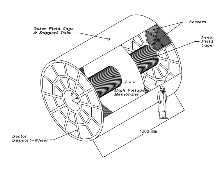
Figure 1: The STAR TPC surrounds a beam-beam interaction region at RHIC. The collisions take place near the center of the TPC.

Table 1 lists some basic parameters for the STAR TPC. The measured TPC performance has generally agreed with standard codes such as MAGBOLTZ[9] and GARFIELD[10]. Only for the most detailed studies has it been necessary to make custom measurements of the electrostatic or gas parameters (e.g. the drift velocity in the gas).

Item	Dimension	Comment
Length of the TPC	420 cm	Two halves, 210 cm long
Outer Diameter of the Drift Volume	400 cm	200 cm radius
Inner Diameter of the Drift Volume	100 cm	50 cm radius
Distance: Cathode to Ground Plane	209.3 cm	Each side
Cathode	400 cm diameter	At the center of the TPC
Cathode Potential	28 kV	Typical
Drift Gas	P10	10% methane, 90% argon
Pressure	Atmospheric + 2 mbar	Regulated at 2 mbar above Atm.
Drift Velocity	5.45 cm / $\mu$s	Typical
Transverse Diffusion ($\sigma$)	$230\mu m/\sqrt{cm}$	140 V/cm & 0.5 T
Longitudinal Diffusion ($\sigma$)	$360\mu m/\sqrt{cm}$	140 V/cm
Number of Anode Sectors	24	12 per end
Number of Pads	136,608
Signal to Noise Ratio	20 : 1
Electronics Shaping Time	180 ns	FWHM
Signal Dynamic Range	10 bits
Sampling Rate	9.4 MHz
Sampling Depth	512 time buckets	380 time buckets typical
Magnetic Field	0, $\pm 0.25$ T, $\pm 0.5$ T	Solenoidal

Table 1: Basic parameters for the STAR TPC and its associated hardware.

2 Cathode and Field Cage

The uniform electric field in the TPC is defined by establishing the correct boundary conditions with the parallel disks of the central membrane (CM), the end-caps, and the concentric field cage cylinders. The central membrane is operated at 28 kV. The end caps are at ground. The field cage cylinders provide a series of equi-potential rings that divide the space between the central membrane and the anode planes into 182 equally spaced segments. One ring at the center is common to both ends. The central membrane is attached to this ring. The rings are biased by resistor chains of 183 precision 2 M$\Omega$ resistors which provide a uniform gradient between the central membrane and the grounded end caps.

The CM cathode, a disk with a central hole to pass the Inner Field Cage (IFC), is made of 70 $\mu$m thick carbon loaded Kapton film with a surface resistance of 230 $\Omega$ per square. The membrane is constructed from several pie shape Kapton sections bonded with double sided tape. The membrane is secured under tension to an outer support hoop which is mounted inside the Outer Field Cage (OFC) cylinder. There is no mechanical coupling to the IFC other than a single electrical connection. This design minimizes material and maintains a good flat surface to within 0.5 mm.

Thirty six aluminum stripes have been attached to each side of the CM to provide a low work-function material as the target for the TPC laser calibration system[12, 13]. Electrons are photo-ejected when ultraviolet laser photons hit the stripes, and since the position of the narrow stripes are precisely measured, the ejected electrons can be used for spatial calibration.

The field cage cylinders serve the dual purpose of both gas containment and electric field definition. The mechanical design was optimized to reduce mass, minimize track distortions from multiple Coulomb scattering, and reduce background from secondary particle production. Mechanically, the walls of the low mass self supporting cylinders are effectively a bonded sandwich of two metal layers separated by NOMEX[14] honeycomb ( see Fig. 2 for a cutaway view) . The metal layers are in fact flexible PC material, Kapton, with metal on both sides. The metal is etched to form electrically separated 10 mm strips separated by 1.5 mm. The pattern is offset on the two sides of the kapton so that the composite structure behaves mechanically more like a continuous metal sheet. The 1.5 mm break is the minimum required to maintain the required voltage difference between rings safely. This limits the dielectric exposure in the drift volume thus reducing stray, distorting electric fields due to charge build up on the dielectric surfaces. Minimizing the break has the additional benefit of improving the mechanical strength. Punch-through pins were used to electrically connect the layers on the two sides of the sandwich.

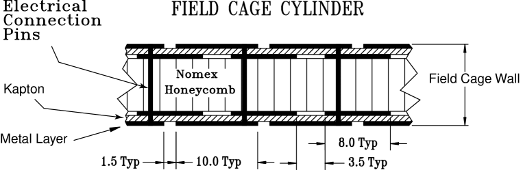
Figure 2: A cutaway view of the inner field cage (IFC) showing the construction and composition of the cylinder wall. Dimensions are in mm.

The lay-up and bonding of the field cage sandwich was done on mandrels constructed of wood covered with rigid foam which was turned to form a good cylindrical surface. Commercially available metal covered Kapton is limited in width to $\approx$20 cm so the lay-up was done with multiple etched metal-Kapton sheets wrapped around the circumference of the mandrel. A laser interferometer optical tool was used to correctly position the sheets maintaining the equi-potential ring alignment to within 50 $\mu$m differentially and better than 500 $\mu$m, overall. The mandrels were constructed with a double rope layer under the foam. The ropes were unwound to release the mandrel from the field cage cylinder at completion of the lay-up.

A summary of the TPC material thicknesses in the tracking volume are presented in Table 2. The design emphasis was to limit material at the inner radius where multiple Coulomb scattering is most important for accurate tracking and accurate momentum reconstruction. For this reason aluminum was used in the IFC, limiting it to only 0.5% radiation length ($X_{0}$). To simplify the construction, and the electrical connections, copper was used for the OFC. Consequently, the OFC is significantly thicker, 1.3% $X_{0}$, but still not much more than the detector gas itself. The sandwich structure of the OFC cylinder wall is 10 mm thick while the IFC has a wall thickness of 12.9 mm.

Nitrogen gas or air insulation was used to electrically isolate the field cage from the surrounding ground structures. This design choice requires more space than solid insulators, but it has two significant advantages. One advantage is to reduce multiple scattering and secondary particle production. The second advantage is the insulator is not vulnerable to permanent damage. The gas insulator design was chosen after extensive tests showed that the field cage kapton structures and resistors could survive sparks with the stored energy of the full size field cage. The IFC gas insulation is air and it is 40 cm thick without any detectors inside the IFC. It is 18 cm thick with the current suite of inner detectors. The OFC has a nitrogen layer 5.7 cm thick isolating it from the outer shell of the TPC structure. The field cage surfaces facing the gas insulators are metallic potential graded structures which are the same as the surfaces facing the TPC drift volume. In addition to the mechanical advantages of a symmetric structure, this design avoids uncontrolled dielectric surfaces where charge migration can lead to local high fields and surface discharges in the gas insulator volume.

The outermost shell of the TPC is a structure that is a sandwich of material with two aluminum skins separated by an aluminum honeycomb. The skins are a multi-layer wraps of aluminum. The construction was done much like the field cage structures using the same cylindrical mandrel. The innermost layer, facing the OFC, is electrically isolated from the rest of the structure and it is used as a monitor of possible corona discharge across the gas insulator. The outer shell structure is completely covered by aluminum extrusion support rails bonded to the surface. The support rails carry the Central Trigger Barrel (CTB) trays. These extrusions have a central water channel for holding the structure at a fixed temperature. This system intercepts heat from external sources, the CTB modules and the magnet coils, which run at a temperature significantly higher than the TPC. This is just one part of the TPC temperature control system which also provides cooling water for the TPC electronics on the end-caps.

Structure	Material	Density($g/cm^{3}$)	$X_{0}$ ($g/cm^{2}$)	Thickness (cm)	Thickness ($\%X_{0}$)
Insulating gas	$N_{2}$	1.25E-03	37.99	40	0.13
TPC IFC	Al	2.700	24.01	0.004	0.04
TPC IFC	Kapton	1.420	40.30	0.015	0.05
TPC IFC	NOMEX	0.064	40	1.27	0.20
TPC IFC	Adhesive	1.20	40	0.08	0.23
IFC Total (w/gas)					0.65

Structure	Material	Density($g/cm^{3}$)	$X_{0}$ ($g/cm^{2}$)	Thickness (cm)	Thickness ($\%X_{0}$)
TPC gas	P10	1.56E-03	20.04	150.00	1.17
TPC OFC	Cu	8.96	12.86	0.013	0.91
TPC OFC	Kapton	1.420	40.30	0.015	0.05
TPC OFC	NOMEX	0.064	40	0.953	0.15
OFC	Adhesive	1.20	40	0.05	0.15
OFC Total (w/gas)					2.43

Table 2: Material thickness for the inner (IFC) and outer (OFC) electrostatic field cages[15] .

3 The TPC End-caps with the Anodes and Pad Planes

The end-cap readout planes of STAR closely match the designs used in other TPCs such as PEP4, ALEPH, EOS and NA49 but with some refinements to accommodate the high track density at RHIC and some other minor modifications to improve reliability and simplify construction. The readout planes, MWPC chambers with pad readout, are modular units mounted on aluminum support wheels. The readout modules, or sectors, are arranged as on a clock with 12 sectors around the circle. The modular design with manageable size sectors simplifies construction and maintenance. The sectors are installed on the inside of the spoked support wheel so that there are only 3 mm spaces between the sectors. This reduces the dead area between the chambers, but it is not hermetic like the more complicated ALEPH TPC design[11]. The simpler non-hermetic design was chosen since it is adequate for the physics in the STAR experiment.

The chambers consist of four components; a pad plane and three wire planes (see Fig. 3). The amplification/readout layer is composed of the anode wire plane of small, 20 $\mu$m, wires with the pad plane on one side and the ground wire plane on the other. The third wire plane is a gating grid which will be discussed later. Before addressing the details of the amplification region, a word about the chosen wire direction. The direction is set to best determine the momentum of the highest transverse momentum ($p_{T}$) particles whose tracks are nearly straight radial lines emanating from the interaction point (the momentum of low $p_{T}$ particles is well determined without special consideration). The sagitta of the high $p_{T}$ tracks is accurately determined by setting the anode wires roughly perpendicular to the straight radial tracks because position resolution is best along the direction of the anode wire. In the other direction, the resolution is limited by the quantized spacing of the wires (4 mm between anode wires). The dimensions of the rectangular pads are likewise optimized to give the best position resolution perpendicular to the stiff tracks. The width of the pad along the wire direction is chosen such that the induced charge from an avalanche point on the wire shares most of it’s signal with only 3 pads. This is to say that the optimum pad width is set by the distance from the anode wire to the pad plane. Concentrating the avalanche signal on 3 pads gives the best centroid reconstruction using either a 3-point gaussian fit or a weighted mean. Accuracy of the centroid determination depends on signal-to-noise ratio and track angle, but it is typically better than 20% of the narrow pad dimension. There are additional tradeoffs dictating details of the pads’ dimensions which will be discussed further in connection with our choice of two different sectors designs, one design for the inner radius where track density is highest and another design covering the outer radius region. Details of the two sector designs can be found in Table 3 and Figure 4.

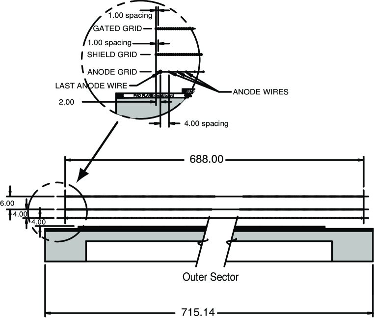
Figure 3: A cutaway view of an outer sub-sector pad plane. The cut is taken along a radial line from the center of the TPC to the outer field cage so the center of the detector is towards the right hand side of the figure. The figures shows the spacing of the anode wires relative to the pad plane, the ground shield grid, and the gated grid. The bubble diagram shows additional detail about the wire spacing. The inner sub-sector pad plane has the same layout except the spacing around the anode plane is 2 mm instead of the 4 mm shown here. All dimensions are in millimeters.

The outer radius sub-sectors have continuous pad coverage to optimize the $dE/dx$ resolution (ie. no space between pad rows). This is optimal because the full track ionization signal is collected and more ionization electrons improve statistics on the $dE/dx$ measurement. Another modest advantage of full pad coverage is an improvement in tracking resolution due to anti-correlation of errors between pad rows. There is an error in position determination for tracks crossing a pad row at an angle due to granularity in the ionization process (Landau fluctuations). If large clusters of ionization occur at the edge of the pad row they pull the measured centroid away from the true track center. But, there is a partially correcting effect in the adjacent pad row. The large clusters at the edge also induce signal on the adjacent pad row producing an oppositely directed error in the measured position in this adjacent row. This effective cross talk across pad rows, while helpful for tracking precision, causes a small reduction in $dE/dx$ resolution.

Item	Inner Subsector	Outer Subsector	Comment
Pad Size	2.85 mm x 11.5 mm	6.20 mm x 19.5 mm
Isolation Gap between pads	0.5 mm	0.5 mm
Pad Rows	13 (#1-#13)	32 (#14-#45)
Number of Pads	1,750	3,942	5,692 total
Anode Wire to Pad Plane Spacing	2 mm	4 mm
Anode Voltage	1,170 V	1,390 V	20:1 signal:noise
Anode Gas Gain	3,770	1,230

Table 3: Comparison of the Inner and Outer subsector geometries.

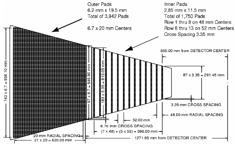
Figure 4: The anode pad plane with one full sector shown. The inner sub-sector is on the right and it has small pads arranged in widely spaced rows. The outer sub-sector is on the left and it is densely packed with larger pads.

On the outer radius sub-sectors the pads are arranged on a rectangular grid with a pitch of 6.7 mm along the wires and 20.0 mm perpendicular to the wires. The grid is phased with the anode wires so that a wire lies over the center of the pads. There is a 0.5 mm isolation gap between pads. The 6.7 mm pitch and the 4 mm distance between the anode wire plane is consistent with the transverse diffusion width of the electron cloud for tracks that drift the full 2 meter distance. More explicitly, with a 4 mm separation between pad plane and anode plane the width of the induced surface charge from a point avalanche is the same as the diffusion width. The pad pitch of 6.7 mm places most of the signal on 3 pads which gives good centroid determination at minimum gas gain. This matching gives good signal to noise without serious compromise to two-track resolution. The pad size in the long direction ( 20.0 mm pitch) was driven by available electronic packaging density and funding, plus the match to longitudinal diffusion. The z projection of 20.0 mm on $\eta$ = 1 tracks matches the longitudinal diffusion spread in z for $\eta$ = 0 tracks drifting the full two meters.

The inner sub sectors are in the region of highest track density and thus are optimized for good two-hit resolution. This design uses smaller pads which are 3.35 mm by 12 mm pitch. The pad plane to anode wire spacing is reduced accordingly to 2 mm to match the induced signal width to  3 pads. The reduction of the induced surface charge width to less than the electron cloud diffusion width improves two track resolution a small amount for stiff tracks $\approx$ perpendicular to the pad rows at $\eta$ $\approx$0. The main improvement in two track resolution, however, is due to shorter pad length (12 mm instead of 20 mm). This is important for lower momentum tracks which cross the pad row at angles far from perpendicular and for tracks with large dip angle. The short pads give shorter projective widths in the r-$\phi$ direction (the direction along the pad row), and the z direction (the drift direction) for these angled tracks. The compromise inherent in the inner radius sub-sector design with smaller pads is the use of separate pad rows instead of continuous pad coverage. This constraint imposed by the available packing density of the front end electronics channels means that the inner sector does not contribute significantly to improving the $dE/dx$ resolution. The inner sector only serves to extend the position measurements along the track to small radii thus improving the momentum resolution and the matching to the inner tracking detectors. An additional benefit is detection of particles with lower momentum.

The design choices, pad sizes, and wire-to-pad spacing, for the two pad plane sector geometries were verified through simulation and testing with computer models [2, 3], but none of the desired attributes: $dE/dx$ resolution, momentum resolution and two track resolution show a dramatic dependence on the design parameters. This is in part due to the large variation in track qualities such as dip angle, drift distance, and crossing angle. While it is not possible with a TPC to focus the design on a particular condition and optimize performance, a lot is gained through over-sampling and averaging. In addition to simulations, prototype pad chambers were built and studied to verify charge-coupling parameters and to test stability at elevated voltages [16].

The anode wire plane has one design feature that is different than in other TPCs. It is a single plane of 20 $\mu$m wires on a 4 mm pitch without intervening field wires. The elimination of intervening field wires improves wire chamber stability and essentially eliminates initial voltage conditioning time. This is because in the traditional design both the field wire and the anode wires are captured in a single epoxy bead. The large potential difference on the field and anode wires places significant demands on the insulating condition of the epoxy surface. The surface is much less of a problem in our design where the epoxy bead supports only one potential. This wire chamber design requires a slightly higher voltage on the anode wires to achieve the same electric field at the anode wire surface (i.e. a higher voltage to achieve the same gas gain) but this is not a limitation on stability. Another small advantage in this design is that we can operate the chambers at a lower gas gain (35% lower for the inner sector) [16] since with this design the readout pads pick-up a larger fraction of the total avalanche signal. Like other TPCs, the edge wires on the anode wire plane are larger diameter to prevent the excess gain that would otherwise develop on the last wire.

Most of the anode wires are equipped with amplifiers and discriminators that are used in the trigger to detect tracks passing through the end cap. The discriminators are active before the electrons drift in from tracks in the drift volume.

Another special feature of the anode plane is a larger than normal (1 nF) capacitor to ground on each wire. This reduces the negative cross talk that is always induced on the pads under a wire whenever an avalanche generates charge anywhere along the wire. The negative cross talk comes from capacitive coupling between the wire and the pad. The AC component of the avalanche charge on a wire capacitively couples to the pads proportionally as $C_{p}/C_{total}$ where $C_{p}$ is the pad-to-wire capacitance and $C_{total}$ is the total capacitance of the wire to ground. In the high track density at RHIC, there can be multiple avalanches on a wire at any time so it is important to minimize this source of cross-talk and noise. The 1 nF grounding capacitor is a compromise between cross talk reduction and wire damage risk. Our tests showed that the stored energy in larger capacitors can damage the wire in the event of a spark.

The gas gain, controlled by the anode wire voltage, has been set independently for the two sector types to maintain a 20:1 signal to noise for pads intercepting the center of tracks that have drifted the full 2 meters. This choice provides minimum gain without significantly impacting the reconstructed position resolution due to electronic noise. The effective gas gain needed to achieve this signal to noise is 3,770 for the inner sector and 1,230 for the outer sector. As discussed in detail in Ref. [17] the required gas gain depends on diffusion size of the electron drift cloud, pad dimensions, amplifier shaping time, the avalanche-to-pad charge-coupling fractions and the electronic noise which for our front end electronics is $\approx$1000 electrons rms.

The ground grid plane of 75 $\mu$m wires completes the sector MWPC. The primary purpose of the ground grid is to terminate the field in the avalanche region and provide additional rf shielding for the pads. This grid can also be pulsed to calibrate the pad electronics. A resistive divider at the grid provides 50 $\Omega$ termination for the grid and and 50 $\Omega$ termination for the pulser driver.

The outermost wire plane on the sector structure is the gating grid located 6 mm from the ground grid. This grid is a shutter to control entry of electrons from the TPC drift volume into the MWPC. It also blocks positive ions produced in the MWPC, keeping them from entering the drift volume where they would distort the drift field. The gating grid plane can have different voltages on every other wire. It is transparent to the drift of electrons while the event is being recorded and closed the rest of the time. The grid is ‘open’ when all of the wires are biased to the same potential (typically 110 V). The grid is ‘closed’ when the voltages alternate $\pm$ 75 V from the nominal value. The positive ions are too slow to escape during the open period and get captured during the closed period. The STAR gating grid design is standard. Its performance is very well described by the usual equations [11]. The gating grid driver has been designed to open and settle rapidly (100 V in 200 ns). Delays in opening the grid shorten the active volume of the TPC because electrons that drift into the grid prior to opening are lost. The combined delay of trigger plus the opening time for the gating grid is 2.1 $\mu$s. This means that the useful length of the active volume is 12 cm less than the physical length of 210 cm. To limit initial data corruption at the opening of the gate, the plus and minus grid driving voltages are well matched in time and amplitude to nearly cancel the induced signal on the pads.

The gating grid establishes the boundary conditions defining the electric field in the TPC drift volume at the ends of the TPC. For this reason the gating wire planes on the inner and outer sub-sectors are aligned on a plane to preserve the uniform drift field. For the same reason the potential on the gating grid planes must be matched to the potential on the field cage cylinders at the intersection point. Aligning the gating grid plane separates the anode wire planes of the two sector types by 2 mm. The difference in drifting electron arrival time for the two cases is taken into account in the time-to-space position calibration. The time difference is the result of both the 2 mm offset and the different field strengths in the vicinity of the anode wires for the two sector types. The electron drift times near the anode plane was both measured and studied with MAGBOLTZ. The field is nearly uniform and constant from the CM to within 2 mm of the gating grid. We simulated the drift of ionization from 2 mm above the gating grid to the anode wires to estimate the difference between the inner and outer sub-sector drift times. These MAGBOLTZ simulations find that the drift from the CM to the outer sub-sectors requires 0.083 $\mu$s longer than from the CM to the inner sub-sectors. Measurement shows a slightly longer average time difference of 0.087 $\mu$s.

The construction of the sectors followed techniques developed for earlier TPCs. The pad planes are constructed of bromine-free G10 printed circuit board material bonded to a single-piece backing structure machined from solid aluminum plate. Specialized tooling was developed so that close tolerances could be achieved with minimum setup time. Pad plane flatness was assured by vacuum locking the pad plane to a flat granite work surface while the aluminum backer is bonded with epoxy to the pad plane. Wire placement is held to high tolerance with fixed combs on granite work tables during the assembly step of capturing the wires in epoxy beads on the sector backer. Mechanical details of the wires are given in Table 4. The final wire-placement error is less than 7 $\mu$m. Pad location along the plane is controlled to better than 100 microns. The sectors were qualified with over-voltage testing and gas-gain uniformity measurements with an ⁵⁵Fe source.

4 Drift Gas

P10 (90% Argon + 10% Methane) is the working gas in the TPC. The gas system (discussed in detail in [8]) circulates the gas in the TPC and maintains purity, reducing electro negative impurities such as oxygen and water which capture drifting electrons. To keep the electron absorption to a few percent, the oxygen is held below 100 parts per million and water less than 10 parts per million.

All materials used in the TPC construction that are exposed to the drift gas were tested for out-gassing of electron capturing contaminants. This was done with a chamber designed to measure electron attenuation by drifting electrons through a 1 meter long gas sample.

The transverse diffusion[9] in P10 is $230\mu m/\sqrt{\rm cm}$ at 0.5 T or about $\sigma_{T}$ = 3.3 mm after drifting 210 cm. This sets the scale for the wire chamber readout system in the X,Y plane. Similarly, the longitudinal diffusion of a cluster of electrons that drifts the full length of the TPC is $\sigma_{L}$ = 5.2 mm. At a drift velocity of 5.45 cm/$\mu$s, the longitudinal diffusion width is equal to a spread in the drift time of about 230 ns FWHM. This diffusion width sets the scale for the resolution of the tracking system in the drift direction and we have chosen the front-end pad amplifier shaping time and the electronic sampling time accordingly. The shaping time is 180 ns FWHM and the electronic sampling time is 9.4 MHz.

Wire	Diameter	Pitch	Composition	Tension
Anodes	$20\ \mu$m	4 mm	Au-plated W	0.50 N
Anodes - Last wire	125 $\mu$m	4 mm	Au-plated Be-Cu	0.50 N
Ground Plane	$75\ \mu$m	1 mm	Au-plated Be-Cu	1.20 N
Gating Grid	$75\ \mu$m	1 mm	Au-plated Be-Cu	1.20 N

Table 4: Properties of the wires in the readout chambers.

5 Performance of the TPC

This section will discuss the TPC performance using data taken in the RHIC beam in the 2000/2001 run cycle. The TPC performance with cosmic rays without magnetic field has been previously presented[18]. In 2000, the magnetic field was 0.25 T; in 2001 the field was raised to 0.5 T. The TPC performance is strongly affected by the magnetic field because, for example, the transverse diffusion of the electrons that drift through the gas is smaller in higher fields.

The track of an infinite-momentum particle passing through the TPC at mid-rapidity is sampled by 45 pad rows, but a finite momentum track may not cross all 45 rows. It depends on the radius of curvature of the track, the track pseudorapidity, fiducial cuts near sector boundaries, and other details about the particle’s trajectory. While the wire chambers are sensitive to almost 100% of the secondary electrons arriving at the end-cap, the overall tracking efficiency is lower (80-90%) due to the fiducial cuts, track merging, and to lesser extent bad pads and dead channels. There are at most a few percent dead channels in any one run cycle.

The track of a primary particle passing through the TPC is reconstructed by finding ionization clusters along the track. The clusters are found separately in $x,y$ and in $z$ space. (The local $x$ axis is along the direction of the pad row, while the local $y$ axis extends from the beamline outward through the middle of, and perpendicular to, the pad rows. The $z$ axis lies along the beam line.) For example, the $x$-position cluster finder looks for ionization on adjacent pads, within a pad row, but with comparable drift times. And, for simple clusters, the energy from all pads is summed to give the total ionization in the cluster. If two tracks are too close together, the ionization clusters will overlap. These complex clusters are split using an algorithm that looks for peaks with a valley between them and then the ionization is divided between the two tracks. These merged clusters are used only for tracking and not for $dE/dx$ determination because of the uncertainty in the partitioning between the tracks. In central Au-Au events at 200 GeV, about 30% of the clusters are overlapping.

5.1 Reconstruction of the $x$, $y$ position

The $x$ and $y$ coordinates of a cluster are determined by the charge measured on adjacent pads in a single pad row. Assuming that the signal distribution on the pads (pad response function) is Gaussian, the local $x$ is given by a fit, where $h_{1}$, $h_{2}$ and $h_{3}$ are the amplitudes on 3 adjacent pads, with pad $h_{2}$ centered at $y=0$:

$$x={\sigma^{2}\over 2w}\ln{\big{(}{h_{3}\over h_{1}}\big{)}}$$ (1)

where the width of the signal, $\sigma$, is given by

$$\sigma^{2}={w^{2}\over\ln{(h_{2}^{2}/h_{1}h_{3})}}$$ (2)

and $w$ is the pad width. The position uncertainty due to electronics noise may be fairly easily computed in this approach:

$$\Delta x={\Delta h\over h_{c}}{\sigma^{2}\over 2w}\sqrt{\big{(}1-{2x\over w}\big{)}^{2}\exp{\big{(}{-(x+w)^{2}\over\sigma^{2}}\big{)}}+{16x^{2}\over w^{2}}\exp{\big{(}-{x^{2}\over w^{2}}\big{)}}+\big{(}1+{2x\over w}\big{)}^{2}\exp{\big{(}{-(x-w)^{2}\over\sigma^{2}}\big{)}}}$$ (3)

Here $\Delta h$ is the noise, $h_{c}$ is the signal amplitude under a centerd pad ($h_{c}=0$), and the three terms in the root correspond to the the errors on $h_{1}$, $h_{2}$, and $h_{3}$ respectively. For $\Delta h<0.05h$ (a 20:1 signal to noise ratio), the noise contribution is small. The total signal is summed over all above-threshold time buckets. This equation is slightly different from the results in Ref. [19] because it includes the error in the $\sigma$ determination.

The Gaussian approximation has some short-comings. First, it does not exactly match onto the tails the true pad response function which introduces an $x-$dependent bias of a few hundred $\mu$m. More importantly, the algorithm deteriorates at large crossing angles. When a track crosses the pad row at large angles, it deposits ionization on many pads and any 3 adjacent pads will have similar amplitude signals. In this case, a weighted mean algorithm, using all of the pads above a certain threshold is much more effective.

Figures 5a and 5c show the position resolution along the pad rows (local $x$) for both field settings of the magnet. The sigma is extracted by fitting a Gaussian to the residual distribution, i.e. the distance between the hit position and the track extrapolation.

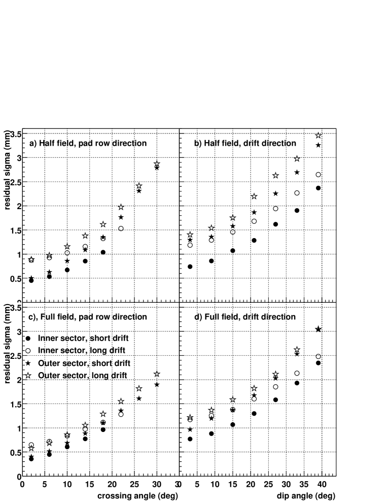
Figure 5: Position resolution across the pad rows and along the $z$ axis of the TPC. The crossing angle is the angle between the particle momentum and the pad row direction. The dip angle is the angle between the particle momentum and the drift direction, $\theta=\cos^{-1}{(p_{z}/p)}$.

5.2 Reconstruction of the $z$ position in the TPC

The $z$ coordinate of a point inside the TPC is determined by measuring the time of drift of a cluster of secondary electrons from the point of origin to the anodes on the endcap and dividing by the average drift velocity. The arrival time of the cluster is calculated by measuring the time of arrival of the electrons in “time buckets” and weighting the average by the amount of charge collected in each bucket. (Each time bucket is approximately 100 nsec long.) The signal from a typical cluster covers several time buckets because of three phenomena: the longitudinal diffusion of the drifting electrons, the shaping of the signal by the preamplifier electronics, and the track dip angle. The preamplifier shaping time is chosen to correspond to the size of the electron cloud for particles drifting and diffusing the entire length of the TPC[20]. This setting smooths out the random fluctuations of the average cluster positions introduced by statistics and diffusion. The amplifier also has cancellation circuitry to remove the long current tail characteristic of MWPCs[21].

The length of the signal reaching a pad depends on the dip angle, $\theta$, which is the angle between the particle momentum and the drift direction. The ionization electrons are spread over a distance $d$ along the beam axis, with $d=L/\tan(\theta)$ and $L$ is the length of the pad.

The drift velocity for the electrons in the gas must be known with a precision of 0.1% in order to convert the measured time into a position with sufficient accuracy. But the drift velocity will change with atmospheric pressure because the TPC is regulated and fixed at 2 mbar above atmospheric pressure. Velocity changes can also occur from small changes in gas compositon. We minimize the effect of these variations in two ways. First, we set the cathode voltage so the electric field in the TPC corresponds to the peak in the drift velocity curve (i.e. velocity vs. electric field / pressure). The peak is broad and flat and small pressure changes do not have a large effect on the drift velocity at the peak. Second, we measure the drift velocity independently every few hours using artificial tracks created by lasers beams[12, 13]. Table 1 gives the typical drift velocities and cathode potentials.

The conversion from time to position also depends on the timing of the first time bucket with respect to the collision time. This time offset has several origins: trigger delay, the time spent by the electron drifting from the gating grid to the anode wires, and shaping of the signal in the front end electronics. The delay is constant over the full volume of the TPC and so the timing offset can be adjusted, together with the drift velocity, by reconstructing the interaction vertex using data from one side of the TPC only and later matching it to the vertex found with data from the other side of the TPC. Local variations of the time offset can appear due to differences between different electronic channels and differences in geometry between the inner and outer sector pad planes. These electronic variations are measured and corrected for by applying a calibrated pulse on the ground plane. Fluctuations on the order of 0.2 time buckets are observed between different channels.

Figures 5b and 5d show the position resolution along the $z$ axis of the TPC in 0.25T and 0.5T magnetic fields, respectively. The resolution is best for short drift distances and small dip angles. The position resolution depends on the drift distance but the dependence is weak because of the large shaping time in the electronics, which when multiplied by the drift velocity ($\approx 1$ cm), is comparable to or greater than the longitudinal diffusion width ($\approx 0.5$ cm). The position resolution for the two magnetic field settings is similar. The resolution deteriorates, however, with increasing dip angle because the length of path received by a pad is greater than the shaping time of the electronics (times drift velocity) and the ionization fluctuations along the particle path are not fully integrated out of the problem.

5.3 Distortions

The position of a secondary electron at the pad plane can be distorted by non-uniformities and global misalignments in the electric and magnetic fields of the TPC. The non-uniformities in the fields lead to a non-uniform drift of the electrons from the point of origin to the pad plane. In the STAR TPC, the electric and magnetic fields are parallel and nearly uniform in $r$ and $z$. The deviations from these ideal conditions are small and a typical distortion along the pad row is $\leq$ 1 mm before applying corrections.

Millimeter-scale distortions in the direction transverse to the path of a particle, however, are important because they affect the transverse momentum determination for particles at high $p_{T}$. In order to understand these distortions, and correct for them, the magnetic field was carefully mapped with Hall probes and an NMR probe before the TPC was installed in the magnet[7]. It was not possible to measure the electric fields and so we calculated them from the known geometry of the TPC. With the fields known, we correct the hit positions along the pad rows using the distortion equations for nearly parallel electric and magnetic fields[11].

$$\delta_{x}=\int{-\omega\tau{B}_{y}+\omega^{2}\tau^{2}{B}_{x}\over(1+\omega^{2}\tau^{2}){B}_{z}}dz+\int{{E}_{x}+\omega\tau{E}_{y}\over(1+\omega^{2}\tau^{2}){E}_{z}}dz$$ (4)

$$\delta_{y}=\int{\omega\tau{B}_{x}+\omega^{2}\tau^{2}{B}_{y}\over(1+\omega^{2}\tau^{2}){B}_{z}}dz+\int{{E}_{y}-\omega\tau{E}_{x}\over(1+\omega^{2}\tau^{2}){E}_{z}}dz$$ (5)

where $\delta_{x}$ is the distortion in the $x$ direction, $\vec{E}$ and $\vec{B}$ are the electric and magnetic fields, $\omega$ is the signed cyclotron frequency, and $\tau$ is the characteristic time between collisions as the electron diffuses through the gas.

These are precisely the equations in Blum and Rolandi[11], except that they are valid for any $\vec{E}$ field or $\vec{B}$ field configuration while the equations in Blum and Rolandi are not valid for all orientations of $\vec{E}$ and $\vec{B}$. Our equations differ from Blum and Rolandi in the definition of $\omega\tau$. In Blum and Rolandi, $\omega\tau$ is always positive. Here, $\omega\tau$ is signed, with the sign depending on the directions of ${B}_{z}$, ${E}_{z}$ and the drift velocity ${u}_{z}$:

$$\omega\tau=k{{u}_{z}(cm/\mu s)\over{E}_{z}(V/cm)}{B}_{z}(T)$$ (6)

where $k$ is a constant. The negative charge of the drifting electrons is included in the sign of $u_{z}$. For example, the STAR electric field always points towards the central membrane and electrons always drift away from it, while $B_{z}$ can point in either direction. Here, $k\approx 100$ and it depends on microscopic physics that is not represented in equations 4 and 5. For precise work, $k$ must be determined by measuring $\omega\tau$ directly[11, 22]. In STAR, $k=110$ and so $|\omega\tau|=1.15$ at 0.25 T, rising to $|\omega\tau|=2.30$ at 0.5 T. The magnitude of the distortion corrections are given in Table 5.

Figure 6 shows the sum of the distortion corrections as a function of radius and $z$ inside the active volume of the TPC. With these distortion corrections applied, the relative error between a point and the track-model fit is 50 $\mu$m while the absolute error for any one point is about 500 $\mu$m.

Cause of the Distortion	Magnitude of the Imperfection	Magnitude of the Correction
Non-uniform B field	$\pm 0.0040$ T	0.10 cm
Geometrical effect between the inner and outer sub-sectors	Exact calculation based on geometry	0.05 cm (near pad row 13)
Cathode - non-flat shape and tilt	0.1 cm	0.04 cm
The angular offset between E and B field	0.2 mr	0.03 cm
TPC endcaps - non-flat shape and tilt	0.1 cm	0.03 cm
Misalignment between IFC and OFC	0.1 cm	0.03 cm
Space Charge build up in the TPC	0.001 C / $\epsilon_{0}$	0.03 cm average over volume

Table 5: The distortion corrections applied to STAR data; their cause, and the magnitude of their effect on the data.

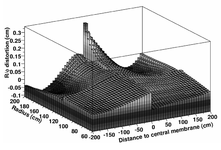
Figure 6: The sum of all distortion corrections. The sum includes the distortions caused by the magnetic field non-uniformities, misalignment between the axis of the magnetic and electric fields, the effects of a tilted central membrane, non-flat end-caps, and local electric field imperfections at the junction of the inner and outer sectors at $R\approx 120$ cm.

5.4 Two hit resolution

The inner and outer sub-sectors have different size pads and so their two-hit resolutions are different. Figure 7 shows the efficiency of finding two hits as a function of the distance separating them. The efficiency depends on whether the track segment is observed in the inner or the outer sub-sectors. The efficiency is the ratio of the distributions of the distance separating 2 hits from the same event and 2 hits from different events. Two hits can be completely resolved when they are separated in the padrow direction (i.e. along the local $x$ axis) by at least 0.8 cm in the inner sector and 1.3 cm in the outer sector. Similarly, two hits are completely resolved when they are separated in the drift direction (i.e. along the $z$ axis) by 2.7 cm in the inner sector and 3.2 cm in the outer sector.

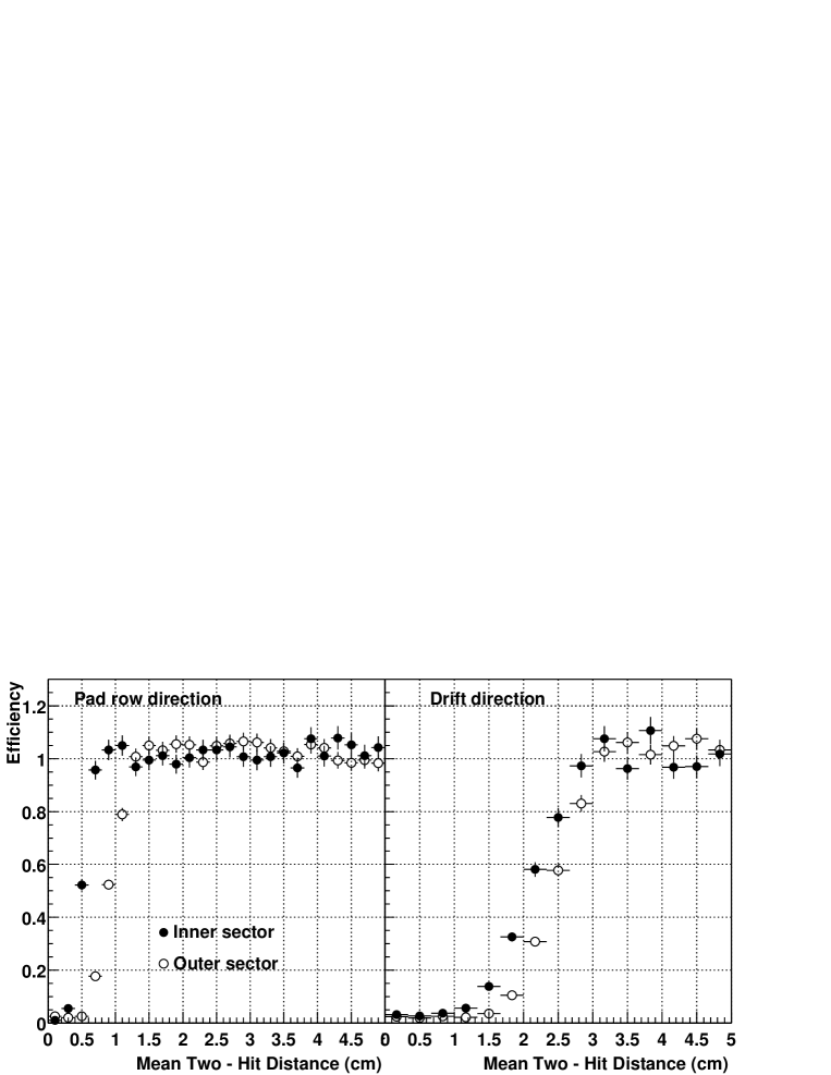
Figure 7: Two-hit resolution in the STAR TPC. The drift direction is along the $z$ axis and the pad row direction is along the local $x$ axis.

5.5 Tracking Efficiency

The tracking software performs two distinct tasks. First, the algorithms associate space points to form tracks and, second, they fit the points on a track with a track-model to extract information such as the momentum of the particle. The track-model is, to first order, a helix. Second order effects include the energy lost in the gas which causes a particle trajectory to deviate slightly from the helix. In this section, we will discuss the efficiency of finding tracks with the software.

The tracking efficiency depends on the acceptance of the detector, the electronics detection efficiency, as well as the two-hit separation capability of the system. The acceptance of the TPC is 96% for high momentum tracks traveling perpendicular the beamline. The 4% inefficiency is caused by the spaces between the sectors which are required to mount the wires on the sectors. The software also ignores any space points that fall on the last 2 pads of a pad row. This fiducial cut is applied to avoid position errors that result from tracks not having symmetric pad coverage on both sides of the track. It also avoids possible local distortions in the drift field. This fiducial cut reduces the total acceptance to 94%.

The detection efficiency of the electronics is essentially 100% except for dead channels and the dead channel count is usually below 1% of the total. However, the system cannot always separate one hit from two hits on adjacent pads and this merging of hits reduces the tracking efficiency. The software also applies cuts to the data. For example, a track is required to have hits on at least 10 pad rows because shorter tracks are too likely to be broken track fragments. But this cut can also remove tracks traveling at a small angle with respect to the beamline and low momentum particles that curl up in the magnetic field. Since the merging and minimum pad rows effects are non-linear, we can’t do a simple calculation to estimate their effects on the data. We can simulate them, however.

In order to estimate the tracking efficiency, we embed simulated tracks inside real events and then count the number of simulated tracks that are in the data after the track reconstruction software has done its job. The technique allows us to account for detector effects and especially the losses related to a high density of tracks. The simulated tracks are very similar to the real tracks and the simulator tries to take into account all the processes that lead to the detection of particles including: ionization, electron drift, gas gain, signal collection, electronic amplification, electronic noise, and dead channels. The results of the embedding studies indicate that the systematic error on the tracking efficiency is about 6%.

Figure 8 shows the pion reconstruction efficiency in Au+Au collisions with different multiplicities as a function of the transverse momentum of the primary particle[23]. In high multiplicity events it reaches a plateau of 80% for high $p_{T}$ particles. Below 300 MeV/c the efficiency drops rapidly because the primary particles spiral up inside the TPC and don’t reach the outer field cage. In addition, these low momentum particles interact with the beam pipe and the inner field cage before entering the tracking volume of the TPC. As a function of mulitplicity, the efficiency goes up to the geometrical limit, minus software cuts, for low multiplicity events.

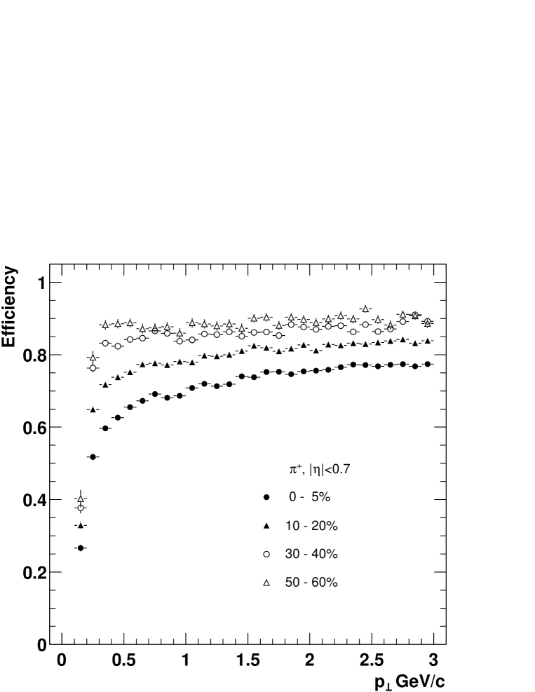
Figure 8: The pion tracking efficiency in STAR for central Au+Au events at RHIC. Tracks with $|y|<0.7$ were used to generate the figure and the magnetic field was set to 0.25 T. The data are binned by centrality. The most central collisions are the the highest multiplicity data and they are shown as black dots. The lowest multiplicity data are shown as open triangles.

5.6 Vertex resolution

The primary vertex can used to improve the momentum resolution of the tracks and the secondary vertices can be separated from the primary vertices if the vertex resolution is good enough. Many of the strange particles produced in heavy ion collisions can be identified this way.

The primary vertex is found by considering all of the tracks reconstructed in the TPC and then extrapolating them back to the origin. The global average is the vertex position. The primary vertex resolution is shown in Fig. 9. It is calculated by comparing the position of the vertices that are reconstructed using each side of the TPC, separately. As expected, the resolution decreases as the square root of the number of tracks used in the calculation. A resolution of 350 $\mu$m is achieved when there are more than 1,000 tracks.

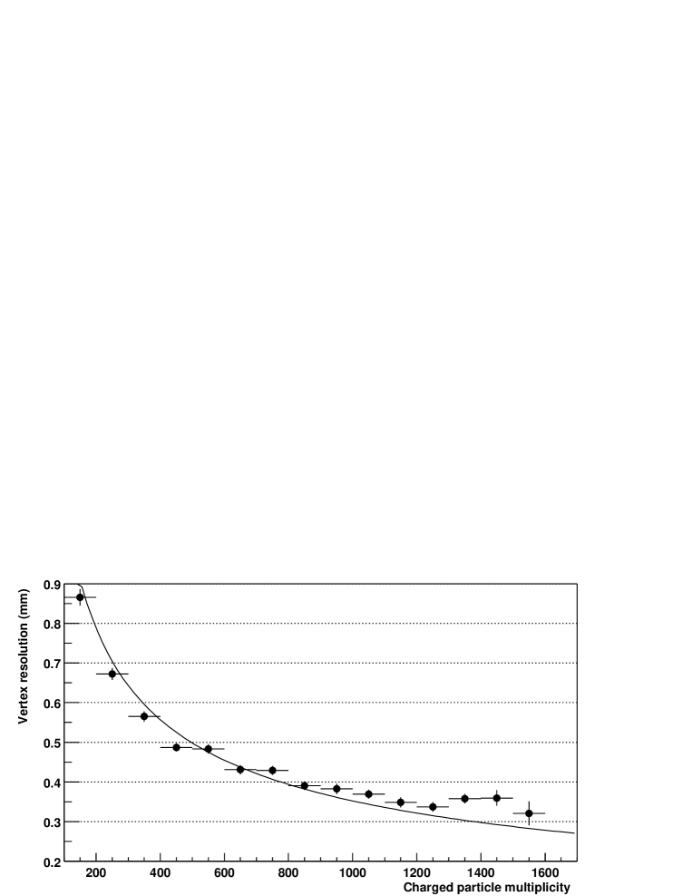
Figure 9: Primary vertex resolution in the transverse plane.

5.7 Momentum resolution

The transverse momentum, $p_{T}$, of a track is determined by fitting a circle through the $x$, $y$ coordinates of the vertex and the points along the track. The total momentum is calculated using this radius of curvature and the angle that the track makes with respect to the $z$ axis of the TPC. This procedure works for all primary particles coming from the vertex, but for secondary decays, such as $\Lambda$ or $K_{s}$, the circle fit must be done without reference to the primary vertex.

In order to estimate the momentum resolution we use the embedding technique discussed above. The track simulator was used to create a track with a known momentum. The track was then embedded in a real event in order to simulate the momentum smearing effects of working in a high track density environment. Figure 10 shows the $p_{T}$ resolution for $\pi^{-}$ and anti-protons in STAR. The figure shows two regimes: at low momentum, where multiple Coulomb scattering dominates (i.e. $p_{T}<400MeV/c$ for pions, and $p_{T}<800$ MeV/c for anti-protons), and at higher momentum where the momentum resolution is limited by the strength of the magnet field and the TPC spatial resolution. The best relative momentum resolution falls between these two extremes and it is 2% for pions.

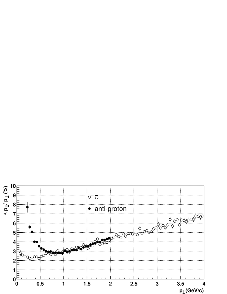
Figure 10: Transverse momentum resolution of the STAR TPC for $\pi^{-}$ and anti-protons in the 0.25 T magnetic field. Tracks are required to be formed by more than 15 hits. Tracks are embedded in minimum bias events. The momentum resolution is calculated as the Gaussian $sigma$.

5.8 Particle identification using $dE/dx$

Energy lost in the TPC gas is a valuable tool for identifying particle species. It works especially well for low momentum particles but as the particle energy rises, the energy loss becomes less mass-dependent and it is hard to separate particles with velocities $v>0.7$c. STAR was designed to be able to separate pions and protons up to 1.2 GeV/c. This requires a relative $dE/dx$ resolution of 7%. The challenge, then, is to calibrate the TPC and understand the signal and gain variations well enough to be able to achieve this goal.

The measured $dE/dx$ resolution depends on the gas gain which itself depends on the pressure in the TPC. Since the TPC is kept at a constant 2 mbar above atmospheric pressure, the TPC pressure varies with time. We monitor the gas gain with a wire chamber that operates in the TPC gas return line. It measures the gain from an ⁵⁵Fe source. It will be used to calibrate the 2001 data, but for the 2000 run, this chamber was not installed and so we monitored the gain by averaging the signal for tracks over the entire volume of the detector and we have done a relative calibration on each sector based on the global average. Local gas gain variations are calibrated by calculating the average signal measured on one row of pads on the pad-plane and assuming that all pad-rows measure the same signal. The correction is done on the pad-row level because the anode wires lie on top of, and run the full length of, the pad-rows.

The read-out electronics also introduce uncertainties in the $dE/dx$ signals. There are small variations between pads, and groups of pads, due to the different response of each readout board. These variations are monitored by pulsing the ground plane of the anode and pad plane read-out system and then assuming that the response will be the same on every pad.

The $dE/dx$ is extracted from the energy loss measured on up to 45 padrows. The length over which the particle energy loss is measured (pad length modulo the crossing and dip angles) is too short to average out ionizations fluctuations. Indeed, particles lose energy going through the gas in frequent collisions with atoms where a few tens of eV are released, as well as, rare collisions where hundreds of eV are released [24]. Thus, it is not possible to accurately measure the average $dE/dx$. Instead, the most probable energy loss is measured. We do this by removing the largest ionization clusters. The truncated mean, where a given fraction (typically 30%) of the clusters having the largest signal are removed, is an efficient tool to measure the most probable $dE/dx$. However, fitting the $dE/dx$ distribution including all clusters associated with a given track was found to be more effective. It also allows us to account for the variation of the most probable energy loss with the length of the ionization samples ($dx$) [25].

Figure 11 shows the energy loss for particles in the TPC as a function of the particle momentum. The data have been corrected for signal and gain variations and the data are plotted using a 70% truncated mean. The magnetic field setting is 0.25 T. The resolution is 8% for a track that crosses 40 pad-rows. At 0.5 T, the $dE/dx$ resolution improves because the transverse diffusion is smaller and this improves the signal to noise ratio for each cluster. Figure 11 includes both primary and secondary particles. The prominent proton, deuteron, and muon bands come from secondary interactions in the beam pipe and IFC, and from pion and kaon decays. Pions and protons can be separated from each other up to 1 GeV/c.

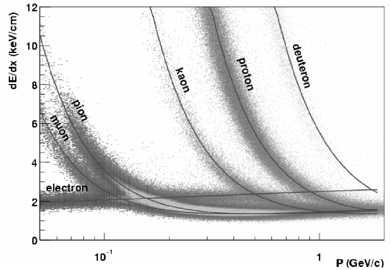
Figure 11: The energy loss distribution for primary and seconday particles in the STAR TPC as a function of the $p_{T}$ of the primary particle. The magnetic field was 0.25 T.

6 Conclusions

The STAR TPC is up and running at RHIC. The detector finished its second year of operation on January 25th, 2002 and the operation of the TPC was stable and reliable throughout both run cycles. Its performance is very close to the original design requirements in terms of tracking efficiency, momentum resolution, and energy loss measurements. Many results from the 2000/2001 data have already been published and they demonstrate that the physics at RHIC is exciting and rich. We invite you to examine these papers[26, 27, 28, 29, 30, 31, 32].

7 Acknowledgements

We wish to thank the RHIC Operations Group and the RHIC Computing Facility at Brookhaven National Laboratory, and the National Energy Research Scientific Computing Center at Lawrence Berkeley National Laboratory for their support. This work was supported by the Division of Nuclear Physics and the Division of High Energy Physics of the Office of Science of the U.S. Department of Energy, the United States National Science Foundation, the Bundesministerium fuer Bildung und Forschung of Germany, the Institut National de la Physique Nucleaire et de la Physique des Particules of France, the United Kingdom Engineering and Physical Sciences Research Council, Fundacao de Amparo a Pesquisa do Estado de Sao Paulo, Brazil, the Russian Ministry of Science and Technology, the Ministry of Education of China, the National Natural Science Foundation of China, and the Swedish National Science Foundation.

References

- [1]
- [2] The STAR Collaboration, The STAR Conceptual Design Report, June 15, 1992 LBL-PUB-5347.
- [3] The STAR Collaboration, STAR Project CDR Update, Jan. 1993 LBL-PUB-5347 Rev.
- [4] http://www.star.bnl.gov and references therein. See especially www.star.bnl.gov Group Documents TPC Hardware.
- [5] H. Wieman et al., IEEE Trans. Nuc. Sci. 44, 671 (1997).
- [6] J. Thomas et al., Nucl. Instum & Meth. A478, 166 (2002).
- [7] F. Bergsma et al., “The STAR Magnet System”, this volume.
- [8] L. Kotchenda et al., “The STAR TPC Gas System”, this volume.
- [9] MAGBOLTZ, a computer program written by S.F. Biagi, Nucl. Instrum & Meth. A421, 234 (1999).
- [10] GARFIELD, a computer program written by R. Veenhof, “A drift chamber simulation program”, CERN Program Library, 1998.
- [11] W. Blum and L. Rolandi, Particle Detection with Drift Chambers, Springer-Verlag, (1993).
- [12] A. Lebedev et al., “The STAR Laser System”, this volume.
- [13] A. Lebedev, Nucl. Instrum & Meth. A478, 163 (2002).
- [14] Nomex, manufactured by Dupont.
- [15] Adhesive is only an estimate.
- [16] W. Betts et al., “Studies of Several Wire and Pad geometries for the STAR TPC”, STAR Note 263, 1996.
- [17] M. Anderson et al., “A Readout System for the STAR Time Projection Chamber”, this volume.
- [18] W. Betts et al., IEEE Trans. Nucl. Sci. 44, 592 (1997).
- [19] G. Lynch, “Thoughts on extracting information from pad data in the TPC,” PEP4 Note TPC-LBL-78-17. April 18, 1978 (unpublished).
- [20] S. Klein et al., IEEE Trans. Nucl. Sci. 43, 1768 (1996).
- [21] E. Beuville et al., IEEE Trans. Nucl. Sci. 43, 1619 (1996).
- [22] S. R. Amendolia et al., Nucl. Instrum. & Meth. A235, 296 (1985).
- [23] Manuel Calderon de la Barca Sanchez, “Charged Hadron Spectra in Au+Au Collisions at 130 GeV”, Ph.D. Thesis, Yale University, December 2001.
- [24] H. Bichsel, “Energy loss in thin layers of argon”, STAR Note 418, http://www.star.bnl.gov/star/starlib/doc/www/sno/ice/sn0418.html
- [25] H. Bichsel, “Comparison of Bethe-Bloch and Bichsel Functions”, STAR Note 439, http://www.star.bnl.gov/star/starlib/doc/www/sno/ice/sn0439.html
- [26] K.H. Ackermann et al., Phys. Rev. Lett. 86, 402 (2001).
- [27] C. Adler et al., Phys. Rev. Lett. 86 4778 (2001).
- [28] C. Adler et al., Phys. Rev. Lett. 87, 082301 (2001).
- [29] C. Adler et al., Phys. Rev. Lett. 87, 112303 (2001).
- [30] C. Adler et al., Phys. Rev. Lett. 87, 182301 (2001).
- [31] C. Adler et al., Phys. Rev. Lett. 87, 262301-1 (2001).
- [32] C. Adler et al., Phys. Rev. Lett. 89, 202301 (2002).