The Muon Anomalous Magnetic Moment and the Standard Model

Abstract

The muon anomalous magnetic moment measurement, when compared with theory, can be used to test many extensions to the standard model. The most recent measurement made by the Brookhaven E821 Collaboration reduces the uncertainty on the world average of $a_{\mu}$ to $0.7$ ppm, comparable in precision to theory. This paper describes the experiment and the current theoretical efforts to establish a correct standard model reference value for the muon anomaly.

1 INTRODUCTION

A precision measurement of the muon anomalous magnetic moment, $a_{\mu}~{}=(g-2)/2$, tests the standard model to the extent that both theory and experiment are well understood. The BNL E821 experiment has steadily increased the precision with which $a_{\mu}$ is known [1, 2, 3, 4]. The result, published [4] in August 2002 dominates the new world average of $a_{\mu}(exp)~{}=~{}11~{}659~{}203(8)\times 10^{-10}$ (0.7 ppm). This includes the complete analysis of all of the positive muon data obtained to date by the E821 group. Another (somewhat smaller) sample of negative muon data is presently being analyzed, and a final run to complete the experiment is planned. Figure 1 illustrates the progression of precision in the measurements of $a_{\mu}$ including the CERN-III [5] and present BNL results.

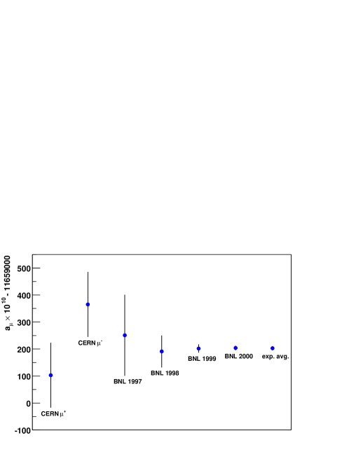
Figure 1: Progression of precision in the measurement of the muon anomalous magnetic moment. The current world average has an uncertainty of 0.7 ppm. Refs. [5, 1, 2, 3, 4]

The standard model (SM) expectation for $a_{\mu}$  is based on QED, the weak interaction, and hadronic loops. All must be computed at the sub-ppm level in order to be compared meaningfully with experiment. Of these contributions, both the QED and weak terms are believed to be known to sufficient precision (see Czarnecki and Marciano [6]), even withstanding a recent examination of eighth-order QED terms, which uncovered a negligible mistake [7], and considerations of hadronic contributions to higher-order weak terms [8]. The need to consider such subtle contributions has reached increased importance because the BNL experimental precision is better than 1 ppm, additional data is being analyzed, and Collaboration discussions have begun to consider an even more precise experiment, either at BNL or the JHF. Many standard model extensions manifest themselves in additional contributions to $a_{\mu}$ at the ppm level, so the relevance of the current studies, in advance of the LHC direct-discovery potential, is quite important.

This paper briefly summarizes the experiment, the analysis of the 2000 data, and the up-to-date theory (i.e., through Nov. 2002). The reader is strongly encouraged to consult the original published papers where appropriate.

1.1 Principle of the Experiment

The experiment measures directly $(g-2)$  and not $g$, where $(g-2)/2$ is approximately $\alpha/2\pi\approx 1/860$. The muon anomaly is determined from the difference between the cyclotron and spin precession frequencies for muons contained in a magnetic storage ring, namely

$$\vec{\omega}_{a}=-{e\over m}\left[a_{\mu}\vec{B}-\left(a_{\mu}-{1\over\gamma^{2}-1}\right)\vec{\beta}\times\vec{E}\right].$$ (1)

Because electric quadrupoles are used to provide vertical focussing in the storage ring, the $\vec{\beta}\times\vec{E}$ term is necessary and illustrates the sensitivity of the spin motion to a radial electric field. This term conveniently vanishes for the “magic” momentum of 3.094 GeV/$c$ when $\gamma=29.3$. The experiment is therefore built around the principle of production and storage of muons centered at this momentum in order to minimize the electric field effect. Because of the finite momentum spread of the stored muons, a 0.3 ppm correction to the observed precession frequency is made to account for the muons above or below the magic momentum. Vertical betatron oscillations induced by the focussing electric field imply that the plane of the muon precession has a time-dependent pitch. Accounting for both of these electric-field related effects introduces a $+0.76(3)$ ppm correction to the precession frequency in the 2000 data.

Muons exhibit circular motion in the storage ring and their spins precess until the time of decay ($\gamma\tau_{\mu}\approx 64.4~{}\mu s$). The net spin precession depends on the integrated magnetic field experienced along the path of the muon. Parity violation leads to a preference for the highest-energy decay electrons (in the muon rest frame) to be emitted in the direction of the muon spin. Therefore, a snapshot of the muon spin direction at time $t$ after injection into the storage ring is obtained, again on average, by the selection of decay electrons in the upper part of the Lorentz-boosted Michel spectrum ($E_{max}\approx 3.1$ GeV). The number of electrons above a selected energy threshold is modulated at frequency $\omega_{a}$ with a threshold-dependent asymmetry $A=A(E_{th})$. The decay electron distribution is described by

$$N(t)=N_{0}\exp(-t/\gamma\tau_{\mu})\left[1+A\cos(\mbox{$\omega_{a}$}t+\phi)\right],$$ (2)

where $N_{0}$, the normalization, $A$ and $\phi$ are all dependent on the energy threshold $E_{th}$. For $E_{th}=2.0$ GeV, $A\approx 0.4$.

In summary, the experiment involves the measurement of the time-averaged quantities $\omega_{a}$ and $B$ in Eq. 1. Here $B$ implies the azimuthially-averaged magnetic field, folded with the muon distribution, the latter being determined from the debunching rate of the initial beam burst and from a tracking simulation. The field strength is measured using nuclear magnetic resonance (NMR) in units of the free proton precession frequency, $\omega_{p}$. The muon anomaly is computed from

$$a_{\mu}=\frac{\mbox{$\omega_{a}$}/\mbox{$\omega_{p}$}}{\lambda-\mbox{$\omega_{a}$}/\mbox{$\omega_{p}$}},$$ (3)

where $\lambda$ is the measured [9] magnetic moment ratio $\mu_{\mu}/\mu_{p}=3.183~{}345~{}39(10)$.

Just like in the analysis of our 1999 data, four independent teams evaluated $\omega_{a}$ and two studied $\omega_{p}$. During the analysis period, the $\omega_{a}$ and $\omega_{p}$ teams maintained separate, secret offsets to their measured frequencies. The offsets were removed and $a_{\mu}$ was computed only after all analyses were complete.

2 EXPERIMENT

2.1 Storage Ring and Magnetic Field Measurement

The Brookhaven muon storage ring [10] is a superferric “C”-shaped magnet, 7.11 m in radius, and open on the inside. Three superconducting coils provide a central field of approximately 1.45 T. Passive and active shimming elements have been improved and optimized since the inception of the experiment.

The magnetic field is measured using pulsed NMR on protons in water- or Vaseline-filled probes [11]. The proton precession frequency is proportional to the local field strength and is measured with respect to the same clock system employed in the determination of $\omega_{a}$. The absolute field is, in turn, determined by comparison with a precision measurement of $\omega_{p}$ in a spherical water sample [12] to a relative precision of better than $10^{-7}$. A subset of the 360 “fixed” probes is used to continuously monitor the field during data taking. These probes are embedded in machined grooves in the outer upper and lower plates of the aluminum vacuum chamber and consequently measure the field just outside of the actual storage volume. Constant field strength is maintained using 36 of the probes in a feedback loop with the main magnet power supply.

The determination of the field inside the storage volume is made by use of a unique non-magnetic trolley which can travel in vacuum through the muon storage volume. The trolley carries 17 NMR probes on a grid appropriate to determine the local multipolarity of the field versus azimuth. Trolley field maps are made every few days and take several hours to complete. Figure 2 shows the contours superimposed on a 9 cm diameter circle, which represents the storage aperature.

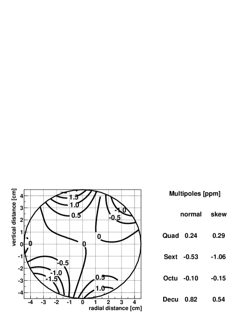
Figure 2: Two-dimensional multipole expansion, averaged over azimuth for the 2000 data-taking period. Half-ppm contours are shown with respect to a central value of 1.451274 T. Multipole amplitudes, relative to this field, are given at the beam aperture.

2.2 Creating and Storing Muons

A highly polarized ($\approx 95\%$) muon sample is created from the decay of 3.15 GeV/$c$ pions in a 72 m long decay channel. The last dipole in this channel is tuned to a momentum approximately 1.7 percent lower than the central pion momentum in order to enhance the muon fraction in the beam, compared to pions, at the entrance to the storage ring. The approximately 1:1 $\pi$ to $\mu$ mix passes through a superconducting inflector magnet [13], which provides a field-free channel in the back of the ring’s iron yoke. A set of three pulsed “kicker” magnets [14] provides a 10 mrad transverse deflection to the muon bunch during the first two turns in the ring and thus places the muons on a central orbit at the magic momentum.

Electric quadrupoles [15] are initially charged asymmetrically to scrape the beam against internal collimaters. After approximately 20 $\mu$s, the voltages are symmetrized at $\pm$24 kV corresponding to a weak-focussing field index $n=0.137$. Coherent horizontal and vertical betatron oscillations (CBO, i.e., oscillations of the beam as a whole), manifest themselves as additional frequencies in the data that must be accommodated (see below). The most important of these is the beating between the cyclotron and the horizontal betatron oscillations, determined as $f_{CBO}=(1-\sqrt{1-n})f_{c}=466$ kHz, where $f_{c}$ is the cyclotron frequency. Note that $f_{CBO}$ is close to twice the precession frequency, $f_{g-2}\approx 229$ kHz, and thus, if ignored, will affect the extraction of $\omega_{a}$. This issue was handled in the 1999 data analysis by accounting for the modulation of the overall rate of events at the horizontal CBO frequency. However, for 2000, $n$ was adjusted slightly, placing $f_{CBO}$ closer to $2f_{g-2}$ compared to 1999. This effect, coupled with significantly higher statistics in 2000, necessitated additional considerations. For example, not only was the overall event rate seen to be modulated, but also the asymmetry and even the phase. The four analyses approached this central problem differently.

2.3 Electron Detection and Pulse Fitting

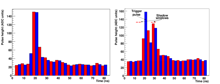
Figure 3: The left panel shows a single pulse on top of a pedestal. The alternating shades illustrate the two independent samples of the WFD. The right panel shows a more complicated pattern, in which two pulses appear close together in time.

The electron detection system consists of 24 lead-scintillating fiber electromagnetic calorimeters [16] located symmetrically around the inside of the storage ring and placed immediately adjacent to the vacuum chamber. The 23 cm long, radially-oriented fiber grid terminates on four lightguides which pipe the light to independent Hamamatsu R1828 2-inch PMTs. The PMT gains are carefully balanced because the four analog signals are added prior to sampling by a dual-phase 400 MHz waveform digitizer. At least 16 digitized samples (usually 24 or more), making “islands,” are recorded for each decay electron event exceeding a hardware threshold of approximately 1 GeV. Two examples of such samples are shown in Fig. 3. The left panel illustrates a simple, single pulse. Offline pulse-finding and fitting techniques are used to establish the electron energy and muon time of decay. Two quasi-independent implementations of an algorithm to extract these quantities formed the basis of two raw-data processing efforts. The methods differ in particular for events which feature multi-pulse pileup, as shown on the right panel in the figure. Here, two pulses are actually sufficiently well-separated that both pulse-finding algorithms can efficiently and accurately determine the correct energies and times (verified by Monte Carlo simulations).

The pulse-finding algorithms also identify the extra events on the tails of the recorded island of samples, which are then used to estimate the time-dependent pileup fraction. These “shadow pulses” are used to construct pileup-only event spectra, which can be subtracted (on average) from the data. This forms a “pileup-free” decay spectrum. Alternatively, the pileup-only spectrum can be fit to determine the parameters necessary to describe the distortion to the uncorrected decay spectrum.

3 ANALYSIS OF $\omega_{a}$

The data set for 2000 consisted of approximately four billion electrons with an energy above 2.0 GeV, recorded $50~{}\mu$s or more after muon injection. These data came from a common set of good runs that avoided known hardware failures, glitches or calibration periods. Data obtained during systematic studies were also removed. The four independent analysis methods then treated the data quite differently after that.

Figure 4: Fourier transform of the residuals from the fit to the data using the simple five-parameter function in Eq. 2.

A fit to the data using the five-parameter function given in Eq. 2 is poor owing to the CBO modulation mentioned above, the deviation from the pure exponential decay due to time-dependent muon losses, and slowly-varying effects such as detector gain or incomplete treatment of pileup. Figure 4 is a Fourier transform of the residuals from such a simple fit. It clearly illustrates the dominant horizontal CBO frequency and its sidebands at $f_{CBO}\pm f_{g-2}$. Note that $f_{g-2}$ has been removed in this representation because of the fit (the frequency is indicated by the dashed line); the small peak at $f_{CBO}-f_{g-2}$ is close to this dashed line and thus potentially interferes with the proper extraction of $f_{g-2}$ or, equivalently, $\omega_{a}$.

Two analysis methods used independent implementations of an expanded conventional functional form applied to a pileup-free electron decay spectrum (pileup events were corrected for as described above). The data were summed for all detectors, which has the effect of reducing the CBO-related amplitudes significantly compared to fits to individual detector spectra. To account for the modulation of the normalization and the asymmetry, $N_{0}\rightarrow N_{0}(t)$ and $A\rightarrow A(t)$ in Eq. 2. The phase was left constant, relying instead on the cancellation of its effect from summing all detectors. The residual effect was included in the systematic uncertainty associated with the overall treatment of CBO.

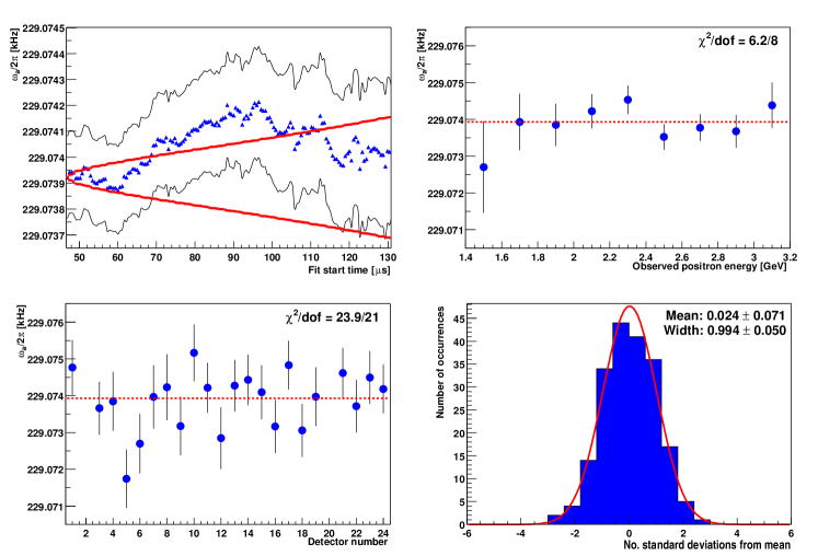
Figure 5: Fit results from the energy-binned analysis versus start time of the fit (upper left), energy bin (upper right), detector station (lower left). The distribution of the 198 individual results with respect to the average is shown in the lower right panel.

A third analysis method started from a spectrum of the data where the exponential decay and other slowly-varying effects are absent, thus isolating the $(g-2)$ oscillation as only identifiable feature. Events are sorted into four sets ($A,B,C,$ and $D$), with sets $A$ and $B$ time shifted by plus or minus one half of a $g-2$ period, respectively, and sets $C$ and $D$ left unaffected. Recombined in the ratio $(A-B)/(C+D)$, this spectrum exhibits an oscillation about zero at frequency $\omega_{a}$. It was then fit using a three-parameter function of the form $r(t)\approx A(E)\sin(\omega_{a}t+\phi_{a}(E))$.

The fourth method divided the data into nine 0.2 GeV wide energy bins for each of the 22 included detectors, resulting in 198 independent data sets. The lowest-energy bin was centered at 1.5 GeV, which meant a significant amount of additional data was considered compared to those analyses described above. The lower-energy threshold also necessitated an extended pileup identification procedure to account for events below twice the hardware threshold. A pileup spectrum was built for each detector and energy bin and fit to extract the amplitude and phase. These parameters were then used in the fit function applied to the data, which was not corrected for pileup, contrary to the other methods. As in the first two methods, a slowly-varying muon loss function was incorporated into the fit. Finally the terms $N_{0},A,$ and $\phi$ in Eq. 2 are permitted to oscillate with the CBO frequency as $1+A(t)_{i}\sin(\omega_{CBO}t+\phi_{i})$, where $A_{i}$ and $\phi_{i}$ are the relative amplitude and phase of the modulation for $N_{0},A,$ and $\phi$. The modulation of these parameters has a time-dependent envelope, which is determined both from independent studies and from the fit itself. Each detector and energy bin was separately fit, with a start time determined from a $\chi^{2}$ stability test.

Figure 5 illustrates the results on $\omega_{a}$ for the fourth method. It shows the fit results versus start time of the fit (upper left), energy bin (upper right), and detector station (lower left). The distribution of the 198 individual results with respect to the average is shown in the bottom right panel. All plots show the expected statistical fluctuations.

3.1 Experimental Results

Summarizing the four methods above involved accounting precisely for data overlap, then combining to form a proper average. Systematics were studied separately for each method. The final result for the 2000 precession frequency is $\omega_{a}/(2\pi)=229~{}074.11(14)(7)$ Hz (0.7  ppm) where the first uncertainty is statistical and the second systematic. Combined with the field value, and weighing with earlier experimental results, the new result for the muon anomaly is $a_{\mu}(exp)=11~{}659~{}203(8)\times 10^{-10}$.

3.2 Update on Theory

The SM prediction for $a_{\mu}$  has gone through several significant changes during the last year; at present there is no single quotable number. The QED [17] and weak contributions [6, 8] are not controversial at the level of relevance required here giving, respectively, $a_{\mu}$(QED)$~{}=~{}11~{}658~{}470.57(0.29)\times 10^{-10}$ (0.025 ppm) and $a_{\mu}$(weak)$~{}=~{}15.1(0.4)\times 10^{-10}$ (0.03 ppm).

The first-order hadronic vacuum polarization (HVP) contribution carries the largest uncertainty in the SM value. It has been updated in 2002 using new $e^{+}e^{-}$ data from Novosibirsk and Beijing and additional hadronic tau decay data from LEP and CLEO. These data are used as input into the dispersion relation to compute $a_{\mu}$(HVP); see Ref. [18]. Davier et al. [19] (DEHZ) recently released an updated evaluation, thus superseding their previous work and the compilations of others (which were sometimes based on preliminary data). The most important finding in DEHZ is that the $e^{+}e^{-}$ and tau-based analyses do not agree with one another. The $e^{+}e^{-}$ evaluation was performed independently [20] confirming the result of DEHZ, but the difference with the tau-based analysis appears to be more fundamental. For example, the $\pi\pi$ spectral functions are not consistent and the difference is shown to be energy dependent. Because the tau input requires invoking CVC and isospin corrections, suspicion first fell to it. These corrections are relatively small [21], and even expanding the uncertainty considerably would not put these data into agreement with the $e^{+}e^{-}$-based result.

Meanwhile, the first reports on a third method to determine HVP using the “radiative return” method have been presented [22]. Fixed center-of-mass energy $e^{+}e^{-}$ collisions are scanned for events having an initial-state radiated photon, thus lowering the effective collision energy. At one accelerator setting, the entire spectral function can be obtained. The reports are preliminary and use only a fraction of the data. However, the procedure looks promising and should be able to confirm or refute the $e^{+}e^{-}$ Novosibirsk result. For now, DEHZ quote $a_{\mu}$(HVP,$e^{+}e^{-}$)$=684.7(7.0)$ or $a_{\mu}$(HVP,tau)$=701.9(6.2)$, both $\times 10^{-10}$ with comparable relative precisions of $\approx 0.6$ ppm. Because the dispersion relation is weighed heavily toward low energies, the true underlying difference in the input data exceeds the relative difference implied to $a_{\mu}$. One should not be tempted to take an average or to ascribe the problem to statistical fluctuations.

Higher-order hadronic contributions [23] give $a_{\mu}$(H-h.o.)$~{}=~{}-10.0(0.6)\times 10^{-10}$. The hadronic light-by-light contribution changed by $200\%$ following Knecht and Nyffeler’s demonstration [24] that this contribution must be positive, contrary to the existing literature [25, 26] by others. Eventually mistakes in earlier work were found [27, 28] and agreement exists on the sign (with confidence), the magnitude (essentially), but not necessarily the uncertainty (see, for example, Ref. [29]). A middle-ground value with a conservative uncertainty is $a_{\mu}$(H-LbL) $=~{}8.6(3.2)\times 10^{-10}$.

Summarizing the above, we obtain the standard model theory to date:

$$~{}~{}~{}a_{\mu}(\rm{SM},e^{+}e^{-}{\rm-based})~{}=~{}11~{}659~{}169.0(7.7)~{}(0.66~{}{\rm ppm)~{}or}$$

$$a_{\mu}({\rm SM,tau-based})~{}=~{}11~{}659~{}186.2(7.0)~{}(0.60~{}{\rm ppm}).$$

Compared to the experiment there is either a 3.0 ($e^{+}e^{-}$) or a 1.6 (tau) standard deviation difference, respectively, leading one to begin to draw very different conclusions (see Fig. 6).

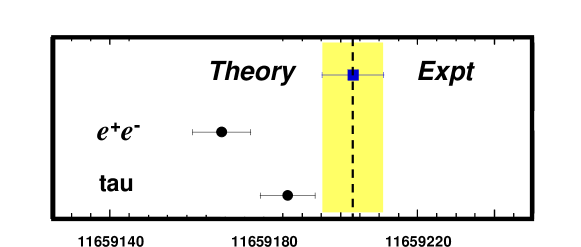
Figure 6: Comparison of experiment with the standard model using either $e^{+}e^{-}$-based or tau-based input for the HVP.

The next year for $(g-2)$ might turn out to be as interesting as the past year: a final data set will be analyzed from negative muons; new input from KLOE and possibly BaBar should resolve the HVP problem; and, finally, we hope to obtain the funds to complete the experiment at BNL and reach the systematic limit of the experiment. Perhaps at that time, we can more meaningfully explore the implications for physics beyond the standard model. At present, the story is clearly still unfolding.

4 Acknowledgments

The $(g-2)$  experiment is supported in part by the U.S. Department of Energy, the U.S. National Science Foundation, the German Bundesminister für Bildung und Forschung, the Russian Minsitry of Science, and the US-Japan Agreement in High Energy Physics. The author thanks his collaborators, and the organizers of PANIC’02 for an excellent meeting.

References

- [1] R.M. Carey et al., Phys. Rev. Lett. 82 (1999) 1632.
- [2] H.N. Brown et al., Muon Collaboration, Phys. Rev. D 62 (2000) 091101.
- [3] H.N. Brown et al., Phys. Rev. Lett. 86 (2001) 2227.
- [4] G.W. Bennett, et al., Muon Collaboration, Phys. Rev. Lett. 89 (2002) 101804.
- [5] J. Bailey, et al., Nucl. Phys. B 150 (1979) 1.
- [6] A. Czarnecki and W.J. Marciano, Nucl. Phys. B (Proc. Suppl.) 76 (1999) 245.
- [7] T. Kinoshita and M. Nio, hep-ph/0210322.
- [8] M. Knecht, S. Peris, M. Perrottet and E. de Rafael, hep-ph/0205102
- [9] D.E. Groom et al., Review of Particle Physics, Eur. Phys. J. C 15 (2000) 1.
- [10] G.T. Danby et al., Nucl. Inst. and Meth. A 457 (2001) 151.
- [11] R. Prigl, U. Haeberlen, K. Jungmann, G. zu Putlitz and P. von Walter, Nucl. Inst. and Meth. A 374 (1996) 118.
- [12] W.D. Phillips et al., Metrologia 13, 81 (1977); X. Fei, V.W. Hughes and R. Prigl, Nucl. Inst. and Meth. A 394 (1997) 349.
- [13] F. Krienen, D. Loomba, and W. Meng, Nucl. Inst. and Meth. A 283 (1989) 5.
- [14] E Efstathiadis et al., Nucl. Inst. and Meth. A 496 (2003) 8.
- [15] Y.K. Semertzidis et al., Nucl. Instr. Methods A., in press.
- [16] S. Sedykh et al., Nucl. Inst. and Meth. A 455 (2000) 346.
- [17] P. Mohr and B. Taylor, Rev. Mod. Phys. 72 (2000) 351.
- [18] M. Davier and A. Höcker, Phys. Lett. B 435 (1998) 427.
- [19] M. Davier, S. Eidelman, A. Höcker and Z. Zhang, hep-ph/0208177.
- [20] K. Hagiwara, A.D. Martin, D. Nomura and T. Teubner, hep-ph/0209187.
- [21] V. Ciringliano, G. Ecker and H. Neufeld, hep-ph/0207310.
- [22] G. Vananzoni for the KLOE Collaboration, hep-ex/0210013.
- [23] B. Krause, Phys. Rev. B390 (1997) 392; R. Alemany, M. Davier, A. Höcker, EPJ C2 (1998) 123.
- [24] M. Knecht and A. Nyffeler, Phys. Rev. D 65 (2001) 073034, and M. Knecht, A. Nyffeler, M. Perrottet, and E. de Rafael, Phys. Rev. Lett. 88 (2002) 071802.
- [25] M. Hayakawa and T. Kinoshita, Phys. Rev. D 57 (1998) 465.
- [26] J. Bijnens, E. Pallante, and J. Prades, Phys. Rev. Lett. 75 (1995) 1447.
- [27] M. Hayakawa and T. Kinoshita, hep-ph/0112102.
- [28] J. Bijnens, E. Pallante, and J. Prades, Nucl. Phys. B 626 (2002) 410.
- [29] M. Ramsey-Musolf and Mark B. Wise, Phys. Rev. Lett. 89 (2002) 041601.