Production of ${}^{3}_{\Lambda}H$ and ${}^{4}_{\Lambda}H$ in Central 11.5 GeV/c Au + Pt Heavy Ion Collisions

Abstract

We present measurements from BNL AGS Experiment E864 of the ${}^{3}_{\Lambda}H$ invariant multiplicity and of the 90% Confidence Level upper limit on the ${}^{4}_{\Lambda}H$ yield in central 11.5 A GeV/c Au + Pt collisions. The measurements span a rapidity range from center of mass, $y_{cm}$, to $y_{cm}$+1 and a transverse momentum range of $0.<p_{T}\leq 1.5$ GeV/c. We compare these results with E864 measurements of stable light nuclei and particle unstable nuclei yields of the same baryon number. The implications of these results for the coalescence of strange clusters are discussed.

I Introduction

Relativistic heavy ion collisions are the main experimental tool for studying the behaviour of nuclear matter under extreme energy and baryon density conditions. In addition, these collisions offer the only method to produce multistrange bound systems in a controlled manner, since there is copious strangeness production in these collisions.

Hypernuclei, which are nuclei where a nucleon is replaced by a $\Lambda$ hyperon, exist and have been studied for many years. More exotic forms of multi-strange nuclear systems have been hypothesized to exist. These include both hypernuclei which contain more than one hyperon, so called MEMOS (Metastable Exotic Hypernuclear Objects) [16] and strangelets [17, 18, 19] which are single “bags” of approximately equal numbers of strange, up and down quarks. In many cases the quantum numbers of the proposed MEMOS and of strangelets are the same. If so, and if strangelets exist, the MEMOS would decay into the more deeply bound strangelets . The production of these exotic hypernuclei could then be a doorway to the production of strangelets. In Experiment 864, 30 billion $10\%$ most central, 11.5 GeV/c per nucleon Au on Pt or Pb collisions were sampled for the search for strangelets with $A<100$ and lifetimes greater than 50 ns. No strangelets were observed at a level of $\approx 10^{-8}$ per central collision [20, 21, 22].

The study of the production of the light hypernuclei ${}^{3}_{\Lambda}H$ and ${}^{4}_{\Lambda}H$ is essential in understanding the production mechanism of exotic objects such as multi-hypernuclei or MEMOS and the strangelets they might decay into if the latter are more stable. There are various possible production mechanisms for multihypernuclei and strangelets such as the QGP distillation scenario [23, 24, 25], coalescence mechanisms [16, 26] and thermal models [27, 28, 29, 30]. When a number of nucleons coalesce to form a nucleus there is a “penalty factor” involved in the yields of the various nuclei for each nucleon that is added to a cluster. In the case of hypernuclei there is also an additional suppression factor due to the different yields of strange baryons as compared with protons and neutrons and there might also be an extra “strangeness penalty factor” for coalescing strange particles. The study of light nuclei in E864 [31] is informative about the coalescence process of nucleons at freeze-out and the “penalty factor” involved when adding a nucleon to a cluster. When the invariant yields of light nuclei with A=1 to A=7 are examined in a small kinematic region near the center of mass rapidity and at low $p_{T}$ ($p_{T}/A\leq 300MeV$), they show an exponential dependence with baryon number, suggesting a penalty factor of approximately 48 for each nucleon added [31]. However in order to determine whether there is some extra “strangeness penalty factor” when hyperons are coalesced, the study of ${}^{3}_{\Lambda}H$ and ${}^{4}_{\Lambda}H$ is important. Finally the production of ${}^{3}_{\Lambda}H$ and ${}^{4}_{\Lambda}H$ in relativistic heavy ion collisions is a novel measurement and interesting in itself for understanding the strangeness degree of freedom in hadronic systems. In this paper we present measurements from BNL AGS Experiment E864 of the ${}^{3}_{\Lambda}H$ invariant multiplicity and of the 90% Confidence Level upper limit on the ${}^{4}_{\Lambda}H$ yield.

II The E864 Spectrometer

Experiment 864 is an open geometry, high data rate spectrometer designed primarily for the search of strange quark matter produced in relativistic Au + Pt collisions. The open geometry allows for a large region of the produced phase space for heavy clusters to be sampled. A beam of Au ions with momentum 11.5 GeV/c per nucleon is incident on a fixed Pt target. The interaction products can be identified by their charge and mass in the tracking system and by their energy and time of flight in the calorimeter. A detailed description of the E864 apparatus is given in [32]. Diagrams of the plan and elevation views of the apparatus are given in Figure 1.

The tracking system consists of two dipole analyzing magnets (M1 and M2) with vertical fields, three scintillator time of flight hodoscope planes (H1, H2 and H3) and two straw-tube stations (S2 and S3). The dipole magnets M1 and M2 can be set to different field strengths to optimize the acceptance for various particles of interest. The three hodoscope planes measure the time, charge and spatial position for each charged particle that passes through them. The straw tube planes provide improved spatial resolution for the charged tracks. The magnetic rigidity, momentum, and mass of the tracked particles can be determined by the position, time, and charge information from these detectors together with the knowledge of the magnetic field and the assumption that they come from the target. The hadronic calorimeter measures the energy and time of flight for all particles. The calorimeter is the primary detector for identifying neutral particles and can act as a powerful tool for background rejection for charged particles. It has excellent resolution for hadronic showers in energy ($\sigma_{E}/E=.34/(\sqrt{E})+.035$ for $E$ in units of GeV) and time ($\sigma_{t}\approx$ 400 ps) and is described in detail in [33]. There is a vacuum tank along the beam line to reduce the background from beam particles interacting downstream. Just upstream of the target there are beam counters and a multiplicity counter which are used to set a first level trigger that selects interactions according to their centrality. The calorimeter energy and time of flight measurements are also used to make a level-2 trigger (LET) that rejects interactions with no high mass particle in the spectrometer [34].

For this study the magnetic field of the spectrometer was -0.2 Tesla, which is the optimum magnetic field for the simultaneous acceptance of both the decay products of the hypernuclei ($\pi^{-}$ and ${}^{3}He$ or ${}^{4}He$ ). We triggered on the $10\%$ most central events as defined by our multiplicity counters and an additional high mass LET trigger which was set for the enhancement of ${}^{3}He$ and ${}^{4}He$ ions. The LET trigger rejected interactions that did not result in any high mass objects in the calorimeter by a factor of approximately 60. In this way $13.5\times 10^{9}$ 10% most central collisions were sampled.

III Data analysis

The light hypernuclei ${}^{3}_{\Lambda}H$ and ${}^{4}_{\Lambda}H$ decay weakly into mesonic and non-mesonic channels. Their lifetimes of $\approx 2\times 10^{-10}sec$ (c$\tau\approx$ 6 cm) imply that they decay far outside the collision fireball, so we can observe them through the detection of their decay products. The combination of our knowledge of the magnetic field and information obtained by the tracking detectors of the charge, time of flight and rigidity of the decay products can provide us with accurate mass reconstruction of these particles [31, 32]. Since E864 has good particle identification for charged particles we have concentrated on the following mesonic channels for the ${}^{3}_{\Lambda}H$ and ${}^{4}_{\Lambda}H$ :

${}^{3}_{\Lambda}H\rightarrow\pi^{-}+^{3}He$, branching ratio: 25% [35, 36]

${}^{4}_{\Lambda}H\rightarrow\pi^{-}+^{4}He$, branching ratio: 50% [39, 40].

A ${}^{3}_{\Lambda}H$ analysis

In order to be able to reconstruct the ${}^{3}_{\Lambda}H$ signal from its decay products the “mixed event method” is used, as explained below. First, events that contain at least one pair of the decay products of ${}^{3}_{\Lambda}H$ are selected. The invariant mass spectrum of the ${}^{3}He$ nuclei and the negative pions of each such event is constructed. This “same event” invariant mass spectrum (SE) contains a small ${}^{3}_{\Lambda}H$ signal and a large background that is due to particles that are not the decay products of a hypernucleus. The background shape (Bg) is obtained by constructing the invariant mass spectrum of uncorrelated ${}^{3}He$, $\pi^{-}$ that come from different events that contain at least one pair of the particles of interest. Specifically we combine the daughter particle of one type from one event with the daughter particles of the other type from a number of subsequent events. We have to make sure however that the mixed event spectrum does not contain pairs of overlapping ${}^{3}He$ and $\pi^{-}$, which could not be found if both tracks were in the same event. This is achieved by requiring that the ${}^{3}He$ and $\pi^{-}$ are in different sides of the detector horizontally (magnetic bend direction), with the sides assigned to give optimum efficiency for simulated decays. We then simulate the shape of the hypernucleus mass peak by using a GEANT simulation of the decay products of ${}^{3}_{\Lambda}H$ passing through the apparatus and reconstructing their invariant mass spectrum (MC). Finally we fit a linear combination of the Monte Carlo shape of the signal and the mixed event spectrum to the same event spectrum,

$$\alpha\times(Bg)+\beta\times(MC)=SE.$$ (1)

The determination of the parameters $\alpha,\beta$ allow us to measure the signal either by subtracting $\alpha\times(Bg)$ from the (SE) spectrum and then integrating the subtracted spectrum over the region of the expected signal or as $\beta\times(MC)$.

As a check of this technique we looked at the p - $\pi^{-}$ invariant mass spectrum from 6.5 million events to observe the signal from lambda decays. In Figure 2 we show the same event and mixed event spectra, the M.C. signal and the subtracted spectrum on which we overlay the M.C. signal. The agreement of the M.C. and the data is good and the fit suggests a signal of 7.25 $\sigma$ above background. We have calculated invariant multiplicities of the $\Lambda$ in several rapidity and transverse momentum bins and they are found to be in good agreement with measurements from E891 and E877 [37, 38].

In order to reconstruct the ${}^{3}_{\Lambda}H$ signal, we have to identify its decay products. A ${}^{3}He$ track is defined as a charge two track with rapidity less than 2.7 and reconstructed mass in the range $1.~{}-~{}3.4$ $GeV/c^{2}$. The efficiency of the rapidity cut is incorporated in the geometric acceptance for the ${}^{3}_{\Lambda}H$ and the efficiency of the mass cut is calculated to be 97% by using real data. A systematic error of 1% is associated with this mass cut, resulting from varying the fit parameters for the mass spectrum. A pion is defined as a negative particle with measured mass in the range $0.~{}-~{}0.4$ $GeV/c^{2}$ if its measured beta is less than one. Due to our finite time resolution in the hodoscopes the measured beta of a particle could be greater than one; any such particle with negative charge is considered to be a pion. When identifying the pion we avoid imposing strict beta or mass cuts which would imply strict time of flight cuts. The reason for this is that both of the decay particles’ time of flight measurements have a common start time. Any fluctuation of the start time will create correlations in the masses and betas of the ${}^{3}He$ and $\pi^{-}$ which is magnified by strict cuts and can create structure in the same event spectrum which is not present in the mixed event spectrum. The mass cut used for the identification of the negative pions is loose and its efficiency is not significantly different from $100\%$. It is also required that with the apparatus divided to two horizontal sections, the ${}^{3}He$ be observed in one part of the detector and the $\pi^{-}$ in the other. The same event invariant mass spectrum (SE) of the ${}^{3}He$ nuclei and the negative pions that pass all the cuts is constructed. We get the background shape (Bg) by combining the daughter particle of one type from one event with the daughter particles of the other type from the six subsequent events. The linear fit, $\alpha\times(Bg)+\beta\times(MC)=SE$, yields $\beta=3.37\pm 1.67$.

The fit parameter $\beta$ suggests a signal of 2.0 $\sigma$. Figure 3 shows the subtracted spectrum $SE-\alpha\times Bg$, with the M.C. shape of the signal overlaid on the data. The $\chi^{2}$ per d.o.f. of the fit is 1.1 which implies a confidence level of $\sim 32\%$. If we only perform the linear fit within ten bins of where we expect our signal to be, the signal to background ratio does not change much and the confidence level of the fit increases to $\sim 40\%$ which gives us confidence that we actually have a signal.

Assuming that the peak in the invariant mass spectrum is a signal, the invariant yield in a rapidity and $p_{T}$ bin can be calculated. Due to low statistics the yield has to be calculated in a single rapidity (y: 1.6-2.6) and transverse momentum ($p_{T}$: 0-1.5GeV/c) bin. The reason that this specific kinematic bin was chosen was that it had reasonable acceptance and therefore there is not a large dependence of the yield on the assumed input model, as discussed below. Restricting the analysis to this kinematic region does however decrease somewhat the significance of the resulting signal.

The invariant multiplicity of the ${}^{3}_{\Lambda}H$ is calculated according to:

$$Y=\frac{1}{2\pi\bar{p_{T}}\Delta y\Delta p_{T}}\times\frac{N_{count}}{N_{sampled}\times\epsilon_{total}\times\eta_{eff}}$$ (2)

where $N_{count}$ is determined by the linear fit parameters as $N_{count}=\beta\times(MC)$, $N_{sampled}$ is the number of sampled events ($13.5\times 10^{9}$), $\Delta y$ is 1, $\Delta p_{T}$ 1.5 GeV/c, $\bar{p_{T}}$ the average transverse momentum in the $p_{T}$ bin, $\epsilon_{total}$ the geometric acceptance of ${}^{3}_{\Lambda}H$ including the LET, ADDMC (reconstruction efficiency), method efficiency and $\eta_{eff}$ the product of all the other efficiencies. These efficiencies are explained in detail in the following paragraphs.

The geometric acceptance is the fraction of ${}^{3}_{\Lambda}H$ nuclei in this kinematic bin whose decay products traverse all the downstream detectors. The E864 acceptance in rapidity and transverse momentum is determined by generating a Monte Carlo distribution of ${}^{3}_{\Lambda}H$ particles, allowing them to decay to ${}^{3}He$ and $\pi^{-}$ and tracking the daughter particles using a full GEANT simulation of the experiment. The particle hit information is recorded in each of the detectors and then “faked” by smearing the hits according to the detector resolutions. The “faked” data is then analysed as the real data but with no cuts besides the fiducial ones and if both the ${}^{3}He$ and $\pi^{-}$ traverse all the detectors the ${}^{3}_{\Lambda}H$ rapidity and $p_{T}$ are reconstructed. The geometric acceptance is the ratio of these accepted ${}^{3}_{\Lambda}H$ nuclei to the generated ones in the same kinematic bin. The ${}^{3}_{\Lambda}H$ nuclei are generated according to a production model that is gaussian in rapidity with

$${{dN}\over{dy}}\propto\exp{[-{{(y-y_{cm})^{2}}\over{2\sigma_{y}^{2}}}]}$$ (3)

where $y_{cm}=1.6$ is the center-of-mass rapidity and $\sigma_{y}=1$ which is roughly estimated by folding together the rapidity distribution of the ${\Lambda}$ [37, 38] and the deuteron [31]. A Boltzmann distribution is assumed for the transverse mass with a temperature (inverse slope) of 450 MeV. In order to study the variation of the acceptance with the assumed production model different widths of the gaussian distribution were used, varying between 0.7 and 1.1 and slightly different temperatures, including a flat distribution in $p_{T}$ with $0\leq p_{T}\leq 3$ GeV giving a systematic error of $\pm 9\%$.

The LET efficiency is the fraction of the particles of a given species that are selected by using a specific LET curve. This trigger efficiency can be calculated by applying the LET curve to Monte Carlo simulated showers that the particles of interest create in the calorimeter. For this purpose a Monte Carlo ${}^{3}_{\Lambda}H$ distribution is generated and the ${}^{3}He$ decay daughters that reach the calorimeter are examined. The peak tower energy and time associated with these ${}^{3}He$ nuclei are compared with the actual energy-time curve and it is determined whether the tower fired or not the trigger. The ratio of the number of Monte Carlo ${}^{3}He$ particles that fire the LET to the total number of ${}^{3}He$ nuclei that reach the calorimeter is the trigger efficiency. This method has systematic errors that depend on the simulated calorimeter shower response. Also time shifts in the apparatus will cause a difference between the real data and the theoretical curve, so a more reliable method of calculating the efficiency, especially for low efficiencies like these of ${}^{3}_{\Lambda}H$, is by using the measured numbers of ${}^{3}He$ that did and did not fire the trigger. The number of ${}^{3}He$ particles firing the trigger is:

$$N_{LET}=Y\times N_{evt}\times R\times\epsilon_{LET}$$ (4)

where Y is the production rate of ${}^{3}He$, $N_{evt}$ the number of LET triggered events, R the trigger rejection factor, $\epsilon_{LET}$ the trigger efficiency. The number of ${}^{3}He$ particles not firing the trigger is:

$$N_{nonLET}=Y\times N_{evt}\times(1-\epsilon_{LET})$$ (5)

so

$$\epsilon_{LET}=\frac{N_{LET}}{N_{LET}+R\times N_{nonLET}}$$ (6)

Since the LET efficiency will be different for runs with different rejection factor R, it is calculated separately for various runs with different rejection factors and the overall efficiency is their weighted average.

Since it is possible for more than one track to hit the same detector element and for these tracks therefore to not be reconstructed, there is a track reconstruction (or ADDMC) efficiency. The ADDMC efficiency is determined by using Monte Carlo tracks embedded in real events.

Finally the method efficiency is the efficiency of requiring the ${}^{3}He$ to be in the left part of the detector and the $\pi^{-}$ in the right. The method efficiency is the ratio of the reconstructed Monte Carlo ${}^{3}_{\Lambda}H$ in a kinematic bin after and before the cuts are applied. The geometric acceptance of the ${}^{3}_{\Lambda}H$ including the LET, ADDMC and method efficiency ($\epsilon_{total}=\epsilon_{acc}\times\epsilon_{LET}\times\epsilon_{ADDMC}\times\epsilon_{method}$) is listed in Table  I. Other efficiencies include the detector efficiency, the charge two cut efficiency, the efficiency of the cuts on the $\chi^{2}$ distributions of the various fits applied on the reconstructed tracks, and the probability that the ${}^{3}_{\Lambda}H$ will interact with the target. All the efficiencies are listed in Table  I. Finally only ${}^{3}_{\Lambda}H$ that are reconstructed from ${}^{3}He$ that fired the LET can be included in our measured signal. This requirement reduces our counted sample of observed ${}^{3}_{\Lambda}H$ by $84\%$. The systematic errors involved in this analysis are the $9\%$ systematic error in the calculated acceptance and a $1\%$ systematic error from the fit to the ${}^{3}He$ mass peak. The ${}^{3}_{\Lambda}H$ invariant yield, with the statistical and systematic errors combined, is listed in Table  I.

As an alternative method of obtaining the ${}^{3}_{\Lambda}H$ signal, we can define the $\pi^{-}$ as a negative particle with z component of the momentum being less than 3 GeV/c with all other cuts being kept the same. The effect of the strict $p_{z}$ cut is estimated by using M.C. data and is very close to$100\%$ efficient. We then obtain the fit parameter $\beta=2.79\pm 1.69$. The integrated signal is compatible with the results of the first method, as expected by M.C. studies.

Because of the marginal signal, increasing the efficiency in detecting the ${}^{3}_{\Lambda}H$ is important. One way of achieving this is by requiring that ${}^{3}He$ and $\pi^{-}$ tracks are separated by a specific distance $\left|\Delta x\right|$ in the x direction on each of the detector planes instead of requiring that each decay particle is observed in a different side of the detector. However due to specific considerations that have to be taken into account to ensure that the same and mixed event spectra are treated similarly we could not achieve a much better signal to background ratio. The results from this method agree with the results obtained by applying strict hodoscope cuts within the statistical errors. The invariant yields obtained from the three different methods are within 25% of each other. The agreement of the results obtained from these various methods make it more probable that the peak in the invariant mass spectrum is indeed a signal and not just background fluctuations.

B ${}^{4}_{\Lambda}H$ analysis

The first requirement for the reconstruction of the ${}^{4}_{\Lambda}H$ signal is to identify its decay products, ${}^{4}He$ and $\pi^{-}$. A ${}^{4}He$ is defined as a charge two object with measured rapidity less than 2.7 and reconstructed mass in the range $3.2~{}-~{}6$ $GeV/c^{2}$. The efficiency of the rapidity cut is incorporated in the geometric acceptance for the ${}^{4}_{\Lambda}H$ and the efficiency of the mass cut is calculated by using real data. We estimate an efficiency of 79% for the mass cut with a systematic error of 1% resulting from varying the parameters of the fit to the mass spectrum. A pion is defined as a negative charge object with measured beta greater than one or a negative particle with mass in the range $0.~{}-~{}0.4$ $GeV/c^{2}$ if its measured beta is less than one. Then it is required that the ${}^{4}He$ is observed in the left part of the detector and the $\pi^{-}$ in the right part. The same event invariant mass spectrum (SE) of the ${}^{4}He$ nuclei and the negative pions that pass all the cuts is constructed and we get the background shape (Bg) by combining the daughter particle of one type from one event with the daughter particles of the other type from the six subsequent events. The fit parameter $\beta=0.8\pm 1.4$ suggests that we do not have a statistically significant signal and the figure  4 shows the subtracted spectrum $SE-\alpha\times Bg$, with the M.C. shape of the signal overlaid on the data.

To estimate a $90\%$ Confidence upper limit of ${}^{4}_{\Lambda}H$ in the rapidity range 1.8 - 2.6 and $p_{T}$ 0 - 1.5 GeV, the fit is performed by using the SE, ME and MC spectrum for pairs with a reconstructed ${}^{4}_{\Lambda}H$ rapidity and $p_{T}$ in the above range and it yields $\beta=-0.2\pm 1.3$. The various efficiencies are estimated and listed in Table  II, for the rapidity range 1.8 - 2.6 and $p_{T}$ 0 - 1.5 GeV/c. The fit parameter $\beta$ is negative which implies the measured signal ($\beta\times M.C.=-53\pm 344$) and resultant invariant yield are unphysical due to random error. The way to deal with that is to calculate the number Y for the invariant multiplicity according to equation  2, though unphysical, and the corresponding error $\delta Y$ by using the fit parameters and from these the gaussian with mean Y and variance $(\delta Y)^{2}$ is constructed. The physical region of the gaussian is bounded from below by 0, so the upper limit $Y_{1}$ is a number such that the integral from 0 to $Y_{1}$ is $90\%$ of the integral from 0 to infinity (physical region) [41]. In this way the $90\%$ Confidence Level upper limit is established as $0.42\times 10^{-4}$ $(GeV/c)^{-2}$.

IV Results and Discussion

A Comparison of Hypernuclei production to non-strange nuclei

E864 has measured the invariant yields of light stable nuclei with mass number A=1 to A=7 [31]. It is very useful to compare the yields or limits of the light hypernuclei to the yields of normal nuclei with the same mass number A as it would be very informative about the coalescence mechanism when strangeness is involved. In particular such a comparison could indicate an extra penalty factor involved in the coalescence of strangeness, if there is any.

In the first place the ${}^{3}_{\Lambda}H$ is compared to the ${}^{3}He$ nucleus. Details of the measurement of ${}^{3}He$ can be found in [31]. The ${}^{3}_{\Lambda}H$ yield is approximately a factor of 20 smaller than that of the ${}^{3}He$ in the same kinematic region. However in order to make a statement of whether there is an extra penalty factor when coalescing strangeness the difference in the production of strange and non-strange baryons should be taken into account. Therefore the relevant quantity is the ratio $\frac{Y_{{}^{3}_{\Lambda}H}}{Y_{{}^{3}He}\times\frac{Y_{\Lambda}}{Y_{p}}}$ where $Y_{{}^{3}_{\Lambda}H}$, $Y_{{}^{3}He}$, $Y_{\Lambda}$, $Y_{p}$ are the invariant yields of the particles in the rapidity region 1.6 - 2.6 and $p_{T}$ region 0. - 1.5 GeV/c for ${}^{3}_{\Lambda}H$ and ${}^{3}He$ and 0. - 0.5 GeV/c for the p and $\Lambda$ so as to match velocities. Furthermore the yields for different species have different kinematic dependences due to collective motion. Also the efficiency of detecting the ${}^{3}_{\Lambda}H$, depends strongly on the rapidity - $p_{T}$ region. The following ratio

$$R\hskip 7.22743pt=\frac{Y_{{}^{3}_{\Lambda}H}}{\sum_{i}(Y_{{}^{3}He}\times\frac{Y_{\Lambda}}{Y_{p}}\times\epsilon)_{i}/\sum_{i}\epsilon_{i}}$$ (7)

is therefore calculated, where the index i indicates various rapidity and $p_{T}$ bins and $\epsilon_{i}$ the efficiency for detecting the hypernucleus at each bin. Specifically, the momentum space is divided into bins of 0.5 GeV/c in $p_{T}$ for the ${}^{3}He$ (0.167 GeV/c for the protons and $\Lambda$ particles to match velocities) and 0.2 units in rapidity.

The invariant yields for protons measured by E864 [31] are used to calculate the weighted average yields for the rapidity, $p_{T}$ bins that are used here. For the kinematic regions where there is no measurement for protons, we use values obtained by the following parameterization which fits our data:

$$Y\propto m_{t}\times exp{[-{{m_{t}-0.938}\over{0.212}}]}\times[25.8-0.17\times(y-y_{cm})^{2}]$$ (8)

where $m_{t}$ is the transverse mass in units of $GeV/c^{2}$ . Similarly for the ${}^{3}He$ the following parameterization

$$Y\propto m_{t}\times exp{[-{{m_{t}-2.809}\over{0.405}}]}\times[8+17\times(y-y_{cm})^{2}]$$ (9)

is used for the bins where there was no measurement. Finally for the $\Lambda$ the results of experiment E891 and E877 were used and the production model assumed [37] was

$$Y\propto exp{[-m_{t}\times(4.3+6.5\times cosh(y-y_{cm})-4.2\times(y-y_{cm})^{2})]}.$$ (10)

The value obtained for the ratio of Equation 7 is

$$R\hskip 7.22743pt=\frac{Y_{{}^{3}_{\Lambda}H}}{\sum_{i}(Y_{{}^{3}He}\times\frac{Y_{\Lambda}}{Y_{p}}\times\epsilon)_{i}/\sum_{i}\epsilon_{i}}=0.36\pm 0.26$$ (11)

which indicates that there is an extra suppression in the coalescence production of ${}^{3}_{\Lambda}H$ of about a factor of three compared to that of ${}^{3}He$, after accounting for the different abundances of the coalescence ingredients.

In the case of ${}^{4}_{\Lambda}H$ the $90\%$ upper limit can be compared to the yield of ${}^{4}He$. In E864 the ${}^{4}He$ production has been measured [31] and the following parameterization is used for the regions where there is no measurement

$$Y\propto m_{t}\times exp{[-{{m_{t}-3.727}\over{0.435}}]}\times[1+3.17\times(y-y_{cm})^{2}]$$ (12)

The relevant ratio for the ${}^{4}_{\Lambda}H$ is

$$R\hskip 7.22743pt=\frac{Y_{{}^{4}_{\Lambda}H}}{\sum_{i}(Y_{{}^{4}He}\times\frac{Y_{\Lambda}}{Y_{p}}\times\epsilon)_{i}/\sum_{i}\epsilon_{i}}$$ (13)

where $\epsilon_{i}$ is the efficiency for detecting the ${}^{4}_{\Lambda}H$ and $Y_{{}^{4}_{\Lambda}H}$ the (unphysical) invariant yield for the ${}^{4}_{\Lambda}H$. The ratio R and the relevant error of the ratio $\delta R$ are calculated and the gaussian with mean R and variance $(\delta R)^{2}$ is constructed. The physical region of the gaussian is bounded from below by 0, so the $90\%$ confidence upper limit $R_{1}$ is a number such that the integral from 0 to $R_{1}$ is $90\%$ of the integral from 0 to infinity (physical region). Additionally the fact that ${}^{4}_{\Lambda}H$ has a ground state with spin J=0 and an excited state with spin J=1, which decays to the ground state, whereas the ${}^{4}He$ has only a ground state of J=0 has to be taken into account since the invariant yields of different species are proportional to their spin degeneracy factors (2J+1) [31]. So the spin-corrected $90\%$ Confidence Level upper limit of the ratio is established as

$$R_{2}\hskip 7.22743pt=\frac{1}{4}\times R_{1}\leq 0.225$$ (14)

which indicates an extra suppression in the production of ${}^{4}_{\Lambda}H$ of at least a factor of four as compared to that of ${}^{4}He$.

B Implications of ${}^{3}_{\Lambda}H$, ${}^{4}_{\Lambda}H$ results

There is an apparent suppression in the production of the light hypernuclei as compared with the yields of non - strange nuclei. However before making any conclusions about an extra penalty factor involved when coalescing strangeness, a number of other possible reasons for this suppression should be examined. In particular both hypernuclei are very weakly bound and therefore could be easily destroyed in final state soft interactions, or their relatively large size could be a factor in their production.

1 Finite Size Effects

The effect of the finite size of nuclear clusters in their production has been studied by Scheibl and Heinz [42]. Their coalescence model includes the dynamical expansion of the collision zone which results in correlations between the momenta and positions of the particles at freeze-out. The invariant spectrum of the formed clusters with mass number A and transverse mass $M_{t}$ is proportional to some effective volume $V_{eff}(A,M_{t})$. In the saddle - point approximation this effective volume is proportional to the “homogeneity volume” $V_{hom}(m_{t})$ of the constituent nucleons with transverse mass $m_{t}$ and transverse momentum $p_{T}$, where $p_{T}=p_{T}/A$ with $p_{T}$ being the transverse momentum of the nucleus. The $V_{hom}(m_{t})$ is accessible through HBT measurements.

Nuclear clusters cannot be treated as pointlike particles since their rms radii are not much smaller than the homogeneity radii. A quantum mechanical density matrix approach allows the inclusion of finite size effects and the internal cluster wave function [42]. The number of created clusters at a specific momentum is given by projecting the cluster’s density matrix onto the constituent nucleons density matrices in the fireball at freeze-out. In the case of the deuteron one of the internal wave functions considered is the spherical harmonic oscillator with size parameter d=3.2 fm. Under various assumptions it is shown that the yield of the deuterons is identical with the classic thermal spectrum with only an extra quantum mechanical correction factor $C_{d}(R_{d},P_{d})$, where $R_{d}$ and $P_{d}$ are the deuteron’s momentum and center of mass space-time coordinates in the fireball rest frame. $C_{d}$ provides a measure for the homogeneity of the nucleon phase-space around the deuteron center-of-mass coordinates. The measured deuteron momentum spectra do not contain information on the point of formation, so the average correction factor over the freeze-out hypersurface is the relevant quantity, which has a simple approximate form:

$$<C_{d}>\hskip 7.22743pt\approx\frac{1}{(1+(\frac{d}{2R_{T}(m)})^{2})\times\sqrt{1+(\frac{d}{2R_{||}(m)})^{2}}}$$ (15)

where $R_{||}(m_{t}),R_{T}(m_{t})$ are the longitudinal and transverse lengths of homogeneity for the constituent nucleons. This means that the approximate average correction factor only depends on the ratio of the size parameter of the deuteron’s wave function d to the radii of homogeneity of the constituent nucleons with zero transverse momentum.

The ${}^{3}_{\Lambda}H$ has an rms radius of $\approx 5fm$ [43] which is much bigger than the rms radius of ${}^{3}He$ (1.74 fm). It is therefore important to investigate the effect of these different sizes to the relevant yields of the nuclei. In order to make a rough approximation, it is assumed that the ${}^{3}_{\Lambda}H$ is a system similar to the deuteron that consists of a $\Lambda$ and a ${}^{2}H$ and the ${}^{3}He$ of a proton and a ${}^{2}H$. If a harmonic oscillator internal wave function is assumed for the systems with a size parameter for ${}^{3}_{\Lambda}H$ equal to the mean distance of the $\Lambda$ to the c.m. of the ${}^{2}H$, $d_{{}^{3}_{\Lambda}H}=\sqrt{<r^{2}>_{\Lambda d}}\approx 9.8fm$, and for the ${}^{3}He$ equal to the mean distance of a proton to the c.m. of the ${}^{2}H$, $d_{{}^{3}He}=\sqrt{<r^{2}>_{pd}}\approx 2.6fm$, then the relevant correction factors can be calculated by using equation  15. Various AGS experiments have estimated the radii of homogeneity [44, 45, 46, 47, 48] varying from 3 to 10 fm. By substituting in equation  15 we obtain a rough approximation of the two correction factors.

$$\frac{C_{{}^{3}_{\Lambda}H}}{C_{{}^{3}He}}\approx 0.41\pm 0.1$$ (16)

which implies that the yield of ${}^{3}_{\Lambda}H$ as compared to that of ${}^{3}He$ could be a factor between two and three smaller just due to size effects.

In the case of the ${}^{4}_{\Lambda}H$, its rms radius of 2 fm [43] is not much bigger than the ${}^{4}He$ radius (1.41 fm). Following a similar treatment as before, where the ${}^{4}_{\Lambda}H$ is considered to be a $\Lambda$ bound to a triton and ${}^{4}He$ a proton bound to a triton, with size parameters, $d_{{}^{4}_{\Lambda}H}=\sqrt{<r^{2}>_{\Lambda t}}\approx 3.9fm$ and $d_{{}^{4}He}=\sqrt{<r^{2}>_{pt}}\approx 1.9fm$ we have

$$\frac{C_{{}^{4}_{\Lambda}H}}{C_{{}^{4}He}}\approx\frac{1}{1.15}.$$ (17)

The size effect is not so important in the case of the ${}^{4}_{\Lambda}H$.

2 Small Binding Energy

We have previously reported that the yields of light nuclei near midrapidity and at low $p_{T}$ are well described by the formula $(\frac{1}{48})^{A}\times exp[-B/T_{s}]$ where B is the binding energy per nucleon and inverse slope $T_{s}=5.9\pm 1.1MeV$ [49]. This dependence cannot be explained by the coalescence or thermal models that assume a simple exponential dependence on the total binding energy B of the form exp[-B/T] where the temperature T of the collisions at freeze-out are in the order of 100-140 MeV.

The binding energy per nucleon in the case of the ${}^{3}_{\Lambda}H$ is 0.8 MeV whereas for the ${}^{3}He$ it is 2.7 MeV. Therefore just by taking into account the exponential dependence described above the ${}^{3}_{\Lambda}H$ yield should be only 70% of that of ${}^{3}He$.

In the case of the ${}^{4}_{\Lambda}H$ which has a binding energy per nucleon of 2.5 MeV and the ${}^{4}He$ with 7 MeV/nucleon the effect is even bigger. The ${}^{4}_{\Lambda}H$ yield is suppressed by an extra factor of 2.2 relative to the ${}^{4}He$ yield.

When examining the effect of the binding energy in the production of hypernuclei, it would be informative to compare the ${}^{4}_{\Lambda}H$ yield to that of the particle unstable nucleus ${}^{4}H$. In E864 the yields of particle-unstable light nuclei have been measured [50]. The invariant yields of ${}^{4}H$ are within 50% of the ${}^{4}He$ yields, even though the ${}^{4}He$ has only a ground state of spin J=0 whereas the spin of ${}^{4}H$ is two (J=2) which means that the ${}^{4}H$ yields should be a factor of five greater than those of ${}^{4}He$. If we assume feeddown from the excited states of ${}^{4}H$ (J=1,0,1) then the yields should be about an order of magnitude higher. Again it is not possible to explain this apparent suppression in the realm of the thermal and coalescence models since the mass difference between the stable and unstable nuclei is small compared to the collision temperatures $(\approx 100MeV)$. The spin-corrected ratio for the ${}^{4}_{\Lambda}H$ to ${}^{4}H$ is

$$R\hskip 7.22743pt=\frac{10}{4}\times\frac{Y_{{}^{4}_{\Lambda}H}}{\sum_{i}(Y_{{}^{4}H}\times\frac{Y_{\Lambda}}{Y_{n}}\times\epsilon)_{i}/\sum_{i}\epsilon_{i}}\leq 1.4$$ (18)

which does not indicate any extra suppression in the production of ${}^{4}_{\Lambda}H$ as compared to that of ${}^{4}H$. Of course this cannot be conclusive for the existence or not of any extra suppression as we just have an upper limit for the ${}^{4}_{\Lambda}H$.

V Summary

There is an apparent suppression in the production levels of ${}^{3}_{\Lambda}H$ and ${}^{4}_{\Lambda}H$ as compared with the stable light nuclei of the same mass number. However the size of ${}^{3}_{\Lambda}H$ and the small binding Energy of both hypernuclei seems to be an important factor in determining their yields. Therefore there is no clear indication of an extra penalty factor involved in the coalescence of strangeness and future studies are important to clarify these coalescence factors.

VI Acknowledgements

We gratefully acknowledge the efforts of the AGS staff in providing the beam. This work was supported in part by grants from the Department of Energy (DOE) High Energy Physics Division, the DOE Nuclear Physics Division, and the National Science Foundation.

FIG. 1.: The E864 spectrometer in plan and elevation views, showing the dipole magnets (M1 and M2), hodoscopes (H1, H2, and H3), straw tube arrays (S2 and S3) and hadronic calorimeter (CAL). The vacuum chamber is not shown in the plan view.

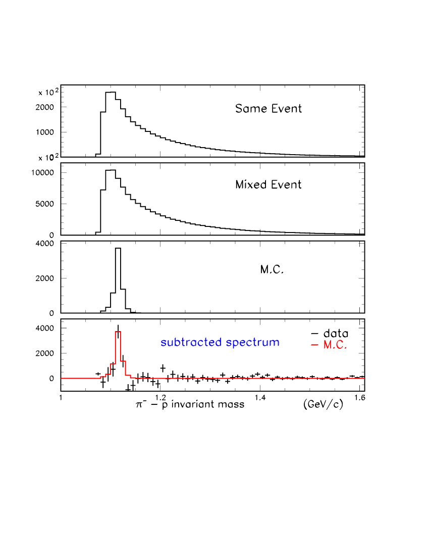
FIG. 2.: The top panel shows the invariant mass spectrum for p - $\pi^{-}$ coming from the same event. The second panel shows the invariant mass spectrum for p - $\pi^{-}$ coming from different events. The following panel shows the M.C. $\Lambda$ signal. The bottom panel has the subtracted invariant mass spectrum for p - $\pi^{-}$. The solid histogram overlaid on the data is the M.C. $\Lambda$ signal

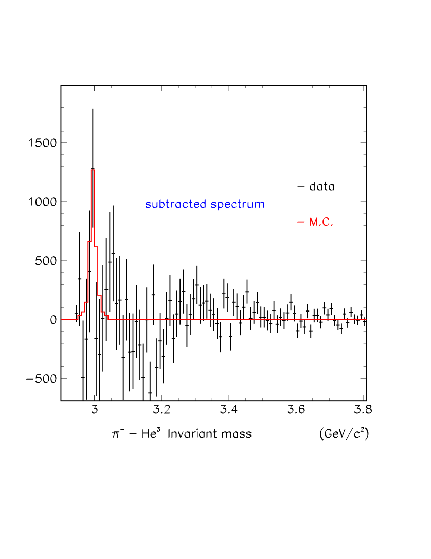
FIG. 3.: Subtracted invariant mass spectrum for ${}^{3}He$ - $\pi^{-}$ when strict hodoscope cuts are applied on the data. The solid histogram overlaid on the data is the M.C. ${}^{3}_{\Lambda}H$ signal normalized so that the peak bin matches the data.

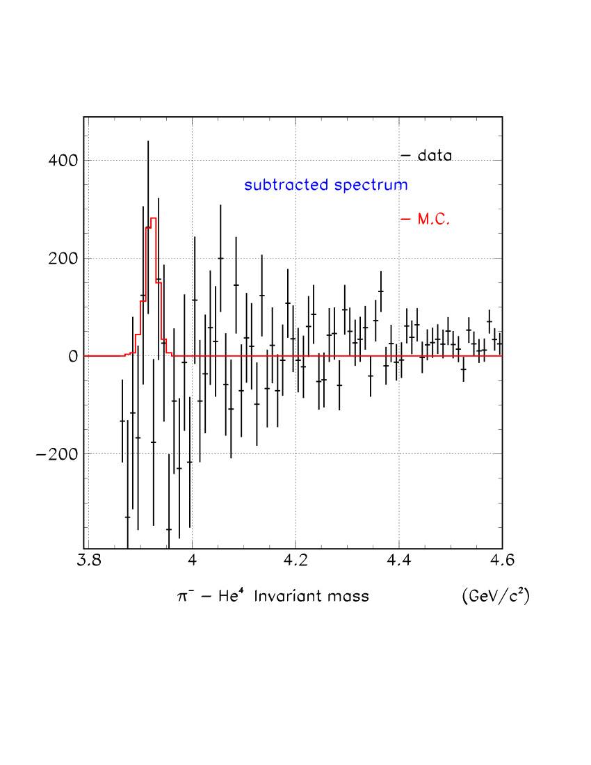
FIG. 4.: Subtracted invariant mass spectrum for ${}^{4}He$ - $\pi^{-}$ when strict hodoscope cuts are applied on the data. The solid histogram overlaid on the data is the M.C. ${}^{4}_{\Lambda}H$ signal

rapidity	1.6 - 2.6
$p_{T}$ (GeV/c)	0 - 1.5
$N_{event}$	$13.5\times 10^{9}$
$N_{count}$	$1220\pm 854$
$\epsilon_{total}=\epsilon_{acc}\times\epsilon_{LET}\times\epsilon_{ADDMC}\times\epsilon_{method}$	$1.96\times 10^{-4}$
detector efficiency: $\eta_{det}$	$0.82^{2}$
charge cut efficiency: $\eta_{q}$	0.84
target absorption probability: $\eta_{targ}$	0.78
$\chi^{2}$ cut efficiency: $\eta_{\chi^{2}}$	0.90
invariant yield $(GeV/c)^{-2}$	$(5.27\pm 4.04)\times 10^{-4}$

TABLE I.: Efficiencies and invariant yields for ${}^{3}_{\Lambda}H$ in $10\%$ most central Au-Pt collisions in units of $c^{2}/GeV^{2}$ for y:1.6-2.6 and $p_{T}$: 0-1.5 GeV/c

rapidity	1.8 - 2.6
$p_{T}$ (GeV/c)	0 - 1.5
$N_{event}$	$13.5\times 10^{9}$
$\epsilon_{total}=\epsilon_{acc}\times\epsilon_{LET}\times\epsilon_{ADDMC}\times\epsilon_{method}$	$9.3\times 10^{-4}$
detector efficiency: $\eta_{det}$	$0.82^{2}$
charge cut efficiency: $\eta_{q}$	0.84
target absorption probability: $\eta_{targ}$	0.89
$\chi^{2}$ cut efficiency: $\eta_{\chi^{2}}$	0.90

TABLE II.: Efficiencies for the ${}^{4}_{\Lambda}H$ in $10\%$ most central Au-Pt collisions in units of $c^{2}/GeV^{2}$ for y:1.8-2.6 and $p_{T}$: 0-1.5 GeV/c

REFERENCES

- [1] Present address: Vanderbilt University, Nashville, Tennessee 37235
- [2] Present Address: Istituto di Cosmo-Geofisica del CNR, Torino, Italy / INFN Torino, Italy
- [3] Present Address: Anderson Consulting, Hartford, CT
- [4] Present address: Univ. of Denver, Denver CO 80208
- [5] Deceased.
- [6] Present address: Argonne National Laboratory, 9700 S. Cass Ave., Argonne, Illinois 60439
- [7] Present address: Cambridge Systematics, Cambridge, MA 02139
- [8] Present address: McKinsey & Co., New York, NY 10022
- [9] Present address: Department of Radiation Oncology, Medical College of Virginia, Richmond VA 23298
- [10] Present address: University of Tennessee, Knoxville TN 37996
- [11] Present address: Geology and Physics Dept., Lock Haven University Lock Haven, PA 17745
- [12] Present address: Institut de Physique Nucléaire, 91406 Orsay Cedex, France
- [13] Present Address: Institute for Defense Analysis, Alexandria VA 22311
- [14] Present Address: MIT Lincoln Laboratory, Lexington MA 02420-9185
- [15] Present address: Brookhaven National Laboratory, Upton, New York 11973
- [16] J. Schaffner, H. Stocker (Frankfurt U.), C. Greiner, Phys. Rev. C 46(1992) 322.
- [17] E. Witten, Phys. Rev. D 30(1984) 272.
- [18] E. Farhi and R. L. Jaffe, Phys. Rev. D 30(1984) 2379.
- [19] R. L. Jaffe, Phys. Rev. Let. 38(1977) 195.
- [20] T. A. Armstrong et al., Phys. Rev. Lett. 79(1997) 3612.
- [21] T. A. Armstrong et al., Nucl. Phys. A625(1997) 494.
- [22] T. A. Armstrong et al., Phys. Rev. C 63(2001) 054903.
- [23] H. Liu and G. Shaw, Phys. Rev. D 30(1984) 1137.
- [24] H.J. Crawford, Mukesh S. Desai, Gordon L. Shaw, Phys. Rev. D 45(1992) 857.
- [25] C. Greiner and J. Schaffner, e-print archive: nucl-th/9801062.
- [26] A.J. Baltz, C.B. Dover, S.H. Kahana, Y. Pang, T.J. Schlagel, E. Schnedermann, Phys. Lett. B 325(1994) 7.
- [27] P. Braun-Munzinger, J. Stachel, J.P. Wessels, N. Xu, Phys. Lett. B 344(1995) 43.
- [28] P. Braun-Munzinger, J. Stachel, J. Phys. G 21(1995) L17.
- [29] R. Rafelski and B. Muller, Phys. Rev. Lett. 48(1982) 1066.
- [30] R. Rafelski and B. Muller, Phys. Rev. Lett. 56(1986) 2334E.
- [31] T. A. Armstrong et al., Phys. Rev. C 61(2000) 064908.
- [32] T. A. Armstrong et al., Nucl. Inst. Meth. A437(1999) 222.
- [33] T. A. Armstrong et al., Nucl. Inst. Meth. A406(1998) 227.
- [34] T. A. Armstrong et al., Nucl. Inst. Meth. A421(1999) 431.
- [35] H. Kamada, J. Golak, K. Miyagawa, H. Witala, W. Glockle, Phys. Rev. C 57(1998) 1595.
- [36] W. Glckle, K. Miyagawa, H. Kamada, J. Golak, H. Witala, Nucl. Phys. A639(1998) 297c.
- [37] S. Ahmad, B.E. Bonner, S.V. Efremov, G.S. Mutchler, E.D. Platner, H.W. Themann, Nucl. Phys. A636(1998) 507.
- [38] J. Barrette et al., Phys. Rev. C 63(2001) 014902.
- [39] I. Kumagai-Fuse, S. Okabe, Y. Akaishi, Nucl. Phys. A585(1995) 365c.
- [40] H. Outa, M. Aoki, R.S. Hayano, T. Ishikawa, M. Iwasaki, A. Sakaguchi, E. Takada, H. Tamura, T. Yamazaki, Nucl. Phys. A639(1998) 251c.
- [41] Particle Data Group, Phys. Rev. D 45(1992) III.39.
- [42] R. Scheibl and U. Heinz, Phys. Rev. C 59(1999) 1585.
- [43] Hidekatsu Nemura, Yasuyuki Suzuki, Yoshikazu Fujiwara, Choki Nakamoto, Prog. Theor. Phys. 103(2000) 929.
- [44] J. Barrette et al., Phys. Rev. C 60(1999) 054905.
- [45] J. Barrette et al., Phys. Rev. Lett. 78(1997) 2916.
- [46] M. Lisa et al., Nucl. Phys. A661(1999) 444.
- [47] D. Miskowiec et al., Nucl. Phys. A610(1996), 227c.
- [48] K. Filimonov et al., Nucl. Phys. A661(1999) 198.
- [49] T. A. Armstrong et al., Phys. Rev. Lett. 83(1999) 5431.
- [50] T. A. Armstrong et al., to be published in Phys. Rev. C