Separation of the Longitudinal and Transverse Cross Sections
in the ${p(e,e^{\prime}K^{+})}\Lambda$ and ${p(e,e^{\prime}K^{+})}\Sigma^{0}$ Reactions

Abstract

We report measurements of cross sections for the reaction $p$($e$,$e^{\prime}K^{+}$)Y, for both the $\Lambda$ and $\Sigma^{0}$ hyperon states, at an invariant mass of $W$=1.84 GeV and four-momentum transfers $0.5<Q^{2}<2$ (GeV/c)². Data were taken for three values of virtual photon polarization $\epsilon$, allowing the decomposition of the cross sections into longitudinal and transverse components. The $\Lambda$ data is a revised analysis of prior work, whereas the $\Sigma^{0}$ results have not been previously reported.

I Introduction

Electromagnetic production of strange baryons has long been of interest because of the fact that such data can provide unique information about the flavor dependence of nucleon excited states, eventually leading to a better understanding of the theory of QCD. Unfortunately, progress in understanding the production mechanism has been slow, in no small part because of the lack of high quality data. With the recent availability of a high quality, continuous electron beam at Jefferson Laboratory, precise new measurements are now achievable over a wide kinematic range gnprl ; JLABK . In addition to providing information on the elementary production reaction, such data will also be a benchmark for future investigations of hyperon-nucleon interactions with nuclear targets.

In this paper, we present new cross section data on the reaction $p(e,e^{\prime}K^{+})\Sigma^{0}$ from Jefferson Lab experiment E93-018, that were acquired at values of the square of four-momentum transfer, $Q^{2}$, between 0.5 and 2.0 (GeV/c)². At each value of $Q^{2}$, cross sections were obtained at three different values of the virtual photon polarization $\epsilon$, allowing a separation of the cross section into its longitudinal (L) and transverse (T) components. Results for the $\Lambda$ channel were previously reported in Ref. gnprl . However, in order to provide an internally consistent comparison between the two reaction channels, we also present a reanalysis of the $\Lambda$ data. The differences between the two analyses will be discussed in detail in section IV: here we use a direct comparison of the experimental data to simulated yields in order to extract the cross section. The result is a significantly smaller longitudinal contribution and a weaker $Q^{2}$ dependence than was previously reported. After a brief introduction and a detailed description of the experiment and analysis, the data will be compared to isobaric models of meson electroproduction described below.

Exploratory measurements of kaon electroproduction were first carried out between 1972 and 1979 bebek-lt ; brauel . In Ref. bebek-lt the longitudinal and transverse contributions to the $\Lambda$ and $\Sigma^{0}$ cross sections were separated for three values of $Q^{2}$. Two values of $\epsilon$ were measured for each kinematic setting with relatively poor statistical precision, and the uncertainties in the L/T separated results were large. In Ref. brauel , the measurements were focused on pion electroproduction, but a sample of kaons was also acquired, from which cross sections were extracted. These measurements provided the first determination of the qualitative behavior of the kaon cross sections and were the basis for the development of modern models of kaon electroproduction.

Theoretical models all attempt to reproduce the available data from both kaon production and radiative kaon capture, while maintaining consistency with SU(3) symmetry constraints on the coupling constants wjc1992 ; cwj1993 . The energy regime addressed by these models is low enough that they are formulated using meson-nucleon degrees of freedom. The most recent theoretical efforts can be divided into two categories, isobaric models and those that use Regge trajectories.

The approach taken in the isobaric models is to explicitly calculate kaon production amplitudes from tree-level (i.e., only one particle exchanged) processes. A typical selection of diagrams considered is depicted in Figure 1. For example, in David et al. saclay-lyon , the authors sum over $s$-channel nucleon resonances up to and including spin 5/2, $u$-channel hyperon resonances of spin 1/2, and $t$-channel kaon resonances K^∗(892) and K1(1270). In the WJC model wjc1992 , a different selection of $s$ and $u$ channel resonances is included (both limited to spin 3/2). Mart et al. Mar00 include the lowest lying $S$- and $P$-wave resonances, plus an additional resonance $D_{13}$ for which there appears to be evidence from kaon photoproduction Tra98 , although alternative interpretations of the data have been put forth in Sag01 and Jan02 .

The various isobaric models share the property that they initially include only spin 1/2 baryonic resonances (although the specific resonances differ) and determine the remaining coupling constants from performing phenomenological fits to the data. The coupling constants, which are the parameters of the theory, are not well-constrained due to the lack of available data. Because of this, one sees differences in the various models for quantities such as $g_{\scriptscriptstyle K\Lambda N}$. One issue that these differences reflect is that the various models disagree on the relative importance of the resonances entering the calculation. Further details on the various isobaric models can be found in wjc1992 ; saclay-lyon ; adelseck-saghai ; mbh .

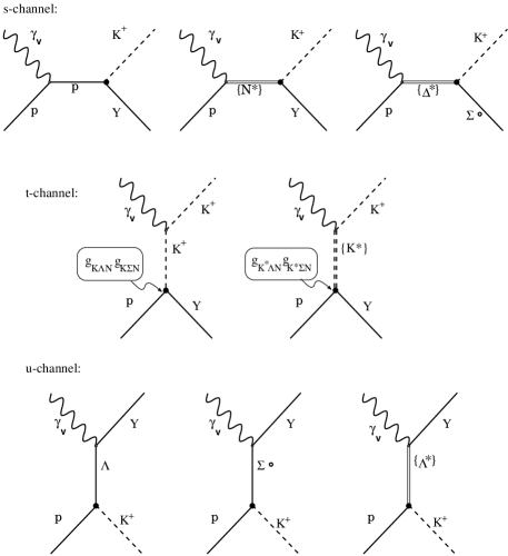
Figure 1: Examples of Feynman diagrams for kaon electroproduction considered in the isobaric models. The couplings in the $t$-channel ($g_{\scriptscriptstyle K\Lambda N}$, etc…) are shown explicitly. Note that the $s$-channel processes involving $\Delta^{*}$ resonances are forbidden by isospin conservation for $\Lambda$ production.

Models based on Regge trajectories reggetheory were developed in the early 1970’s to describe pion photoproduction data, of which there is a relative abundance. This approach has recently been revisited by Vanderhaegen, Guidal, and Laget (VGL) vgl-electroproduction . Here, the standard single particle Feynman propagator, $1/(t-m^{2})$, is replaced by a Regge propagator that accounts for the exchange of a family of particles with the same internal quantum numbers vgl1 . The extension of the photoproduction model to electroproduction is accomplished by multiplying the gauge invariant $t$-channel K and K^∗ diagrams by a form factor (the isobaric models such as WJC also include electromagnetic form factors, however the functional forms used differ between models wjc1992 ; adelseck-saghai ). For the VGL model this is given as a monopole form factor,

$$F_{\scriptscriptstyle K,K^{*}}(Q^{2})=\frac{1}{1+Q^{2}/\Lambda^{2}_{\scriptscriptstyle K,K^{*}}}\,\,,$$ (1)

where $\Lambda^{2}_{\scriptscriptstyle K,K^{*}}$ are mass scales that are essentially free parameters, but can be fixed to fit the high $Q^{2}$ behavior of the separated electroproduction cross sections, $\sigma_{\scriptscriptstyle{T}}$ and $\sigma_{\scriptscriptstyle{L}}$. For both the isobaric and Regge approaches, precise experimental results for longitudinal/transverse separated cross sections are important for placing constraints on the free parameters within the models, hopefully giving insight into the reaction mechanisms.

An additional motivation for performing measurements of L/T separated cross sections in kaon electroproduction is to determine the $Q^{2}$ dependence of the K⁺ electromagnetic form factor. If it can be demonstrated that $\sigma_{L}$ is dominated by photon absorption on a ground state kaon, the K⁺ form factor can be extracted through a measurement of the $t$-dependence of the longitudinal component of the cross section. This technique has been used to determine the $\pi^{+}$ electromagnetic form factor, including a recent new measurement Vol01 . While the kaon form factor may not be able to be extracted from the data presented here, it is the subject of other recently completed measurements at Jefferson Laboratory Mar01 .

Finally, historically there has been interest in the ratio of $\Sigma^{0}/\Lambda$ transverse cross sections, which is linked to contribution of sea quarks to nucleon structure Cley75 ; Nach74 . Within the context of the parton model, isospin arguments would lead one to expect the $\Sigma^{0}/\Lambda$ transverse cross section ratio at forward kaon CM angles to approach 0 with increasing Bjorken $x$ if the kaon production mechanism is dominated by the photon interacting with single valence $u$ quark. When sea quarks are included in the nucleon’s initial state, the approach to 0 is expected to be more rapid. Measurement of of $\sigma_{\scriptscriptstyle{T}}(\Sigma^{0})/\sigma_{\scriptscriptstyle{T}}(\Lambda)$ over a broad range of $x$ may provide information about the intrinsic $\overline{s}$$s$ content of the proton.

I.1 Elementary Kaon Electroproduction

The elementary kaon electroproduction reaction studied here,

$e$ + $p$ $\rightarrow$ $e^{\prime}$ + $K^{+}$ + ($\Lambda$ or $\Sigma^{0}$) ,

is shown in Figure 2. An incident electron ($e$) with lab energy $E$, scatters by radiating a virtual photon ($\gamma_{v}$). The scattered electron ($e^{\prime}$) travels at a polar angle $\theta_{e}$ in the Laboratory frame with respect to the direction of the incident beam, defining the scattering plane. The virtual photon carries momentum $\vec{q}$ and energy $\nu$ and interacts with a target proton to form a kaon (K⁺) and a hyperon (Y, here either a $\Lambda$ or $\Sigma^{0}$). The kaon travels at a polar angle $\theta_{\scriptscriptstyle{qK}}$ in the Laboratory frame with respect to the virtual photon direction and is also detected. The reaction plane, defined by the produced kaon and produced hyperon, makes an angle $\phi$ with respect to the scattering plane.

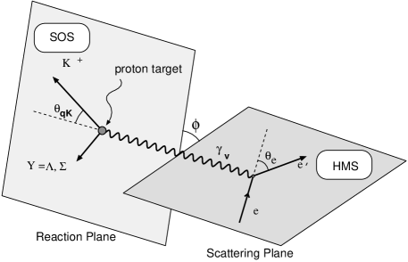
Figure 2: Definition of the kaon electroproduction reaction. Note the azimuthal angle, $\phi$, between the scattering and reaction planes with respect to the direction of the virtual photon.

The exclusive five-fold differential electroproduction cross section can be expressed in terms of a virtual photoproduction cross section, $\frac{d^{\,2}\sigma}{d\Omega_{\scriptscriptstyle K}^{*}}$, multiplied by a virtual photon flux factor, $\Gamma_{0}$ devlyth . The cross section is written in terms of the scattered electron energy, $E^{\prime}$, electron Lab frame solid angle, $d\Omega^{\prime}_{e}\equiv d\cos\theta_{e}\,d\phi_{e}\,$, and kaon Center-of-Momentum frame (CM) solid angle, $d\Omega_{\scriptscriptstyle K}^{*}\equiv d\cos\theta_{\scriptscriptstyle qK}^{*}\,d\phi\,$ as

$$\frac{d^{\,5}\sigma}{dE^{\prime}d\Omega^{\prime}_{e}d\Omega_{\scriptscriptstyle K}^{*}}=\Gamma_{0}(E^{\prime},\Omega^{\prime}_{e})\,\left(\frac{d^{\,2}\sigma}{d\Omega_{\scriptscriptstyle K}^{*}}\right)\,\,,$$ (2)

with

$$\Gamma_{0}(E^{\prime},\Omega^{\prime}_{e})=\frac{\alpha}{2\pi^{2}}\,\frac{(W^{2}-m_{p}^{2})}{2\,m_{p}}\,\frac{E^{\prime}}{E}\,\frac{1}{Q^{2}}\,\frac{1}{(1-\epsilon)}\,.$$ (3)

Here the CM frame is that of the (virtual photon + proton) system, and that the CM frame counterparts to Lab variables will be denoted with an asterisk superscript. In this expression, $\alpha$ is the fine structure constant ($\approx$1/137), $m_{p}$ is the proton mass, $W$ is the total energy of the (virtual photon + proton) system, $Q^{2}$ is the square of the four-momentum transfer carried by the virtual photon, and $\epsilon$ is the polarization of the virtual photon, given by

$$\epsilon=\frac{1}{1+2\,\frac{|\mathbf{q}|^{2}}{Q^{2}}\,\tan^{2}\frac{\theta_{e}}{2}}\,\,,$$ (4)

where $\mathbf{q}$ is the virtual photon three-momentum.

Because the beam and target were unpolarized, and no outgoing polarization was measured, the virtual photoproduction cross section can be decomposed into four terms:

$$\frac{d^{\,2}\sigma}{d\Omega_{\scriptscriptstyle K}^{*}}=\sigma_{\scriptscriptstyle T}+\epsilon\>\sigma_{\scriptscriptstyle L}+\sqrt{2\epsilon(\epsilon+1)}\>\sigma_{\scriptscriptstyle LT}\cos\phi+\epsilon\>\sigma_{\scriptscriptstyle TT}\cos 2\phi\,\,,$$ (5)

where $\sigma_{\scriptscriptstyle T}$ is the cross section due to transversely polarized virtual photons, $\sigma_{\scriptscriptstyle L}$ is due to longitudinally polarized virtual photons, and $\sigma_{\scriptscriptstyle LT}$ and $\sigma_{\scriptscriptstyle TT}$ are interference terms between two different polarization states. If one integrates the cross section over all $\phi\in(0,2\pi)$, the interference terms vanish leaving only the combined contributions from the transverse and longitudinal cross sections, $\sigma_{\scriptscriptstyle T}+\epsilon\sigma_{\scriptscriptstyle L}$. By measuring the cross section at several values of the virtual photon polarization, $\epsilon$, the cross sections $\sigma_{\scriptscriptstyle T}$ and $\sigma_{\scriptscriptstyle L}$ can be separated. The experimental setup described here was such that at each of the four values of $Q^{2}$, the full range in $\phi\in(0,2\pi)$ was accessible at three different values of the virtual photon polarization, $\epsilon$, as listed in Table 1. The data were fitted using the linear dependence between ($\sigma_{\scriptscriptstyle T}+\epsilon\sigma_{\scriptscriptstyle L}$) and $\epsilon$. The intercept and slope of the fitted line were used to extract $\sigma_{\scriptscriptstyle T}$ and $\sigma_{\scriptscriptstyle L}$ for each $Q^{2}$, for both the $\Lambda$ and $\Sigma^{0}$ channels.

No.	$\langle Q^{2}\rangle$	$\langle W\rangle$	$\langle\epsilon\rangle$	$E$	PHMS	$\theta_{\scriptscriptstyle{\mathrm{HMS}}}$	PSOS	$\theta_{\scriptscriptstyle{\mathrm{SOS}}}$
	(GeV/c)2	GeV	(for $\Lambda$)	GeV	GeV/c		GeV/c
1	0.52	1.84	0.552	2.445	0.833	29.27∘	1.126	13.40∘
2	0.52	1.84	0.771	3.245	1.633	18.03∘	1.126	16.62∘
3	0.52	1.84	0.865	4.045	2.433	13.20∘	1.126	18.34∘
4	0.75	1.84	0.462	2.445	0.725	37.95∘	1.188	13.42∘
5	0.75	1.84	0.724	3.245	1.526	22.44∘	1.188	17.62∘
6	0.75	1.84	0.834	4.045	2.326	16.23∘	1.188	19.75∘
7	1.00	1.81	0.380	2.445	0.635	47.30∘	1.216	13.40∘
8	1.00	1.81	0.678	3.245	1.435	26.80∘	1.216	18.20∘
9	1.00	1.81	0.810	4.045	2.236	19.14∘	1.216	20.78∘
10	2.00	1.84	0.363	3.245	0.844	50.59∘	1.634	13.42∘
11	2.00	1.84	0.476	3.545	1.145	41.11∘	1.634	15.67∘
12	2.00	1.84	0.613	4.045	1.645	31.83∘	1.634	18.14∘

Table 1: Kinematical settings measured in E93-018. Note that there are three settings of the virtual photon polarization, $\epsilon$, for each of four values of $Q^{2}$. Data were taken in the $\Lambda$ and $\Sigma^{0}$ channels simultaneously. For ease of discussion, the settings have been labeled as Point 1 through Point 12 in increasing order of $Q^{2}$, and with increasing order of $\epsilon$ within each $Q^{2}$ setting. The quantities (P_HMS,$\theta_{\scriptscriptstyle{\mathrm{HMS}}}$) and (P_SOS,$\theta_{\scriptscriptstyle{\mathrm{SOS}}}$) are the central momentum and angle settings of the two spectrometers used for electron and kaon detection, respectively.

II Experimental Apparatus

Data collection for experiment E93-018 took place in Hall C of Jefferson Lab in 1996. A schematic top view showing the relation between the spectrometers and the beamline/target chamber is depicted in Fig. 3. The Continuous Wave (CW, 100% duty factor) electron beam delivered to Hall C consisted of 1.67 ps micropulses spaced approximately 2 ns apart arising from the 499 MHz RF structure of the accelerator, with beam energies between 2.4 and 4 GeV. The primary target was a (4.36 $\pm$ 0.01) cm long liquid hydrogen cryotarget with 0.01 cm aluminum end windows. Background from the end windows, always less than a few percent, was measured (and subtracted) using an aluminum target with approximately ten times the thickness of the target windows. The integrated beam current (10-40 $\mu$A) was measured to an accuracy of 1.5% using a pair of microwave cavities calibrated with a DC current transformer. In order to reduce target density fluctuations arising from beam heating, the beam was rastered in a 2$\times$2 mm² square pattern at the entrance to the target.

Figure 3: Schematic top view of Hall C spectrometer setup showing the location of the HMS and SOS relative to the target and incident beam.

The scattered electrons were detected in the High Momentum Spectrometer (HMS), consisting of three superconducting quadrupole magnets in sequence followed by a superconducting dipole, followed by a detector package situated near the focal plane of the optical system. The electroproduced kaons were detected in the Short Orbit Spectrometer (SOS). The SOS is a non-superconducting magnetic spectrometer with one quadrupole (Q) magnet followed by two dipoles (D and $\overline{\mathrm{D}}$) which share a common yoke. It was designed with a short flight path in order to allow for detection of unstable, short-lived particles, such as kaons or pions, with good efficiency. Selected properties of the two spectrometers are listed in Table 2.

Both spectrometers were equipped with multiwire drift chambers for particle tracking and segmented scintillator hodoscope arrays for time-of-flight (TOF) measurement and trigger formation. Additionally, the HMS had a combination of a gas-filled threshold Čerenkov detector and a lead-glass calorimeter for $e$/$\pi^{-}$ separation, while the SOS had a diffusely-reflecting aerogel threshold Čerenkov detector ($n=1.034$) for the purposes of K⁺/$\pi^{+}$ separation. A lucite Čerenkov detector was also in the detector stack. It was not used in the trigger or in the present analysis, but was included when determining the energy loss of the kaons passing through the detector. Detection efficiencies in both spectrometers were dominated by the track reconstruction efficiency, with additonal small losses due to the coincidence circuit and the data acquisition dead time (see Table 3).

	HMS	SOS
Maximum central momentum	7.5 GeV/c	1.75 GeV/c
Momentum acceptance	$\pm$10 %	$\pm$20 %
Ang. Acceptance (in-plane)	$\pm$28 mrad	$\pm$57 mrad
Ang. Acceptance (out-of-plane)	$\pm$70 mrad	$\pm$37 mrad
Solid Angle (4.36 cm LH2 target)	6.8 msr	7.5 msr
Optical length	26.0 m	7.4 m

Table 2: Selected properties of the HMS and SOS.

Property	Typical	Random	Scale
	Correction	Error	Error
HMS Tracking efficiency	0.91 - 0.98	0.5 %	—
SOS Tracking efficiency	0.83 - 0.93	1.0 %	—
HMS Trigger efficiency	1.0	0.1 %	—
SOS Trigger efficiency	1.0	0.1 %	—
Coincidence efficiency	0.950 - 0.985	0.5 %	—
TOF $\beta$ cut efficiency	0.96 - 0.99	0.7 %	—
HMS Elec. Live Time	0.996 - 1.000	0.1 %	—
SOS Elec. Live Time	0.973 - 0.990	0.1 %	—
Computer Live Time	0.91 - 1.00	0.3 %	—
Cointime cut efficiency	1.0	0.1 %	—
HMS Čerenkov efficiency	0.998	0.2 %	—
Aerogel cut efficiency	0.974	—	0.3 %
HMS Acceptance	—	—	2.0 %
SOS Acceptance	—	—	2.0 %
Cut variation	—	0.7 - 3.1 %	—
Cross section model	0.9 - 1.1	0.5 %	2.0 %
Radiative Correction	—	1.0 %	1.0 %
Cut variation ($m_{\scriptscriptstyle Y}$)	—	0.5 %	—
Uncert. in $\theta_{e}$		0.3 - 1.3 %
Acceptance $\times$ Rad Corr	1.2 - 1.4
Kaon Absorption	0.94 - 0.97	0.5 %	0.5 %
Kaon Decay	2.5 - 4.0	1.0 %	3.0 %
Decay Prod. K+ Mimic	0.990 - 0.995	0.5 %	—
Target Length/Density	—	—	0.4 %
Target Density Fluct.	0.992	0.4 %	—
Target Purity	0.998	—	0.2 %
Charge Measurement	—	—	1.5 %
Total		2.5 - 4.0 %	5.0 %

Table 3: Systematic corrections and errors in the E93-018 analysis.

III Data Analysis

The raw data were processed and combined with additional experimental information such as the momentum and angle settings of the spectrometers, detector positions, and beam energy to yield particle trajectories, momenta, velocities, energy deposition, and to perform particle identification. Physics variables (such as $Q^{2}$, $W$, $\theta_{e}$, $\mathbf{p_{\scriptscriptstyle{K}}}$, $\theta_{\scriptscriptstyle{qK}}$…) were determined for each event at the interaction vertex, and then yields of electroproduced kaons as a function of a given subset of these variables were calculated.

III.1 Kaon Identification

In the SOS spectrometer, the velocities of the detected particles were calculated using the timing information from the scintillator hodoscopes. Once the velocities were determined, two additional software cuts were implemented to select kaons out of the proton and pion backgrounds: a direct cut on the velocity as measured from TOF information (called $\beta_{\mathrm{tof}}$), which eliminated the protons and the majority of the pions, and a cut on the number of photoelectrons detected in the aerogel Čerenkov detector which eliminated the remaining pions. The cut on $\beta_{\mathrm{tof}}$ was implemented as a cut on the quantity ($\beta_{\mathrm{tof}}$ $-$ $\beta_{\mathrm{\scriptscriptstyle{K}}}$), where $\beta_{\mathrm{\scriptscriptstyle{K}}}$ is the velocity of the detected hadron as determined from the measured momentum under the assumption that the incident particle was a kaon, defined as:

$$\beta_{\mathrm{\scriptscriptstyle{K}}}\equiv\frac{|{\mathbf{p}}|}{E}=\frac{|{\mathbf{p}}|}{\sqrt{|{\mathbf{p}}|^{2}+m_{\scriptscriptstyle{K}}^{2}}}.$$ (6)

The unshaded spectrum in Fig. 4 shows the quantity ($\beta_{\mathrm{tof}}$ $-$ $\beta_{\mathrm{\scriptscriptstyle{K}}}$). In the analysis, a cut was placed at $|$ ($\beta_{\mathrm{tof}}$ $-$ $\beta_{\mathrm{\scriptscriptstyle{K}}}$) $|$ $<$ 0.04.

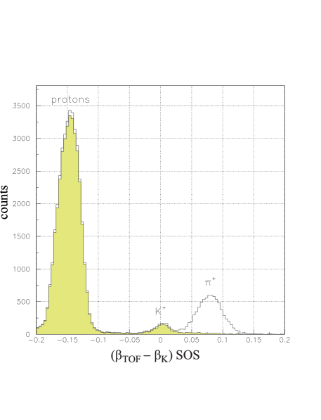
Figure 4: A typical $\beta_{\mathrm{tof}}-\beta_{\mathrm{\scriptscriptstyle{K}}}$ spectrum for the SOS, shown with (shaded) and without (unshaded) a software aerogel cut. The data in this figure and Figs. 5 and 6 are from kinematic point 2.

The second cut was on the number of photoelectrons detected in the aerogel Čerenkov. This eliminated most of the remaining background pions that the ($\beta_{\mathrm{tof}}$ $-$ $\beta_{\mathrm{\scriptscriptstyle{K}}}$) cut did not reject. The (very few) pions that survived both of these cuts were eliminated by the subtraction of the random background (see next section). The shaded region in Fig. 4 shows what remains after applying a cut requiring less than 3.5 photoelectrons in the aerogel detector.

III.2 Coincidence Cuts

The relative timing between the HMS and SOS signals was used to identify true kaon-electron coincidences. This coincidence time was corrected to account for variations in flight time arising from variations in particle velocity and path length through the spectrometers. An arbitrary offset was added such that events in which the electron and kaon originated from the same beam bunch would have a time of 0 ns. Figure 5 shows ($\beta_{\mathrm{tof}}$ $-$ $\beta_{\mathrm{\scriptscriptstyle{K}}}$) for the SOS plotted versus the corrected coincidence time for a single run, without having applied the previously described kaon identification cuts. Three horizontal bands of electron coincidences with protons, kaons, and pions are clearly identified, with the in-time pion and proton peaks offset from the in-time kaon peak by at least one beam bunch. Random coincidences, resulting from an electron and hadron from different beam bunches, have a coincidence time that is offset from the in-time peak by a multiple of $\sim$2 ns.

Figure 5: Plot of $(\beta_{\mathrm{tof}}-\beta_{\mathrm{\scriptscriptstyle{K}}})$ vs. SOS corrected coincidence time. Visible are three horizontal bands corresponding to protons, kaons, and pions. The coincidence time offset is chosen such that the in-time kaons appear at 0 ns. The correlation between coincidence time and $(\beta_{\mathrm{tof}}-\beta_{\mathrm{\scriptscriptstyle{K}}})$ in the proton bands reflects the range of proton velocities that could create a random coincidence with the electron arm within the trigger timing window.

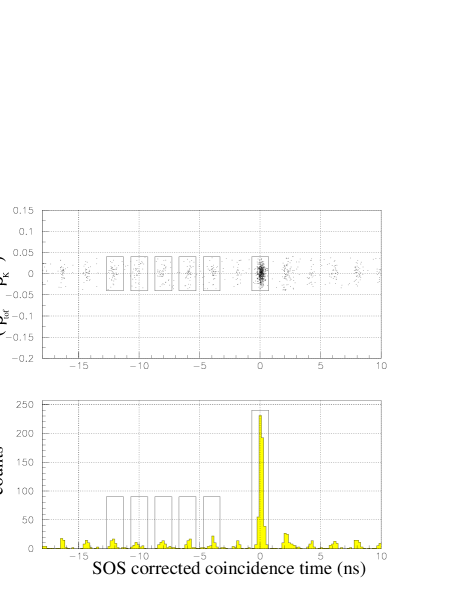
Figure 6: The upper panel shows $(\beta_{\mathrm{tof}}-\beta_{\mathrm{\scriptscriptstyle{K}}})$ vs. SOS corrected coincidence time, after applying cuts on $(\beta_{\mathrm{tof}}-\beta_{\mathrm{\scriptscriptstyle{K}}})$ and the aerogel. The single boxed region to the right is the in-time peak, and the five boxed regions to the left contain random coincidences. The lower panel shows the one-dimensional spectrum of SOS corrected coincidence times corresponding to the upper panel.

After applying the ($\beta_{\mathrm{tof}}$ $-$ $\beta_{\mathrm{\scriptscriptstyle{K}}}$) and aerogel cuts, the distribution shown in Fig. 5 reduces to that shown in Fig. 6(a). In Fig. 6(b) the one-dimensional projection of the upper half is shown. The in-time peak dominates over the purely random coincidences. The data were cut on the coincidence time around the peak, at $|\,\mathrm{cointime(SOS)}\,|<0.65\,\,\mathrm{ns}$. The random background was estimated by averaging over five bunches to the left of the in-time peak, and then subtracting it from the in-time yield to give the true kaon electroproduction yield.

III.3 Missing Mass Reconstruction

Once true $e$-$K$ coincidences were identified, the missing mass, $m_{\scriptscriptstyle{Y}}$, of the produced hyperon was reconstructed from measured quantities as

$$m_{\scriptscriptstyle Y}^{2}=-Q^{2}+m_{\scriptscriptstyle K}^{2}+2\,\nu\,m_{p}-2\,E_{\scriptscriptstyle K}(\nu+m_{p})-2\,\mathbf{q}\cdot\mathbf{p_{\scriptscriptstyle K}}\,\,,$$ (7)

where $(E_{\scriptscriptstyle K},\mathbf{p_{\scriptscriptstyle K}})$ is the kaon four-vector, and $(\nu,\mathbf{q})$ is the virtual photon four-vector.

Figure 7: An example of a missing mass spectrum for ${p(e,e^{\prime}K^{+})}$Y showing the $\Lambda$ and $\Sigma^{0}$ peaks and radiative tails. The vertical dashed lines are located at the accepted $\Lambda$ and $\Sigma^{0}$ masses. Note that this spectrum has already been corrected for random and target endcap yields.

Figure 7 is a histogram of the calculated missing mass, showing peaks at the $\Lambda$ and $\Sigma^{0}$ masses. The tail sloping off toward higher missing mass from each peak is due to the effects of radiative processes. A cut of $(1.100<m_{\scriptscriptstyle{Y}}<1.155)$ GeV was used to identify events with a $\Lambda$ in the final state, and $(1.180<m_{\scriptscriptstyle{Y}}<1.230)$ was used for the $\Sigma^{0}$ final state. The fraction of events lost due to the cut were accounted for in the data/Monte Carlo ratio used to determine the cross section. The $\Sigma^{0}$ analysis also required subtraction of the $\Lambda$ events in the radiative tail under the $\Sigma^{0}$ peak. After application of all cuts and identification of true ${p(e,e^{\prime}K^{+})}$Y events, the measured yields were corrected for losses due to detection efficiencies, kaon decay, and kaon absorption through the target and spectrometer materials. A summary of these corrections and their associated errors can be found in Table 3.

One of the largest corrections arose from the fact that kaons are unstable and have a short mean lifetime. As a result, a large fraction of the kaons created at the target decay into secondary particles before they can be detected. The survival fraction of the detected kaons is

$$\frac{N_{\mathrm{detected}}}{N_{\mathrm{at\,target}}}=\exp{{\left(-\frac{m_{\scriptscriptstyle K}\,d}{p_{\scriptscriptstyle K}\,\tau}\right)}}\,,$$ (8)

where $d$ is the distance traveled to the detector and $\tau\approx 12.4$ ns ($c\tau\approx 3.713$ m) is the mean lifetime of a kaon at rest PDB . The survival fraction varied between 0.25 and 0.4 for the range of kaon momenta detected here. Although the mean kaon decay correction is large, its uncertainty is small because both the kaon’s trajectory length and momentum were accurately determined event by event by the SOS tracking algorithm. An additional few percent correction was applied to account for the possibility that the decay products might actually be detected, mimicking an otherwise lost kaon event. This correction was estimated through the use of a Monte Carlo simulation of the six most likely decay processes as listed in PDB . Further details regarding the data analysis can be found in  rmmthesis .

IV Monte Carlo Simulation

In order to extract cross section information from the data, a detailed Monte Carlo simulation of the experiment was developed. The code was largely based on that developed in Ref. makinsthesis , which used the Plane Wave Impulse Approximation (PWIA) to model $A(e,e^{\prime}p)$ for various nuclei. The simulation included radiation, multiple scattering, and energy loss from passage through materials. It was updated with optical models of the HMS and SOS spectrometers and compared in detail with Hall C $(e,e^{\prime})$ and $(e,e^{\prime}p)$ data. For the present analysis it was additionally modified to simulate kaon electroproduction as well as kaon decay in flight. In the discussions that follow, the term “data” always refers to the measured experimental data yields, and the term “MC” always refers to the simulated events and yields.

IV.1 Event Generation

In the MC event generator, a random target interaction point is selected, consistent with the target length and raster amplitudes. The beam energy is then chosen about a central (input) value with a resolution $dE/E=\pm$0.05%. Events are randomly generated in the phase space including the spectrometer angles and electron momentum, from which the laboratory quantites $p_{e}$, $\theta_{e}$, $\phi_{e}$, $\theta_{\scriptscriptstyle K}$ and $\phi$ are computed. From the distribution of events, the phase space factor $\Delta V^{5}_{\mathrm{gen}}\equiv\Delta E^{\prime}\Delta\Omega^{\prime}_{e}\Delta\Omega_{\scriptscriptstyle K}$ is also computed. Each event is generated with unit cross section, with limits that extend well beyond the physical acceptances of the spectrometers even after the effects of energy loss, radiation and multiple scattering. From the scattered electron laboratory variables, the invariant quantities $Q^{2}$ and $W$ can be completely specified, as well as the kaon CM production angle $\theta_{\scriptscriptstyle qK}^{*}$, and the virtual photon polarization $\epsilon$.

For the kaon side, the hyperon $Y$ = $(\Lambda,\Sigma^{0})$ being generated is specified in the Monte Carlo input file. Because the kaon-hyperon production is a two-body reaction, the momentum of the outgoing kaon is fixed by knowledge of $W$. In the CM frame this relationship is

$$|{\mathbf{p^{*}_{\scriptscriptstyle K}}}|=\sqrt{\left(\frac{(W^{2}+m_{\scriptscriptstyle K}^{2}-m_{\scriptscriptstyle Y}^{2})}{2\,W}\right)^{2}-\,m_{\scriptscriptstyle K}^{2}}\,\,.$$ (9)

The remaining components of the kaon four-vector can be determined using the kaon CM angles $(\theta_{\scriptscriptstyle qK}^{*},\phi)$. In the Monte Carlo code, the laboratory kaon momentum is instead computed, from which CM quantities at the interaction vertex are calculated. The Jacobian that relates the kaon CM solid angle $\Delta\Omega_{\scriptscriptstyle K}^{*}$ to its laboratory counterpart is also specified since the reported cross sections are in the CM frame.

The radiative correction routines supplied in the original ($e$,$e^{\prime}p$) code of Ref. makinsthesis were based on the work of Mo and Tsai motsai , extended to be valid for a coincidence framework. Details of the corrections are documented in ent2002 . The procedure outlined in this reference was implemented for quasielastic proton knockout. In the present work, the same procedure was used with two modifications to consider kaon production: the mass of struck and outgoing particle was changed to $m_{K}$. This is appropriate for the pole contribution to the radiation, and better reproduces the data. In addition, the vertex reactions were modified to follow a parameterization of the ($e$,$e^{\prime}K$) cross section (discussed below).

Figure 8: Yield spectrum of missing mass comparing MC (solid line) to data (crosses) for $p$($e$,$e^{\prime}K^{+}$)$\Lambda$, on both linear (top panel) and logarithmic (bottom panel) scales, normalized by the extracted cross section. The data are from kinematic point 9.

Figure 8 shows the cross section weighted MC calculation of its yield, including the radiative tail (solid line), plotted on top of the measured data (crosses), on both linear and logarithmic scales. Although the resolution of the MC peak is slightly narrower than that of the data (a result of the spectrometer model), overall the agreement between the MC and data is quite good. The missing mass cut used to define the $\Lambda$ (1.100 $<m_{\scriptscriptstyle Y}<$ 1.155 GeV) was sufficiently wide that the extracted cross section was insensitive at the level of 0.5% to variations in the cut.

Figure 9 shows the sequential effect of placing the cuts on the experimental data from a single run. In the analysis, all of the cuts were systematically varied and their effects on the cross section noted. The standard deviation of the resulting cross sections was used as an estimate of the systematic error on the quoted cross section due to each cut. With the exception of a cut on $\theta_{\scriptscriptstyle{qK}}^{*}$, the cut values used were not kinematic dependent and are listed in table 4.

SOS momentum	$|\Delta P_{K}/P_{k}|<$ 17%
HMS momentum	$|\Delta P_{e}/P_{e}|<$ 8%
HMS out of plane angle	$|dx/dz|_{HMS}<$ 0.08 rad
HMS in-plane angle	$|dy/dz|_{HMS}<$ 0.04 rad
SOS out of plane angle	$|dx/dz|_{SOS}<$ 0.04 rad
SOS in-plane angle	$|dy/dz|_{SOS}<$ 0.07 rad
aerogel X (dispersion dir.)	-49.0 cm $<$ X $<$ 46.0 cm
aerogel Y	-14.0 cm $<$ Y $<$ 18.0 cm
Missing mass cut, $\Lambda$ only	1.100 GeV $<$ $m_{\scriptscriptstyle Y}$ $<$ 1.155 GeV
Missing mass cut, $\Sigma_{0}$ only	1.180 GeV $<$ $m_{\scriptscriptstyle Y}$ $<$ 1.230 GeV
$\theta_{\scriptscriptstyle{qK}}^{*}$ cut
kin 1/2/3	10/11/12∘
kin 4/5/6	10/12/14∘
kin 7/8/9	10/12/14∘
kin 10/11/12	12/14/16∘

Table 4: Fiducial cuts placed on both the data and Monte Carlo in determining the data/MC ratio. Additional cuts, as described in the text, were placed on data quantities, such as the number of aerogel and gas Čerenkov photoelectrons, coincidence time, and kaon velocity.

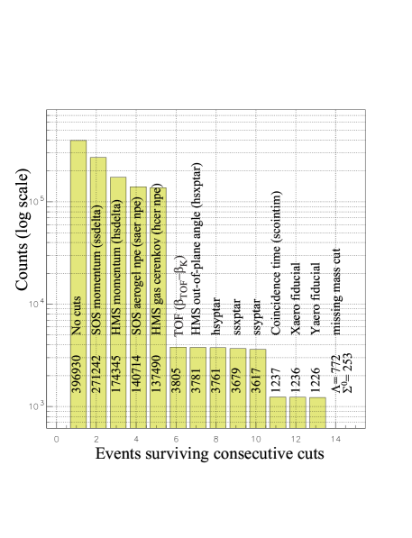
Figure 9: Histogram showing the cumulative effects of applying the cuts (note logarithmic scale). Shown are the number of counts surviving after applying the cuts as indicated from left to right, resulting in a final yield of 772 $\Lambda$ and 253 $\Sigma^{0}$. The data are from one run of kinematics 3.

IV.2 Equivalent Monte Carlo Yield

The equivalent experimental yield given by the MC can be expressed as

$$Y_{\mathrm{MC}}=L_{\scriptscriptstyle H} \times \int\left[\frac{d^{5}\sigma}{dE^{\prime}d\Omega^{\prime}_{e}d\Omega_{\scriptscriptstyle K}^{*}}\right]\left(\frac{d\Omega_{\scriptscriptstyle K}^{*}}{d\Omega_{\scriptscriptstyle K}}\right)$$ (10)

$$\times A(d^{\,5}V)\,R(d^{\,5}V)\,dE^{\prime}d\Omega^{\prime}_{e}d\Omega_{\scriptscriptstyle K}\,,$$

where $L_{\scriptscriptstyle H}$ is the experimental luminosity, $A$ is the acceptance function of the coincidence spectrometer setup, and $R$ is the radiative correction. The experimental luminosity is given by

$$L_{\scriptscriptstyle H}=C_{\mathrm{eff}}\,N_{\mathrm{beam}}\,N_{\mathrm{tgt}}\,,$$ (11)

where $C_{\mathrm{eff}}$ is a multiplicative factor containing all the global experimental efficiencies (such as the tracking efficiency, dead times, etc.), and $N_{\mathrm{beam}}$ and $N_{\mathrm{tgt}}$ are the number of incident electrons and the number of target nucleons/cm², respectively.

Substituting the virtual photoproduction cross section (Eq. 2) for the full electroproduction relation results in

$$Y_{\mathrm{MC}}=L_{\scriptscriptstyle H} \times \int\biggl{[}\Gamma_{0}(E^{\prime},\Omega^{\prime}_{e})\,\left(\frac{d^{\,2}\sigma}{d\Omega_{\scriptscriptstyle K}^{*}}\right)\left(\frac{d\Omega_{\scriptscriptstyle K}^{*}}{d\Omega_{\scriptscriptstyle K}}\right)\biggr{]}$$ (12)

$$\times A(d^{\,5}V)\,R(d^{\,5}V)\,dE^{\prime}d\Omega^{\prime}_{e}d\Omega_{\scriptscriptstyle K}.$$

In order to eventually extract cross sections by comparison with data, the MC yield was weighted by a cross section model that combines a single global factor $\sigma_{0}$, representing the cross section at specified values of $Q^{2}$, $W$ (denoted ($Q_{0}^{2}$,$W_{0}$)) and $\theta_{\scriptscriptstyle{qK}}^{*}=0^{\circ}$, with a function representing the event-by-event variation of the cross section across the experimental acceptance. The $\theta_{\scriptscriptstyle{qK}}^{*}$ behavior was represented by a variation in $t$, with $\theta_{\scriptscriptstyle{qK}}^{*}=0^{\circ}$ corresponding to the minimum accessible value of $t$, denoted $t_{min}$. The cross section model was based on previous data. This procedure is equivalent to replacing the cross section in Eq. 12 with the factorized expression

$$\left(\frac{d^{\,2}\sigma}{d\Omega_{\scriptscriptstyle K}^{*}}\right)\equiv\sigma_{0}\times\frac{f_{Q}(Q^{2})f_{W}(W)f_{t}(t)}{f_{Q}(Q_{0}^{2})f_{W}(W_{0})f_{t}(t_{min})}\,$$ (13)

where the various functions will be described below. The data constrain the choice of cross section models to those with relatively little variation in $Q^{2}$, $W$, or $t$ across the acceptance. As a result, the extracted cross section is not very sensitive to detailed behavior of the model.

The integral in Eq. 12 is evaluated numerically via the Monte Carlo simulation, with each Monte Carlo event being appropriately weighted with the radiative corrections, virtual photon flux, and the ($Q^{2}$,$W$,$t$) dependent terms of the cross section model. The influence of the acceptance function, $A$, arises through the fraction of generated events that successfully traverse the spectrometers and are reconstructed.

The MC equivalent yield then reduces to

$$Y_{\mathrm{MC}} = L_{\scriptscriptstyle H}\times\sigma_{0}\times\Delta V^{5}_{\mathrm{gen}}$$ (14)

$$\times \left(\frac{(\text{Number of MC successes})_{\mathrm{weighted}}}{\text{Number of MC tries}}\right)\,,$$

and by adjustment of $\sigma_{0}$ such that the yields of MC and measured data are equal (i.e., $Y_{\mathrm{MC}}=Y_{\mathrm{DATA}}$), the cross section $\sigma_{0}$ at the specified kinematics is determined.

IV.3 Cross Section Model

The previously existing world data were used to account for the cross section behavior across the acceptance. In Bebek et al. bebek-lt , where cross sections at $\theta_{\scriptscriptstyle{qK}}^{*}$=0^∘ were presented, the behavior of the cross section was parameterized as:

$$\frac{d^{\,2}\sigma}{d\Omega_{\scriptscriptstyle K}^{*}}\sim f_{Q}(Q^{2})\times f_{W}(W)\,,$$ (15)

where

$$f_{Q}(Q^{2})=\frac{1}{(Q^{2}+X)^{2}}$$ (16)

with $X=2.67$ for the $\Lambda$ channel, and $X=0.79$ for the $\Sigma^{0}$, and

$$f_{W}(W)=\frac{|\mathbf{p^{*}_{\scriptscriptstyle K}}|}{W(W^{2}-m_{p}^{2})}.$$ (17)

In a recent analysis of another set of kaon electroproduction data DMKthesis , it was shown that data at values of $W$ near the production threshold for the $\Lambda$ cross section were not accurately reproduced by the $W$ dependence in Eq. 17. In that analysis, a function of the following form was proposed, motivated by the hypothesis that there are possible resonance contributions to the cross section at lower $W$:

$$f_{\rm res}(W)=C_{1}f_{W}(W)+C_{2}\frac{\,\,A^{2}\,B^{2}}{(W^{2}-A^{2})^{2}+A^{2}B^{2}}$$ (18)

with $A$=$1.72$ GeV, $B$=$0.10$ GeV, $C_{1}$=$4023.9$ GeV² nb/sr, and $C_{2}$=$180.0$ GeV² nb/sr. This modified function was used here for the $\Lambda$ channel. In the $\Sigma$ channel, no such modification was found to be necessary to fit the existing data, so the original Bebek parameterization was used.

The $\theta_{\scriptscriptstyle{qK}}^{*}$ behavior was estimated using the results of Brauel, et al. brauel :

$$2\pi\frac{d^{\,2}\sigma}{dtd\phi}\sim e^{-\xi|t|}\,,$$ (19)

where $\xi=2.1$ for the $\Lambda$, and $\xi=1.0$ for the $\Sigma^{0}$, with the Mandelstam variable $t$ defined as

$$t=-Q^{2}+m_{\scriptscriptstyle K}^{2}-2\,E_{\scriptscriptstyle K}^{*}\nu^{*}+2\,|\mathbf{q^{*}}||\mathbf{p_{\scriptscriptstyle K}^{*}}|\cos\theta_{\scriptscriptstyle{qK}}^{*}\,\,,$$ (20)

where $(E_{\scriptscriptstyle K}^{*},\mathbf{p_{\scriptscriptstyle K}^{*}})$ is the kaon four-vector in the CM frame, and $(\nu^{*},\mathbf{q^{*}})$ is the virtual photon four-vector in the CM frame. Using Eq. 20 one can relate the $t$ behavior to the $\theta_{\scriptscriptstyle{qK}}^{*}$ behavior as

$$f(\theta_{\scriptscriptstyle{qK}}^{*})=\frac{1}{2\pi}\,e^{-\xi|t|}\left(2|\mathbf{q^{*}}||\mathbf{p_{\scriptscriptstyle K}^{*}}|\right)\,\,.$$ (21)

At $\theta_{\scriptscriptstyle{qK}}^{*}=0^{{}^{\circ}}$, the variable $t$ becomes $t_{min}$ given by

$$t_{min}=-Q^{2}+m_{\scriptscriptstyle K}^{2}-2\,E_{\scriptscriptstyle K}^{*}\nu^{*}+2\,|\mathbf{q^{*}}||\mathbf{p_{\scriptscriptstyle K}^{*}}|\,\,,$$ (22)

resulting in a functional form of

$$\frac{f_{t}(t)}{f_{t}(t_{min})}=\frac{f(\theta_{\scriptscriptstyle{qK}}^{*})}{f(\theta_{\scriptscriptstyle{qK}}^{*}=0^{{}^{\circ}})}=e^{-\xi(|t|-|t_{min}|)}=f_{t}(t-t_{min})\,.$$ (23)

Note that $t_{min}$ is a function of $Q^{2}$ and $W$ through its dependence on $\nu^{*}$.

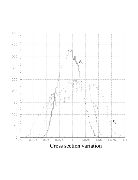
Figure 10: The cross section variation compared to its central value for the three values of $\epsilon$ at $Q^{2}=0.52$ (GeV/c)² (Points 1, 2, and 3).

In order to extract cross sections at the specific value of $\theta_{\scriptscriptstyle{qK}}^{*}=0^{{}^{\circ}}$, each event in the MC was weighted by the $Q^{2}$ and $W$ functions (defined in Eqs. 16 - 18), and by the $t$-dependent function in Eq. 23. Cross sections are thus presented not at fixed values of $t$ but instead at $t_{min}(Q^{2},W)$.

Figure 10 shows a histogram of the variation of the cross section weighting factor about its central value, on an event-by-event basis corresponding to the three values of $\epsilon$ at the $Q^{2}$ = 0.52 (GeV/c)² setting. The variation is largest at this lowest $Q^{2}$, and is essentially always less than $\pm$8%. The dependence of the extracted cross section on various deviations to this model was investigated in depth and the maximum observed effect was 2.3%.

IV.4 Differences from the Previous E93-018 Analysis

As discussed in the introduction, the cross sections for the $\Lambda$ channel that are presented here are significantly different than the earlier published data of Ref. gnprl . There are four main differences between the two analyses, three of which are somewhat trivial in nature. The first two have little influence on the unpolarized cross sections but are epsilon-dependent and therefore do affect the L/T separated data. Firstly, the radiative correction factors applied in Ref. gnprl were assumed to be constant for each kinematic setting at fixed $Q^{2}$, whereas they in fact vary by about 5% with $\epsilon$. Secondly, in Ref. gnprl it was assumed that the contributions from the interference structure functions $\sigma_{LT}$ and $\sigma_{TT}$ cancel within the acceptance and so no cut in $\theta^{*}_{qK}$ was applied. Since the acceptance is $\epsilon$ dependent, this assumption introduces an $\epsilon$-dependent bias. (With no $\theta_{\scriptscriptstyle{qK}}^{*}$ cut, the $\phi$ acceptance is not uniform, and the interference terms will give a net contribution to the cross section.) In the analysis presented here, such a cut was applied, and for each kinematic setting it was chosen as a compromise between optimizing the uniformity of the $\phi$ coverage and minimizing the effect of the cut on the extracted cross sections. Since the $\phi$-dependence of the acceptance arises naturally in the MC, the $\phi$-dependence of the acceptance was mostly removed in the data/MC ratio, and any residual dependence was attributed to the interference terms in the cross section.

Finally, in Ref. gnprl , a jacobian to convert kaon momentum to missing mass in the laboratory system was erroneously applied. The value of this jacobian varied with $Q^{2}$ from 1.95 to 2.8, but its influence was largely cancelled by the fourth difference which comes from how the phase-space acceptance for the detected kaons was handled. This last contribution could have a bearing on comparisons of the data reported here with calculations and with other kaon electroproduction experiments.

In principle, in a simulation of the $p(e,e^{\prime}K^{+})\Lambda$ reaction with the missing mass held fixed, and at fixed kaon production angle in the laboratory, there are two solutions to Eq. 9, corresponding to forward and backward going kaons in the CM frame. The analysis of Ref. gnprl made the fundamentally correct assumption that either of the two found solutions is possible. This is true in general, and is an appropriate assumption for a kaon electroproduction experiment in a large acceptance device. However, it is inconsistent with the generally biased preference to detect the “forward”-going kaon due to the limited momentum acceptance magnetic spectrometer. The procedure used in Ref. gnprl to account for both kaon momentum solutions led to an increase in the assumed phase space by a factor of two, and thus a reduction in the cross section of the same amount. This factor largely cancelled the effect from the jacobian.

One might argue that an experiment carried out with limited acceptance detectors does not truly measure an exclusive five-fold laboratory differential cross section, but rather a cross section solely related to the forward-going kaons in the center-of-mass frame. If one had perfect knowledge of the kaon electroproduction process, a simulated experiment taking the “backward”-going kaons into account could be carried out, from which one could obtain experimental laboratory cross sections that can be directly compared with theoretical calculations. Alternatively, additional experimental configurations could be chosen to measure the “backward”-going electroproduction cross sections. Obviously, large acceptance devices do not encounter this problem and have an advantage here. However, even in a complete experiment, it would be necessary to separate out the forward and backward going kaons, which correspond to different CM angles, when converting from the measured lab cross sections to the desired CM values.

In the present analysis, backward-going kaons were simulated and found to be well outside of the momentum acceptance of the kaon spectrometer, therefore taking only the forward-going solution was in fact the consistent way to match the true experimental conditions. It should also be noted that all previous electroproduction experiments with a magnetic spectrometer setup have reported exclusive five-fold differential electroproduction cross sections with the same biased preference.

V Results

The data and MC were binned in $\phi$ in order to study the effect of potential contributions from the interference terms to the extracted cross sections prior to carrying out the L/T separation. Cross sections were extracted by forcing the ratio of data to MC yields to be unity through adjustment of the overall normalization factor $\sigma_{0}$ in the MC bin-by-bin. After a first pass through the analysis, both the data and MC yields were stored in 8 bins of $\phi$. The ratio of data/MC was calculated in each bin yielding a zeroth order cross section for that bin. The procedure was then iterated, applying the extracted $(n-1)^{th}$ order cross section as a weighting factor for the yields in each $\phi$ bin using the generated values of the MC $\phi$ as the bin index. Typically the extracted cross section stabilized to within 0.1% of its value in three iterations. These final bin-by-bin values were fitted to a constant plus a harmonic $\phi$ dependent function of the form $A+B\cos\phi+C\cos 2\phi$ in order to extract $A=\sigma_{\scriptscriptstyle{T}}+\epsilon\sigma_{\scriptscriptstyle{L}}$. Note that with a single $\phi$ bin, the $\phi$ dependence should naturally cancel if the $\phi$ acceptance is uniform. This was true provided that the accepted events are restricted to forward values of $\theta_{\scriptscriptstyle qK}^{*}$. The extracted cross sections from a single bin in $\phi$ compared with 8 bins were unchanged at the level of 0.5% for the $\Lambda$ channel and at the level of 1.5% for the $\Sigma_{0}$ channel.

The choice of cut in $\theta_{\scriptscriptstyle qK}^{*}$ was kinematic dependent, and the values used are in Table 4. The $\phi$-dependent terms could not be quantitatively extracted due to the low statistics per bin and the poor $\phi$ reconstruction resolution for these small values of $\theta_{\scriptscriptstyle qK}^{*}$. However, the amplitude of $\cos\phi$ ($\cos 2\phi$) term was typically 10% (5%) of the unpolarized cross section.

The procedure for extracting the $\Sigma^{0}$ cross section was similar to that for the $\Lambda$, except that the $\Sigma^{0}$ yield was also corrected for the $\Lambda$ radiative tail beneath the $\Sigma^{0}$ peak in the missing mass spectrum. The $\Lambda$-specific MC was used to determine the number of background $\Lambda$ counts that were within $\Sigma^{0}$ cuts. The $\Lambda$-specific MC was weighted with the extracted $\Lambda$ cross section, binned in the same manner as the data, and was subtracted from each data bin. The upper half of Fig. 11 shows the combination of the $\Lambda$-specific and $\Sigma^{0}$-specific MC simulations plotted on top of the data missing mass. The lower half of the figure shows the remaining $\Sigma^{0}$ data after subtracting the $\Lambda$-specific MC, with the $\Sigma^{0}$-specific MC superimposed. Varying the $\Lambda$ cross section in the $\Sigma^{0}$ extraction analysis by $\pm$10% resulted in changes of less than 2% in the $\Sigma^{0}$ cross section. While the $\Lambda$ cross sections were typically determined to better than $\pm$10%, the contamination of the $\Lambda$ events in the $\Sigma^{0}$ yield comes from events which have undergone significant radiation and therefore the $\Lambda$ yield in that region is likely more sensitive to the details of the model in the Monte Carlo. An additional scale uncertainty proportional to the $\Lambda$ cross section uncertainty was thus applied to the $\Sigma^{0}$ results.

Figure 11: Use of the MC to correct for the $\Lambda$ radiative tail below the $\Sigma^{0}$ missing mass peak. The upper panel shows the combination of the $\Lambda$-specific and $\Sigma^{0}$-specific MC simulations (solid histogram) plotted on top of the data missing mass (crosses). The lower panel shows the remaining $\Sigma^{0}$ data after subtracting the $\Lambda$-specific MC, with the $\Sigma^{0}$-specific MC superimposed. The MC is normalized using the extracted $\Lambda$ and $\Sigma^{0}$ cross sections. The data are from kinematic point 3.

Typical values for all corrections to the data and/or the MC, along with the resulting systematic errors in the cross section, are shown in Table 3. The statistical errors for the various settings ranged from 1.0$-$3.1% for the $\Lambda$, and from 4.8$-$15% for the $\Sigma^{0}$. The systematic errors are broken down into “random” and “scale” errors. Since random errors affect each kinematic setting in an independent manner, they were retained for the linear fit of the L/T separation while the global errors that result in an overall multiplicative factor to the data were ignored for the fitting procedure, and applied as a scale uncertainty in the individual L/T cross sections. The sources of the errors in Table 3 are discussed in detail in rmmthesis .

V.1 $\Lambda$ and $\Sigma^{0}$ cross sections

The extracted p(e,e^′K⁺)$\Lambda$ and p(e,e^′K⁺)$\Sigma^{0}$ unseparated cross sections are given in Table 5. For the sake of comparison, the unseparated cross sections at the highest $\epsilon$ values (which were similar to those of the earlier data) are also shown in Figs. 12 and 13 along with the previous world data taken from bebek-prd0277 ; brownworlddata (also, see rmmthesis ). For the purposes of this plot, the E93-018 results have been scaled to $W$=2.15 GeV using the parameterization in bebek-lt (Equation 17) and include a 5% (6%) scale error for the $\Lambda$ ($\Sigma^{0}$) data. The previous world data shown in this plot have been scaled to $W$ = 2.15 GeV and $\theta_{\scriptscriptstyle{qK}}^{*}=0^{\circ}$ using equations 17 and 23. It should be emphasized that the data shown are at varying values of $t$, ranging from 0.05-3.0 GeV², so quantitative comparisons between data sets should be performed with care. The $Q^{2}$ dependent parameterization in Ref. bebek-prd0277 and shown here is for data at $\theta_{\scriptscriptstyle{qK}}^{*}=0^{\circ}$. Qualitatively good agreement is seen with previous data, and the new data do not significantly alter the $Q^{2}$ parameterization derived from older data sets.

	$\Lambda$ channel
$\langle Q^{2}\rangle$	$\langle W\rangle$	$-t_{min}$ (GeV)2	$\epsilon$	$\sigma_{\scriptscriptstyle{T}}+\epsilon\sigma_{\scriptscriptstyle{L}}$
GeV2	GeV			nb/sr
0.52	1.84	0.22	0.552	367.6 $\pm$ 12.0
			0.771	391.5 $\pm$ 12.3
			0.865	405.3 $\pm$ 13.1
0.75	1.84	0.30	0.462	329.7 $\pm$ 10.8
			0.724	357.4 $\pm$ 10.8
			0.834	381.1 $\pm$ 11.3
1.00	1.81	0.41	0.380	293.9 $\pm$ 10.4
			0.678	332.5 $\pm$ 11.3
			0.810	340.3 $\pm$ 11.8
2.00	1.84	0.74	0.363	184.5 $\pm$ 8.0
			0.476	200.6 $\pm$ 7.0
			0.613	202.9 $\pm$ 6.4
	$\Sigma^{0}$ channel
$\langle Q^{2}\rangle$	$\langle W\rangle$	$-t_{min}$ (GeV)2	$\epsilon$	$\sigma_{\scriptscriptstyle{T}}+\epsilon\sigma_{\scriptscriptstyle{L}}$
GeV2	GeV			nb/sr
0.52	1.84	0.31	0.545	75.4 $\pm$ 5.5
			0.757	87.3 $\pm$ 4.6
			0.851	86.2 $\pm$ 4.0
0.75	1.84	0.41	0.456	54.2 $\pm$ 4.0
			0.709	64.7 $\pm$ 3.3
			0.822	63.0 $\pm$ 2.7
1.00	1.81	0.55	0.375	37.9 $\pm$ 4.5
			0.663	43.6 $\pm$ 3.3
			0.792	42.4 $\pm$ 2.4
2.00	1.84	0.95	0.352	17.0 $\pm$ 2.8
			0.461	16.2 $\pm$ 2.5
			0.598	18.3 $\pm$ 1.6

Table 5: Results for the unseparated $p(e,e^{\prime}K^{+})\Lambda$ and $p(e,e^{\prime}K^{+})\Sigma^{0}$ cross sections used in the L/T separation: the uncertainties do not include the scale error of 5% for the $\Lambda$ channel and 6% for the $\Sigma^{0}$ channel. Cross sections were extracted at $\theta_{\scriptscriptstyle{qK}}^{*}=0^{\circ}$ and at the $W$ and $Q^{2}$ values in the table, using the procedure outlined in section IV.C. Note that because a single experimental setting was used to acquire both $\Lambda$ and $\Sigma^{0}$ data, the results are at different values of $-t_{min}$ for fixed $\theta_{\scriptscriptstyle{qK}}^{*}$.

Figure 12: Previous world data (open symbols: circles brownworlddata , squares bebek-74 , diamonds bebek-prd0277 ) with the addition of the highest-$\epsilon$ results of this analysis (solid points) scaled to $W$ = 2.15 GeV, $\theta_{\scriptscriptstyle{qK}}^{*}=0^{\circ}$, for the $p(e,e^{\prime}K^{+})\Lambda$ unseparated cross sections.

Figure 13: Previous world data (see caption for Fig. 12) with the addition of the highest-$\epsilon$ results of this analysis (solid points) scaled to $W$ = 2.15 GeV, $\theta_{\scriptscriptstyle{qK}}^{*}=0^{\circ}$, for the $p(e,e^{\prime}K^{+})\Sigma^{0}$ unseparated cross sections.

The unseparated cross sections are plotted as a function of $\epsilon$ in Figures 14 and 15. A linear least-squares fit was performed at each value of $Q^{2}$ to determine the best straight line ($\sigma~{}=~{}\sigma_{\scriptscriptstyle{T}}~{}+~{}\epsilon\sigma_{\scriptscriptstyle{L}}$) through the points. The resulting values of $\sigma_{\scriptscriptstyle{L}}$, $\sigma_{\scriptscriptstyle{T}}$, and $R$ = $\sigma_{\scriptscriptstyle{L}}/\sigma_{\scriptscriptstyle{T}}$ are shown in Table 6. Although only statistical and random systematic errors were used in the linear fit, the errors on the extracted values of $\sigma_{\scriptscriptstyle{L}}$ and $\sigma_{\scriptscriptstyle{T}}$ include the scale errors added in quadrature with the random errors. The quantity $R$ is insensitive to scale errors.

The separated cross sections $\sigma_{\scriptscriptstyle{L}}$ and $\sigma_{\scriptscriptstyle{T}}$ for the $\Lambda$ channel are plotted as a function of $Q^{2}$ in Figs. 16(a) and 16(b), respectively, along with other existing data. The equivalent plots for the $\Sigma^{0}$ channel are in Fig. 17. Photoproduction points from feller are also shown in the transverse components, taken at comparable values of $W$ and $\theta_{\scriptscriptstyle{qK}}^{*}\sim 30^{\circ}$. For these figures they are scaled to $W$ = 1.84 GeV, $\theta_{\scriptscriptstyle{qK}}^{*}=0^{\circ}$ (corresponding to an upward adjustment of 1.3 (1.1) for $\Lambda$ ($\Sigma^{0}$)). The third panel of each plot contains the ratio $R=\sigma_{\scriptscriptstyle{L}}/\sigma_{\scriptscriptstyle{T}}$ as a function of $Q^{2}$, along with data from bebek-lt . The curves shown are from the WJC model wjc1992 and from the unitary isobar model of Mart et al. with its default parameterizations Mar00 .

Finally, the ratio of $\Sigma^{0}$/$\Lambda$ separated cross sections $\sigma_{\scriptscriptstyle{L}}$ and $\sigma_{\scriptscriptstyle{T}}$ are shown plotted vs. $Q^{2}$ in Figs. 18(a) and 18(b), respectively, along with curves from the two models.

		$\Lambda$ channel
$\langle Q^{2}\rangle$	$\langle W\rangle$	$\sigma_{\scriptscriptstyle{L}}$ (nb/sr)	$\sigma_{\scriptscriptstyle{T}}$ (nb/sr)	R = $\sigma_{\scriptscriptstyle{L}}/\sigma_{\scriptscriptstyle{T}}$
0.52	1.84	118.3 $\pm$ 54.6	301.8 $\pm$ 40.1	0.39${}^{+0.27}_{-0.21}$
0.75	1.84	131.3 $\pm$ 40.5	267.5 $\pm$ 27.8	0.49${}^{+0.23}_{-0.18}$
1.00	1.81	112.4 $\pm$ 35.2	252.3 $\pm$ 22.1	0.45${}^{+0.19}_{-0.16}$
2.00	1.84	66.8 $\pm$ 40.4	163.8 $\pm$ 20.7	0.41${}^{+0.34}_{-0.26}$
		$\Sigma^{0}$ channel
$\langle Q^{2}\rangle$	$\langle W\rangle$	$\sigma_{\scriptscriptstyle{L}}$ (nb/sr)	$\sigma_{\scriptscriptstyle{T}}$ (nb/sr)	R = $\sigma_{\scriptscriptstyle{L}}/\sigma_{\scriptscriptstyle{T}}$
0.52	1.84	36.3 $\pm$ 22.2	56.9 $\pm$ 16.8	0.64${}^{+0.81}_{-0.45}$
0.75	1.84	24.0 $\pm$ 13.2	44.6 $\pm$ 9.5	0.54${}^{+0.52}_{-0.34}$
1.00	1.81	10.1 $\pm$ 12.1	35.1 $\pm$ 8.5	0.29${}^{+0.54}_{-0.33}$
2.00	1.84	7.5 $\pm$ 12.5	13.7 $\pm$ 6.6	0.55${}^{+2.15}_{-0.78}$

	Ratio of $\Sigma^{0}$ / $\Lambda$
$\langle Q^{2}\rangle$	$\langle W\rangle$	$\sigma_{\scriptscriptstyle{L}}(\Sigma^{0})/\sigma_{\scriptscriptstyle{L}}(\Lambda)$	$\sigma_{\scriptscriptstyle{T}}(\Sigma^{0})/\sigma_{\scriptscriptstyle{T}}(\Lambda)$
0.52	1.84	0.31 $\pm$ 0.24	0.19 $\pm$ 0.06
0.75	1.84	0.18 $\pm$ 0.11	0.17 $\pm$ 0.04
1.00	1.81	0.09 $\pm$ 0.11	0.14 $\pm$ 0.04
2.00	1.84	0.11 $\pm$ 0.20	0.084 $\pm$ 0.042

Table 6: L/T separated cross section results from this analysis for reactions p(e,e^′K⁺)$\Lambda$ and p(e,e^′K⁺)$\Sigma^{0}$, and for the ratio of $\Sigma^{0}$ to $\Lambda$ cross sections.

Figure 14: Cross sections as a function of $\epsilon$ for the $p(e,e^{\prime}K^{+})\Lambda$ process, shown with the linear fit to the data that allows separation into the longitudinal and transverse components.

Figure 15: Cross sections as a function of $\epsilon$ for the $p(e,e^{\prime}K^{+})\Sigma^{0}$ process. The lines are the fit to the data, allowing separation of the longitudinal and transverse components.

It should be noted that the data for E93-018 were taken in parallel with another experiment in which angular distributions of kaon electroproduction from hydrogen and deuterium were studied. In a few cases the kinematic settings were very similar, and comparisons were made with cross sections extracted from the analysis of DMKthesis ; jinseokthesis . They are in excellent agreement (within 2.5%), when scaled to the same $Q^{2}$ and $W$ values using Eq. 16 and 18.

Figure 16: Longitudinal (a) and transverse (b) cross sections for $p(e,e^{\prime}K^{+})\Lambda$ as a function of $Q^{2}$. The ratio is shown in panel (c). The data are compared to calculations of wjc1992 (solid line) and Mar00 (dashed line). The open diamond data are from bebek-lt , and the solid diamond photoproduction data point is from feller .

Figure 17: Longitudinal (a) and transverse (b) cross sections for $p(e,e^{\prime}K^{+})\Sigma^{0}$ as a function of $Q^{2}$. The ratio is shown in panel (c). The calculations are again from wjc1992 (solid line) and Mar00 (dashed line). The open diamond data are from bebek-lt , and the solid diamond photoproduction data point is from feller .

Figure 18: Ratio of $\Sigma^{0}$/$\Lambda$ cross sections as a function of $Q^{2}$, separated into longitudinal (a) and transverse (b) components, compared with the same two calculations as above.

V.2 Comparison with Calculations

As described in the introduction, several model calculations of $\Lambda$ and $\Sigma^{0}$ electroproduction cross sections, using parameters fit to previous data, are available. We have chosen to compare our data to the models in wjc1992 (WJC) and Mar00 , for which calculations were readily available in the form in which the data are presented here. The parameters of each model were constrained by global fits to previously obtained unpolarized photo- and electroproduction data, and, through crossing arguments, to kaon radiative capture.

For the $\Lambda$ channel, the WJC model reproduces reasonably well the trends in both the longitudinal and transverse components (Figs. 16(a) and 16(b), respectively), although the transverse component is underpredicted. The calculation of Ref. Mar00 qualitatively reproduces the transverse piece, which is constrained by the photoproduction point, but not the longitudinal component. One possible cause for the discrepancy could be the lack of knowledge of the $Q^{2}$ dependence of the baryon form factors entering in the $s$-channel cotanchprivcomm . In their study of kaon electroproduction, David et al., observed that $\sigma_{\scriptscriptstyle{L}}/\sigma_{\scriptscriptstyle{T}}$ was sensitively dependent on the choice of baryon form factors, while rather insensitive to the reaction mechanism saclay-lyon , whereas the unpolarized cross section alone did not depend strongly on the baryon form factors.

For ${p(e,e^{\prime}K^{+})}\Sigma^{0}$, the transverse component is underestimated by both models and thus the ratio is overestimated (see Fig. 17). The strong peak in $R$ implied by the WJC model is not observed in our data. The magnitude of this peak in the WJC model is very sensitive to the CM energy, $W$, of the reaction, indicating that there are strong resonance contributions in the model. As in the case of the $\Lambda$ channel, it is likely that the form factors and the strengths of the various resonances entering the model could be modified in order to give better agreement with the data. In general, models for the $\Sigma^{0}$ channel are harder to tune than for the $\Lambda$ because of the influence of isovector $\Delta$ resonances (of spin 1/2 and 3/2 in the model) in the $\Sigma^{0}$ channel and because of the lower quality/quantity of available data.

The ratio of the longitudinal cross sections for $\Sigma^{0}/\Lambda$ (Fig. 18(a)) appears to mildly decrease with increasing $Q^{2}$. This could arise, for example, from differences in the behavior of the $g_{\scriptscriptstyle\Sigma NK}(t)$ and $g_{\scriptscriptstyle\Lambda NK}(t)$ form factors, if the longitudinal response is dominated by $t$-channel processes.

We note that while Regge trajectory models are not expected to work well at the rather low CM energies of our data, which are still within the nucleon resonance region, our highest $Q^{2}$ results are in reasonable agreement with the calculation of vgl2 , both in the unseparated cross sections and in the L/T components. At lower momentum transfer our data indicate a larger longitudinal component to the $\Sigma^{0}$ cross sections than predicted by their model, perhaps indicative of the larger number of resonance contributions to the $\Sigma^{0}$ channel.

The ratio of the transverse cross sections for $\Sigma^{0}/\Lambda$ (Fig. 18(b)) shows a mild decrease above $Q^{2}\approx 0.52$ GeV². However, the inclusion of the DESY photoproduction data on the plot shows that there is likely a rapid decrease in $R_{T}$ for $Q^{2}$ below 0.5 (GeV/c)². This lower momentum region may be of interest for further study, particularly in the $\Sigma^{0}$ channel.

Conclusions

Rosenbluth separated kaon electroproduction data in two hyperon channels, $p\,(e,e^{\prime}K^{+})\Lambda$ and $p\,(e,e^{\prime}K^{+})\Sigma^{0}$, have been presented. These results are the most precise measurements of the separated cross sections $\sigma_{\scriptscriptstyle{T}}$ and $\sigma_{\scriptscriptstyle{L}}$ made to date, particularly for the $\Sigma^{0}$ channel, and will help constrain theoretical models of these electroproduction processes. Such data allow access to baryon excitations that couple strongly to final states with strangeness but weakly to $\pi$-N systems. They also allow the possibility of mapping out the $Q^{2}$ evolution away from the photoproduction point, thereby providing a means to extract electromagnetic form factors and detailed information about the excited state wave functions. Used in conjunction with models they will allow one to learn more about the reaction dynamics of strangeness production.

References

- (1) G. Niculescu et al., Phys. Rev. Lett. 81, 1805 (1998).
- (2) See, for example, Jefferson Laboratory experiments E89-004 (R. Schumacher), E89-043 (L. Dennis), E93-030 (K. Hicks), E99-006 and E00-112 (D. Carman), and E98-108 (P. Markowitz), and E91-016 (B. Zeidman, contact).
- (3) C. J. Bebek et al., Phys. Rev. D 15, 3082 (1977).
- (4) P. Brauel et al., Z. Phys. C3, 101 (1979).
- (5) R. A. Williams, C.-R. Ji, and S. R. Cotanch, Phys. Rev. C 46, 1617, (1992).
- (6) S. R. Cotanch, R. A. Williams, and C.-R. Ji, Physica Scripta 48, 217 (1993).
- (7) J. C. David, C. Fayard, G. H. Lamot, and B. Saghai, Phys. Rev. C 53 , 2613 (1996).
- (8) T. Mart and C. Bennhold, Phys. Rev. C 61, 012201(R) (2000). The code to calculate the cross sections at our specific kinematics was provided by T. Mart. At the time of this writing, the version of the code provided at http://www.kph.uni-mainz.de/MAID/kaon/kaonmaid.html had known errors and therefore was not used.
- (9) M. Q. Tran et al., SAPHIR collaboration, Phys. Lett. B445, 20 (1998).
- (10) B. Saghai, nucl-th/0105001.
- (11) S. Janssen, J. Ryckebusch, D. Debruyne, and T. Van Cauteren, Phys. Rev. C 66, 035202 (2002).
- (12) R. A. Adelseck and B. Saghai, Phys. Rev. C 42, 108 (1990).
- (13) T. Mart, C. Bennhold, and C. E. Hyde-Wright, Phys. Rev. C 51, R1074 (1995).
- (14) P. D. B. Collins, An Introduction to Regge Theory and High Energy Physics, (Cambridge University Press, Cambridge, 1977).
- (15) M. Vanderhaeghen, M. Guidal, and J.-M. Laget, Phys. Rev. C 57, 1454 (1998).
- (16) M. Guidal, J.-M. Laget, and M. Vanderhaeghen, Nucl. Phys. A627, 645 (1997).
- (17) J. Volmer et al., Phys. Rev. Lett. 86, 1713 (2001).
- (18) Jefferson Laboratory experiment E98-108 (P. Markowitz, contact).
- (19) J. Cleymans and F. Close, Nucl. Phys. B85, 429 (1975).
- (20) O. Nachtmann, Nucl. Phys. B74, 422 (1974).
- (21) R. C. E. Devenish and D. H. Lyth, Phys. Rev. D 5 47 (1972).
- (22) Particle Data Group, D.E. Groom et al., Eur. Phys. Jour. C15, 1 (2000).
- (23) R.M. Mohring, Ph.D. thesis, University of Maryland (1999), (unpublished). It should be noted that an error was recently found in the calculation of the kaon’s survival probability in the thesis analysis, which accounts for the majority of the difference between the cross sections presented here and those in the thesis.
- (24) N.C.R. Makins, Ph.D. thesis, Massachusetts Institute of Technology (1994), (unpublished). See also T. G. O’Neill, Ph.D. thesis, California Institute of Technology (1994), (unpublished).
- (25) Y. S. Tsai, Phys. Rev. 122, 1898 (1961), L. M. Mo and Y. S. Tsai, Rev. Mod. Phys. 41, 205 (1969).
- (26) R. Ent, B.W. Filippone, N.C.R. Makins, R.G. Milner, T.G. O’Neill, and D.A. Wasson, Phys. Rev. C 64 054610 (2001).
- (27) D. M. Koltenuk, Ph.D. thesis, University of Pennsylvania (1999), (unpublished).
- (28) C. J. Bebek et al., Phys. Rev. D 15, 594 (1977).
- (29) C. N. Brown et al., Phys. Rev. Lett. 28, 1086 (1972).
- (30) C. J. Bebek et al., Phys. Rev. Lett. 32, 21 (1974).
- (31) P. Feller et al., Nucl. Phys. B39, 413 (1972).
- (32) J. Cha, Ph.D. thesis, Hampton University (2001), (unpublished).
- (33) S. R. Cotanch, private communication (1999).
- (34) M. Guidal, J.-M. Laget, and M. Vanderhaeghen, Phys. Rev. C 61, 025204 (2000).