Quasi-free Compton Scattering and the Polarizabilities of the Neutron

Abstract

Differential cross-sections for quasi-free Compton scattering from the proton and neutron bound in the deuteron have been measured using the Glasgow/Mainz photon tagging spectrometer at the Mainz MAMI accelerator together with the Mainz 48 cm $\O$ $\times$ 64 cm NaI(Tl) photon detector and the Göttingen SENECA recoil detector. The data cover photon energies ranging from 200 MeV to 400 MeV at $\theta^{\rm LAB}_{\gamma}=136.2^{\circ}$. Liquid deuterium and hydrogen targets allowed direct comparison of free and quasi-free scattering from the proton. The neutron detection efficiency of the SENECA detector was measured via the reaction $p(\gamma,\pi^{+}n)$. The ”free” proton Compton scattering cross sections extracted from the bound proton data are in reasonable agreement with those for the free proton which gives confidence in the method to extract the differential cross section for free scattering from quasi-free data. Differential cross-sections on the free neutron have been extracted and the difference of the electromagnetic polarizabilities of the neutron has been determined to be $\alpha_{n}-\beta_{n}=9.8\pm 3.6\text{(stat)}\,{}^{+2.1}_{-1.1}\text{(syst)}\pm 2.2\text{(model)}$ in units of $10^{-4}\,\mathrm{fm^{3}}$. In combination with the polarizability sum $\alpha_{n}+\beta_{n}=15.2\pm 0.5$ deduced from photoabsorption data, the neutron electric and magnetic polarizabilities, $\alpha_{n}=12.5\pm 1.8\text{(stat)}\,{}^{+1.1}_{-0.6}\text{(syst)}\pm 1.1\text{(model)}$ and $\beta_{n}=2.7\mp 1.8\text{(stat)}\,{}^{+0.6}_{-1.1}\text{(syst)}\mp 1.1\text{(model)}$ are obtained. The backward spin polarizability of the neutron was determined to be $\gamma^{(n)}_{\pi}=(58.6\pm 4.0)\times 10^{-4}{\rm fm}^{4}$.

1 Introduction

The electromagnetic structure of the nucleon is a fascinating field of current research. At low energies, the electromagnetic structure may be parametrized by amplitudes for single-pion photoproduction arndt96 ; drechsel99 and by the invariant amplitudes for Compton scattering LPS97 . Instead of using these amplitudes in their general form, it has become customary to consider special properties of these amplitudes which have a transparent physical interpretation. These properties are given in terms of electromagnetic structure constants of which the E2/M1 ratio of the $p\to\Delta$ transition, the electric and magnetic polarizabilities $\alpha$ and $\beta$, respectively, and the spin polarizabilities $\gamma_{0}$ and $\gamma_{\pi}$, for the forward and backward direction, respectively, are the most prominent.

These electromagnetic structure constants have been studied for the proton for a long time, whereas the corresponding investigations for the neutron are only beginning. This contrasts with the fact that for their interpretation it is of great interest to know whether or not the proton and the neutron have the same or different electromagnetic structure constants. This is one reason to study the electromagnetic polarizabilities of the neutron in addition to those for the proton. Since Compton scattering experiments appeared too difficult, the first generation of investigations concentrated on the method of electromagnetic scattering of low-energy neutrons in the Coulomb field of heavy nuclei, investigated in narrow-beam neutron transmission experiments. The history of these studies is summarized in Refs. aleksandrov92 ; aleksandrov01 . The latest in a series of experiments have been carried out at Oak Ridge schmiedmayer91 and Munich koester95 leading to

$$\alpha_{n}=12.6\pm 1.5\pm 2.0$$ (1)

and

$$\alpha_{n}=0.6\pm 5,$$ (2)

respectively, in units of $10^{-4}\,\mathrm{fm^{3}}$ which will be used throughout in the following. The numbers given here have been corrected by adding the Schwinger term lvov93 $e^{2}\kappa^{2}_{n}/4M^{3}=0.6$, containing the neutron anomalous magnetic moment $\kappa_{n}$ and the neutron mass $M$. This term had been omitted in the original evaluation of these experiments. After including the Schwinger term the numbers are directly comparable with the ones defined through Compton scattering. This means that the difference between the electric polarizabilities obtained by the two methods, i.e. electromagnetic scattering of neutrons in a Coulomb field and Compton scattering, was only due to the incomplete formula used for the evaluation of the electric polarizabilities derived from electromagnetic scattering experiments, whereas the distinction between a Compton polarizability $\bar{\alpha}$ and a ”true” polarizability $\alpha_{0}$ was not justified. The main argument is that $\alpha_{0}$ is not an observable but merely a model quantity which requires great precautions when used in model calculations lee01a ; lee01b ; lee02 . This clarification makes it unnecessary to use different notations for the electric and magnetic polarizabilities depending on the definition. Therefore, we decided to use the simplest choice, i.e. $\alpha$ and $\beta$.

While the Munich result koester95 has a large error, the Oak Ridge result schmiedmayer91 is of very high precision. However, this high precision has been questioned by a number of researchers active in the field of neutron scattering enik97 . Their conclusion is that the Oak Ridge result schmiedmayer91 possibly might be quoted as $7\leq\alpha_{n}\leq 19$. Furthermore, it should be noted that electromagnetic scattering of neutrons in a Coulomb field does not constrain the magnetic polarizability $\beta_{n}$.

A pioneering experiment on Compton scattering by the neutron had been carried out by the Göttingen and Mainz groups using photons produced by the electron beam of MAMI A operated at 130 MeV rose90 . This experiment followed a proposal of Ref. levchuk94 to exploit the reaction $\gamma d\to\gamma np$ in the quasi-free kinematics, though there is an evident reason why such an experiment is difficult at energies below pion threshold. For the proton the largest portion of the polarizability-dependent cross section in this energy region stems from the interference term between the Born amplitude containing Thomson scattering as the largest contribution, and the non-Born amplitude containing the polarizabilities. For the neutron the Thomson amplitude vanishes so that the interference term is very small and correspondingly cannot be used for the determination of the neutron polarizabilities. This implies that the cross section is rather small being about 2–3 nb/sr at 100 MeV. The way chosen to overcome this problem was to use a high flux of bremsstrahlung without tagging rose90 ; levchuk94 . The result obtained in the experiment rose90 was

$$\alpha_{n}=10.7\,{}^{+3.3}_{-10.7}.$$ (3)

This means that the experiment was successful in providing a value for the electric polarizability and its upper limit but it did not determine a definite lower limit. The reason for this deficiency is that below pion threshold the neutron Compton cross section is practically independent of $\alpha_{n}$ if $0\lesssim\alpha_{n}\lesssim 10$ levchuk94 ; wissmann98 . In order to overcome this difficulty it was proposed to measure the neutron polarizabilities at energies above pion threshold with the energy range from 200 to 300 MeV being the most promising since there the cross sections are very sensitive to $\alpha_{n}$ levchuk94 ; wissmann98 . In principle, this method allows a separate extraction of $\alpha_{n}$ and $\beta_{n}$. However, it is more precise to use the Baldin sum rule prediction for the sum of the nucleon polarizabilities. A recent evaluation of this sum rule levc00 gives

$$\alpha_{p}+\beta_{p}=14.0\pm 0.3,$$ (4)

$$\alpha_{n}+\beta_{n}=15.2\pm 0.5.$$ (5)

A first experiment on quasi-free Compton scattering by the proton bound in the deuteron for energies above pion threshold was carried out at MAMI (Mainz) wissmann99 . This experiment served as a successful test of the method of quasi-free Compton scattering for determining $\alpha_{n}-\beta_{n}$. The result obtained form the quasi-free data, $\alpha_{p}-\beta_{p}=9.1\pm 1.7\text{(stat+syst)}\pm 1.2\text{(model)}$ proved to be in reasonable agreement with the world average of the free-proton data which is $\alpha_{p}-\beta_{p}=10.5\pm 0.9\text{(stat+syst)}\pm 0.7\text{(model)}$ according to the most recent analysis olmos01 . Later on this method was applied to the proton and the neutron bound in the deuteron at SAL (Saskatoon) kolb00 . In this experiment differential cross sections for quasi-free Compton scattering by the proton and by the neutron were obtained at a scattering angle of $\theta^{\text{LAB}}_{\gamma}=135^{\circ}$ for incident photon energies of 236 – 260 MeV, which were combined to give one data point of reasonable precision for each nucleon. From the ratio of these two differential cross sections a most probable value of

$$\alpha_{n}-\beta_{n}=12$$ (6)

was obtained with a lower limit of 0 and no definite upper limit. Combining their result kolb00 with that of Eq. (3) rose90 the authors obtained the following 1$\sigma$ constraints for the electromagnetic polarizabilities

$$7.6\leq\alpha_{n}\leq 14.0$$ (7)

and

$$1.2\leq\beta_{n}\leq 7.6.$$ (8)

It should be noted that coherent elastic (Compton) scattering by the deuteron provides a further method for determining the electromagnetic polarizabilities of the neutron. Measurements of differential cross sections of this process have been performed at Illinois lucas94 , SAL hornidge00 , and MAX-lab lundin02 . An evaluation of these experiments in the framework of the theoretical approach levc00 gives the following values for the neutron polarizabilities

$$\alpha_{n}=9.4\pm 2.5, \quad\beta_{n}=5.8\mp 2.5\quad{\rm(Illinois)},$$ (9)

$$\alpha_{n}=5.5\pm 2.0, \quad\beta_{n}=9.7\mp 2.0\quad{\rm(SAL)},$$ (10)

$$\alpha_{n}=9.2\pm 2.2, \quad\beta_{n}=6.0\mp 2.2\quad{\rm(MAX-lab)}.$$ (11)

These values are normalized to the Baldin sum rule prediction for the neutron (5). The electromagnetic polarizabilities for the proton entering into the data evaluation are taken from the respective Baldin sum rule (4) together with the currently accepted global average $\alpha_{p}-\beta_{p}=10.5$ olmos01 . The errors in Eqs. (9) – (11) are experimental only and do not contain uncertainties related to the calculation of the nuclear-structure part of the scattering amplitudes. Though such a model error could be estimated for the method used in the calculation leading to (9) – (11) and described in levc00 , it is very disturbing that other calculations chen98 ; karakovski99 ; beane99 ; griesshammer02 show large inconsistencies. Therefore, it appears too early to consider the numbers given in (9) – (11) as final.

As a summary we can make the following statement. Differing from the methods of electromagnetic scattering of neutrons in a Coulomb field and coherent elastic (Compton) scattering by the deuteron, the present method of quasi-free Compton scattering by the neutron at energies between pion threshold and the $\Delta$ peak is well tested and found valid. This confirmation of the method has been achieved by carrying out the same reaction on the proton and comparing the results for the electromagnetic polarizabilities obtained through this method with the ones obtained for the free proton.

The present publication contains an update and extension of a short report kossert01 on first measurements of differential cross sections for quasi-free Compton scattering by the proton and the neutron covering a large energy interval from $E_{\gamma}=200$ to 400 MeV. This large coverage is indispensable for determining data for the electromagnetic polarizabilities with good precision.

2 Experiment

The experimental setup installed at the MAMI tagged-photon facility anthony91 is outlined in Fig. 1. The large Mainz 48 cm $\O$ $\times$ 64 cm NaI(Tl) detector wissmann99 ; wiss94 was positioned at a scattering angle of $\theta^{\rm LAB}_{\gamma}=136.2^{\circ}$. The energy resolution of this detector is 1.5 % in the $\Delta$ energy region and its detection efficiency 100 %. The recoil nucleons were detected with the Göttingen SENECA recoil detector seneca positioned at an emission angle of $\theta_{N}=-18^{\circ}$, thus covering the angular range corresponding to the quasi-free kinematics. A distance of 250 cm was chosen to compromise between a reasonable energy resolution for the time-of-flight measurement, $\Delta E_{n}/E_{n}\approx 10\,\mathrm{\%}$, and the geometrical acceptance, being $\Delta\Omega_{n}\approx 90\,\mathrm{msr}$. As target a 5 cm $\O$ $\times$ 15 cm Kapton cell filled with liquid deuterium was used. By filling the same cell with liquid hydrogen it was possible to investigate quasi-free and free Compton scattering on the proton under exactly identical kinematical conditions.

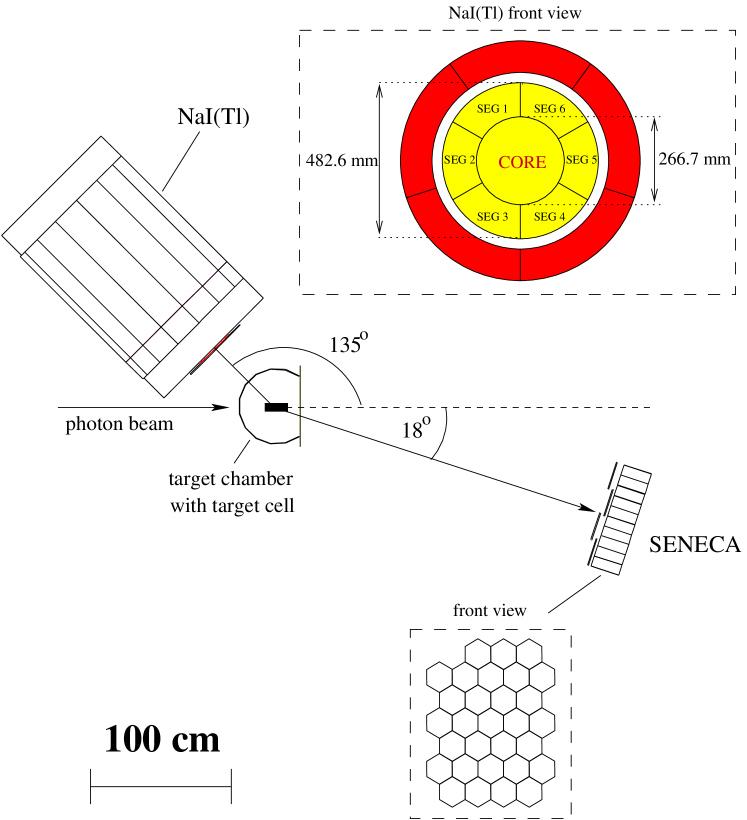
Figure 1: The experimental setup used to measure quasi-free Compton scattering from the bound neutron and proton. The scattered photons were detected with the large volume NaI(Tl) detector, the recoiling neutrons and protons with the SENECA detector system. Liquid deuterium and liquid hydrogen have been used as target materials. The target cells are mounted in a scattering chamber having a Kapton window downstream the photon beam to reduce the energy loss of the protons on their way to SENECA.

SENECA was built as a neutron detector capable of pulse-shape discrimination. It consists of 30 hexagonally shaped cells filled with NE213 liquid scintillator (15 cm in diameter and 20 cm in length) mounted in a honeycomb structure. Originally, this detector was designed for neutrons with energies up to 50 MeV. Because of the considerably higher neutron energies, in the present experiment pulse-shape discrimination was not of an essential help. Nevertheless, the detector had ideal properties for the present application, mainly because of its high granularity and because the shape of the detector modules is favorable for computer simulations and detection-efficiency measurements. Veto-detectors in front of SENECA provided the possibility to identify charged background particles and to discriminate between neutrons and protons. This allowed clean separation between quasi-free Compton scattering and $\pi^{0}$ photoproduction from the proton and neutron detected in the same experiment. The detection efficiency of the veto-detectors for protons was implemented in the Monte Carlo program and determined from the free-proton experiment by making use of the large amount of $\pi^{0}$ photoproduction data. The detection efficiency was found to be 99 % in close agreement with the predictions of the Monte Carlo program.

The momenta of the recoil nucleons were measured using the time-of-flight (TOF) technique with the NaI(Tl) detector providing the start signal and the SENECA modules providing the stop signals. For that purpose each SENECA module had to be time calibrated relative to the NaI(Tl) detector and this was carried out in two steps. First, the veto-detector in front of the NaI(Tl) detector was time calibrated relative to the NaI(Tl) detector. Thereafter, this veto-detector was mounted underneath the SENECA detector so that cosmic-ray muons could be used for the time calibration of the SENECA modules relative to the veto-detector. Walk corrections of the detectors were performed by measuring time differences relative to the tagger signal as a function of pulse height.

Data were collected during 238 h of beam time with a deuterium target. In a separate run of 35 h the same target cell was filled with liquid hydrogen in order to measure Compton scattering from the free proton at exactly the same kinematical conditions. These latter data were also used to measure the neutron detection efficiency of SENECA as described in subsection 3.3. The tagging efficiency, being 55 %, was measured several times during the runs by means of a Pb-glass detector moved into the direct photon beam, and otherwise monitored by a P2-type ionization chamber positioned at the end of the photon beam line.

3 Data analysis

3.1 Identification of $(\gamma,\gamma)$ and $(\gamma,\pi^{0})$ events

Before analysing the data obtained with the deuterium target the corresponding analysis of data obtained with the hydrogen target was carried out. In this case the separation of events from Compton scattering and $\pi^{0}$ photoproduction can be achieved by the NaI(Tl) detector alone, but the detection of the recoiling proton improves the separation, especially for energies near the peak of the $\Delta$ resonance. A typical spectrum is shown in panel a of Fig. 2. The data obtained for the free proton have been used to optimize the analysis procedure for the bound nucleon described in the following.

The time-of-flight measured for protons is modified through energy losses in the target and in the materials between target and the SENECA modules. The necessary correction was carried out through an iteration. Starting with an estimated kinetic energy of the proton, the energy loss was calculated in steps of a few mm in all materials traversed by the proton. To achieve good precision in a minimum of computer time, the step size was chosen to depend on the material. The calculated TOF thus achieved was compared with the measured one. In case of a difference the estimated initial energy of the proton was modified and the TOF was calculated again. By this procedure the initial kinetic energy of the proton was found after few iterations. Except for the energy loss and a slightly different effect of the spatial resolution of the SENECA modules, the kinetic energy of the recoiling neutrons was determined in the same way.

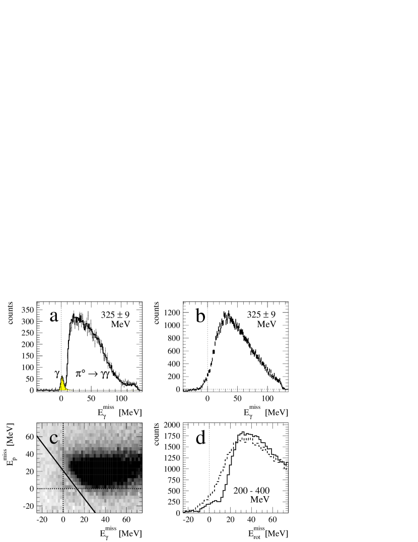
Figure 2: Panel a: Number of proton events obtained with a hydrogen target versus the missing photon energy $E^{\rm miss}_{\gamma}$. Panel b: The same as panel a but for proton events obtained with a deuterium target. Panel c: Scatter plot of proton events obtained with a deuterium target. Abscissa and ordinate are the missing energies of the scattered photon and the recoil proton, respectively. The thick solid line separates Compton events located in the vicinity of the origin of the coordinate system and $(\gamma,\pi^{0})$ events shown as a dark range. For the further evaluation each point in the scatter plot was rotated (moved on a circle centered at the origin), until the thick solid line was perpendicular to the abscissa. Panel d: Projection of proton events obtained with a deuteron target after rotation (solid line) and before rotation (broken line).

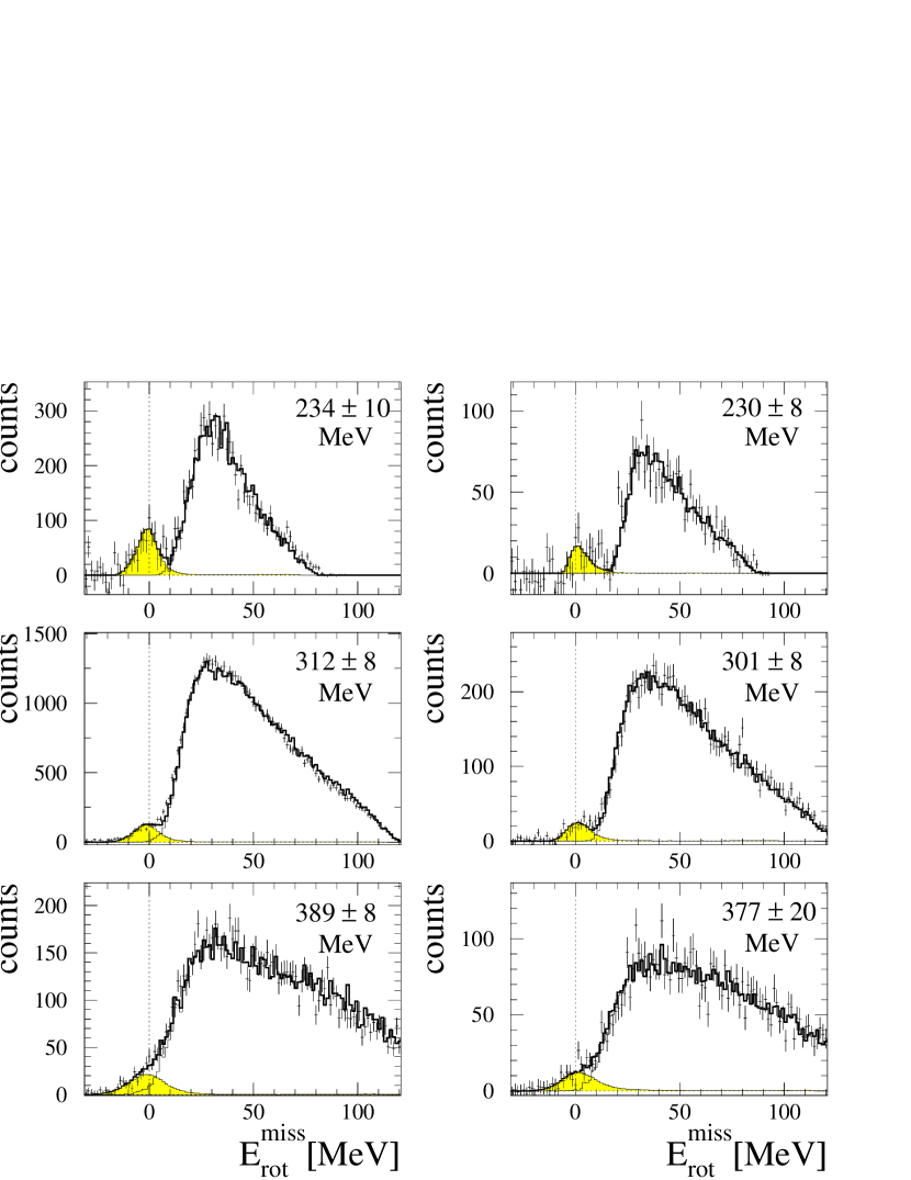
Figure 3: Typical spectra of events obtained with the deuteron target shown for the recoil proton (left panels) and recoil neutrons (right panels). The data from the two dimensional plot have been projected on the abscissa after the rotation described in the caption of Fig.2 and in the text has been carried out. The solid curves are the results of a Monte Carlo simulation scaled to the Compton events and the $(\gamma,\pi^{0})$ events, respectively.

For the separation of events from Compton scattering and $\pi^{0}$ photoproduction it is convenient to use two-dimensional scatter plots of events with the missing nucleon energy $E^{\rm miss}_{N}=E^{\rm calc}_{N}-E^{\rm SEN}_{N}$ and the missing photon energy $E^{\rm miss}_{\gamma}=E^{\rm calc}_{\gamma}-E^{\rm NaI}_{\gamma}$ as the parameters, where $E^{\rm SEN}_{N}$ and $E^{\rm NaI}_{\gamma}$ denote measured energies and $E^{\rm calc}_{N}$ and $E^{\rm calc}_{\gamma}$ the corresponding calculated energies. The calculations are carried out using the tagged photon energy and the detected nucleon angle or scattered photon angle and assuming the kinematics of Compton scattering by the proton in case of a hydrogen target or the kinematics of Compton scattering in the center of the quasi-free peak levchuk94 in case of a deuteron target. As an example, the panel c of Fig. 2 shows the scatter plot of proton events obtained with 200 MeV $-$ 400 MeV photons incident on a deuterium target. Two separate regions containing events are visible. The Compton events are located in a narrow zone around the origin ($E^{\rm miss}_{\gamma}=0,E^{\rm miss}_{p}=0$), the $(\gamma,\pi^{0})$ events in the dark range at larger missing energies. For the further evaluation each point in the panel was rotated (moved on a circle centered in the origin) until the thick solid line became perpendicular to the abscissa. This has the advantage that projections of the data on the new abscissa – denoted by $E^{\rm miss}_{\rm rot}$ – can be used for the further analysis without essential loss in the quality of separation of the two types of events.

The benefits of this procedure are illustrated in Fig. 2. Panel a shows numbers of proton events from a proton target versus the measured missing energy of the scattered photon, given for a narrow energy interval close to the maximum of the $\Delta$-resonance. In this case we find a very good separation of the two types of events as in previous experiments carried out with proton targets. The good separation disappears when proton events of the same type are taken from a deuteron target. These data are shown in panel b, where it can clearly be seen that the effects of binding destroy the separation of the two types of events which was visible in panel a. The separation can be partly restored when the rotation procedure is applied, as is shown in panel d. This panel contains as a solid line the same data as the scatter plot of events shown in panel c but projected on the abscissa after rotation. For comparison the broken line shows the same data before rotation. The comparison of these two lines clearly demonstrates that the rotation procedure essentially improves on the separation of the two types of events. In principle it also would have been possible to use the two dimensional scatter plot directly for the separation. However, this latter procedure would have been difficult because of the limited statistical accuracy which is even less favorable for the case of neutron events.

Figure 3 shows typical spectra obtained with the deuterium target. The left panels contain proton events, the right panels neutron events. The different numbers of events on the two sides are due to the neutron detection efficiency which was 18 %. As expected from the findings of panel d of Fig. 2, there is a reasonable separation of the two types of events in the whole energy range. For the final separation and for the determination of the numbers of Compton events, a complete Monte Carlo simulation has been carried out for the processes under consideration. In order to achieve high precision, all details of the experiment were implemented with great care. The results of these simulations shown by solid curves were scaled to the Compton and $(\gamma,\pi^{0})$ data, thus leading to the grey areas in case of the Compton scattering events and to the white areas in case of the $\pi^{0}$ events.

3.2 Details of Monte Carlo simulations and differential cross sections

3.2.1 Compton scattering by the free proton

In case of the free proton (hydrogen target), the differential cross section is given by the number of scattered photons, the incident photon flux and the solid angle of the NaI(Tl) detector. The determination of the latter needs a rather detailed Monte Carlo simulation of the exact experimental setup including target position, beam profile and all detector materials and resolutions. The simulation is based on the package GEANT provided by the CERN computing department brun93 . The event generator uses the angular and energy distributions for Compton scattering calculated with the dispersion approach by L’vov et al. LPS97 .

Since there is a large component due to $\pi^{0}$ photoproduction in the missing-energy spectra, also this process has to be included in the simulation. For free $\pi^{0}$ photoproduction, the angular and energy distributions were calculated using the SAID partial wave analysis arndt96 ; said .

For both Compton scattering and $\pi^{0}$ photoproduction from the free proton the missing-energy spectra, like the one shown in Fig. 2 panel a, show very good agreement between the measured and simulated spectra after the scaling to the experimental data has been carried out. Therefore, the experimental setup is well described in our Monte Carlo program. Comparing the measured and simulated spectra gives the number of scattered photons. Differential cross sections are then obtained by normalizing to the number of target nuclei and to the incident photon flux.

3.2.2 Quasi-free Compton scattering by the nucleon

In case of quasi-free Compton scattering and $\pi^{0}$ photoproduction, the aim of the analysis is to determine the triple differential cross section in the center of the quasi-free peak. For this purpose the Monto-Carlo simulation as described above has to be extended in order to also include the effects of the quasi-free reactions. For quasi-free Compton scattering the theoretical treatment of levchuk94 ; wissmann98 was used for this purpose whereas quasi-free $\pi^{0}$ photoproduction was based on the treatment given in LLP96 . The events have to be distributed along all possible kinematical variables since they are only strongly correlated in the center of the quasi-free peak. After all variables were selected for a Monte Carlo event the weight of such an event was determined according to the theoretical cross section. The geometrical boundary conditions set by the acceptances of the detectors were sufficiently enlarged in order to make sure that the final sample of Monte Carlo events was complete. The agreement between experiment and simulation is demonstrated in Fig. 3 and has already been discussed in the previous section.

The number of Compton scattered events, which is the number of events as given by the adjusted curves, corresponds to the integral of the triple differential cross section in the region of the quasi-free peak. The following relation has been used to determine the final triple differential cross section in the center of the nucleon quasi-free peak (NQFP):

$$\left(\frac{d^{3}\sigma}{{d\Omega_{\gamma}}{d\Omega_{N}}{dE_{N}}}\right)_{NQFP}=\frac{N_{\gamma N}}{N_{\gamma}N_{T}\epsilon_{N}R^{\gamma\gamma}_{NQFP}}\;,$$ (12)

where $N_{\gamma N}$ are the number of coincident $\gamma$-nucleon events as extracted from the missing-energy spectra, $N_{\gamma}$ are the number of incident photons, $N_{T}$ are the number of target nuclei, $\epsilon_{N}$ is the nucleon detection efficiency and $R^{\gamma\gamma}_{\rm NQFP}$ is a factor obtained by a Monte Carlo simulation which relates the number of scattered photons integrated over the Compton peak to the triple differential cross section in the center of the nucleon quasi-free peak.

3.3 Neutron detection efficiency

The neutron detection efficiency can be determined experimentally using neutrons from the reaction $p(\gamma,\pi^{+}n)$ on the free proton, with the $\pi^{+}$ meson detected by the NaI(Tl) detector and identified as a charged particle by the veto-counter in front of it. The NaI(Tl) detector measures the kinetic energy of the $\pi^{+}$ meson, so that after the necessary corrections for energy losses in the materials on the way from the production point to the NaI(Tl) detector are carried out, the experimental initial kinetic energy $E_{\pi^{+}}^{\text{NaI}}$ at the reaction point is known. The same quantity can also be calculated from the incident photon energy and the $\pi^{+}$ emission angle, leading to $E_{\pi^{+}}^{\text{calc}}$. From these two values for the $\pi^{+}$ energy, the missing $\pi^{+}$-energy

$$E_{\pi^{+}}^{\text{miss}}=E_{\pi^{+}}^{\text{calc}}-E_{\pi^{+}}^{\text{NaI}},$$ (13)

can be calculated and used for the identification of a
$p(\gamma,\pi^{+}n)$ event.

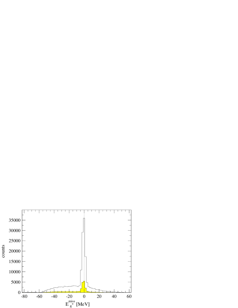
Figure 4: Missing kinetic energy of the $\pi^{+}$ meson from the reaction $p(\gamma,\pi^{+})$ with the $\pi^{0}$ meson detected by the NaI(Tl) detector (solid line) and the same data as obtained in coincidence with a neutron identified with SENECA (grey area).

The spectrum of events versus the missing energy as shown in Fig. 4 has the expected structure with a narrow peak around zero missing energy containing the cleanly identified $p(\gamma,\pi^{+}n)$ events on top of a broad background.

Since the kinematical quantities are fixed through the $\pi^{+}$ meson spectrometrized by the NaI(Tl) detector, the corresponding recoiling neutron will hit the SENECA detector. Therefore, the same missing energy spectrum is obtained in coincidence with the SENECA detector, except for a factor which is equal to the neutron detection efficiency $\epsilon_{n}$. The coincidence spectrum is shown by the grey area in Fig. 4. The result of the present measurement is represented in Fig. 5 by filled circles. It is obvious that the present data have comparatively small errors and, therefore, largely reduce the uncertainties in the neutron detection efficiencies $\epsilon_{n}$ contained in previous measurements, obtained with monoenergetic neutrons at the Paul-Scherrer-Institute (Villigen, Switzerland) edel92 , at the Physikalisch-Technische Bundesanstalt (Braunschweig, Germany) edel92 ; gall93 and at the electron accelerator ELSA (Bonn, Germany) maas95 . For the simulation the code GCALOR zeit96 was available which realistically takes into acount the interaction of neutrons and charged pions with the materials down to energies of $\sim$ 1 MeV. This program, however, requires very much computer time. Therefore, the much faster Gamma-Hadron-Electron-Interaction SH(A)ower code GHEISHA fese85 was used which is included in GEANT as a standard. Uncertainties contained in this latter code were eliminated by correcting the simulated results with the ratio of the results of the present experiment and the simulation.

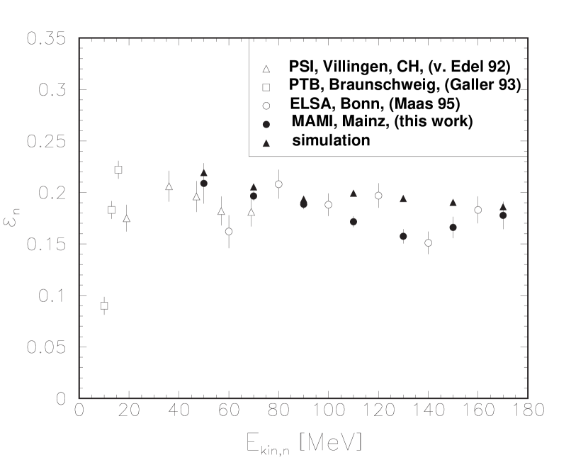
Figure 5: The neutron detection efficiency of SENECA as measured in the present experiment via the reaction $p(\gamma,\pi^{+}n)$ (full circles).

4 Theory

4.1 Definition of electromagnetic polarizabilities

Following lvov93 we define the electric polarizability $\alpha$ and the magnetic polarizability $\beta$ through the relations

$${\bf D} = 4\pi\,\alpha\,{\bf E},$$ (14)

$${\bf M} = 4\pi\,\beta\,{\bf H},$$ (15)

$$V_{\rm pol}(\alpha,\beta) = -\frac{1}{2}(4\pi\,\alpha)\,{\bf E}^{2}-\frac{1}{2}(4\pi\,\beta)\,{\bf H}^{2}.$$ (16)

In (14) – (16) ${\bf E}$ and ${\bf H}$ are the electric and magnetic fields, respectively, ${\bf D}$ and ${\bf M}$ the induced electric and magnetic dipole moments, respectively, and $V_{\rm pol}$ is the polarization potential. The factors $4\pi$ introduced in (14) – (16) indicate that electromagnetic polarizabilities are traditionally given in Gaussian units. The same quantities $\alpha$ and $\beta$ also enter into the amplitude for Compton scattering up to the order ${\cal O}(\omega^{2})$

$$T=T_{\rm Born}+\omega\omega^{\prime}\alpha{\boldsymbol{\epsilon}}\cdot{\boldsymbol{\epsilon}}^{\prime}+\omega\omega^{\prime}\beta{\bf s}\cdot{\bf s}^{\prime}+{\cal O}(\omega^{3})$$ (17)

and into the differential cross section for electromagnetic scattering of slow neutrons in the Coulomb field of heavy nuclei

$$\frac{d\sigma_{\rm pol}}{d\Omega}=\pi Mp(Ze)^{2}{\rm Re}a\left\{\alpha_{n}\sin\frac{\theta}{2}-\frac{e^{2}\kappa^{2}_{n}}{2M^{3}}\left(1-\sin\frac{\theta}{2}\right)\right\}.$$ (18)

In (17) $T_{\rm Born}$ denotes the Born amplitude and ${\boldsymbol{\epsilon}}$, ${\boldsymbol{\epsilon}}^{\prime}$ the unit vectors in the directions of the electric fields of the ingoing and outgoing photons, respectively, and ${\bf s}$ and ${\bf s}^{\prime}$ the corresponding unit vectors for the magnetic fields. In (18) $p$ is the neutron momentum and $-a$ the amplitude for hadronic scattering by the nucleus. The second term in the braces is due to the Schwinger term, i.e. the term describing neutron scattering in the Coulomb field due to the magnetic moment only. As outlined in the introduction, this part of the scattering differential cross section has been omitted in previous evaluations of neutron transmission experiments. Therefore, the results of those experiments have to be corrected by increasing them by $e^{2}\kappa^{2}_{n}/4M^{3}=0.62$.

In some treatments the electromagnetic polarizabilities entering into (17) and (18) are denoted by $\bar{\alpha}$ and $\bar{\beta}$ in order to descriminate them from the quantities entering into (14) – (16). However, since these quantities are identical lvov93 , there is no good reason for using different notations.

4.2 Non-subtracted fixed-$t$ dispersion theory

The low-energy expansion of the Compton scattering amplitude (17) is valid up to photon energies of about 100 MeV. Even with terms $\sim{\cal{O}}(\omega^{4})$ included the amplitude can be used only below pion photoproduction threshold. It has been shown experimentally lara01 ; wolf01 that the fixed-$t$ dispersion theory as constructed in LPS97 is valid up to photon energies of about 800 MeV. Therefore, an appropriate procedure to overcome the limitations inherent in (17) is to apply fixed-$t$ dispersion theory in its general form and to adjust its predictions to experimental Compton scattering data in angular and energy regions where the sensitivity of the differential cross section to the quantity under consideration is strong.

In the general case Compton scattering is described by six invariant amplitudes $A_{i}(\nu,t)$, $i=1\cdots 6$ where

$$\nu = \frac{s-u}{4m}=E_{\gamma}+\frac{t}{4m},\quad t=(k-k^{\prime})^{2},\quad s=(k+p)^{2},$$

$$u = (k-p^{\prime})^{2}$$ (19)

and $s+u+t=2m^{2}$, with $m$ being the nucleon mass. These amplitudes can be constructed to have no kinematical singularities and constraints and to obey the usual dispersion relations. In LPS97 fixed-$t$ dispersion relations for $A_{i}(\nu,t)$ were formulated by using a Cauchy loop of finite size (a closed semicircle of radius $\nu_{max}$), so that LPS97

$${\rm Re}A_{i}(\nu,t)=A^{\rm pole}_{i}(\nu,t)+A^{\rm int}_{i}(\nu,t)+A^{\rm as}_{i}(\nu,t)$$ (20)

with

$$A^{\rm pole}_{i}(\nu,t) = \frac{a_{i}(t)}{\nu^{2}-t^{2}/16m^{2}},$$

$$A^{int}_{i}(\nu,t) = \frac{2}{\pi}{\cal P}\int^{\nu_{\rm max}(t)}_{\nu_{\rm thr}(t)}{\rm Im}A_{i}(\nu^{\prime},t)\frac{\nu^{\prime}d\nu^{\prime}}{\nu^{\prime 2}-\nu^{2}},$$

$$A^{\rm as}_{i}(\nu,t) = \frac{1}{\pi}{\rm Im}\int_{{\cal C}_{\nu_{\rm max}}}A_{i}(\nu^{\prime},t)\frac{\nu^{\prime}d\nu^{\prime}}{\nu^{\prime 2}-\nu^{2}}.$$ (21)

The explicit use of the contour integral for $A^{\rm as}(\nu,t)$ is only necessary for i = 1 and 2, where special models have to be used for this purpose. For i = 3 $\cdots$ 6 the contour integral for $A^{\rm as}(\nu,t)$ can be avoided by extending the integral for $A^{int}(\nu,t)$ to infinity.

The integral contributions $A^{\rm int}_{i}(\nu,t)$ are determined by the imaginary part of the Compton scattering amplitude which is given by the unitarity relation of the generic form

$$2{\rm Im}T_{fi}=\sum_{n}(2\pi)^{4}\delta^{4}(P_{n}-P_{i})T^{*}_{nf}T_{ni}.$$ (22)

The quantities entering into the r.h.s. of (22) are from $|n\rangle=|\pi N\rangle$ and $|n\rangle=|2\pi N\rangle$ intermediate states where the $|n\rangle=|\pi N\rangle$ component can be constructed from recent parametrizations (SAID arndt96 ; said and MAID drechsel99 ; maid ) of pion photoproduction multipoles $E_{l\pm}$, $M_{l\pm}$. The $|n\rangle=|2\pi N\rangle$ component requires additional model considerations LPS97 .

For the asymptotic ($t-$channel) part of the amplitude $A_{2}(\nu,t)$ we may use the Low amplitude of $\pi^{0}$ exchange in the $t-$channel, supplemented by $\eta$ and $\eta^{\prime}$ exchanges:

$$A^{\rm as}_{2}(t)=A^{\pi^{0}}_{2}(t)+A^{\eta}_{2}(t)+A^{\eta^{\prime}}_{2}(t)$$ (23)

with

$$A^{\pi^{0}}_{2}(t)=\frac{g_{\pi NN}F_{\pi^{0}\gamma\gamma}}{t-m^{2}_{\pi^{0}}}\tau_{3}F_{\pi}(t),$$ (24)

where the isospin factor is $\tau_{3}=\pm 1$ for the proton and neutron, respectively, and the product of the $\pi NN$ and $\pi^{0}\gamma\gamma$ couplings is LPS97

$$g_{\pi NN}F_{\pi^{0}\gamma\gamma} = -16\pi\sqrt{\frac{g^{2}_{\pi NN}}{4\pi}\frac{\Gamma_{\pi^{0}\to 2\gamma}}{m^{3}_{\pi^{0}}}}$$ (25)

$$= (-0.331\pm 0.012)\,{\rm GeV}^{-1}.$$

The comparatively small contributions due to the $\eta$ and $\eta^{\prime}$ mesons are constructed in analogy to the term representing the $\pi^{0}$ contribution.

In the frame of the invariant amplitudes, the backward spin polarizability $\gamma_{\pi}$ is given by

$$\gamma_{\pi}=-\frac{1}{2\pi m}\left[A^{\rm int}_{2}(0,0)+A^{\rm as}_{2}(0,0)+A^{\rm int}_{5}(0,0)\right]$$ (26)

with the integral ($s-$channel) part being the smaller contribution.

There have been arguments tonnison98 ; blanp01 that $A^{\rm as}_{2}(t)$ is not exhausted by $\pi^{0}$, $\eta$ and $\eta^{\prime}$ exchanges in the $t-$channel. In order to introduce an additional parameter into the relevant amplitude which provides the necessary flexibility for an experimental test, we use the replacement

$$A^{\rm as}_{2}(t)\to A^{\rm as}_{2}(t)-2\pi m\frac{\delta_{\gamma_{\pi}}}{1-\frac{t}{\Lambda^{2}}}$$ (27)

from which the substitution follows:

$$\gamma_{\pi}\rightarrow\gamma_{\pi}+\delta\gamma_{\pi}.$$ (28)

The cutoff parameter $\Lambda$ of the monopole form factor defines the slope of the function at $t=0$ and is chosen to be $\Lambda=700$ MeV, as estimated from the axial radius of the nucleon and the size of the pion LPS97 . In varying $\delta\gamma_{\pi}$ the influence of any deviation from the standard value of $\gamma_{\pi}$ can be investigated in terms of this ansatz. It should be noted that this procedure is completely decoupled from the choice of the parametrization of the photo-meson amplitudes $E_{l\pm}$ and $M_{l\pm}$.

Instead of calculating the $s-$channel part of $\gamma_{\pi}$ from the integral amplitudes $A^{\rm int}_{2}(0,0)$ and $A^{\rm int}_{5}(0,0)$ of (26) the sum rule derived in lvov99 may be used for this purpose:

$$\gamma_{\pi}(s-{\rm{channel}}) =\int^{\infty}_{\omega_{0}}\sqrt{1+\frac{2\omega}{m}}\left(1+\frac{\omega}{m}\right)$$ (29)

$$\times\sum_{n}P_{n}[\sigma^{n}_{3/2}-\sigma^{n}_{1/2}]\frac{d\omega}{4\pi^{2}\omega^{3}}$$

where $\sigma^{n}_{\lambda}$ is the photoabsorption cross section with specific total helicity $\lambda$ of the beam and target and with relative parity $P_{n}=\pm 1$ of the final state $n$ with respect to the target.

The asymptotic contribution of the amplitude $A_{1}(\nu,t)$ is modeled through an ansatz analogous to the Low amplitude, except for the fact that the pseudoscalar meson $\pi^{0}$ is replaced by the scalar $\sigma$-meson. In this case we use a simpler form of the ansatz

$$A^{\rm as}_{1}(t)\simeq A^{\sigma}_{1}(t)=\frac{g_{\sigma NN}F_{\sigma\gamma\gamma}}{t-m^{2}_{\sigma}}$$ (30)

and include quantities like the formfactor in (24) into the ”effective mass” $m_{\sigma}$ being now an adjustable parameter LPS97 . The quantity $g_{\sigma NN}F_{\sigma\gamma\gamma}$ is given by the difference of the electric and magnetic polarizabilities $\alpha--\beta$ through

$$2\pi(\alpha-\beta)+A^{\rm int}_{1}(0,0)=-A^{\rm as}_{1}(0,0)=\frac{g_{\sigma NN}F_{\sigma\gamma\gamma}}{m^{2}_{\sigma}}$$ (31)

with the integral part being a minor contribution. The quantity $m_{\sigma}$ has a strong impact on the differential cross section in the 400 to 700 MeV energy region and has been determined experimentally to be $m_{\sigma}\approx 600$ MeV lara01 ; wolf01 .

For the proton $\alpha_{p}-\beta_{p}$ has been determined in a series of Compton scattering experiments carried out below $\pi$ photoproduction threshold. The results may be summarized by quoting the global average olmos01 $\alpha_{p}-\beta_{p}=10.5\pm 0.9({\rm stat+syst})\pm 0.7({\rm model})$. Adopting this value, the correction $\delta\gamma_{\pi}$ introduced in (28) has been determined to be comparable with $\delta\gamma^{(p)}_{\pi}=0$ camen02 .

In the present experiment $\alpha_{n}-\beta_{n}$ will be determined from experimental differential cross sections measured at energies above $\pi$ threshold. This strongly reduces the possibility to disentangle the determination of $\alpha_{n}-\beta_{n}$ and $\gamma^{(n)}_{\pi}$. Our procedure, therefore, is to assume that the result $\delta\gamma_{\pi}=0$ obtained for the proton is also true for the neutron and then to extract $\alpha_{n}-\beta_{n}$ from fits to the experimental data. This point will be discussed in more detail later.

4.3 Quasi-free Compton scattering

A calculation of the reaction $\gamma d\to\gamma^{\prime}np$ has been carried out in Ref. levchuk94 (see also Ref. wissmann98 ) in the framework of a diagrammatic approach. The main graphs contributing to the reaction amplitude in the quasi-free region are displayed in Fig. 6. Graphs 6a) and b) describe quasi-free scattering from the neutron and proton, respectively. The non-interacting nucleon in these graphs is often referred to as a spectator. Nucleon-nucleon rescattering (or final state interaction, FSI) shown in graphs 6c) and d), as well as meson seagull contributions and isobar configurations described by graphs 6e) and f) have also been taken into account.

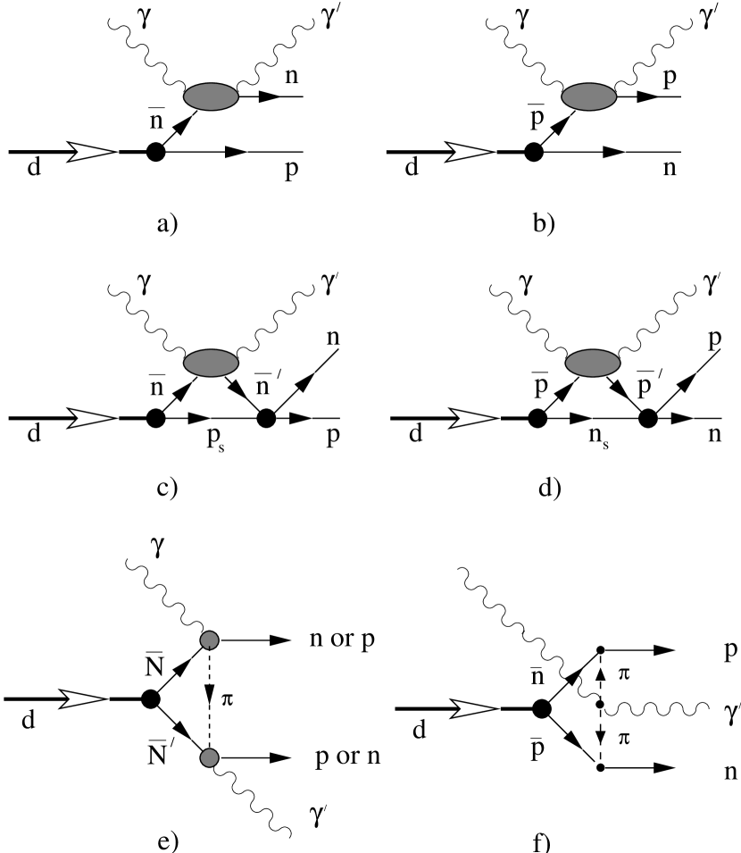
Figure 6: Main graphs contributing to the reaction $\gamma d\to\gamma^{\prime}np$. The shaded areas in graph e) stand for the $\gamma N\to\pi N$ and $\pi N\to\gamma N$ amplitudes including pole and $\Delta$ terms.

All the details of the calculations can be found in Ref. levchuk94 . Here we mention only the following. A model of $NN$-interaction is needed to calculate the deuteron wave function and the $NN$-scattering amplitude when evaluating the diagrams. We checked three versions of the Bonn OBEPR model OBEPR1 ; OBEPR2 , CD-Bonn potential CD-Bonn , and a separable approximation PEST1 ; PEST2 of the Paris potential Paris . Our observation is that the results obtained with all the Bonn potentials are practically the same so that in the following we will present our results with the CD-Bonn and Paris models only. One more important ingredient of the model is the nucleon Compton scattering amplitude. It enters the graphs in Fig. 6a)-d). This amplitude is taken from the currently accepted dispersion model LPS97 which provides a satisfactory description of all available data on free proton Compton scattering up to 800 MeV lara01 ; wolf01 . As an input of the model the amplitudes of single pion photoproduction are used. In the present work they are taken from the SAID arndt96 ; said (solutions SM99K and SM00K) and MAID drechsel99 ; maid (solution MAID2000) analyses. Of course when considering the diagrams 6a)-d) we have to deal with off-shell nucleons. The off-shell corrections, however, are expected to be very small in the kinematic conditions under consideration (see a discussion in Ref. levchuk94 ) so that the use of the on-shell parametrization for the nucleon Compton scattering amplitudes is quite justified.

The measured triple differential cross section,
$d^{3}\sigma/d\Omega_{\gamma^{\prime}}d\Omega_{p}dE_{p}$ (here $E_{p}$ and $\Omega_{p}$ are the kinetic energy and solid angle of the proton), in the center of the proton quasi-free peak (pQFP) can be related to the free differential cross section, $d\sigma/d\Omega_{\gamma^{\prime}}$, via a spectator formula levchuk94 ; wissmann99

$$\frac{d\sigma(\gamma p\rightarrow\gamma^{\prime}p)}{d\Omega_{\gamma^{\prime}}}=\frac{(2\pi)^{3}}{u^{2}(0)}\frac{E_{\gamma}E_{\gamma^{\prime}}}{|{\bf p}|m{E_{\gamma^{\prime}}^{(p)2}}}\frac{d^{3}\sigma(\gamma d\rightarrow\gamma^{\prime}pn)}{d\Omega_{\gamma^{\prime}}d\Omega_{p}dE_{p}},$$ (32)

where $u(0)$ is the S-wave amplitude of the deuteron wave function at zero momentum (the D-wave component of this function does not contribute at zero momentum), $E_{\gamma^{\prime}}^{(p)}=(p_{\gamma^{\prime}}\!\!\cdot p_{p})/m$ is the final photon energy in the rest frame of the final proton and ${\bf p}$ is the momentum of the final proton. In case of neutron quasi-free scattering, one has an analogous formula with the replacement $p\leftrightarrow n$. Note that there is a slight dependence of the factor
$(2\pi)^{3}/u^{2}(0)$ in the r.h.s. of Eq. (32) on the model of $NN$-interaction. For instance, this factor is equal to $592055\,\mathrm{MeV^{3}}$ and $599089\,\mathrm{MeV^{3}}$ for the CD-Bonn and for the Paris potential, respectively, i.e., it varies within 1.2 %.

Equation (32) is valid for the pole diagram contribution only. Therefore, for the measured cross section to be used in Eq. (32) the r.h.s. of this equation has to be multiplied by a factor $f(E_{\gamma},\theta_{\gamma})=d^{3}\sigma_{pol}/d^{3}\sigma_{tot}$. Here, $d^{3}\sigma_{pol}$ stands for the contribution of the pole (proton or neutron) diagram to the total differential cross section $d^{3}\sigma_{tot}$ for which all the diagrams a)-f) have been taken into account. The difference $1-f$ shows the relative contribution of the background effects which are mainly from FSI and ranges in the center of the pQFP at $\theta^{\rm LAB}_{\gamma}=136.2^{\circ}$ from $-0.049$ at 234 MeV to $-0.014$ at 389 MeV for the CD-Bonn potential and from $-0.054$ to $-0.024$ for the Paris one. In the center of the neutron quasi-free peak (nQFP) at the same angle this factor varies from $-0.081$ at 211 MeV to $-0.013$ at 377 MeV for the CD-Bonn potential and from $-0.097$ to $-0.019$ for the Paris potential. The small value of the factor $1-f$ shows that the background contributions due to FSI and seagull terms are small at the relatively high photon energies and large photon angle under consideration. At energies below pion photoproduction threshold and/or for forward photon scattering the above contributions (mainly due to FSI) are much larger (see Refs. levchuk94 ; wissmann98 ).

The total factor relating the free and quasi-free cross sections ranges from 1.48 (1.52) at 210 MeV to 0.68 (0.70) at 380 MeV for CD-Bonn (Paris) potential at $\theta^{\rm LAB}_{\gamma}=136.2^{\circ}$, i.e. it has only a minor dependence on the choice of a model of $NN$-interaction. It is seen that the factor can lead to both lowering and increasing the ”free” cross section in comparison with the quasi-free cross section.

When relating the free and quasi-free cross section the effect of the deuteron binding has to be taken into account because of the rather strong energy dependence of the differential cross section. This means that the equivalent free photon energy $E^{f}_{\gamma}$ is not equal to $E_{\gamma}$ but related with it in the center of NQFP through the equation

$$E^{f}_{\gamma}=E_{\gamma}-\Delta\left(1+\frac{E_{\gamma}-\Delta/2}{m}\right),$$ (33)

where $\Delta=2.2246\,\mathrm{MeV}$ is the deuteron binding energy. Eq. (33) has a sizable effect on the construction of ”free”-nucleon differential cross sections from quasi-free triple differential cross sections.

5 Discussion of the Results

The filled circles shown in Fig. 7 represent the experimental differential cross sections obtained in the present experiment for Compton scattering by the free proton. These data are compared with predictions of the standard dispersion theory LPS97 based on different recent parametrizations of photomeson amplitudes. The curves have been obtained with a fixed value for the difference of the proton polarizabilities, $\alpha_{p}-\beta_{p}=10.5$ olmos01 . Furthermore, the standard value for the proton backward spin polarizability $\gamma^{(p)}_{\pi}=-38.7$ (in units of $10^{-4}{\rm fm}^{4}$ which will be used throughout in the following) is used without the additional contribution introduced by tonnison98 ; blanp01 for reasons discussed in camen02 . As observed before in a different recent experiment lara01 ; wolf01 there is good agreement between experiment and the predictions based on the MAID2000 and SAID-SM99K parametrizations, whereas the predictions based on the parametrization SAID-SM00K are too low in the maximum of the $\Delta$-resonance. A closer look provides us with some slight preference for the MAID2000 parametrization over the SAID-SM99K parametrization. Therefore, we base the further analysis on the MAID2000 parametrization and use the SAID-SM99K parametrization for estimates of model errors only. For comparison Fig. 7 also contains the corresponding data extracted from quasi-free Compton scattering through the model described in section 4 with (32) being the relevant formula. The results of this extraction procedure depend slightly on the choice of the $NN$-potential but are practically independent of the choice of the photomeson amplitude. Average values over the CD-Bonn and Paris models are used here. The agreement of the two types of data in Fig. 7 is good except for the two data points at 290 and 310 MeV. We consider this quality of agreement as a satisfactory justification for using the theory in the present form for the analysis of the quasi-free Compton scattering data obtained for the neutron with the residual deviations taken into account as a contribution to the model error.

Figure 8 shows the triple differential cross section for quasi-free Compton scattering. There is consistency between our data and the data point of the SAL experiment at 247 MeV.

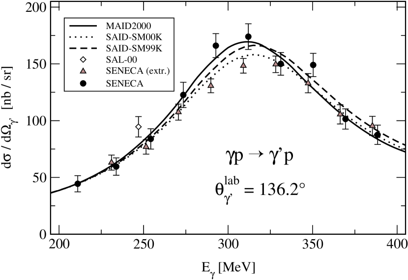
Figure 7: Differential cross sections for Compton scattering measured on a free proton (filled circles) and the corresponding data extracted from quasi-free cross sections obtained for the bound proton (grey triangles) at $\theta^{\rm LAB}_{\gamma}=136.2^{\circ}$. The SAL result kolb00 is shown by a diamond. Only statistical errors are shown. The curves were obtained using the model LPS97 for different parametrizations of photomeson amplitudes. In all curves $\alpha_{p}-\beta_{p}=10.5$ and $\gamma^{(p)}_{\pi}=-38.7$ was used.

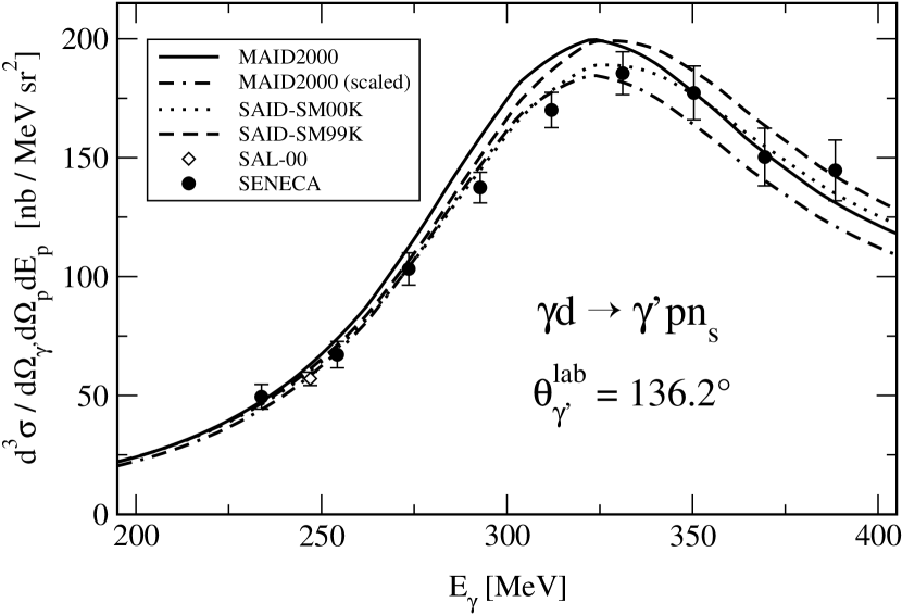
Figure 8: Triple differential cross section of the reaction $d(\gamma,\gamma^{\,\prime}p)n$ in the center of pQFP at $\theta^{\rm LAB}_{\gamma}=136.2^{\circ}$, given in the LAB frame. Circles: the present experiment; diamond: the SAL experiment kolb00 . Only statistical errors are shown. The curves were obtained using the model levchuk94 for different parametrizations of photomeson amplitudes. In all curves $\alpha_{p}-\beta_{p}=10.5$ and $\gamma^{(p)}_{\pi}=-38.7$ was used.

As expected, the triple differential cross sections of Fig. 8 reveal the same properties as the corresponding ”free” data shown in Fig. 7. The parametrizations MAID2000 and SAID-SM99K which have proven optimum for reproducing the free differential cross sections show some deviations here. At present we do not have an explanation for this deviation. Consequently, we have to treat it as a possible source of uncertainty which has to be taken into account through a further contribution to the model error. In order to get a quantitative result for this additional model error, the prediction shown in Fig. 8 as a solid curve has been scaled down by a factor of 0.93 to give the dashed-dotted curve. Through this procedure we arrive at a modified theoretical model which may be used in the further analysis to estimate the additional model error connected with a possible imperfection of the theory of quasi-free Compton scattering.

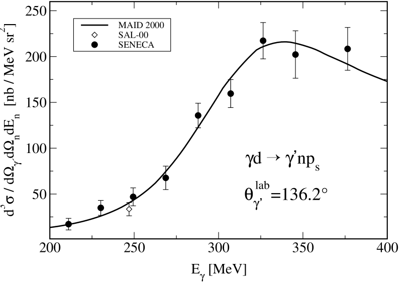
Figure 9: Triple differential cross section of the reaction $d(\gamma,\gamma^{\,\prime}n)p$ in the center of nQFP at $\theta^{\rm LAB}_{\gamma}=136.2^{\circ}$. Filled circles: the present experiment; diamond: SAL experiment kolb00 . Only statistical errors are shown. The curve was obtained in the model levchuk94 with $\gamma^{(n)}_{\pi}=58.6$ fixed and $\alpha_{n}-\beta_{n}=9.8$ determined through the fitting procedure as quoted in Eq. (34).

The measured differential cross sections for quasi-free Compton scattering are displayed in Fig. 9. Again, there is consistency with the SAL value at 247 MeV. Using the MAID2000 parametrization of photomeson amplitudes which proved to be the most favorable one in case of the free proton, we determine the polarizability difference $\alpha_{n}-\beta_{n}$ through a least-square procedure. The backward spin polarizability $\gamma^{(n)}_{\pi}=58.6$ of the neutron was used as contained in the model LPS97 for the MAID 2000 parametrization. This is justified because no indication for a deviation was found in case of the proton, i.e. $\delta^{(p)}_{\pi}=0$. The result obtained is $\alpha_{n}-\beta_{n}=9.8$ with a reduced $\chi^{2}$ of 0.6. The errors of this result are as follows. The statistical error from the $\chi^{2}$ procedure is $\pm 3.6$. The systematic error of the neutron triple differential cross sections amounts to $\pm 9\,\mathrm{\%}$, with the detection efficiency $\epsilon_{n}$ of the neutrons contributing $\pm 8\,\mathrm{\%}$, the number of target nuclei per cm² contributing $\pm 2\,\mathrm{\%}$, the uncertainties caused by cuts in the spectra and by the Monte Carlo simulations contributing $\pm 3\,\mathrm{\%}$ and the tagging efficiency contributing $\pm 2.5\,\mathrm{\%}$. For $\alpha_{n}-\beta_{n}$ this leads to a combined systematic error of ${}^{+2.1}_{-1.1}$. The model error due to imperfections of the parametrization of photomeson amplitudes was estimated from a comparison of results obtained with the MAID2000 and SAID-SM99K parametrizations. The result obtained for $\alpha_{n}-\beta_{n}$ is $\pm 2.0$. The errors due to different parametrizations of $NN$-interaction were found to be about $\pm 0.2$. The determination of the model error due to possible imperfections of the theory of quasi-free Compton scattering amounts to $\pm 0.8$.

Taking all these errors into account we obtain our final result

$$\alpha_{n}-\beta_{n}=9.8\pm 3.6\text{(stat)}\,{}^{+2.1}_{-1.1}\text{(syst)}\pm 2.2\text{(model)}.$$ (34)

Combining it with $\alpha_{n}+\beta_{n}=15.2\pm 0.5$ levc00 we obtain

$$\alpha_{n} =12.5\pm 1.8\text{(stat)}\,{}^{+1.1}_{-0.6}\text{(syst)}\pm 1.1\text{(model)},$$ (35)

$$\beta_{n} =2.7\mp 1.8\text{(stat)}\,{}^{+0.6}_{-1.1}\text{(syst)}\mp 1.1\text{(model)}.$$ (36)

For sake of completeness we present in Fig. 10 the ”free” cross section obtained from the quasi-free values using the method described above for the proton case. The consistency with the dispersion calculation LPS97 is seen.

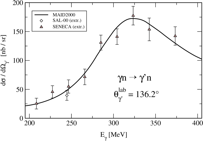
Figure 10: Differential cross sections on the ”free” neutron extracted from the quasi-free cross sections for the bound neutron at $\theta^{\rm LAB}_{\gamma}=136.2^{\circ}$ (gray triangles). The SAL result kolb00 is shown by a diamond. Only statistical errors are given. The curve was obtained in the model LPS97 using the same parameters as in Fig. 9.

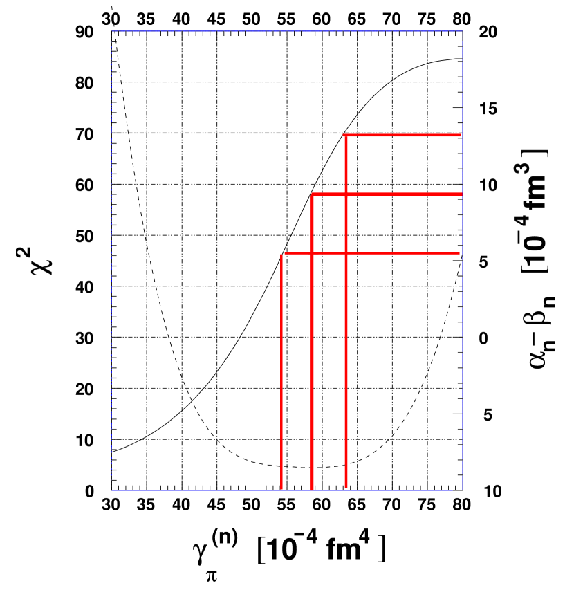
Figure 11: Solid curve: Pairs of values for $\alpha_{n}-\beta_{n}$ and $\gamma^{(n)}_{\pi}$ leading to relative best fits to the experimental triple differential cross sections for quasi-free Compton scattering by the neutron. The corresponding $\chi^{2}$ is depicted by the dashed line. The center horizontal and vertical bars correspond to the best fit obtained for $\gamma^{(n)}_{\pi}=58.6$. The outer horizontal and vertical bars correspond to the statistical errors to be attributed to the best fit.

It is of interest to compare the present results obtained for the neutron with the corresponding result for the proton. By combining the global averages of the electric and magnetic polarizabilities determined in Ref. olmos01 with the value for the sum of polarizabilities $\alpha_{p}+\beta_{p}=14.0\pm 0.3$ obtained in levc00 , we arrive at

$$\alpha_{p}=12.2\pm 0.3({\rm stat})\mp 0.4({\rm syst})\pm 0.3({\rm model}),$$ (37)

$$\beta_{p}=1.8\pm 0.4({\rm stat})\pm 0.4({\rm syst})\pm 0.4({\rm model}).$$ (38)

The backward spin polarizability for the neutron as provided by the MAID2000 parametrization through (26) is $\gamma^{(n)}_{\pi}=58.6$. For comparisons with theoretical predictions it is of interest to get some experimental information on this number. This is investigated in Fig. 11 showing the result of a least-square procedure of the same kind as used for the determination of $\alpha_{n}-\beta_{n}$. The only difference is that $\gamma^{(n)}_{\pi}$ was not kept constant at $\gamma^{(n)}_{\pi}=58.6$ but both quantities $\alpha_{n}-\beta_{n}$ and $\gamma^{(n)}_{\pi}$ were treated as free parameters. Then for each adopted value of $\gamma^{(n)}_{\pi}$ a corresponding value for $\alpha_{n}-\beta_{n}$ was obtained, with $\chi^{2}$ being at its minimum. The pairs of values for the two quantities $\gamma_{\pi}$ and $\alpha_{n}-\beta_{n}$ shown on the abscissa and the right ordinate, respectively, are depicted by a solid curve, the corresponding minimum of $\chi^{2}$ by a dashed curve. The center horizontal and vertical bars depict those pairs of $\alpha_{n}-\beta_{n}$ and $\gamma^{(n)}_{\pi}$ which correspond to the best fit to the experimental triple differential cross sections for quasi-free Compton scattering by the neutron with the spin polarizability still kept to be $\gamma^{(n)}_{\pi}=58.6$. Though the $\chi^{2}$ distribution in Figure 11 is rather broad, some information on $\gamma^{(n)}_{\pi}$ may be obtained going beyond the assumption that this quantity should be identical to the number resulting from Eq. (26). Apparently, $\gamma^{(n)}_{\pi}=58.6$ is very close to the center of the $\chi^{2}$ distribution and in this sense may be considered as being confirmed by the experiment. In order to arrive at some measure for the error of $\gamma^{(n)}_{\pi}$, we introduce in Fig. 11 the statistical error of $\alpha_{n}-\beta_{n}$ as outer horizontal bars and take the ”statistical” error of $\gamma^{(n)}_{\pi}$ from the corresponding outer vertical bars. This leads to the final result

$$\gamma^{(n)}_{\pi}=58.6\pm 4.0.$$ (39)

Table 1 summarizes the results obtained for the electromagnetic structure constants of proton and neutron in recent Compton scattering experiments. The experimental backward-angle spin polarizabilities are split up into $t-$channel and $s-$channel parts.

Table 1: Structure constants for the proton and the neutron. The quantities in lines a – c given for the neutron are from the present work, those given for the proton from our recent works olmos01 and camen02 . The numbers in lines d and f are from lvov99 . The numbers in line e are calculated from lines c and d.

structure constant	proton	neutron
$\alpha$	$12.2\pm 0.6$	$12.5\pm 2.3$	a
$\beta$	$1.8\mp 0.6$	$2.7\mp 2.3$	b
$\gamma_{\pi}$	$-38.7\pm 1.8$	$+58.6\pm 4.0$	c
$\gamma_{\pi}(t-{\rm{channel}})$	$-46.6$	$+43.4$	d
$\gamma_{\pi}(s-{\rm{channel}})$	$+7.9\pm 1.8$	$+15.2\pm 4.0$	e
$\gamma_{\pi}(s-{\rm{channel}})$	$+7.1\pm 1.8$	$+9.1\pm 1.8$	f

The $t-$channel contribution is given by the Low amplitudes of Eqs. (23) and (26), the $s-$channel contribution by the integral amplitudes $A^{\rm int}_{2}(0,0)$ and $A^{\rm int}_{5}(0,0)$ of Eq. (26). It is interesting to note that the $s-$channel contribution has a strong isovector part. This isovector part is smaller when using the sum rule of Eq. (29) for the determination of these quantities lvov99 . This simultaneously leads to a total $\gamma^{(n)}_{\pi}$ = 52.5 $\pm$ 2.4 lvov99 which hardly may be considered as consistent with the present experiment as seen in Figure 11. We tentatively assume that the large uncertainties in the photomeson amplitudes still existing in the second resonance region are responsible for this discrepancy.

Table 2: Summary on neutron polarizabilities. Lines 2 – 4 contain the results obtained by electromagnetic scattering of neutrons in a Coulomb field schmiedmayer91 , by the method of quasi-free Compton scattering above $\pi$ threshold (present work) and by coherent Compton scattering off the deuteron lundin02 .

$\alpha_{n}$+$\beta_{n}$	15.2$\pm$ 0.5	Baldin’s sum rule levc00
$\alpha_{n}$	12.6$\pm$ 2.5	Coulomb field schmiedmayer91
$\alpha_{n}$	12.5$\pm$ 2.3	quasi-free Compton (present work)
$\alpha_{n}$	9.2$\pm$ 2.2	deuteron coherent lundin02

Three independent methods for determining the electric polarizability of the neutron exist, viz. the electromagnetic scattering of neutrons in the Coulomb field of heavy nuclei, the quasi-free Compton scattering off neutrons bound in the deuteron and coherent Compton scattering by the deuteron. Table 2 contains one representative result for each method. In case of electromagnetic scattering of neutrons in a Coulomb field the result was selected where the highest precision was claimed by the authors. For coherent Compton scattering by the deuteron the most recent experiment has been selected. It appears that the three results are of comparable precision and are in agreement with each other within a 1-$\sigma$ error. However, a closer look reveals that this agreement may be fortuitous because of large uncertainties possibly contained in the results of lines 2 and 4, as discussed above. Therefore, only the present experiment where all possible errors have been analysed with great care may be considered as reliable.

The obtained value for $\alpha_{n}$ is consistent with ChPT prediction at ${\cal O}(q^{4})$ BKM95 , $\alpha_{n}=13.4\pm 1.5$, but for $\beta_{n}$ one has a noticeable disagreement, $\beta_{n}=7.8\pm 3.6$. The most recent results in the framework of heavy baryon ChPT with the $\Delta$ isobar included hemmert98 , $\alpha_{n}=16.4$ and $\beta_{n}=9.1$, contradict both measured values (35) and (36). Recently a covariant ”dressed $K$-matrix model” has been built kondr01 and its predictions for the dipole and spin polarizabilities of the nucleon have been given. The results for the proton are $\alpha_{p}=12.1$, $\beta_{p}=2.4$ and $\gamma^{(p)}_{\pi}(s-{\rm{channel}})=11.4$, and for the neutron $\alpha_{n}=12.7$, $\beta_{n}=1.8$ and $\gamma^{(p)}_{\pi}(s-{\rm{channel}})=11.2$. The results for $\alpha$, $\beta$ and $\gamma_{\pi}$ appear to be in reasonable agreement with the numbers given in Table 1, except for the fact that the predicted $\gamma_{\pi}$ has no isovector component.

The experimental data of the present experiment shown in Figs. 7 – 10 are also given in tabular form in the appendix.

6 Conclusion

The results of the present experiment can be summarized as follows. The energy dependence of the differential cross section for Compton scattering off the quasi-free proton and, for first time, off the quasi-free neutron has been measured in the energy region from 200 to 400 MeV. In agreement with the corresponding result for the proton, it is shown that the backward spin polarizability $\gamma^{(n)}_{\pi}$ needs no modification beyond the well known $s-$ and $t-$channel contributions. The values for the electric and magnetic polarizabilities of the neutron extracted from the neutron data are of high precision. They are partly in agreement with theoretical predictions.

7 Acknowledgements

Table 3: The energy dependence of the free-proton differential cross section at $\theta^{\rm LAB}_{\gamma}=136.2^{\circ}$. The statistical errors are given. The systematic error amounts to 4.4%.

$E_{\gamma}\left(\mathrm{MeV}\right)$	$\frac{d\sigma}{d\Omega_{\gamma}}\left(\frac{\text{nb}}{\text{sr}}\right)$
$211.1$		$44.4$	$\pm$	$7.1$
$233.8$		$59.6$	$\pm$	$7.6$
$254.3$		$83.9$	$\pm$	$8.9$
$273.5$		$122.7$	$\pm$	$11.1$
$292.7$		$166.1$	$\pm$	$10.6$
$312.0$		$174.0$	$\pm$	$11.3$
$331.2$		$150.0$	$\pm$	$10.0$
$350.4$		$149.1$	$\pm$	$10.2$
$369.4$		$101.5$	$\pm$	$8.4$
$388.5$		$87.6$	$\pm$	$8.5$
$407.4$		$83.5$	$\pm$	$8.5$
$427.3$		$58.7$	$\pm$	$7.4$
$448.3$		$54.1$	$\pm$	$7.4$
$469.0$		$55.3$	$\pm$	$8.1$

Table 4: The energy dependence of the differential cross section of ”free” proton Compton scattering extracted from quasi-free data at $\theta^{\rm LAB}_{\gamma}=136.2^{\circ}$. The statistical errors are given. The systematic error amounts to 4.4%.

$E_{\gamma}^{f}\left(\mathrm{MeV}\right)$	$\frac{d\sigma}{d\Omega_{\gamma}}\left(\frac{\text{nb}}{\text{sr}}\right)$
$231.0$		$63.7$	$\pm$	$6.7$
$251.5$		$77.7$	$\pm$	$6.5$
$270.6$		$108.7$	$\pm$	$7.2$
$289.8$		$132.1$	$\pm$	$6.2$
$309.0$		$149.9$	$\pm$	$6.6$
$328.2$		$151.2$	$\pm$	$7.4$
$347.4$		$134.4$	$\pm$	$8.6$
$366.3$		$106.6$	$\pm$	$8.6$
$385.4$		$96.4$	$\pm$	$8.6$

Table 5: The energy dependence of the triple differential cross section of the reaction $d(\gamma,\gamma^{\,\prime}p)n$ in the center of pQFP at $\theta^{\rm LAB}_{\gamma}=136.2^{\circ}$. The statistical errors are given. The systematic error amounts to 4.4%.

$E_{\gamma}\left(\mathrm{MeV}\right)$	$\left(\frac{d^{3}\sigma}{d\Omega_{\gamma}d\Omega_{p}dE_{p}}\right)^{\text{CpQFP}}\left(\frac{\text{nb}}{\text{MeV sr}^{2}}\right)$
$233.8$		$49.5$	$\pm$	$5.1$
$254.3$		$67.2$	$\pm$	$5.6$
$273.5$		$103.2$	$\pm$	$6.8$
$292.8$		$137.4$	$\pm$	$6.4$
$312.0$		$170.0$	$\pm$	$7.4$
$331.2$		$185.5$	$\pm$	$9.0$
$350.4$		$177.2$	$\pm$	$11.3$
$369.5$		$150.3$	$\pm$	$12.1$
$388.5$		$144.7$	$\pm$	$12.8$

Table 6: The energy dependence of the triple differential cross section of the reaction $d(\gamma,\gamma^{\,\prime}n)p$ in the center of nQFP at $\theta^{\rm LAB}_{\gamma}=136.2^{\circ}$. The statistical errors are given. The systematic error amounts to 9.0%.

$E_{\gamma}\left(\mathrm{MeV}\right)$	$\left(\frac{d^{3}\sigma}{d\Omega_{\gamma}d\Omega_{n}dE_{n}}\right)^{\text{CnQFP}}\left(\frac{\text{nb}}{\text{MeV sr}^{2}}\right)$
$211.1$		$17.1$	$\pm$	$6.3$
$230.2$		$34.9$	$\pm$	$8.1$
$249.4$		$46.9$	$\pm$	$9.8$
$268.7$		$67.6$	$\pm$	$12.8$
$287.9$		$135.7$	$\pm$	$13.4$
$307.2$		$159.6$	$\pm$	$15.3$
$326.4$		$217.3$	$\pm$	$19.8$
$345.6$		$202.2$	$\pm$	$25.9$
$376.5$		$208.4$	$\pm$	$23.4$

Table 7: The energy dependence of the differential cross section of free neutron Compton scattering extracted from the quasi-free data at $\theta^{\rm LAB}_{\gamma}=136.2^{\circ}$. The statistical errors are given. The systematic error amounts to 9.0%.

$E_{\gamma}^{f}\left(\mathrm{MeV}\right)$	$\frac{d\sigma}{d\Omega_{\gamma}}\left(\frac{\text{nb}}{\text{sr}}\right)$
$208.4$		$25.7$	$\pm$	$9.5$
$227.4$		$46.3$	$\pm$	$10.8$
$246.6$		$55.6$	$\pm$	$11.7$
$265.8$		$72.5$	$\pm$	$13.8$
$285.0$		$132.5$	$\pm$	$13.0$
$304.3$		$142.8$	$\pm$	$13.7$
$323.4$		$179.4$	$\pm$	$16.4$
$342.6$		$155.2$	$\pm$	$19.9$
$373.4$		$143.7$	$\pm$	$16.2$