Abstract

Several hadronic observables have been studied in central 158$A$ GeV Pb+Pb collisions using data measured by the WA98 experiment at CERN: single $\pi^{-}$ and $K^{-}$ production, as well as two- and three-pion interferometry. The Wiedemann-Heinz hydrodynamical model has been fitted to the pion spectrum, giving an estimate of the temperature and transverse flow velocity. Bose-Einstein correlations between two identified $\pi^{-}$ have been analysed as a function of $k_{T}$, using two different parameterizations. The results indicate that the source does not have a strictly boost invariant expansion or spend time in a long-lived intermediate phase. A comparison between data and a hydrodynamical based simulation shows very good agreement for the radii parameters as a function of $k_{T}$. The pion phase-space density at freeze-out has been measured and agrees well with the Tomás̆ik-Heinz model. A large pion chemical potential close to the condensation limit of $m_{\pi}$ seems to be excluded. The three-pion Bose-Einstein interferometry shows a substantial contribution of the genuine three-pion correlation, but not quite as large as expected for a fully chaotic and symmetric source.

1 Introduction

The study of single particle distributions of particles produced in heavy-ion collisions gives access to the degree of thermal and chemical equilibrium at freeze-out and allows the determination of the parameters of hydrodynamical expansion models of the source.

The spatio-temporal extension of the interaction region created in such collisions is not directly observable, but the study of Bose-Einstein interferometry between identical particles provides information on the geometry and on the dynamical evolution of the particle emission sources. In particular, the correlations between produced pions give access to the size of the homogeneity region, to the duration of emission, and to various parameters characterizing the spatial extension of the fireball [1]. In addition, by combining information from the source size in momentum-space obtained by interferometry, and from the momentum-space density provided by the single particle distributions, an average phase-space density at freeze-out can be calculated.

Compared to the two-particle correlation, the three-particle correlation can provide additional information on the chaoticity and asymmetry of the source emission [2, 3, 4]. In particular, the three-pion interference produced by a fully chaotic source is sensitive to the phase of the Fourier transform of the source emission function and, hence, to the asymmetry of the source.

In this paper, we present the analysis of single particle production, and of two- and three-pion interferometry measured in the WA98 experiment for central 158$A$ GeV ²⁰⁸Pb+²⁰⁸Pb collisions at the CERN SPS. In addition, estimates of hydrodynamical expansion model parameters, temperature and transverse flow velocity are extracted from these results.

2 Experimental setup and data processing

The CERN SPS fixed target experiment WA98 [5] combined large acceptance photon detectors with a two arm charged particle tracking spectrometer. The experimental layout is shown in Fig. 1. The 158$A$ GeV Pb beam interacted with a Pb target near the entrance of a large dipole magnet. The online trigger centrality selection used a forward calorimeter located at zero degrees and a mid-rapidity calorimeter measuring the total transverse energy in the pseudorapidity interval 3.2 $\leq$ $\eta$ $\leq$ 5.4. The results presented here have been obtained from an analysis of the complete data set. These data were taken with the most central triggers corresponding to about 10% of the minimum bias cross section of 6300 mb [6, 7], with an average of 330 participating nucleons per collision. These quantities are estimated to have an overall systematic error of less than 10%.

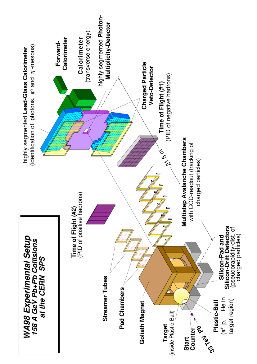
Figure 1: The WA98 experimental setup.

The charged particle spectrometer made use of a 1.6 Tm dipole magnet with a 2.4$\times$1.6 m² air gap which deflected the charged particles in the horizontal plane into two tracking arms located downstream, one on each side of the beam axis. The results shown here are measurements of $\pi^{-}$ and $K^{-}$ observed in the negative particle tracking arm of the spectrometer. This tracking arm consisted of six multistep avalanche chambers with optical readout [8]. Inside the chambers, triethylamine (TEA) photoemissive vapour produced UV photons along the path of charged particles, these photons being subsequently converted to visible light via wavelength shifter plates. On exit, the light was reflected by mirrors at 45^∘ to CCD cameras equipped with two image intensifiers. The active area of the first chamber was 1.2$\times$0.8 m² and that of the other five 1.6$\times$1.2 m². Each CCD camera pixel viewed a region of about 3.1$\times$3.1 mm² on the chambers. Downstream of the chambers, at a distance of 16.5 m from the target, a 4$\times$1.9 m² time of flight wall allowed for particle identification with a time resolution of better than 120 ps. The resulting particle separation is shown in Fig.2. The $\pi^{-}$ rapidity acceptance ranged from $y=2.1$ to 3.1 with a rapidity average at 2.7, close to the mid-rapidity value of 2.9. The momentum resolution of the spectrometer was $\Delta p/p=0.005$ at $p=1.5$ GeV/$c$, resulting in an average precision of better than or equal to 10 MeV/$c$ at vanishing $p_{T}$ for all the $Q$ variables used in the correlation analysis and defined in sections  4 and  6: ${\sigma}(Q_{inv})=7$ MeV/$c$, ${\sigma}(Q_{TO})=10$ MeV/$c$, ${\sigma}(Q_{TS})=5$ MeV/$c$, ${\sigma}(Q_{L})=3$ MeV/$c$, ${\sigma}(Q_{T})=8$ MeV/$c$, ${\sigma}(Q_{0})=5$ MeV/$c$, ${\sigma}(Q_{3})=7$ MeV/$c$.

Figure 2: Particle identification in the negative arm of the spectrometer.

Severe track quality cuts were applied, resulting in a final sample of 7.9$\times 10^{6}$ $\pi^{-}$, providing 13.7$\times 10^{6}$ pairs and 13.1$\times 10^{6}$ triplets for the Bose-Einstein correlation analysis.

3 Single particle spectra and hydrodynamical model

The study of inclusive distributions of single particles produced in heavy-ion collisions can be interpreted in the context of models of the source using hydrodynamical expansion. Within the context of such models, which assume local thermal equilibration, parameters like the temperature and collective velocity at freeze-out can be determined. In the limit of a stationary fireball, the distribution takes the simple form [9]

$$E\frac{dN}{dp^{3}}\equiv\frac{dN}{m_{T}dm_{T}dyd\phi}\propto E{\mathrm{e}}^{-(E-\mu)/T}$$ (1)

where $p$ is the Cartesian particle momentum, $m_{T}\equiv\sqrt{p_{T}^{2}+m_{0}^{2}}$ is the transverse mass, $p_{T}$ is the transverse momentum, $m_{0}$ is the rest mass, $y$ is the rapidity, $E=m_{T}\cosh(y-y_{fireball})$, $\mu$ is the chemical potential and $T$ is the temperature. In the limit where only a narrow rapidity interval close to $y_{fireball}$ is measured, the spectrum becomes

$$E\frac{dN}{dp^{3}}\sim m_{T}{\mathrm{e}}^{-m_{T}/T}$$

and in the case of a rapidity-integrated spectrum

$$\frac{dN}{m_{T}dm_{T}}\propto m_{T}K_{1}\left(\frac{m_{T}}{T}\right)\ \longrightarrow\ \sim\sqrt{m_{T}}\;{\mathrm{e}}^{-m_{T}/T}$$

where $K_{1}$ is a modified Bessel function. The last approximation holds in the limit $m_{T}\gg T$. Plotted against $m_{T}-m_{0}$, all particles from a thermalized emitter should show the same universal exponential behaviour. However, different additional features like transverse hydrodynamic expansion or particles originating from the decay of resonances will distort the shape of the spectrum. It is noted in [10] that for the popular fit with a simple exponential in $m_{T}$ (without the $m_{T}$-prefactor)

$$E\frac{dN}{dp^{3}}=C{\mathrm{e}}^{-m_{T}/T}$$ (2)

an interpretation of the resulting slope parameter in terms of a temperature is not possible. However, since it is found to fit the measured spectrum better than the previous expressions, it is useful for obtaining an estimate of the inverse slope parameter $T$.

3.1 Data analysis

A detailed description of the analysis of the single particle spectra presented here can be found in [11]. The correction for detector acceptance and efficiency applied to the measured spectrum is based on a precise simulation of the detector, tuned in order to reproduce the measured detector response as accurately as possible using the VENUS [12] event generator as input. Multiple scattering, decays and all other reactions within the detector material are taken into account. Efficiency maps depending on the hit position on each chamber, the particle momentum and its identity are applied, together with position resolution and noise simulation. Simulated events are then reconstructed using the same code as for real data, ensuring that any software-induced systematics are also taken into account. The output is then matched to the VENUS input. This correction procedure ensures that the final result is little sensitive to remaining contamination, such as pions in a kaon sample. A detailed study of the systematic uncertainty has been performed and it is found to be small, especially as regards the slope of the spectrum ($\sim$3%). The absolute normalisation on the other hand is more sensitive to detector instabilities which could not be perfectly simulated and is found to have an estimated uncertainty of at most 20%.

Since the statistical uncertainty on the final $m_{T}$ spectrum is negligible compared to the systematics, it is possible to apply very severe quality cuts on the reconstructed tracks and on the events used. In contrast to the Bose-Einstein analysis, only a subset of all data is kept using only run periods where the detector operation remained particularly stable. The analysis is performed separately for identified $\pi^{-}$ and $K^{-}$. The final data sample consists of 4.7$\times 10^{5}$ $\pi^{-}$ tracks and 1.8$\times 10^{4}$ $K^{-}$ drawn from 3.8$\times 10^{5}$ central events. Figures 3 and 4 show the detector acceptance for negative pions and kaons respectively, obtained from the simulation.

Figure 3: Acceptance of tracking arm I in the $(p_{T},y)$ plane for pions.

Figure 4: Acceptance of tracking arm I in the $(p_{T},y)$ plane for kaons.

The $\pi^{-}/\pi^{+}$ ratio and the $K^{-}/K^{+}$ ratio of the number of detected pions and kaons have also been measured using two opposite magnetic field polarities. The results will be presented in a separate publication.

3.2 Results

Figure 5 shows the final (fully corrected) single particle spectrum for $\pi^{-}$ plotted as a function of the two variables $m_{T}$ and $y$. The form of the detector acceptance shown in Fig. 3 is clearly noticeable, except for the low $p_{T}$-low $y$ lobe, which has been omitted here.

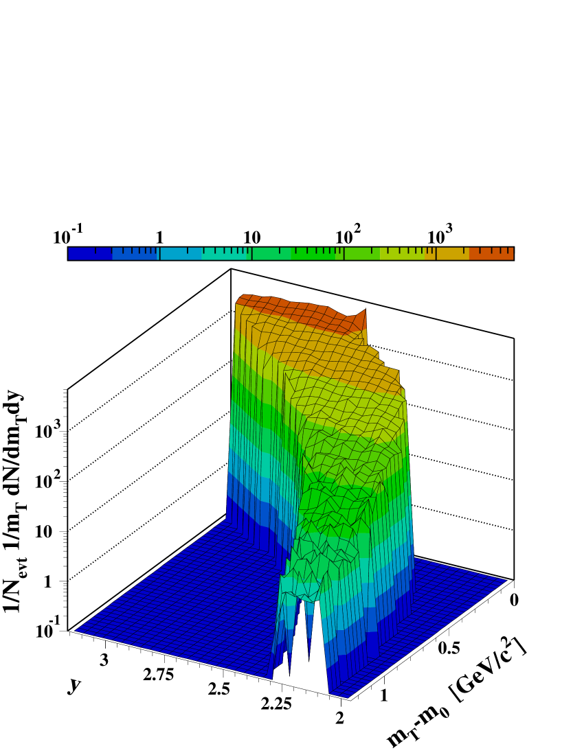
Figure 5: Two-dimensional (fully corrected) single pion spectrum as a function of the two variables $m_{T}$ and $y$.

Figure 6 shows the projection on the $m_{T}$ axis (normalized to a unit rapidity interval using the VENUS profile) of the two-dimensional spectrum of Fig. 5. A fit to the exponential form of eq. 2 over the interval $m_{T}-m_{0}=[0.1,1.2]{{\;{\mathrm{GeV}}/c^{2}}}$ (not shown in Fig. 6) yields $C=5220\pm 80\ (stat.)\ {\!\!\mbox{\tiny$\begin{array}[]{l}+1270\vspace*{-0.7ex}\\ -200\vspace*{0.7ex}\end{array}$ }}(syst.)$, and $T=0.168\pm 0.001\ (stat.)\ {\!\!\mbox{\tiny$\begin{array}[]{l}+0.001\vspace*{-0.7ex}\\ -0.005\vspace*{0.7ex}\end{array}$ }}(syst.){{\;{\mathrm{GeV}}}}$, with a $\chi^{2}$ per degree of freedom of 1.6. This result is in agreement with the NA49 result [13].

At high $p_{T}$, where perturbative QCD becomes applicable, the spectra are expected to attain a power-law behaviour as observed in numerous high energy pp measurements (see for example [14]). The heavy-ion data of this experiment seem to follow that trend even into the lower $p_{T}$ range. Therefore, a parametrization originally inspired by QCD [15] and successfully applied already to pp data [14] and heavy-ion data [16] can be used to fit the spectrum:

$$E\frac{d^{3}\sigma}{dp^{3}}=C\left(\frac{p_{0}}{p_{T}+p_{0}}\right)^{n}$$ (3)

with $C$, $p_{0}$, and $n$ taken as free parameters. A link to the more familiar exponential slope parameter $T$ is obtained from the derivative of this expression according to

$$T_{{\mathrm{power-law}}}=-\frac{f(p_{T})}{\frac{\partial f(p_{T})}{\partial p_{T}}}=\frac{p_{0}}{n}+\frac{p_{T}}{n}\ .$$

Thus, $p_{0}/n$ characterizes the slope of the transverse momentum spectrum in the limit $p_{T}\rightarrow 0$, while $1/n$ characterizes its gradient along $p_{T}$, i.e. the strength of the concave curvature. The extracted parameters are $C=4150\pm 70$, $p_{0}=4.80\pm 1.04{{\;{\mathrm{GeV}}/c}}$ and $n=29.0\pm 5.9$, which gives a slope parameter $T\equiv p_{0}/n=0.166\pm 0.005{{\;{\mathrm{GeV}}}}$. The $\chi^{2}$ per degree of freedom is 1.0. The same fit performed on the $\pi^{0}$ spectrum measured by the WA98 experiment [7, 6, 17, 18] yields $C=5120\pm 140$, $p_{0}=5.08\pm 0.18{{\;{\mathrm{GeV}}/c}}$, $n=29.3\pm 0.8$, and so $T=0.173\pm 0.002{{\;{\mathrm{GeV}}}}$. The acceptance for the $\pi^{0}$ measurement being different, it is interesting to note that fitting only the $p_{T}=[0.3,1.4]{{\;{\mathrm{GeV}}/c}}$ common interval of both spectra yields $T=0.169{{\;{\mathrm{GeV}}}}$ for the $\pi^{-}$ and $T=0.166{{\;{\mathrm{GeV}}}}$ for the $\pi^{0}$, showing that the result is stable with respect to the fit interval and that the spectra agree quite well.

It has also been shown that fluctuation of the parameter in an exponential distribution leads to a final distribution of the power-like form [19]. This behaviour can be interpreted in terms of a suitable application of the nonextensive statistics of Tsallis [20]. This interpretation is convenient to describe particle production at fluctuating $T$, as may occur near the phase transition. These fluctuations would exist in small parts of the hadronic system with respect to the whole system rather than between events. The average $\left<T\right>$ around which the temperature fluctuates is given by $p_{0}/n=0.166$ GeV and the relative variance of $1/T$ is

$$\omega=\frac{\left<(\frac{1}{T})^{2}\right>-\left<\frac{1}{T}\right>^{2}}{\left<\frac{1}{T}\right>^{2}}=\frac{1}{n}=0.034\ ,$$

both for $\pi^{-}$ and $\pi^{0}$. This corresponds to a nonextensivity parameter $q=1+\omega$ of 1.034. This result, interpreted in the spirit of [19], indicates a relative fluctuation $\Delta T/T$ of $18.4\pm 1.9\%$ ($18.4\pm 0.3\%$) for the $\pi^{-}$ ($\pi^{0}$) measurement. However, this analysis neglects the contributions of resonance decays and of flow velocity distributions. Both of these effects increase the curvature of the pion spectrum. Thus the value of $\Delta T/T=18.4\%$ should be considered an upper limit on the temperature fluctuations.

The averaged negative pion yield per unit rapidity in the acceptance window is $1/N_{{\mathrm{evt}}}dN/dy=129\pm 1\ (stat.)\ {\!\!\mbox{\tiny$\begin{array}[]{l}+23\vspace*{-0.7ex}\\ -5\vspace*{0.7ex}\end{array}$ }}(syst.)$.

Figure 6: One-dimensional (fully corrected) $m_{T}$-spectrum for $\pi^{-}$. The errors are statistical. The power-law fit of eq. 3 is superimposed on the data points. The fit interval is $m_{T}-m_{0}=[0.05,1.2]{{\;{\mathrm{GeV}}/c^{2}}}$.

Figure 7: $\pi^{-}$ (black circles) and $K^{-}$ (empty circles) single particle spectra. The error bars are statistical only. Note that for the same transverse mass, the $p_{T}$ is different for pions and kaons. The inset shows the (bin by bin) ratio of the two $p_{T}$ spectra.

Figure 7 shows the same plot as above for kaons. A fit to the exponential form 2 yields $C=1000\pm 120\ (stat.)\ {\!\!\mbox{\tiny$\begin{array}[]{l}+260\vspace*{-0.7ex}\\ -1\vspace*{0.7ex}\end{array}$ }}(syst.)$, and $T=0.181\pm 0.005\ (stat.)\ {\!\!\mbox{\tiny$\begin{array}[]{l}+0.001\vspace*{-0.7ex}\\ -0.009\vspace*{0.7ex}\end{array}$ }}(syst.){{\;{\mathrm{GeV}}}}$. So the inverse slope $T$ for kaons and pions are comparable. It should be noted that the rapidity acceptance is quite different for the two particle species, the $\pi^{-}$ acceptance being much closer to mid-rapidity. An estimate of the effect induced by this difference in acceptance can be made using the term $\cosh(\Delta y)$ given below eq. 1. The inverse slope for $K^{-}$ would become of the order of $0.230{{\;{\mathrm{GeV}}}}$. The $K^{-}/\pi^{-}$ ratio at a common rapidity of 2.3 is $11.4\pm 0.4\ (stat.)\ {\!\!\mbox{\tiny$\begin{array}[]{l}+0.6\vspace*{-0.7ex}\\ -2.7\vspace*{0.7ex}\end{array}$ }}(syst.)\%$, which is in agreement with the NA49 result [13].

3.3 Hydrodynamical Source Expansion Model

The single pion spectrum has been fitted in the interval $0.05<m_{T}-m_{0}<1.2{{\;{\mathrm{GeV}}/c^{2}}}$ with the Wiedemann-Heinz (W.-H.) model [21, 22, 23, 24, 25, 26]. It relies on the following idea: the main characteristics of the particle phase-space distribution at freeze-out can be quantified by its widths in the spatial and temporal directions, a collective dynamical component (parameterized by a flow field) which determines the strength of the position-momentum correlations in the source, and a second, random dynamical component in momentum space (parameterized by a temperature). The model emission function contains seven parameters, but the shape of the single particle transverse mass spectrum is fully determined by the temperature $T$ and the transverse flow rapidity profile $\eta_{T}(r)=\eta_{f}\frac{r}{R}$ which is assumed to depend linearly on the transverse coordinate $r$, where $\eta_{f}$ is the transverse flow rapidity strength, and $R$ the Gaussian transverse spatial width. The mean transverse flow velocity $\left<\beta_{T}\right>$ can be easily calculated as the mean value of $\tanh(\eta_{T}(r))$ over the transverse source profile. The results will be given as a function of $\left<\beta_{T}\right>$ rather than $\eta_{f}$, since its physical interpretation is more straightforward.

The three parameters that are allowed to vary freely during the fitting procedure are $T$, $\eta_{f}$, and an overall normalization factor. The result of the fit is $T=0.084\pm 0.003{{\;{\mathrm{GeV}}}}$ and $\left<\beta_{T}\right>=0.50\pm 0.02$, the $\chi^{2}/d.o.f.$ being 1.1. The resulting curve is not shown in Fig. 6 as it is hardly distinguishable from the power-law fit. The temperature and flow parameters are strongly correlated, so it is more interesting to consider a $\chi^{2}$ contour plot of the fit to the measured single particle spectrum as a function of those two parameters. Figure 8 shows the result assuming a Gaussian transverse spatial profile, and Fig. 9 assuming a box profile of the same rms width as the Gaussian one. Only direct pions are considered in the model. Furthermore, only statistical errors are taken into account during the fit. The curves displayed represent different confidence levels for the $(T,\left<\beta_{T}\right>)$ values.

Figure 8: $\chi^{2}$ contour plot of the hydrodynamical model fit to the measured $\pi^{-}$ single particle spectrum of Fig. 6. A Gaussian profile is assumed for the transverse spatial profile of the source. The curves displayed represent successively (starting with the innermost one) contours at 50% CL, 90% CL, 99% CL (dashed line), 99.9% CL, and the last curve indicates a highly excluded region. The black square represents the best parameter values.

Figure 9: Same plot as in Fig. 8, but assuming a box profile for the transverse spatial profile of the source.

The dependence of the $\chi^{2}/d.o.f.$ on the shape of the source is very small, the best $\chi^{2}/d.o.f.$ being slightly larger for the box profile (1.5). While the best fit temperature appears to be independent of the shape of the source, the best fit flow velocity is considerably smaller ($\left<\beta_{T}\right>=0.29$) for the box profile. Inclusion of the resonance decay contribution in the model calculation would be expected to reduce the extracted flow velocity parameters and increase the temperature parameters. The precise effects do however depend on details of the models used.

4 Two-pion correlations

Bose-Einstein interferometry is most commonly used to study pairs of identical particles. The correlation function $C_{2}$ is defined, up to a proportionality factor $\cal N$, as the ratio of a two-particle spectrum ${\cal P}_{2}$ over the product of two single particle spectra ${\cal P}_{1}$:

$$C_{2}({\vec{p}}_{1},{\vec{p}}_{2})={\cal N}\;\frac{{\cal P}_{2}({\vec{p}}_{1},{\vec{p}}_{2})}{{\cal P}_{1}({\vec{p}}_{1})\cdot{\cal P}_{1}({\vec{p}}_{2})}$$

with

$${\cal P}_{1}({\vec{p}})=E\;\frac{dN}{d{p}^{3}}$$

and

$${\cal P}_{2}({\vec{p}}_{1},{\vec{p}}_{2})=E_{1}\;E_{2}\;\frac{dN}{dp^{3}_{1}\;dp^{3}_{2}}$$

where $E_{i}$ and $\vec{p}_{i}$ are the energy and momentum of particle $i$, respectively.

Experimentally, the product of one-particle distributions in the denominator is commonly obtained by a mixed event technique whereas the two-particle distribution in the numerator is constructed from all pair combinations of identical particles found in each event. $C_{2}$ is then normalized to unity far away from the interference region.

A fully chaotic source can be seen as a superposition of uncorrelated elementary sources, and one- and two-particle distributions may be expressed through the Wigner function of the source $S(x,k_{12})$ [1]. The correlation function is then written

$$C_{2}({\vec{p}}_{1},{\vec{p}}_{2})=1\;+\;\lambda\;\frac{|\int\!\>d^{4}x\;S(x,k_{12})\;\exp[iq_{12}x]|^{2}}{|\int\!\>d^{4}x\;S(x,k_{12})|^{2}}$$

with $q_{12}=p_{1}-p_{2}$, the 4–momentum difference of the two particles, $k_{12}=(p_{1}+p_{2})/2$ and $x=(x_{1}+x_{2})/2$, the mean space-time coordinate of the pair emission point. The chaoticity parameter $\lambda$ is inserted to take into account the possibility that the source may not be fully chaotic and also that any wrongly reconstructed tracks, or tracks originating from decays of long-lived resonances, will dilute the Bose-Einstein correlations in the data.

A one-dimensional interferometry analysis is commonly made as a function of $Q_{inv}\equiv\sqrt{-q_{12}^{2}}$, whereas a multidimensional analysis uses a set of $Q$ variables which are defined as various projections of $q_{12}$.

4.1 Data analysis and results

Two independent analyses were performed with the complete data set recorded in the negative tracking arm [11, 27] totalling 13.7$\times 10^{6}$ pairs of identified $\pi^{-}$. These data were corrected for resolution and Coulomb effects in an iterative way [28]. The Gamow correction was not used as it overcorrects the data in the $Q_{inv}$ range of 0.1 to 0.3 GeV/$c$. Because the finite resolution in the measurement of the $Q$ variables leads to an underestimate of the radii and $\lambda$ parameters, a correction has to be implemented in the fitting procedure. This is done by a convolution method, replacing the $C_{2}(\vec{Q})$ formula expressing the two-particle correlation function used to fit the data by

$$C_{2}^{rc}(\vec{Q})=\int\!\!\int\!\!\int r(\vec{Q},\vec{Q^{\prime}})\>C_{2}(\vec{Q^{\prime}})\>d\vec{Q^{\prime}}$$

where $r(\vec{Q},\vec{Q^{\prime}})$ is the resolution function which is chosen to be Gaussian:

$$r(\vec{Q},\vec{Q^{\prime}})=1/(2\pi)^{3/2}\>1/|V|^{1/2}\>$$

$$\hskip 42.67912pt\times\exp[-1/2\>(\vec{Q}-\vec{Q^{\prime}})^{T}\>V^{-1}\>(\vec{Q}-\vec{Q^{\prime}})]$$

The diagonal elements of the covariance matrix $V$ are set equal to the square of the various $Q$-resolutions, which are estimated by a full simulation of the experimental setup as a function of the $k_{T}=|\vec{p}_{T1}+\vec{p}_{T2}|/2$ of the pairs. The non-diagonal elements of $V$ are neglected, as the resolution correction has a very small effect compared to the Coulomb correction. Figure  10 shows $C_{2}$, the measured $\pi^{-}$$\pi^{-}$ correlation function, plotted as a function of $Q_{inv}$ before and after the resolution and Coulomb corrections. In the plot, the correction for resolution is obtained by multiplying each data point by $C_{2}^{rc}(Q_{inv})/C_{2}(Q_{inv})$. $C_{2}$ is clearly exponential [29]. The solid curve is a fit of the form 1+$\lambda_{e}$exp[-2$Q_{inv}R_{inv}]$ which gives $R_{inv}=7.33\pm 0.08$ fm and $\lambda_{e}=0.788\pm 0.009$ for $\left<k_{T}\right>=0.116$ GeV/$c$. This exponential behaviour appears not to hold in the 3-d analysis, where the projected slices are better represented by Gaussians.

Figure 10: The measured two-pion correlation function $C_{2}$ (full symbols), corrected for resolution and Coulomb effects, as a function of $Q_{inv}$. The full line is a fit to an exponential form whereas the dashed curve is a fit to a Gaussian form. The empty symbols show the data before corrections.

Figure 11: The $k_{T}$ dependence of the Pratt-Bertsch parameters. The points are plotted at the average $k_{T}$ of the bin and the horizontal bars indicate the bin width. The open symbols in the figure at bottom right show the $\lambda$ parameter after correction for background from misidentified pions, as explained in section  5.

The 3-d analysis of Bose-Einstein correlations has been done using two different parameterizations in the Longitudinally CoMoving System (LCMS): the standard Pratt-Bertsch fit (PB) in the 3-dimensional space of momentum differences $Q_{TS}$ (perpendicular to the beam axis and to the transverse momentum of the pair), $Q_{TO}$ (perpendicular to the beam axis and parallel to the transverse momentum of the pair), and $Q_{L}$ (parallel to the beam axis) [30], including a cross term $R^{2}_{out-long}$ as predicted [31]

$$C_{2}=1+\lambda\exp[-Q_{TS}^{2}R_{TS}^{2}-Q_{TO}^{2}R_{TO}^{2}-Q_{L}^{2}R_{L}^{2}$$

$$\hskip 110.96556pt-2Q_{TO}Q_{L}R^{2}_{out-long}]$$

and the Yano-Koonin-Podgoretskiĭ fit (YKP) [21] in the $Q_{0}$ (energy difference of the pair), $Q_{T}$,$Q_{L}$ space

$$C_{2}=1+\lambda\exp[-Q^{2}_{T}R^{2}_{T}+(Q^{2}_{0}-Q^{2}_{L})R^{2}_{4}-(Q{\cdot}U)^{2}(R^{2}_{0}+R^{2}_{4})]$$

where $U=\gamma(1,0,0,v_{L})$, $\gamma=1/\sqrt{1-v_{L}^{2}}$ with $v_{L}$ in units of $c=1$. In the YKP parameterization the different radii are invariant under a longitudinal Lorentz boost, and the speed parameter $v_{L}$ connects the local rest frame to the measurement frame (the LCMS in our case). The results as a function of the $k_{T}$ of the pairs are shown in Figs. 11 and  12 and summarized in Table 1. The $\lambda$ parameters of the YKP fit (not shown in Table 1) are found compatible with the $\lambda$ parameters of the PB fit.

Figure 12: Comparison between the PB and YKP fits in the LCMS. The cross term $R^{2}_{out-long}$ from the PB fit and $v_{L}$ from the YKP fit both show a deviation from zero at large $k_{T}$ when estimated in the LCMS. The $R_{TS}$ and $R_{L}$ parameters from the PB fit are in good agreement with respectively $R_{T}$ and $R_{4}$ from the YKP fit.

The systematic errors, not included in Figs. 11 and  12, and Table 1, are estimated by varying the different analysis cuts, including the cuts used to identify the pion with the time of flight system. The systematic error on the Coulomb correction due to the error on the determination of the radius parameters is also taken into account. All these variations are added in quadrature. The total relative systematic errors on the radii $\Delta{R}/R$ amount to 0.8% for $R_{inv}$, 1.4% for $R_{TS}$, 3.5% for $R_{TO}$, 9.1% for $R_{L}$, 0.8% for $R_{T}$, and 9.7% for $R_{4}$. Systematic errors on $R^{2}_{out-long}$ and $v_{L}$ are asymmetric and reach respectively $\begin{array}[]{l}+2.2\vspace*{-0.7ex}\\ -1.7\vspace*{0.7ex}\end{array}$ fm² and $\begin{array}[]{l}+0.13\vspace*{-0.7ex}\\ -0.08\vspace*{0.7ex}\end{array}$ .

The $R_{TS}$ and $R_{L}$ parameters from the PB fit are in good agreement respectively with $R_{T}$ and $R_{4}$ from the YKP fit. The cross term $R^{2}_{out-long}$ from the PB fit and $v_{L}$ from the YKP fit deviate from zero. In a source undergoing a boost invariant expansion the local rest frame coincides with the LCMS. Both the cross term and $v_{L}$ expressed in the LCMS are then expected to vanish [21]. As this is not quite the case, it suggests that the source seen within the acceptance does not have a strictly boost invariant expansion. The strong decrease of the longitudinal radius $R_{L}$ or $R_{4}$ with $k_{T}$ compared to the transverse radii $R_{T}$, $R_{TS}$, $R_{TO}$ shows a longitudinal expansion which is larger than the transverse one. Finally, the $R_{0}$ parameter (not shown in the figures), which corresponds to the duration of emission of particles from the source, is compatible with zero for all $k_{T}$ bins, excluding a long-lived intermediate phase. These results agree with the previously published WA98 results obtained using roughly half of the present data sample [29]. The WA98 analysis is compatible with the NA49 results obtained in a slightly different rapidity range ($\left<y\right>=3.2$) with unidentified negative particles [32].

4.2 Comparison with a hydrodynamical model based simulation

The W.-H. model can be used to generate correlation functions which can be compared to the data. For that purpose, all necessary integrations are performed numerically [25] to get the value of $C_{2}$ in the PB parameterization for given values of $Q_{TS}$, $Q_{TO}$, $Q_{L}$, $k_{T}$, and the rapidity $Y=(y_{1}+y_{2})/2$ of a pair. To simulate properly the acceptance of the negative tracking arm, the mean values of $k_{T}$ and $Y$ for each $(Q_{TS},Q_{TO},Q_{L})$ bin are calculated using real data, and then for each bin the mean values $(\left<Q_{TS}\right>,\left<Q_{TO}\right>,\left<Q_{L}\right>,\left<k_{T}\right>,\left<Y\right>)$ are used as input for the hydrodynamical calculation. This procedure is repeated for all five $k_{T}$ intervals used in the data analysis. The correlation functions are generated neglecting contribution from resonances, using $T=85$ MeV, $\eta_{f}=0.5$ (values extracted from the single particle spectra analysis), $R=8$ fm, $\tau_{0}=11$ fm/$c$, $\Delta\tau=2$ fm/$c$ and $\Delta\eta=1.3$ (see [25] for definitions of the parameters). Figure 13 shows the Bose-Einstein radii extracted from fitting the simulated correlation functions with the PB formula. The error bars used to perform these fits are taken to be the same as the ones calculated for the real data in each $(Q_{TS},Q_{TO},Q_{L})$ bin. The measured results are shown on the same plot, and the agreement is found to be good. The shift in the the cross term $R^{2}_{out-long}$ between data and simulation is compatible with the systematic uncertainty.

Figure 13: Comparison between simulation and data as a function of $k_{T}$. The open symbols are the result of the fit of the PB formula to the correlation functions produced by the hydrodynamical model, whereas the full symbols are the result of the fit to the data.

5 Average pion phase-space density at freeze-out

As the $m_{T}$ spectrum gives the momentum-space density at freeze-out and as the Bose-Einstein correlation radii provide information on the covariant volume for particles of momentum $\vec{p}$, it is possible, by combining these results, to extract the average phase-space density $\left<f\right>(p_{T},y)$ at freeze-out [33, 34]:

$$\left<f\right>=\frac{\sqrt{\lambda}}{(\frac{E_{\pi}}{\pi^{3/2}})R_{TS}\sqrt{R_{TO}^{2}R_{L}^{2}-R^{4}_{out-long}}}{\ }\frac{dn}{{dy}{\ }{p_{T}}{\ }{dp_{T}}{\ }{d\phi}}$$

with $E_{\pi}=\sqrt{m_{\pi}^{2}+p^{2}}=m_{T}\cosh{y}$. The radii and $\lambda$ are functions of $p_{T}$ and $y$. The factor $\lambda$, which comes from the two-pion correlation analysis, corrects for contributions of pions originating from long-lived resonances decaying close to the primary vertex. A difficulty of this method is to include only the contribution of the real pions in the determination of $\lambda$, excluding backgrounds from misidentified particles. This is achieved by applying to $\lambda$, separately for each $k_{T}$ bin, a correction factor obtained from a full simulation of the experimental setup, taking into account geometrical acceptance, backgrounds and efficiency of the chamber-camera-time of flight system. The effects can be seen in Fig. 11, bottom right, where $\lambda$ with and without correction is displayed.

Figure 14: Average pion phase-space density as a function of $p_{T}$ compared to different models (see text).

Figure 14 and Table 2 show the results on the average phase-space density for $\pi^{-}$ as a function of $p_{T}$. The error bars reflect the statistical errors only. The systematic uncertainties are dominated by the uncertainty of the correction on the $\lambda$ parameter, which is estimated to be 20%, and by the systematic error on $R_{L}$, giving a total of 13.7% systematic error on $\left<f\right>$. Within errors, all nuclear collision measurements at the SPS are found to be indistinguishable [35], and our result at mid-rapidity agrees well with these previous measurements. The dashed lines indicate Bose-Einstein density distributions $\left<f\right>=[\exp(E_{\pi}/T)-1]^{-1}$ of static sources of pions ($E_{\pi}\approx m_{T}$) for three choices of the freeze-out temperature $T$: 80 MeV, 100 MeV, and 120 MeV, from the lower to the higher curve. The results are in rough agreement with the 100 MeV distribution at low $p_{T}$, but show a clear deviation from a Bose-Einstein distribution at high $p_{T}$. As pointed out in [36], this deviation is mainly due to the strong longitudinal expansion of the fireball which reduces the spatially averaged phase-space density and, to a lesser extent, due to the radial collective flow, which adds extra transverse momentum to the particles compared to particles emitted by a static source. Consequently, even in the absence of transverse flow, $\left<f\right>$ will be reduced compared to a Bose-Einstein density distribution. This effect may necessitate a positive pion chemical potential in order to match the experimental observation. Such a positive potential can be related to the presence of pions from short-lived resonance decays. The Tomás̆ik-Heinz (T.-H.) model [36] used to fit the data assumes a thermalized fireball with a longitudinally boost-invariant expansion and a transverse flow rapidity profile which depends linearly on the transverse coordinate. This model includes a pion chemical potential and has three free parameters, the freeze-out temperature $T$, the strength of the transverse flow rapidity profile $\eta_{t}$, and $\mu_{0}$, the chemical potential value in the center of the fireball. In Fig. 14, the full line is a fit of the T.-H. model with a box transverse density profile, whereas the point-dashed line is a fit of the same model with a Gaussian transverse profile. Both fits agree well with the data with a $\chi^{2}/d.o.f.$ of 0.78 and 0.93 for respectively the box and the Gaussian profiles, giving $T=87\!\!\mbox{\tiny$\begin{array}[]{l}+52\vspace*{-0.7ex}\\ -27\vspace*{0.7ex}\end{array}$ }$ MeV, $\eta_{t}=0.49\!\!\mbox{\tiny$\begin{array}[]{l}+0.07\vspace*{-0.7ex}\\ -0.22\vspace*{0.7ex}\end{array}$ }$ and $\mu_{0}=57\!\!\mbox{\tiny$\begin{array}[]{l}+29\vspace*{-0.7ex}\\ -125\vspace*{0.7ex}\end{array}$ }$ MeV for the box profile. This $\eta_{t}$ result corresponds to a mean transverse flow velocity $\left<\beta_{T}\right>=0.42\!\!\mbox{\tiny$\begin{array}[]{l}+0.05\vspace*{-0.7ex}\\ -0.18\vspace*{0.7ex}\end{array}$ }$.

Figure 15: $\chi^{2}$ contour plot for the T.-H. model with a box profile. Starting from the centre, the curves represent contours at 39%, 70% and 99% confidence level for $T$ and $\eta_{t}$. The black square is the best fit ($\mu_{0}=57$ MeV). The full circle is the result with $\mu_{0}$ excluded from the fit and set to zero.

Due to the lack of experimental points at large $p_{T}$, the T.-H. model with the Gaussian profile provides very loose estimates of these parameters, which are nevertheless compatible with those from the box profile. Figure 15 shows the $\chi^{2}$ contour plot for the T.-H. model with the box profile for $T$ and $\eta_{t}$. The curves represent (starting from the centre) contours at 39%, 70% and 99% confidence level. The best fit is obtained for a pion chemical potential $\mu_{0}=57$ MeV (black square) but a solution with $\mu_{0}=0$ MeV is also possible (full circle). On the other hand, a large pion chemical potential at freeze-out, close to the Bose condensation limit of $\mu_{0}=m_{\pi}$, as could be speculated given the rather low mass of the pion, seems to be excluded in view of the error bar on $\mu_{0}$. The results of the fit of the W.-H. model on the single $\pi^{-}$ spectrum can be compared to the fit of the T.-H. model on the phase-space distribution. The agreement is good for $T$, and satisfactory for $\left<\beta_{T}\right>$ when taking into account the systematic error. It should be noted that the constraint provided by the fit of the T.-H. model is weak compared to the one given by the W.-H. model because of the relatively small amount of experimental points in the phase-space distribution. Moreover the T.-H. model uses a pion chemical potential whereas the W.-H. model doesn’t. Finally, as $\left<f\right>$ is the pion occupation per 6-d position$\otimes$momentum cell, the obtained values do not provide striking evidence for the presence of an excess of pions or for the presence of large disoriented chiral condensates. This chiral condensate phenomena has been investigated by other means within WA98 [37, 38].

6 Three-pion correlations

In the hypothesis of a fully chaotic source of identical particles, the two-pion correlation function can be written $C_{2}=1+|F_{12}|^{2}$ where $|F_{12}|^{2}$ is the Fourier transform squared of the space-time source function. The three-pion correlation function is then $C_{3}=1+|F_{12}|^{2}+|F_{23}|^{2}+|F_{31}|^{2}+2\cdot\mbox{Re}\{F_{12}\cdot F_{23}\cdot F_{31}\}$. The terms $|F_{ij}|^{2}$, which express the contribution of the three combinations of the two-pion correlations contained in the triplet (123), provide the largest contribution to $C_{3}$. The last term only represents the genuine three-body correlation. It can be written $2\cdot|F_{12}|\cdot|F_{23}|\cdot|F_{31}|\cdot W$, where $F_{ij}$ is defined as $|F_{ij}|\exp[i\phi_{ij}]$ and $W\equiv\cos(\phi_{12}+\phi_{23}+\phi_{31})$. The simultaneous measurement of $C_{2}$ and $C_{3}$ provides information on $W$, the cosine of the sum of the three phases of the Fourier transforms. In contrast, the measurement of $C_{2}$ alone gives access only to the radii of the source and not to the phases. If the emission source is fully chaotic, $W$ measures the asymmetry of the source. In the presence of not fully chaotic sources, which is likely to be the case, $W$, the strength of the true three-body correlation, is basically sensitive to the coherence. So, in the framework of the partially coherent model [39], $W$ gives information on the degree of chaoticity of the emission source in a manner which is insensitive to backgrounds such as the contributions from resonances. The complete data set recorded with the negative tracking arm yielded a total of 13.1$\times 10^{6}$ triplets of $\pi^{-}$.

Figure 16: The three-pion correlation function $C_{3}$ as a function of $Q_{3}$. The full line is a fit to a double exponential form (see text). The dotted and the dashed lines are fits to respectively a single exponential and a Gaussian form.

After correction for resolution and Coulomb effects , a strong $C_{3}$ signal is observed (Fig. 16) as a function of $Q_{3}\equiv\sqrt{Q_{12}^{2}+Q_{23}^{2}+Q_{31}^{2}}$ with $Q_{ij}\equiv\sqrt{-(p_{i}-p_{j})^{2}}$, which can be fitted by a double exponential function

$$C_{3}=1+\lambda_{1}\exp[-2Q_{3}R_{1}]+\lambda_{2}\exp[-2Q_{3}R_{2}]$$

with fitted parameters $R_{1}=5.08\pm 0.26$ fm, $\lambda_{1}=3.12\pm 0.27$, $R_{2}=1.66\pm 0.08$ fm, $\lambda_{2}=0.341\pm 0.046$ and $\chi^{2}/d.o.f.=1.10$. Such non-Gaussian behaviour was in fact predicted by a final-state rescattering model [40]. After the measurement of $C_{2}$ and $C_{3}$, the data are analysed again and the experimental value of $W$ is calculated using

$$W=\frac{\{C_{3}(Q_{3})-1\}-\{C_{2}(Q_{12})-1\}-\{C_{2}(Q_{23})-1\}-\{C_{2}(Q_{31})-1\}}{2\cdot\sqrt{\{C_{2}(Q_{12})-1\}\{C_{2}(Q_{23})-1\}\{C_{2}(Q_{31})-1\}}}$$

individually for each triplet found, characterized by $Q_{3}$ and by the values $Q_{12}$, $Q_{23}$, and $Q_{31}$ corresponding to the three pair combinations contained in the triplet.

Figure 17: The factor $W$ as a function of $Q_{3}$. The error bars include statistical and systematic errors. The statistical errors alone are contained within the size of the symbols.

As described earlier, the estimate of systematic errors is done by varying the different analysis cuts, both in the two- and three-pion correlation analysis. The effects on $W$ of the statistical errors in the measurement of $C_{2}$ and $C_{3}$ are treated as systematic errors by changing $C_{2}$ ($C_{3}$) by $\pm\sigma_{C_{2}}$ ($\pm\sigma_{C_{3}}$). This last source of error dominates the other ones. All these variations are then added in quadrature.

Figure 17 and Table 3 show $W$ as a function of $Q_{3}$ for $Q_{3}\leq 60$ MeV/$c$, beyond which the $W$ significance is too low. The error bars include statistical and systematic errors. The statistical errors (not shown separately in Fig. 17) are by comparison negligible. In view of the errors, no significant $Q_{3}$ dependence is observed. The genuine three-pion correlation is found to be substantial with a weighted mean over the five bins $\left<W\right>=0.735\pm 0.004(stat.)\pm 0.146(syst.)$.

This result is in agreement with the previously published WA98 result obtained using about half of the present data sample [41], where a more detailed description of the three-pion analysis method can also be found. More recently, the NA44 experiment [42] obtained with lower statistics a factor $\left<W\right>$ which agrees with our results.

7 Conclusions

We have studied $m_{T}$ distributions for identified $\pi^{-}$ and $K^{-}$ produced in central Pb+Pb collisions at 158$A$ GeV. The W.-H. hydrodynamical model has been fitted to the pion spectrum. The resulting fitted parameters favor a combination of a relatively low temperature $T$ $\sim$85 MeV and an average transverse flow velocity $\left<\beta_{T}\right>$ $\sim$0.50. The shape of the $\pi^{-}$ $m_{T}$ distribution is in good agreement with the $\pi^{0}$ $m_{T}$ distribution measured in the same experiment.

Bose-Einstein interferometry of $\pi^{-}$ pairs gives fitted radii of typically 7 fm. This has to be compared to the equivalent rms radius of the initial Pb ion of 3.2 fm, indicating an expanded emission volume at freeze-out.

The analysis of two-pion correlations has been performed as a function of $k_{T}$ using two different parameterizations in the LCMS. The results are consistent between the standard 3-dimensional Pratt-Bertsch fit and the Yano-Koonin-Podgoretskiĭ fit.

A clear dependence of all radius parameters on $k_{T}$ is observed, with a stronger dependence for the longitudinal radii, indicating a larger longitudinal than transverse expansion. Both the cross term $R^{2}_{out-long}$ from the PB fit and $v_{L}$ from the YKP fit deviate from zero, which suggests that the source seen within the acceptance does not undergo a strictly boost invariant expansion. Moreover the short duration of emission disfavours any long-lived intermediate phase.

A comparison of the data with a hydrodynamical simulation based on the Wiedemann-Heinz model, and taking into account acceptance and resolution effects has been made for the radii parameters as a function of $k_{T}$. The agreement is found to be very good.

The average pion phase-space density at freeze-out has been calculated from measured quantities as a function of $p_{T}$. The results indicate a clear deviation from a Bose-Einstein distribution at high $p_{T}$, but are very well fitted by the Tomás̆ik-Heinz model. The pion chemical potential, which is included in the model, is found to be compatible with zero, while a large pion chemical potential close to the condensation limit of $m_{\pi}$, seems to be excluded.

Finally, we have studied the $\pi^{-}\pi^{-}\pi^{-}$ interference and found a substantial contribution of genuine three-pion correlations in central collisions. For $Q_{3}\leq$60 MeV/$c$ a weighted mean of the strength of the genuine three-pion correlations $\left<W\right>=0.735\pm 0.004(stat.)\pm 0.146(syst.)$ was extracted. This is somewhat smaller than what is expected for a fully chaotic and symmetric source.

Acknowledgements
   We would like to thank the CERN-SPS accelerator crew for providing an excellent Pb beam. This work was supported jointly by the German BMBF and DFG, the U.S. DOE, the Swedish NFR, the Dutch Stichting FOM, the Swiss National Fund, the Humboldt Foundation, the Stiftung für deutsch-polnische Zusammenarbeit, the Department of Atomic Energy, the Department of Science and Technology and the University Grants Commission of the Government of India, the Indo-FRG Exchange Programme, the PPE division of CERN, the INTAS under contract INTAS-97-0158, the Polish KBN under the grant 2P03B16815, the Grant-in-Aid for Scientific Research (Specially Promoted Research & International Scientific Research) of the Ministry of Education, Science, Sports and Culture, JSPS Research Fellowships for Young Scientists, the University of Tsukuba Special Research Projects, and ORISE. ORNL is managed by UT-Battelle, LLC, for the U.S. Department of Energy under contract DE-AC05-00OR22725.

Table 1: 3-dimensional analysis as a function of $k_{T}$ for the PB and the YKP fits. $\lambda$ after correction for backgrounds from misidentified pions is also shown.

$\left<k_{T}\right>$	0.02 GeV/$c$		0.07 GeV/$c$		0.125 GeV/$c$		0.175 GeV/$c$		0.285 GeV/$c$
$R_{TS}$	6.48$\pm$	0.18 fm	6.67$\pm$	0.15 fm	5.55$\pm$	0.24 fm	5.13$\pm$	0.32 fm	4.81$\pm$	0.29 fm
$R_{TO}$	6.95$\pm$	0.20 fm	6.62$\pm$	0.16 fm	6.70$\pm$	0.29 fm	6.29$\pm$	0.43 fm	6.07$\pm$	0.50 fm
$R_{L}$	8.69$\pm$	0.26 fm	7.54$\pm$	0.19 fm	5.95$\pm$	0.27 fm	5.45$\pm$	0.37 fm	5.15$\pm$	0.34 fm
$R^{2}_{out-long}$	1.51$\pm$	2.11 fm2	0.55$\pm$	1.45 fm2	-0.52$\pm$	1.96 fm2	-3.01$\pm$	2.31 fm2	-4.51$\pm$	1.94 fm2
$\lambda$	0.334$\pm$	0.012	0.362$\pm$	0.010	0.337$\pm$	0.018	0.324$\pm$	0.026	0.391$\pm$	0.036
$\lambda_{cor}$	0.646$\pm$	0.023	0.634$\pm$	0.018	0.557$\pm$	0.030	0.511$\pm$	0.041	0.596$\pm$	0.055
$R_{T}$	6.66$\pm$	0.14 fm	6.54$\pm$	0.13 fm	5.99$\pm$	0.19 fm	5.78$\pm$	0.29 fm	5.17$\pm$	0.26 fm
$R_{4}$	8.68$\pm$	0.26 fm	7.52$\pm$	0.19 fm	5.97$\pm$	0.28 fm	5.49$\pm$	0.39 fm	4.94$\pm$	0.35 fm
$v_{L}$	0.02$\pm$	0.08 fm	-0.04$\pm$	0.06 fm	0.08$\pm$	0.08 fm	0.14$\pm$	0.10 fm	0.20$\pm$	0.09 fm

Table 2: Average $\pi^{-}$ phase-space density $\left<f\right>$ at freeze-out as a function of $p_{T}$.

$\left<p_{T}\right>$	0.02 GeV/$c$		0.07 GeV/$c$		0.125 GeV/$c$		0.175 GeV/$c$		0.285 GeV/$c$
$\left<f\right>$	0.319$\pm$	0.018	0.272$\pm$	0.012	0.237$\pm$	0.019	0.182$\pm$	0.022	0.088$\pm$	0.012

Table 3: Weighted mean of the strength of the genuine three-pion correlations $\left<W\right>$ as a function of $Q_{3}$.

$Q_{3}$	0.01 - 0.02 GeV/$c$		0.02 - 0.03 GeV/$c$		0.03 - 0.04 GeV/$c$		0.04 - 0.05 GeV/$c$		0.05 - 0.06 GeV/$c$
$\left<W\right>$	0.830	$+0.201$ $-0.175$	0.780	$+0.156$ $-0.143$	0.736	$+0.145$ $-0.138$	0.654	$+0.177$ $-0.193$	0.557	$+0.258$ $-0.293$

References

-
[1]
W. Zajc et al., Phys. Rev. C29, 2173 (1984)
and references therein.
U.A. Wiedemann and U. Heinz, Phys. Rep. 319, 145 (1999) and references therein. - [2] I.V. Andreev, M. Plümer, and R.M. Weiner, Int. J. Mod. Phys. A8, 4577 (1993).
- [3] B. Lörstad, Int. J. Mod. Phys. A4, 2861 (1989) and references therein.
- [4] H. Heiselberg and A.P. Vischer, Phys. Rev. C55, 874 (1997).
- [5] WA98 collaboration, Proposal for a large acceptance hadron and photon spectrometer, 1991, Preprint CERN/SPSLC 91-17, SPSLC/P260.
- [6] M.M. Aggarwal et al., Eur. Phys. J. C23, 225 (2002).
- [7] M.M. Aggarwal et al., nucl-ex/0006007 (2000).
-
[8]
J.M. Rubio et al., Nucl. Instr. and Meth. A367,
358 (1995).
A.L.S. Angelis et al., Nucl. Phys. A566, 605c (1994).
M. Iżycki et al., Nucl. Instr. and Meth. A310, 98 (1991). - [9] E. Schnedermann et al., Phys. Rev. C48, 2462 (1993).
- [10] U. Heinz, in : , edited by H.H. Gutbrod, J. Letessier and J. Rafelski (Plenum Press, ADDRESS, 1995), Vol. 346 of NATO ASI Series B, p. 413.
- [11] S. Vörös, Ph. D. thesis, University of Geneva (2001).
- [12] K. Werner, Phys. Rep. 232, 87 (1993).
- [13] S.V. Afanasiev et al., nucl-ex/0205002.
- [14] G. Bocquet et al., Phys. Lett. B366, 434 (1996).
- [15] R. Hagedorn, Nuovo Cim. 6, 1 (1983), also CERN-TH 3684 (1983).
- [16] R. Albrecht et al., Eur. Phys. J. C5, 255 (1998).
- [17] M.M. Aggarwal et al., Phys. Rev. Lett. 81, 4087 (1998); and Erratum ibid. 84, 578 (2000).
- [18] M.M. Aggarwal et al., Phys. Rev. Lett. 83, 926 (1999).
- [19] G. Wilk and Z. Włodarczyk, Physica A305, 227 (2002) and references therein.
- [20] C. Tsallis, J. Stat. Phys. 52, 479 (1988).
- [21] S. Chapman et al., Phys. Rev. C52, 2694 (1995) and references therein.
- [22] S. Chapman et al., Heavy Ion Physics 1, 1 (1995).
- [23] U. Heinz et al., Phys. Lett. B382, 181 (1996).
- [24] U.A. Wiedemann, P. Scotto and U. Heinz, Phys. Rev. C53, 918 (1996).
- [25] U.A. Wiedemann and U. Heinz, Phys. Rev. C56, 3265 (1997); these calculations were made with a Fortran program supplied by U.A. Wiedemann.
- [26] U.A. Wiedemann and U. Heinz, Phys. Rep. 319, 145 (1999).
- [27] L. Rosselet et al., Nucl. Phys. A698, 647c (2002).
- [28] S.Pratt et al., Phys. Rev. C42, 2646 (1990); these calculations were made with a Fortran program supplied by S. Pratt.
- [29] M.M. Aggarwal et al., Eur. Phys. J. C16, 445 (2000).
-
[30]
S. Pratt, Phys. Rev. D33, 1314 (1986).
G. Bertsch and G.E. Brown, Phys. Rev. C40, 1830 (1989). - [31] S. Chapman et al., Phys. Rev. Lett. 74, 4400 (1995).
- [32] R. Ganz et al., Nucl. Phys. A661, 448c (1999).
- [33] G.F. Bertsch, Phys. Rev. Lett. 72, 2349 (1994); and Erratum ibid. 77, 789 (1996).
- [34] J. Barrette et al., Phys. Rev. Lett. 78, 2916 (1997).
- [35] D. Ferenc et al., Phys. Lett. B457, 347 (1999).
- [36] B. Tomás̆ik and U. Heinz, Phys. Rev. C65, 031902 (2002).
- [37] M.M. Aggarwal et al., Phys. Lett. B420, 169 (1998).
- [38] M.M. Aggarwal et al., Phys. Rev. C64, 011901 (2001).
- [39] U. Heinz and Q.H. Zhang, Phys. Rev. C56, 426 (1997).
- [40] T.J. Humanic, Phys. Rev. C60, 014901 (1999).
- [41] M.M. Aggarwal et al., Phys. Rev. Lett. 85, 2895 (2000).
- [42] I.G. Bearden et al., Phys. Lett. B517, 25 (2001).