Liquid-vapor phase transition in nuclei
or compound nucleus decay?

Abstract

Recent analyses of multifragmentation in terms of Fisher’s model and the related construction of a phase diagram brings forth the problem of the true existence of the vapor phase and the meaning of its associated pressure. Our analysis shows that a thermal emission picture is equivalent to a Fisher-like equilibrium description which avoids the problem of the vapor and explains the recently observed Boltzmann-like distribution of the emission times. In this picture a simple Fermi gas thermometric relation is naturally justified. Low energy compound nucleus emission of intermediate mass fragments is shown to scale according to Fisher’s formula and can be simultaneously fit with the much higher energy ISiS multifragmentation data.

After many decades of theoretical studies and of experimental pre-discoveries, recent papers have published what can be considered a quantitative, credible liquid-vapor phase diagram containing the coexistence line up to the critical temperature Elliott et al. (2002a). Somewhat unexpectedly, this diagram has not been obtained through the study of caloric curves Pochodzalla et al. (1995); Chernomoretz et al. (2001) or anomalous heat capacities Gulminelli and Chomaz (1999); D’Agostino et al. (2000). Rather, it was generated from the fitting of the charge distributions in multifragmentation by means of a Coulomb corrected Fisher’s formula Elliott et al. (2002a); Fisher (1969) giving the cluster composition of a vapor:

$$n_{A}(T)=q_{0}A^{-\tau}\exp\left[\frac{\Delta\mu A}{T}-\frac{c_{0}\epsilon A^{\sigma}}{T}-\frac{E_{\rm Coul}}{T}\right],$$ (1)

where $q_{0}$ is a normalization constant Fisher (1969), $\tau$ is the critical exponent giving rise to a power law at criticality, $A$ is the cluster number, $\Delta\mu$ is the difference of chemical potentials between the liquid and the vapor, $c_{0}$ is the surface energy coefficient, $T$ is the temperature, $\epsilon$ is the distance from the critical temperature $T_{c}$ and is $\epsilon=(T_{c}-T)/T_{c}$, $\sigma$ is another critical exponent (expected to be approximately 2/3, if one interprets the second term in the exponent as the surface energy of a cluster of mass $A$ divided by the temperature) and $E_{\rm Coul}$ is the Coulomb energy . For $\Delta\mu=0$ the liquid and the vapor are in equilibrium and Eq. (1) can be taken to be the equivalent of the coexistence line. More conventionally, one can immediately obtain from Eq. (1) the usual $p,T$ and $\rho,T$ phase diagrams by recalling that in Fisher’s model, the clusterization is assumed to exhaust all the non-idealities of the gas. It then becomes an ideal gas of clusters. Consequently, the total pressure is

$$p(T)=\sum_{A}p_{A}(T)=T\sum_{A}n_{A}(T),$$ (2)

the scaled pressure $p/p_{c}$ is

$$\frac{p}{p_{c}}=\frac{T\sum n_{A}(T)}{T_{c}\sum n_{A}(T_{c})},$$ (3)

and the density is

$$\rho=\sum_{A}An_{A}(T).$$ (4)

Tests on the 3-dimensional Ising model Mader et al. (2002) demonstrate a beautiful agreement between the Ising cluster distributions and Eq. (1), and analysis of many multifragmentation reactions Elliott et al. (2002a, b) show equally good agreement, leading to the claim of characterization of the nuclear liquid-vapor phase diagram.

The only troubling point in this otherwise elegant picture is summarized by the question: where is the vapor? Does the nuclear system truly present itself at some time like a mixed phase system with the vapor being somehow restrained, either statically or dynamically in contact with the liquid phase, whatever that might be? And, what is the meaning of vapor pressure, when clearly the system is freely decaying in vacuum against no pressure?

The purpose of this paper is to show:

$\bullet$ why an equilibrium description, such as Fisher’s, is relevant to the free vacuum decay of a multifragmenting system;

$\bullet$ how we can talk about coexistence without the vapor being present;

$\bullet$ and why a simple thermometric equation such as $E=aT^{2}$ works better than empirical thermometers such as isotope thermometers.

We begin with a time-honored assumption which we do not try to justify other than through the clarification it brings to the experimental picture. We assume that, after prompt emission in the initial phase of the collision has been isolated or accounted for, the resulting system relaxes in shape and density and thermalizes on a time scale faster than its thermal decay. This will undoubtedly bring to mind the compound nucleus assumption, and not without reason.

At this point the system emits particles in vacuum, according to standard statistical decay rate theories. Experimentally, the initial excitation energy is typically evaluated calorimetrically after accounting for pre-equilibrium emission, and the initial temperature can be estimated by the thermometric equation of a Fermi gas

$$E=aT^{2}$$ (5)

allowing perhaps for a weak dependence of $a$ on $T$, and remembering that the system is most likely still in the strongly degenerate regime.

But again, what is the relevance of this to liquid-vapor phase transition, and where is the vapor?

Let us for a moment imagine the nucleus surrounded with its saturated vapor. At equilibrium, any particle evaporated by the nucleus will be restored by the vapor bombarding the nucleus. In other words, the outward evaporation flux from the nucleus to the vapor is exactly matched by the inward condensation flux. This is true for any kind of evaporated particle. Thus, the vapor acts like a mirror, reflecting back into the nucleus the particles which it is trying to evaporate. One can obviously probe the vapor by putting a detector in contact with it. But since the outward and inward fluxes are identically the same, one might as well put the detector in contact with the nucleus itself. At equilibrium, the two measured fluxes must be the same. Therefore, we do not need the vapor to be present in order to characterize it completely. We can just as well study the evaporation of the nucleus in equilibrium and dispense with our imaginary surrounding saturated vapor.

Quantitatively, we can simply relate the concentration $C_{A}(T)$ of any species $A$ in the vapor to the corresponding decay rate $P_{A}(T)$ (controlled by a decay width $\Gamma_{A}$) from the nucleus by matching the fluxes

$$P_{A}(T)=\frac{\Gamma_{A}(T)}{\hbar}=C_{A}(T)\left<v_{A}(T)\sigma_{\rm inv}(v_{A})\right>$$ (6)

where $v_{A}(T)$ is the velocity of the species $A$ (of order $(T/A)^{1/2}$) crossing the nuclear interface represented by the inverse cross section $\sigma_{\rm inv}$.

Thus, the vapor phase in equilibrium can be completely characterized in terms of the decay rate. The vapor need not be there at all. This is not a nuclear peculiarity. It is just the same for a glass of water exposed to dry air or vacuum. One speaks in these situations of a “virtual vapor”, realizing that first order phase transitions depend exclusively upon the intrinsic properties of the two phases, and not on their interaction. But, of course, if the vapor is not there to restore the emitting system with its back flux, evaporation will proceed, leading to a cooling off of the system. Instantaneously, the physical picture described above is still valid, but not globally. The result of a global evaporation in vacuum is unfortunate in terms of the analysis, as it integrates over a continuum of temperatures. It is unfortunate for the complications it lends to the possible thermometers (kinetic energy, isotope ratios, etc.), as well as to the abundances of the various species. In this aspect lies the real difference between our approach and any true equilibrium approach.

But, there is a simple, astute way to avoid this complication. Let us choose to consider only particles that are emitted very rarely so that, if they are not emitted at the beginning of the decay, they are effectively not emitted at all. In other words, let us consider only particles that by virtue of their large surface energy, have a high emission barrier.

As an example, consider a decaying system with only three available exit channels. We call them channels $a,b,$ and $n$ with barriers $B_{a}$, $B_{b}$, and $B_{n}$. For $B_{n}\ll B_{a}$ and $B_{b}$ we know that the probability of emission of particles of type $b$ at a fixed temperature is approximately

$$p_{b}\approx e^{-(B_{b}-B_{n})/T}.$$ (7)

Since the nucleus cools as particles are emitted, the total emission probability of particles of type $b$ from a nucleus at initial temperature $T_{0}$ goes like

$$P_{b}\propto\int_{0}^{T_{0}}e^{-(B_{b}-B_{n})/T}2aTdT.$$ (8)

A similar expression exists for $P_{a}$. The ratio of $P_{b}/P_{a}$ is

$$\frac{P_{b}}{P_{a}}=\frac{\Delta_{b}^{2}}{\Delta_{a}^{2}}\frac{\int_{0}^{T_{0}/\Delta_{b}}e^{-1/x}xdx}{\int_{0}^{T_{0}/\Delta_{a}}e^{-1/x}xdx}$$ (9)

where $\Delta_{b}=B_{b}-B_{n}$ and $\Delta_{a}=B_{a}-B_{n}$. The ratio $P_{b}/P_{a}$ can also be used to extract an effective temperature $T_{\rm eff}$

$$\frac{P_{b}}{P_{a}}=\exp\left(-\frac{B_{b}-B_{a}}{T_{\rm eff}}\right).$$ (10)

Figure 1: The effective temperature of a Fermi system with three exit channels ($a$, $b$, and $n$) is plotted as function of initial excitation energy for two cases: one where barriers $B_{a}$ and $B_{b}$ are large (crosses) compared to $B_{n}$=6 MeV, and another where $B_{a}$ or $B_{b}$ is similar (solid circles) to $B_{n}$. The initial temperature as a function of initial excitation energy is shown by the open circles.

An example of how the effective temperature compares with the initial temperature $T_{0}$ is given in Fig. 1 for different values of $B_{b}$ and $B_{a}$. The case where $B_{a}$ and $B_{b}$ are large (crosses) gives effective temperatures very near to the initial temperature $T_{0}$ (open circles). When either $B_{a}$ or $B_{b}$ is near the barrier of the most probable channel (solid circles), the effective temperature is very different from the initial temperature.

Our goal then should be to choose exit channels with large barriers in order to justify our use of the initial Fermi temperatures. This is what has been done in the analyses leading to the nuclear phase diagrams Elliott et al. (2002a, b), where the fragments with charge $Z<5$ were excluded. Under these conditions, the validity of Eq. (6) is guaranteed. The rate can be related to the vapor concentration and the phase diagram can be constructed. The temperature necessary for our purpose is fortunately the initial temperature and not the average temperature determined for multiply emitted particles. The correctness of a thermometric relation $E=aT^{2}$ can be tested “a posteriori” by verifying the linearity of the Fisher’s plots Elliott et al. (2002a, b) and their predecessors Moretto et al. (1997). This linearity, extending over many orders of magnitude for a variety of fragments, is in our view the strongest test yet of a Fermi gas thermometric relationship. In fact one can turn the problem around and determine the thermometric relationship up to rather high excitation energies by the requirement that it leads to a linear Fisher’s plot.

We offer three additional proofs for our physical picture of a hot remnant evaporating particles.

Figure 2: The mean emission times (in fm/c) of fragments with atomic number $4\leq Z\leq 9$ are plotted (solid symbols) versus inverse temperature for the reaction $\pi$+Au at 8 GeV/c Beaulieu et al. (2002, 2001). The average yields of the same fragments are plotted versus $1/T$ (solid symbols). The line represents a Boltzmann fit to the fragment yields. This same line has been superimposed (shifted) on to the emission times.

First, the abundances of the observed fragments as a function temperature allow us to construct an Arrhenius plot ($\log P$ versus $1/T$) which is equivalent to a Fisher’s plot Elliott et al. (2002a, b); Moretto et al. (1997). The slope is the effective “barrier” $B$ for the emission of the particle. This can be seen immediately by considering that the yields $\left<n\right>$ reflect the thermal scaling of the decay width

$$\left<n\right>\propto\Gamma\propto e^{-B/T}.$$ (11)

But the very same barrier and the very same Boltzmann factor intervene in determining the mean time separation $t$ between two fragments since

$$t=\frac{\hbar}{\Gamma}\propto e^{B/T}.$$ (12)

Such a time $t$ is the reciprocal of $\Gamma$. Therefore, the same Arrhenius plot with the same barrier ought to explain both the temperature dependence of the abundances and of the times. This is exactly the case as shown in Fig. 2. The ISiS collaboration has measured the yields (open symbols) Elliott et al. (2002a) and the mean emission times (solid symbols) Beaulieu et al. (2002, 2001) of intermediate mass fragments as a function of excitation energy. These energies can be translated into a Fermi temperature Elliott et al. (2002a) as discussed above. A Boltzmann fit to the yields is shown by the solid line. That same line has been superimposed (shifted) onto the emission time data and describes the data very well. In other words, the two different observables and their energy dependence are described by the same barrier.

Second, since all that has been said above holds exactly for low excitation energies, compound nuclear decay suddenly becomes relevant to the liquid-vapor phase transition. We should be able to scale known low energy compound nucleus particle yields Fan et al. (2000) according to the Fisher’s scaling.

Figure 3: Results for the Fisher-scaled yield distribution versus the scaled temperature for the Ni$+$C low energy compound nucleus decay data.

This works out rather well as can be seen in Fig. 3 for the reaction of ⁶⁴Ni+¹²C Fan et al. (2000). These data were taken at the 88-inch cyclotron using Ni beams with energies between 6 and 13 MeV/nucleon. Given that the excitation energies are extremely small and that the fragment emission barriers are large compared to those of neutron evaporation, there is here little doubt about a thermometric relation of the kind $E=aT^{2}$. The data have been scaled using the very same Fisher parameters as extracted from the ISiS data Elliott et al. (2002a), except for the critical excitation energy $E_{C}$, the Coulomb correction parameter Elliott et al. (2002a, b), and the value of $\Delta\mu$ which were allowed to vary freely. The values of the Fisher parameters are listed in Fig. 3.

The data scale over many orders of magnitude. With the compound nucleus data, we are far from the critical temperature, yet the resulting extraction of $E_{C}$ gives only a modest uncertainty ($\pm 0.3$ MeV). If the other Fisher parameters are also allowed to vary freely (not constrained to ISiS values), the uncertainty of $E_{C}$ becomes large, $\pm 2$ MeV. Still, it is remarkable that we observe a consistent scaling in the compound nucleus data using the scaling parameters from the high excitation energy experiments. From this example we see in these low energy reactions a very interesting source for further characterization of the phase transition, in particular for anchoring the parameters of Fisher’s model to the well established $T$=0 parameters of the liquid drop model.

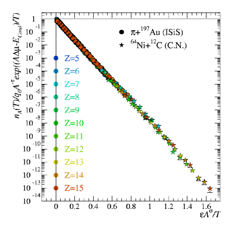
Figure 4: The Fisher scaled yields are plotted versus the scaled temperature for the indicated reactions.

For our third and final demonstration, we show the results of a consistent fit of the ISiS data Elliott et al. (2002a) and of the low energy compound nucleus data Fan et al. (2000) with the Fisher model modified for Coulomb (Eq. (1)). The resulting Fisher scaling is shown in Fig. 4 for both systems. A smooth, continuous behavior is observed from the compound nucleus data up to the higher energy systems. This smooth behavior using a consistent set of Fisher parameters indicates a natural extension of the compound nuclear decay mechanism up to higher energies.

In conclusion, the ISiS data as well as low energy compound nucleus data contain the signature of a liquid to vapor phase transition via their strict adherence to Fisher’s model. Through a direct examination of the mean emission times of the ISiS fragmentation reactions, we infer a stochastic, thermal emission scenario consistent with complex fragment emission at much lower excitation energies.