Critical exponents and phase transition in gold nuclei fragmentation at energies 10.6 and 4.0 GeV/nucleon

Abstract

An attempt to extract critical exponents $\gamma$, $\beta$ and $\tau$ from data on gold nuclei fragmentation due to interactions with nuclear emulsion at energies 4.0 A GeV and 10.6 A GeV is presented. Based on analysis of Campi’s 2nd charge moments, two subsets of data at each energy are selected from the inclusive data, corresponding to ’liquid’ and ’gas’ phases. The extracted values of critical exponents for the selected data sets are in agreement with predictions of ’liquid-gas’ model of phase transition.

, ,

1 Introduction

Multifragmentation, a breakup of an excited nucleus into many intermediate mass fragments, has been discussed for almost twenty years in terms of statistical mechanics; possible critical behavior was investigated. In its ground state nuclear matter behaves like a liquid. Mean field theory simulations [1] predict that nuclear equation of state resembles that of Van der Waals gas. Therefore existence of phase transition, spinodal instabilities and critical point are expected. However, nature of the possible phase transition is still under debate. Existing experimental data do not lead to a conclusive answer [2, 3, 4, 5].

In many papers it was shown (e.g.[3]) that nuclear interactions undergo two stages. During the first stage, prompt nucleons are emitted from the colliding system and they carry out a large amount of available kinetic energy. They result from quasi-elastic and nonelastic collisions of projectile and target nucleons. Immediately after the collision, the remnant of the nucleus is in an excited state with temperature $T_{i}$. At the second stage, the excited remnant expands and cools evolving into neighborhood of the critical point on the temperature–density plane [6]. Then the hot and decompressed nucleon gas with temperature $T_{f}$ condenses into many fragments. This last process is the multifragmentation. It was also shown that total charged fragment multiplicity is proportional to the temperature of the colliding system, both to $T_{i}$ and $T_{f}$ [6].

In the 90-ties there were many attempts to extract critical exponents in nuclear fragmentation from the experimental data, e.g. [7, 8, 9, 10]. A method of charged moments invented by Campi [11] and supported by percolation theory [13] was commonly applied. These attempts did not take into account the fact that it is only the remnant of the nucleus that undergoes multifragmentation process, so all prompt particles (participating in the nucleus-nucleus collision) were included in the analysis. This approach raised a critique [14, 15], that pointed out that: inclusion of prompt particles, assumption that fragment multiplicity is directly proportional to the temperature of the fragmenting system and using fragment charges $Z_{i}$ instead of fragment masses $A_{i}$ are not justified and can significantly change the resulting values of critical exponents.

Recently, the EOS collaboration [16] calculated critical exponents based on a high-statistics sample of fully reconstructed events from fragmentation of Au nuclei with energy 1.0 GeV/nucleon, taking into account the above criteria and using fragment masses, not charges. The obtained results are in agreement with the previously extracted values of the critical exponents [7]. Therefore the exclusion of prompt particles and performing analysis based on moments of mass distribution, instead of charge distribution, does not impact resulting values. This can be understood based on the fact that a large majority of prompt particles are fragments with charge $Z=1$. Their impact on the second charge moments (that take square of the charges) is much smaller than that of heavier fragments.

In this paper we present the analysis of data coming from interactions of projectile gold nuclei of primary energies 4.0 and 10.6 GeV/nucleon with nuclear emulsion target.

2 The experiment

Stacks of BR-2 emulsion pellicles were irradiated with gold ion beam at the AGS accelerator at Brookhaven National Laboratory. The stacks were oriented so that the beam was parallel to the pellicles. Interactions were found during a microscope scanning along the primary tracks in order to obtain a sample with minimum detection bias. The two data sets consist of 448 events at 4.0 GeV/nucleon and 884 events at 10.6 GeV/nucleon. In each event analyzed, multiplicities and emission angles of all produced particles and fragments of colliding nuclei were measured. In addition, charges of projectile nucleus fragments were determined. Singly-charged particles (released protons and produced pions) were distinguished unambiguously from heavier fragments. Charges of heavier fragments ($Z\geq 2$) of the projectile were measured using a photometric method with a CCD camera [17].

The experimental method of identification of prompt particles (i.e. nucleons directly participating in the collision) in emulsion experiments is not available. We can however estimate the number of prompt particles as a difference between the total number of emitted protons $N_{prot}$ and the number of spectator protons $N_{spec}$. $N_{prot}$ is determined using charge balance of the projectile fragments. We have estimated $N_{spec}$ as the number of singly charged particles that are emitted at the angle $\theta<2\theta_{0}$, where $\theta_{0}$ is the average proton emission angle given by relation $\theta_{0}=0.12/p$, and $p$ is the momentum of the nucleon prior to emission [18].

In this paper critical exponents were extracted using the Campi’s charge moments method. The charge moments in our analysis were calculated in two different ways. One of them is to find non-normalized charge moments taking into account all heavy ($Z>2$) fragments, alpha particles and protons emitted from the vertex of interaction following Gilkes at al [7]. The other way is for normalized charge moments and excludes prompt protons following Elliott et al. [16]. The two ways were used to detect possible inconsistencies coming from the choice of the method.

3 Charge moments

Following Campi [11, 12], we define the total charged fragment multiplicity $m$, as $m=N_{f}+N_{\alpha}+N_{prot}$, where $N_{f}$ denotes the number of fragments with charge $Z\geq 3$, $N_{\alpha}$ is the number of emitted alpha particles and $N_{prot}$ is the number of emitted protons.

The distance from the critical point for a given event can be properly measured by a difference between multiplicity $m$ and the multiplicity at the critical point $m_{c}$. The validity of this assumption rests on a linear dependence between temperature of the system $T$ and the total multiplicity $m$, that was shown to be valid by Hauger at al. [3]. Therefore we introduce variable $\epsilon$:

$$\epsilon=m-m_{c},$$ (1)

Fragments of a given charge, $Z_{f}$, were counted on event-by-event basis to determine fragment charge distributions $N_{Z_{f}}$. The normalized charge distribution was defined as $n_{Z_{f}}=N_{Z_{f}}/Z_{A_{0}}$, where $Z_{A_{0}}$ is charge of the nucleus remnant undergoing fragmentation, given by a sum of charges of all fragments $Z_{f}\geq 2$ plus total charge of spectator protons.

In order to compare our results with theoretical calculations (the Fisher model), mass distributions should be used and should be normalized to the remnant mass $A_{0}$ rather than to its charge $Z_{A_{0}}$. In emulsion experiments, fragment mass is not measurable; therefore it was assumed that fragment charge $Z_{f}$ is proportional to its mass $A_{f}$. It was also assumed that on average, charge and mass distributions are equal $N(Z_{f})=N(A_{f})$. In fact, the same assumption is made also by other authors, at least in specific ranges of charges. This is dictated by the difficulty in measuring masses of all heavier fragments emerging from the interaction vertex. In case of electronic experiments masses of fragments only in some small mass range are measured. Therefore, we have to rely on the assumption of proportionality between mass and charge.

Following Campi [11], we define the k-th moment of charge distribution as:

$$M_{k}(\epsilon)=\sum n_{Z_{f}}(\epsilon)Z_{f}^{k},$$ (2)

where the sum extends over all charged fragments except prompt protons in the ’gas phase’, that is for $\epsilon>0$. In the ’liquid phase’,where $\epsilon<0$, in addition the fragment with highest charge $Z_{max}$ is omitted from summation. The above procedure is motivated by the Fisher model. The bulk liquid of infinite volume is excluded from calculation on the ’liquid’ phase. Similar procedure is carried out in percolation models, where percolating cluster of infinite size is excluded from calculation on the ’liquid’ phase.

With the above assumptions, and based on the Fisher model, in the thermodynamic limit the following relations are valid [16]:

$$M_{2}(\epsilon)\sim|\epsilon|^{-\gamma},$$ (3)

$$n_{Z_{f}}(\epsilon)\sim Z_{f}^{-\tau}\;\;\mbox{for}\;\;\epsilon=0$$ (4)

In addition, Bauer et al [19] have shown that:

$$Z_{max}(\epsilon)\sim\epsilon^{\beta}\;\;\mbox{for}\;\;\epsilon<0,$$ (5)

In these equations $\beta$, $\gamma$ and $\tau$ are the critical exponents. $Z_{max}(\epsilon)$ is the average charge of the largest fragment for a given value of the distance from critical point $\epsilon$. The above relations are valid in the neighborhood of the critical point. Far away from the critical point, the behavior of the system is dominated by the mean field regime and these relations are not followed. Very close to the critical point, on the other hand, finite size effects come into play and $M_{2}$ does not raise to infinity with $\epsilon$ approaching 0 (Equation 3), but achieves some maximum value. The critical exponents $\beta$, $\gamma$ and $\tau$ are not independent. A scaling relation between them exists:

$$\tau=2+\frac{\beta}{\beta+\gamma}$$ (6)

Practical calculations of the moments of charge distributions were based on averaging in the small bins of multiplicity $m$ of event-by-event distributions [16, 7]:

$$\langle M_{k}(\epsilon)\rangle=\frac{1}{N}\sum M_{k}^{i}(\epsilon)=\frac{1}{N}\sum_{i}(\sum_{Z_{f}}n_{Z_{f}}^{i}(\epsilon)Z_{f}^{k})$$ (7)

where $i$ is the index of an event, $N$ denotes the total number of events in a given small range of $\epsilon$, $M_{k}^{i}$ is a charge distribution moment for event $i$.

4 Fluctuations close to the critical point

One of the basic effects of the second order phase transition is the appearance of significant fluctuations in the neighborhood of the critical point, in a small range of temperatures $T$ (or other parameter measuring distance from the critical point). Fluctuations grow as the critical point is approached and appear at increasingly large scales. In the case of a normal liquid, the effect is known as the critical opalescence: fluctuations of density of the liquid and sizes of gas bubbles result from vanishing latent heat of the phase transition as the critical point is approached. In the Fisher model of nuclear fragmentation, this is reflected by the divergence of the isothermal compressibility $\kappa_{T}$ at the critical temperature $T_{c}$: small variations of the pressure result in big density changes. In the neighborhood of the critical point, the volume and surface terms of the Gibbs free energy of fragment formation vanish and the fragment distribution is dominated by the power law of Equation 4 [20].

In case of multifragmentation, fluctuations can be analyzed using moments of charge distributions. Campi suggested a variable $\gamma_{2}$ linearly dependent on variance $\sigma^{2}$ of the charge $\langle Z\rangle$ distribution:

$$\gamma_{2}=\frac{M_{2}M_{0}}{M_{1}^{2}}=1+\frac{\sigma^{2}}{\langle Z\rangle^{2}},$$ (8)

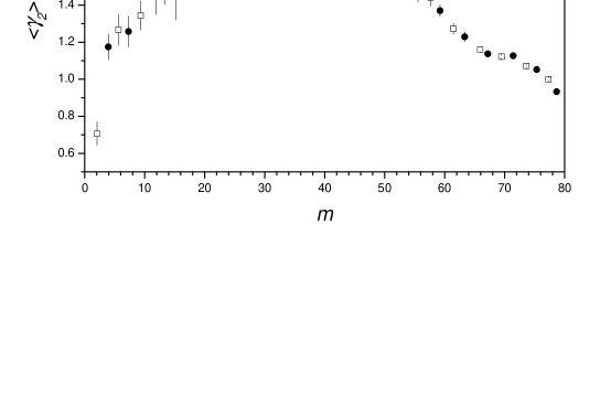
Figure 1: $\langle\gamma_{2}\rangle$ as a function of total charged fragment multiplicity $m$ at energies 4.0 and 10.6 GeV/nucleon. The error bars show the dispersion of $\gamma_{2}$ in each bin.

Figure 1 shows $\langle\gamma_{2}\rangle$ as a function of multiplicity $m$ for energies 4.0 and 10.6 GeV/nucleon. As critical value of multiplicity $m_{c}$ is not identified at this stage, in all above calculations charge moments were calculated with $Z_{max}$ excluded. For multiplicities smaller than $m\simeq 30$, $\langle\gamma_{2}\rangle$ grows monotonically with multiplicity, for multiplicities larger than $m\simeq 40$, it falls down monotonically. Fluctuations of $\gamma_{2}$, reflected in large dispersion, are largest for multiplicities between $10$ and $40$. It is commonly assumed that strong maximum of $\langle\gamma_{2}\rangle$ results from undergoing a phase transition at critical point multiplicity $m=m_{c}$. The region of multiplicities $m<m_{c}$ is called a ’liquid’ phase, and events with $m>m_{c}$ are called to be in ’gas’ phase. However, the presence of maximum of $\langle\gamma_{2}\rangle$ is not a conclusive argument for appearance of phase transition. It was shown [16] that such maximum is observed also in systems that do not undergo a phase transition. Therefore Figure 1 will be treated as only a hint for possibility of phase transition in a specific range of multiplicities. It is also worth mentioning that $\gamma_{2}$ fluctuations at energies 4.0 and 10.6A GeV agree well with each other.

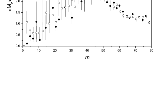
Figure 2: Mean value of the second charge moment $\langle M_{2}\rangle$ as a function of multiplicity $m$ for energies 4.0 and 10.6 GeV/nucleon. The error bars show dispersion of $M_{2}$ values for each bin.

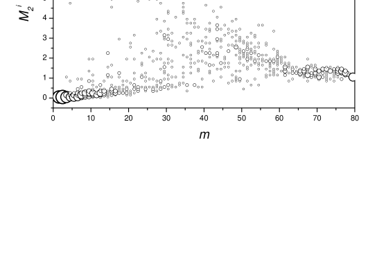
Figure 3: Scatter plot of second charge moments for individual events $M_{2}^{i}$ as function multiplicity $m$ for energy 10.6 GeV/nucleon.

In order to closer analyze the fluctuations, the mean values of second moment of charge distribution $\langle M_{2}\rangle$ were plotted versus multiplicity in Figure 2. Similar characteristics to that of $\langle\gamma_{2}\rangle$ is seen. Large dispersion of $M_{2}$, especially in the ’liquid’ phase reflects strong fluctuations of experimental values.

Figure 3 shows a scatter plot of second charge moments for individual events $M_{2}^{i}$ versus multiplicity $m$ at energy 10.6 GeV/nucleon. Strong fluctuations of $M_{2}^{i}$ for multiplicities $15\leq m\leq 45$ are clearly visible, which result in large dispersion of $M_{2}$ values (shown as error bars in Figure 2). For systems undergoing a second order phase transition, it is expected that fluctuations rise in the neighborhood of the critical point. Therefore observation of large fluctuations quite far away from expected critical region should be attributed to a different physical phenomenon. For example, events with values of $M_{2}^{i}>4$ and multiplicity $m<20$ are fission-like (only 2 heavy fragments plus alphas and protons). Two distinct groups of experimental points are seen in Figure 3. One of these groups consists of events with multiplicity smaller than $m=35$ and $M_{2}<0.9$, the other — of events with multiplicities larger than $m=30$ and largest $M_{2}$ values for a given $m$. The former group, with small multiplicities and small $M_{2}^{i}$ suggests that the fragment charge distribution must be dominated by one heavy fragment – i.e. the expected characteristics of the ’liquid’ phase. On the other hand, the latter group of events, with large multiplicity and larger $M_{2}$, suggests existence of a larger number of small fragments, thus it resembles the expected characteristics of the ’gas’ phase. The events which do not belong to either of these groups may be thought of as nuclei in a ’mixed’ phase (see Section 7). The ’liquid’ and ’gas’ groups were selected from experimental data for further analysis. Figure 4 shows the selection criteria. The ’liquid’ group of events consist of those with multiplicity smaller than $m=35$ located below the solid line, while the ’gas’ group consists of events with $m>30$ and located above and to the right of the dashed line. Similar selection was performed for data with energy 4.0 GeV/nucleon – see Figure 5.

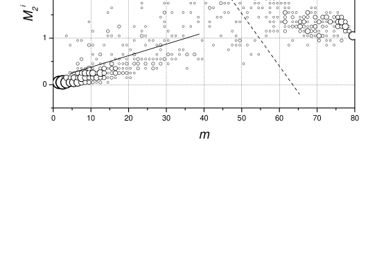
Figure 4: Selection of ’liquid’ and ’gas’ groups of events in the $M_{2}^{i}$—$m$ scatter plot.

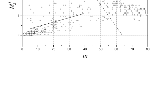
Figure 5: Second charge moment $M_{2}^{i}$ for individual events vs. multiplicity $m$ for energy 4.0 GeV/nucleon. Events selection criteria .

Let us look at these two selected groups in order to check if they really can be treated as ’liquid’ and ’gas’ phases. For example, Figure 6 presents charge distributions as a function of heavy ($Z>2$) fragment multiplicity, $N_{f}$, for the two selected groups of data. Fragment charge distributions are clearly different in both groups. The charge distribution for the group of low multiplicity events consists mainly of events with one heavy fragment emitted ($Z\geq 45$). If the second fragment is emitted, it has a small charge ($Z\leq 3$). Therefore, we will refer to this group of data as ’liquid’ as for these events one large fragment remains after collision in analogy to the large drop of liquid. In most cases there are only alphas and protons accompanying the large heavy fragment. The second group of events has totally different charge distribution that consists of events with number of emitted heavy fragments ranging from 1 to 9 and charges of fragments $Z\leq 25$. The majority of fragments in this group has charges $Z\leq 15$. We will call this group of events a ’gas’ as it consists of events with many light fragments emitted. The analysis presented in subsequent sections presents results on these selected sets of data unless explicitly stated otherwise.

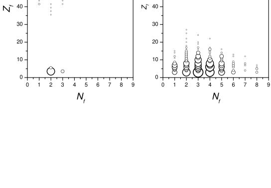
Figure 6: Charge distributions in events with different heavy fragment multiplicity $N_{f}$ for the two selected groups of experimental data at energy 10.6 GeV/nucleon.

5 Critical exponent $\gamma$

In order to extract the critical exponent $\gamma$ and the critical value of multiplicity $m_{c}$ the method known as ’gama matching’ was used [19, 16]. The outline of this method is the following. A trial value of the critical multiplicity $m_{c}$ is chosen. For a given $m_{c}$, a distribution of mean values of the moment $\langle M_{2}(\epsilon)\rangle$ is determined as a function of distance from the critical point $\epsilon=m-m_{c}$. Then the ranges in $\epsilon$ are chosen to fit the power law (3) to the experimental data, separately for the ’gas’ and ’liquid’ phases. With fitting boundaries determined, the linear fit to the $ln\langle M_{2}(\epsilon)\rangle$ versus $ln|\epsilon|$ is made to extract values of the slope $\gamma$ separately for ’gas’ and ’liquid’ phases.

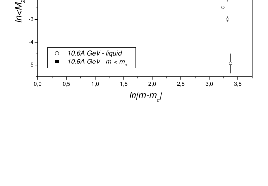
Figure 7: Mean value of second charge moment $\langle M_{2}\rangle$ for a ’liquid’ phase as a function of multiplicity $m$ for energy 10.6 GeV/nucleon. Full squares show data for all events with $m<m_{c}$, open squares represent data for selected ’liquid’ events only. The line shows the fit used to determine critical exponent $\gamma$.

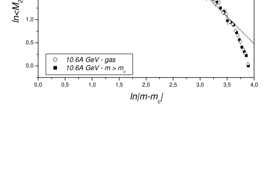
Figure 8: Mean value of second charge moment $\langle M_{2}\rangle$ for a ’gas’ phase as a function of multiplicity $m$ for energy 10.6 GeV/nucleon. Full squares show data for all events with $m>m_{c}$, open squares represent data for selected ’gas’ events only. Plotted lines show fits to the ’gas’ data (solid line) and $m>m_{c}$ data (dotted line).

The fitting boundaries for the ’liquid’ phase are easily determined. Figure 7 presents a comparison of second moments of charge distribution for the selected ’liquid’ phase and all available experimental data at $m<m_{c}$. It is seen that the selection results in appearance of a very clear region of power law dependence.

Similar comparison for the ’gas’ phase is shown in Figure 8. The impact of selection of the ’gas’ phase is not significant in this case. The region of the power law dependence is not clearly seen. This may be due to the inclusion of the charge of the largest fragment $Z_{max}$ in the ’gas’ phase. The largest charge dominates the second moment, shifts it to the higher values and makes the power law less visible, probably due to the finite size effect. Thus, it may be interesting to check if the exclusion of $Z_{max}$ also in the ’gas’ phase reveals a clear range of power law dependence of $<M_{2}>$ versus $\epsilon$. The $M_{2}$ moment for the ’gas’ phase computed without $Z_{max}$ is shown in Figure 9. Open circles represent moments computed for ’gas’ group of data, filled circles represent those for all experimental data at $m>m_{c}$, without selection. In both cases the region of power law behavior is now clearly visible. This region is much larger for selected ’gas’ data compared to $m>m_{c}$ data, so it is now clear in which region of $\epsilon$ the fit should be performed. In other words, Figure 9 was used as a guideline in determining fitting region in the ’gas’ phase in the ’gamma matching procedure’. It is interesting that the value of $\gamma_{gas}=1.14\pm 0.05$ determined from moments of charge distribution with $Z_{max}$ excluded is very close to the value determined by the ’gamma matching procedure’ (i.e. with $Z_{max}$ included).

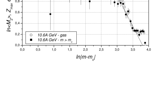
Figure 9: Mean value of the second charge moment $\langle M_{2}\rangle$ for a ’gas’ phase with exclusion of the largest charge $Z_{max}$ as a function of multiplicity $m$ for energy 10.6 GeV/nucleon.

The above procedure was repeated for several trial values of the critical point $m_{c}$. The value of the critical exponent $\gamma$ and critical point $m_{c}$ is found by demanding that $|\gamma_{gas}-\gamma_{liquid}|$ takes a minimum value and $\gamma_{gas}$ and $\gamma_{liquid}$ agree with each other within statistical errors. Trial values of the critical point were selected in the range $25\leq m_{c}\leq 35$.

Table 1: Critical exponent $\gamma$ for ’gas’ and ’liquid’ phases for different choices of trial value of critical point $m_{c}$ for energy 10.6 GeV/nucleon used in gamma matching procedure. Normalized moments

trial $m_{c}$	$\gamma_{liquid}$	$\gamma_{gas}$	$|\gamma_{liquid}-\gamma_{gas}|$
$26$	$0.80\pm 0.00$	$1.45\pm 0.06$	$0.63\pm$ 0.10
$28$	$0.96\pm 0.11$	$1.32\pm 0.05$	$0.35\pm 0.12$
$29$	$1.04\pm 0.11$	$1.26\pm 0.05$	$0.22\pm 0.12$
$30$	$1.12\pm 0.12$	$1.20\pm 0.05$	$0.08\pm 0.13$
$31$	$1.20\pm 0.13$	$1.14\pm 0.05$	$0.05\pm 0.14$
$32$	$1.27\pm 0.14$	$1.08\pm 0.05$	$0.19\pm 0.15$
$34$	$1.42\pm 0.15$	$0.96\pm 0.04$	$0.46\pm 0.16$

Table 2: Critical exponent $\gamma$ for ’gas’ and ’liquid’ phases for different choices of trial value of critical point $m_{c}$ for energy 10.6 GeV/nucleon used in gamma matching procedure. Non-normalized moments.

trial $m_{c}$	$\gamma_{liquid}$	$\gamma_{gas}$	$|\gamma_{gas}-\gamma_{liquid}|$
$26$	$0.78\pm 0.07$	$1.30\pm 0.11$	$0.48\pm$ 0.13
$28$	$0.93\pm 0.09$	$1.22\pm 0.10$	$0.20\pm 0.14$
$29$	$1.02\pm 0.10$	$1.17\pm 0.10$	$0.15\pm 0.14$
$30$	$1.09\pm 0.10$	$1.13\pm 0.10$	$0.03\pm 0.14$
$31$	$1.17\pm 0.10$	$1.08\pm 0.10$	$0.09\pm 0.14$
$32$	$1.24\pm 0.12$	$1.03\pm 0.09$	$0.21\pm 0.14$
$34$	$1.39\pm 0.13$	$0.94\pm 0.08$	$0.45\pm 0.15$

Table 3: Critical exponent $\gamma$ for ’gas’ and ’liquid’ phases for different choices of trial value of critical point $m_{c}$ for energy 4.0 GeV/nucleon used in gamma matching procedure. Normalized moments.

trial $m_{c}$	$\gamma_{liquid}$	$\gamma_{gas}$	$|\gamma_{gas}-\gamma_{liquid}|$
$26$	$0.83\pm 0.09$	$1.32\pm 0.09$	$0.49\pm 0.13$
$28$	$1.01\pm 0.11$	$1.22\pm 0.09$	$0.21\pm 0.14$
$29$	$1.10\pm 0.12$	$1.17\pm 0.08$	$0.08\pm 0.14$
$30$	$1.18\pm 0.13$	$1.12\pm 0.08$	$0.06\pm 0.14$
$31$	$1.27\pm 0.14$	$1.07\pm 0.08$	$0.20\pm 0.15$
$32$	$1.35\pm 0.15$	$1.01\pm 0.07$	$0.33\pm 0.16$
$34$	$1.52\pm 0.16$	$0.91\pm 0.07$	$0.61\pm 0.17$

Table 4: Critical exponent $\gamma$ for ’gas’ and ’liquid’ phases for different choices of trial value of critical point $m_{c}$ for energy 4.0 GeV/nucleon used in gamma matching procedure. Non-normalized moments.

trial $m_{c}$	$\gamma_{liquid}$	$\gamma_{gas}$	$|\gamma_{gas}-\gamma_{liquid}|$
$26$	$0.77\pm 0.07$	$1.53\pm 0.08$	$0.75\pm 0.11$
$28$	$0.96\pm 0.08$	$1.42\pm 0.07$	$0.46\pm 0.11$
$29$	$1.05\pm 0.09$	$1.36\pm 0.07$	$0.31\pm 0.11$
$30$	$1.13\pm 0.09$	$1.30\pm 0.07$	$0.17\pm 0.11$
$31$	$1.22\pm 0.09$	$1.24\pm 0.07$	$0.02\pm 0.11$
$32$	$1.30\pm 0.10$	$1.18\pm 0.06$	$0.13\pm 0.12$
$34$	$1.47\pm 0.11$	$1.06\pm 0.06$	$0.41\pm 0.14$

Results of the calculations for energy 10.6 GeV/nucleon are presented in Tables 1 and 2. Table 1 shows results obtained based on normalized charge distribution moments whereas Table 2 present results from calculation based on non normalized moments. It is easily seen that both procedures give exponents that agree with each other within statistical errors. Final value of exponent $\gamma$ is calculated as a mean value of $\gamma_{gas}$ and $\gamma_{liquid}$ for normalized moments. The critical point is determined at $m_{c}=31\pm 2$ and the critical exponent $\gamma=1.17\pm 0.09$.

The analogous results of the ’gama matching’ procedure for energy 4.0 GeV/nucleon are given in Tables 3 and 4. The determined critical point is $m_{c}=30\pm 2$ and the critical exponent $\gamma=1.15\pm 0.09$. Figure 10 shows values of $|\gamma_{liquid}-\gamma_{gas}|$ plotted as a function of trial values of critical multiplicity at energy 10.6 Gev/nucleon. Figure 11 presents results of fitting procedure for $\gamma_{liquid}$ and $\gamma_{gas}$ for critical multiplicity value $m_{c}=30$ for the same energy.

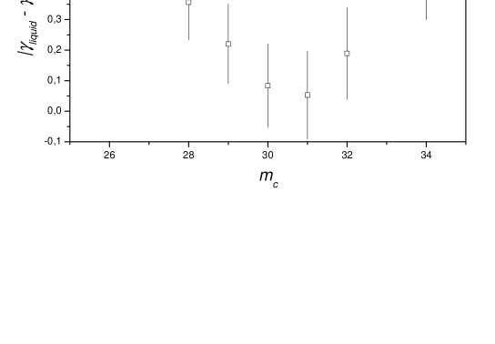
Figure 10: Difference $|\gamma_{liquid}-\gamma_{gas}|$ as a function of trial multiplicity $m_{c}$ for energy 10.6 GeV/nucleon.

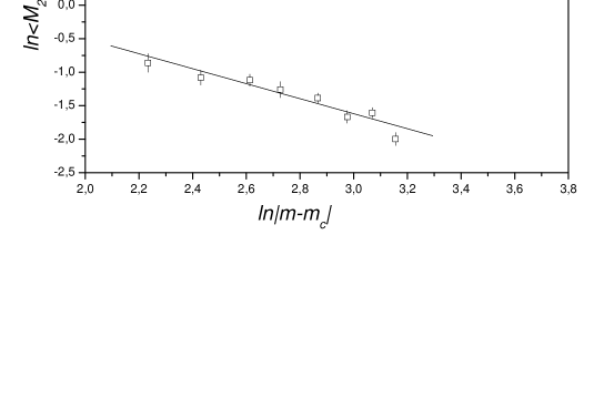
Figure 11: Mean value of second charge moment $\langle M_{2}\rangle$ for a ’liquid’ and ’gas’ as a function of multiplicity $m$ for energy 10.6 GeV/nucleon. The plotted lines show fits to experimental data used to determine critical exponent $\gamma$.

6 Critical exponents $\beta$ and $\tau$

After determination of the critical multiplicity $m_{c}$ and ranges of $\epsilon$ in which to fit the critical exponents, determination of the exponents $\beta$ i $\tau$ is straightforward. Based on Equation 5, the mean value of $\ln Z_{max}$ was plotted as a function of $\ln|m-m_{c}|$ (Figure 12). The slope of the linear fit to the plotted relation gives the critical exponent $\beta$. A linear fit was made within the fitting boundaries determined during the ’gamma matching procedure’. For energy 10.6 GeV/nucleon the determined value of $\beta=0.33\pm 0.01$ with $\chi^{2}/ndf=1.66$, and for 4.0 GeV/nucleon $\beta=0.34\pm 0.01$ with $\chi^{2}/ndf=0.99$.

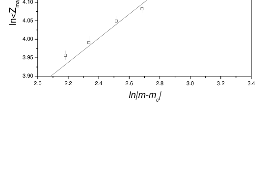
Figure 12: Mean Value of $ln\langle Z_{max}\rangle$ as a function of distance from critical point $\epsilon$ for ’liquid’ phase 10.6 GeV/nucleon.

The critical exponent $\tau$ was determined from equation [7, 16]:

$$\frac{\Delta\ln\langle M_{3}\rangle}{\Delta\ln\langle M_{2}\rangle}=\frac{\tau-4}{\tau-3}.$$ (9)

Figure 13 presents $\ln\langle M_{3}\rangle$ versus $\ln\langle M_{2}\rangle$ for the ’gas’ phase at energy 10.6 GeV/nucleon together with the linear fit. The slope of this linear fit is used to determine the $\tau$ exponent, which is $\tau=2.11\pm 0.05$ for 10.6 GeV/nucleon and $\tau=2.12\pm 0.04$ for energy 4.0 GeV/nucleon. To verify the consistency, the exponent $\tau$ also was determined from Equation 4. This Equation is supposed to be valid at the critical point, but in order to have sufficient statistics, data with $25<m<35$ were used. Normalized charge multiplicity distribution was calculated and plotted in Figure 14. The exponent $\tau$ is given by the slope of the linear fit to the data points for charges from $Z=6$ to $Z=16$. For charges smaller than 6, the assumptions of the Fisher model are not valid [22] and for charges larger than 16 experimental data statistics is too small. The resulting value $\tau=2.19\pm 0.33$, with reduced $\chi^{2}=1.2$ is in agreement with previously determined value.

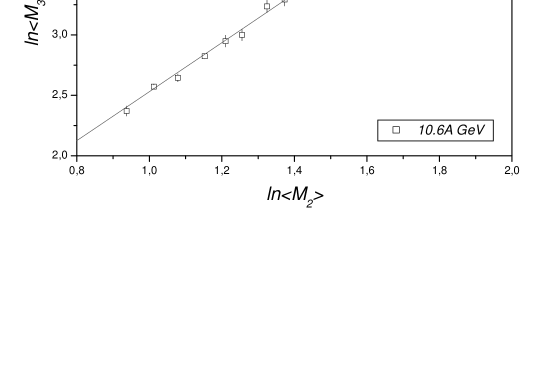
Figure 13: Relation between charge moments $\ln\langle M_{3}\rangle$ and $\ln\langle M_{3}\rangle$ for gas phase 10.6 GeV/nucleon.

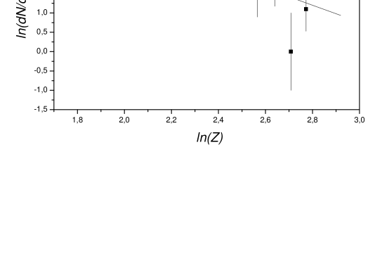
Figure 14: Normalized charge distribution for event with multiplicity $m$ within a range $25<m<35$.

7 Discussion

Table 5 summarizes the determined values of critical exponents $\gamma$, $\beta$ and $\tau$ at energies 4.0 and 10.6 GeV/nucleon both for normalized and non-normalized charge moments. For comparison, exponents obtained by the EOS, EMU01 and KLMM experiments are also shown, as well as the values predicted by the liquid-gas and percolation models. The data on the $\beta$ and $\gamma$ exponents from Table 5 are plotted in Figure 15. The values of $\beta$ and $\gamma$ exponents determined in this work are very close to those expected for the ’liquid-gas’ phase transition, both for 4.0 and 10.6 GeV/nucleon data. We note that the critical exponents discussed here were determined from the selected ’liquid’ and ’gas’ groups of events. Earlier analyses, without such a selection, gave values of the exponents which do not agree with any of the models.

Values of the critical exponent $\tau$ predicted by the percolation and liquid-gas models are not too different. As experimental errors are large compared to the difference between the predicted values of $\tau$, this exponent cannot be used to discriminate models of multifragmentation.

Table 5: Critical exponents $\gamma$, $\beta$, $\tau$ for energy 4.0 GeV/nucleon and 10.6GeV/nucleon

$Data$	$\gamma$	$\beta$	$\tau$
Au-Em 4.0A GeV norm	$1.15\pm 0.09$	$0.34\pm 0.01$	$2.12\pm 0.04$
Au-Em 10.6A GeV norm	$1.17\pm 0.09$	$0.33\pm 0.01$	$2.11\pm 0.05$
Au-Em 4.0A GeV	$1.23\pm 0.09$	$0.36\pm 0.02$	$2.15\pm 0.04$
Au-Em 10.6A GeV	$1.11\pm 0.09$	$0.33\pm 0.02$	$2.16\pm 0.05$
Au-C 1.0A GeV (EOS [16])	$1.40\pm 0.10$	$0.29\pm 0.02$	$2.14\pm 0.06$
Au-Em 10.6A GeV (EMU01 [10])	$0.86\pm 0.05$	$0.25\pm 0.02$	$2.23\pm 0.05$
Au-Em 10.6A GeV (KLMM [8])		$0.19\pm 0.02$	$1.88\pm 0.06$
Liquid-gas model	$1.23$	$0.33$	$2.21$
Percolation model	$1.80$	$0.41$	$2.18$

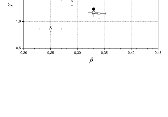
Figure 15: Comparison of determined and predicted values of critical exponent $\gamma$ and $\beta$.

Presented in this work a suggestion that the Fisher’s liquid drop model properly describes multifragmentation process, is in agreement with recently published results of the ISiS collaboration [23], confirming that the Fisher’s scaling law is followed by experimental data. In addition, Mader et al. [24] have shown a similarity between predictions of the Fisher model and clusterisation process in the three-dimensional Ising model. Therefore, multifragmentation can be interpreted in a similar way as condensation of liquid drops in equilibrium with the bulk liquid.

One can try to estimate a critical temperature of the system by using a relation between multiplicity and temperature of the system given in [3, 6]. Estimation of the initial temperature of the system after collision, $T_{i}$, was based on Fermi gas model and does not take into account the expansion of the system. The final temperature of the system at breakup, $T_{f}$, was estimated based on a relation between multiplicity $m$ and temperature $T$ for isotopic-yield-ratio thermometer given in [3]. Our values of critical multiplicity ($m_{c}=30$ and $m_{c}=31$ at 4.0 and 10.6 GeV/nucleon, respectively) correspond to $T_{i}=9.3\pm 0.7$ MeV and $T_{f}=5.4\pm 0.2$ MeV. The error of $T_{i}$ reflects uncertainty of the input parameters in the Fermi gas model. These $T_{i}$ and $T_{f}$ values bracket the critical temperature of the system. This estimated range for the critical temperature agrees with predictions of the Fisher model if we take into account the scaling of critical temperature with the finite system size [16]. The estimation of the critical temperature relies on the assumption that relation between multiplicity $m$ and temperature of the system established for energy 1.0 A GeV applies also for higher energies 4.0 and 10.6 GeV/nucleon.

The above results, together with results of ISiS collaboration [23] suggest that not all multifragmentation events undergo a second order phase transition. The data excluded from our analysis presented above may be interpreted as events in which multifragmentation occurs far away from the critical point. These events could undergo a first order phase transition so that ’gas’ and ’liquid’ coexist inside the nucleus as suggested by experimental analysis of GSI data [2].

As noted earlier, the excited nucleus after a collision evolves into the neighborhood of the critical point on the density–temperature plane. If multifragmentation occurs close to the critical point, critical exponents characterizing second order phase transition occurring in the neighborhood of the critical point should be observed. If for some events multifragmenation occurs far away from the critical point and they are included in the analysis, the observed values of critical exponents could be altered so that the whole picture of the physical process is obscured. In such situations proper selection of events should help obtain true values of critical exponents.

Events excluded from our analysis show very strong fluctuations of the second moment of the charge distribution significantly far away from the critical point, especially in the liquid phase. Large fluctuations could result from coexistence of two different phases with different properties inside a single nucleus. Below critical multiplicity $m_{c}$ (proportional to temperature of the system) two separate phases with significantly different properties could coexist in nucleus as is suggested by mean field [25, 26, 1] or canonical model calculations [27]. The coexistence of the two phases may take place in wide ranges of temperature and pressure. This could explain large fluctuations of second moment of charge distribution far away from the critical point. It is also important to stress that moment $M_{2}$ is proportional to the isothermal compressibility of the system. Therefore, large fluctuations of $M_{2}$ correspond to fluctuations of the compressibility $\kappa_{T}$ and to fluctuation of the density of the system. Large fluctuations of $M_{2}$ observed in ’liquid phase’ (Figure 3) may be interpreted as resulting from large density difference between the two coexisting phases.

In summary, an attempt to extract critical exponents $\gamma$, $\beta$ and $\tau$ was performed, using data coming from interactions of gold nuclei with nuclear emulsion at energies 4.0 A GeV and 10.6 A GeV. To extract the exponents, two subsets of data with characteristics similar to that of ’gas’ and ’liquid’ phases were selected, based on analysis of Campi’s 2nd charge moments. The extracted values of the critical exponents for the selected data sets are in agreement with predictions of liquid-gas model of phase transition. The same analysis performed without the selection of ’gas’ and ’liquid’ samples favors neither percolation nor liquid-gas model of phase transition. A suggestion is made that data excluded from the above mentioned samples represents events where phase transition, if any, occurs far from the critical point.

References

- [1] T. Sil et al, Phys. Rev. C 62, 064603 (2000)
- [2] J. Pochodzalla et al., Phys. Rev. Lett. 75, 1040 (1995)
- [3] J. Hauger et al. , Phys. Rev. Lett. 77, 235 (1996)
- [4] R. Nebauer and J. Aichelin, Nucl. Phys. A681, 353 (2001)
- [5] M. Kleine Berkenbusch et al., Phys. Rev. Lett. 88, 022701 (2002)
- [6] J.A. Hauger et al., Phys. Rev. C57, 764 (1998)
- [7] M.L. Gilkes et al., Phys. Rev. Lett. 73, 1590 (1994)
- [8] M.L. Cherry et al., Phys. Rev C52 2652 (1995)
- [9] M.I. Adamovitch. et al., Eur Phys J. A 1, 77 (1998)
- [10] M.I. Adamovitch. et al., Eur Phys J. A 5, 429 (1999)
- [11] X. Campi, J. Phys. A19, L917 (1986)
- [12] X. Campi, Phys. Lett. B208, 351 (1988)
- [13] D. Stauffer and A. Aharony, ”Introduction to Percolation Theory”, 2nd ed. (Taylor and Francis, Lonfon 1992)
- [14] W. Bauer and W.A. Friedman, Phys. Rev. Lett. 75, 768 (1995)
- [15] M.L. Gilkes et al., Phys. Rev. Lett. 75, 768 (1995)
- [16] J. B. Elliott, Phys. Rev., C 62, 064603 (2000)
- [17] D. Kudzia et al., Nucl. Inst. Meth. A431, 252 (1999)
- [18] C.F. Powell, P.H. Fowler and D.H. Perkins, The Study of Elementary Particles by the Photographic Method , Pergamon, New York (1959)
- [19] W. Bauer, Phys. Rev. C 38, 1297(1988)
- [20] M.E. Fisher, Physics (N.Y.)3, 255 (1967)
- [21] M.E. Fisher, Rep. Prog Phys. 30, 615 (1969)
- [22] A.D. Panagiotou et al., Phys. Rev. C 31,55-61 (1985)
- [23] J. B. Elliott, Phys. Rev. Lett. 88, 2701 (2002)
- [24] C.M. Mader et al., Preprint arXiv:nucl-th/0103030 (2001)
- [25] J. N. De et al., Phys. Rev. C55, R1641 (1997)
- [26] J.N. De , B.K. Agrawal and S.K. Samaddar, Phys. Rev. C59, R1 (1999)
- [27] S.J. Lee and A.Z. Mekjan , Phys. Rev., C 56 2621(1997)