version 27

for Phys. Rev. C Elliptic flow from two- and four-particle correlations in Au + Au collisions at $\sqrt{s_{NN}}=130$ GeV

Abstract

Elliptic flow holds much promise for studying the early-time thermalization attained in ultrarelativistic nuclear collisions. Flow measurements also provide a means of distinguishing between hydrodynamic models and calculations which approach the low density (dilute gas) limit. Among the effects that can complicate the interpretation of elliptic flow measurements are azimuthal correlations that are unrelated to the reaction plane (non-flow correlations). Using data for Au + Au collisions at $\sqrt{s_{NN}}=130$ GeV from the STAR TPC, it is found that four-particle correlation analyses can reliably separate flow and non-flow correlation signals. The latter account for on average about 15% of the observed second-harmonic azimuthal correlation, with the largest relative contribution for the most peripheral and the most central collisions. The results are also corrected for the effect of flow variations within centrality bins. This effect is negligible for all but the most central bin, where the correction to the elliptic flow is about a factor of two. A simple new method for two-particle flow analysis based on scalar products is described. An analysis based on the distribution of the magnitude of the flow vector is also described.

I INTRODUCTION

In non-central heavy-ion collisions, the initial spatial deformation due to geometry and the pressure developed early in the collision causes azimuthal momentum-space anisotropy, which is correlated with the reaction plane Reis97 ; Herr99 ; OlliQM98 ; Palaiseau . Measurements of this correlation, known as anisotropic transverse flow, provide insight into the evolution of the early stage of a relativistic heavy-ion collision Sorge97 . Elliptic flow is characterized by the second harmonic coefficient $v_{2}$ of an azimuthal Fourier decomposition of the momentum distribution Olli92 ; Volo96 ; Posk98 , and has been observed and extensively studied in nuclear collisions from sub-relativistic energies on up to RHIC. At top AGS and SPS energies, elliptic flow is inferred to be a relative enhancement of emission in the plane of the reaction. Elliptic flow is developed mostly in the first several fm$/c$ (of the order of the size of nuclei) after the collision and thus provides information about the early-time thermalization achieved in the collisions STAR01 . Generally speaking, large values of flow are considered signatures of hydrodynamic behavior Olli92 ; Teaney02 ; Teaney01 although an alternative approach ZiWei02 ; Ko02 ; Molnar ; Zabrodin ; Huma02 is also argued to be consistent with the large elliptic flow for pions and protons at RHIC STAR01b . Models in which the colliding nuclei resemble interacting volumes of dilute gas — the low density limit Heiselberg (LDL) — represent the limit of mean free path that is the opposite of hydrodynamics. It remains unclear to what extent the LDL picture can describe the data at RHIC, and valuable insights can be gained from mapping out the conditions under which hydrodynamic and LDL calculations can reproduce the measured elliptic flow.

Anisotropic flow refers to correlations in particle emission with respect to the reaction plane. The reaction plane orientation is not known in experiment, and anisotropic flow is usually reconstructed from the two-particle azimuthal correlations. But there are several possible sources of azimuthal correlations that are unrelated to the reaction plane — examples include correlations caused by resonance decays, (mini)jets, strings, quantum statistics effects, final state interactions (particularly Coulomb effects), momentum conservation, etc. The present study does not distinguish between the various effects in this overall category, but classifies their combined effect as “non-flow” correlations.

Conventional flow analyses are equivalent to averaging over correlation observables constructed from pairs of particles. When such analyses are applied to relativistic nuclear collisions where particle multiplicities can be as high as a few thousand, the possible new information contained in multiplets higher than pairs remains untapped. A previous study of high-order flow effects focused on measuring the extent to which all fragments contribute to the observed flow signal Jian92 , and amounted to an indirect means of separating flow and non-flow correlations. Given that flow analyses based on pair correlations are sensitive to both flow and non-flow effects, the present work investigates correlation observables constructed from particle quadruplets. The cumulant formalism removes the lower-order correlations which are present among any set of four particles, leaving only the effect from the so-called “pure” quadruplet correlation. The simplest cumulant approach, in terms of both concept and implementation, partitions observed events into four subevents. In the present study, the four-subevent approach is demonstrated, but our main focus is on a more elaborate cumulant method, developed by Borghini, Dinh and Ollitrault Olli00 ; Olli01 . There are indications that non-flow effects contribute at a negligible level to the four-particle cumulant correlationOlli00 ; Olli01 , making it unnecessary to continue to even higher orders for the purpose of separating the flow and non-flow signals. This observation is confirmed by our Monte-Carlo simulations

In this analysis the observed multiplicity of charged particles within the detector acceptance is used to characterize centrality. This leads to some fluctuations of the impact parameter and, correspondingly, of the elliptic flow within each centrality bin, especially in the bin of highest multiplicity. In the present study, a correction is applied to reduce a possible bias in the measurements of the mean elliptic flow due to impact parameter fluctuations in the centrality bins to an insignificant level.

The present study begins with a review of the standard pair correlation method, and provides details concerning the approach adopted in earlier STAR publications STAR01 ; STAR01b for treating non-flow correlations. A new method of pair flow analysis using the scalar product of flow vectors also is introduced. In the conventional method, a flow coefficient is calculated by the mean cosine of the difference in angle of two flow vectors. In the scalar product method, this quantity is weighted by the lengths of the vectors. The new method offers advantages, and is also simple to apply. Also, an analysis in terms of the distribution of the magnitude of the flow vector is discussed.

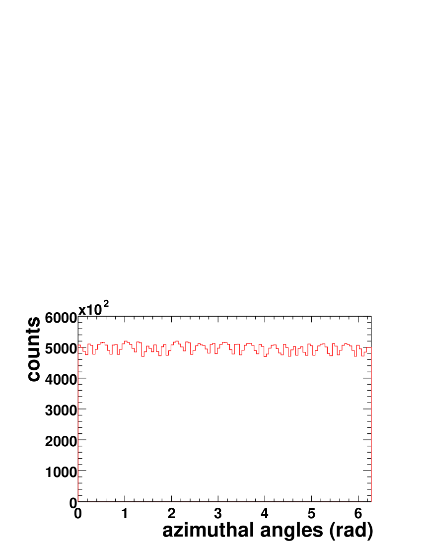
Figure 1: The azimuthal angle distribution of tracks from minimum bias events. Dips are due to the reduced efficiency at sector boundaries of STAR TPC.

Measurements presented in this paper are based on Au+Au data at $\sqrt{s_{NN}}$ = 130 GeV recorded by STAR (Solenoidal Tracker At RHIC) during the summer of 2000. A detailed description of the detector in its year-one configuration can be found elsewhere STAR99 . The main feature of the STAR TPC relevant to this analysis is its full azimuthal coverage (see Fig. 1). The analysis is based on 170000 events corresponding to a minimum bias trigger. Events with a primary vertex beyond 1 cm radially from the beam or 75 cm longitudinally from the center of the Time Projection Chamber (TPC) were excluded. Within the selected events, tracks were used for the estimation of the flow vector if all five of the following conditions were satisfied: they passed within 2 cm of the primary vertex, they had at least 15 space points in the TPC, the ratio of the number of space points to the expected maximum number of space points was greater than 0.52, pseudorapidity $|\eta|<1.3$, and transverse momentum $0.1<p_{t}<2.0$ GeV$/c$. Particles over a wider range in $\eta$ and $p_{t}$ were correlated with this flow vector as shown in the graphs below. Centrality is characterized in eight bins of charged particle multiplicity, $n_{\rm ch}$, divided by the maximum observed charged multiplicity, $n_{\rm max}$, with a more stringent cut $|\eta|<0.75$ imposed only for this centrality determination. The above cuts are essentially the same as used in the previous STAR studies of elliptic flow STAR01 ; STAR01b .

II Two-particle correlation methods

Anisotropic transverse flow manifests itself in the distribution of $\phi^{\prime}=\phi-\Psi$, where $\phi$ is the measured azimuth for a track in detector coordinates, and $\Psi$ is the azimuth of the estimated reaction plane in that event. The observed anisotropies are described by a Fourier expansion,

$$dN/d\phi^{\prime}\propto 1+2v_{1,obs}\cos\phi^{\prime}+2v_{2,obs}\cos 2\phi^{\prime}+...\,.$$ (1)

Each measurable harmonic can yield an independent estimate $\Psi_{n}$ of the event reaction plane via the event flow vector $Q_{n}$:

$$Q_{n}\cos n\Psi_{n} = \sum_{i}\cos n\phi_{i},$$

$$Q_{n}\sin n\Psi_{n} = \sum_{i}\sin n\phi_{i}\,,$$ (2)

where the sums extend over all particles in a given event. The observed values of $v_{n,obs}$ corrected for the reaction plane resolution yield $v_{n}$Posk98 . Below we will also use the representation of the flow vector as a complex number with real and imaginary parts equal to $x$ and $y$ components defined in Eq. (2):

$$Q_{n}=\sum_{i}u_{n,i},$$ (3)

where $u_{n,i}=e^{in\phi_{i}}$ is a unit vector associated with the $i$-th particle; its complex conjugate is denoted by $u_{n,i}^{*}$.

II.1 Correlation between flow angles from different subevents. Estimate of non-flow effects.

In order to report anisotropic flow measurements in a detector-independent form, it is customary to divide each event into two subevents and determine the resolution of the event plane by correlating the $Q_{n}$ vector for the subevents Dani85 ; Posk98 . In order to estimate the contribution from different non-flow effects one can use different ways of partitioning the entire event into two subevents. The partition according to particle charge should be more affected by resonance decay effects because the decay products of neutral resonances have opposite charge. The partition using two (pseudo)rapidity regions (better separated by $\Delta y\geq 0.1$) should greatly suppress the contribution from quantum statistics effects and Coulomb (final state) interactions.

Another important observation for the estimate of the non-flow effects is their dependence on centrality. The correlation between two subevent flow angles is

$$\langle\cos(2(\Psi_{2}^{(a)}-\Psi_{2}^{(b)}))\rangle \approx \langle\frac{\sum_{i=1}^{M_{sub}}u_{i}}{\sqrt{M_{sub}}}\cdot\frac{\sum_{j=1}^{M_{sub}}u_{j}^{*}}{\sqrt{M_{sub}}}\rangle$$ (4)

$$= \frac{M_{sub}M_{sub}}{M_{sub}}\langle u_{i}u_{j}^{*}\rangle$$

$$\propto M_{sub}(v_{2}^{2}+\delta_{2}),$$

where $M_{sub}$ is the multiplicity of a sub-event, and $\delta_{2}$ denotes the non-flow contribution to two-particle correlations. For correlations due to small clusters, which are believed responsible for the dominant non-flow correlations Olli00 , the strength of the correlation should scale in inverse proportion to the total multiplicity. Since the subevent multiplicity is proportional to the total multiplicity, we can define $\tilde{\delta_{2}}$ to be the multiplicity independent non-flow effect: $\delta_{2}=\tilde{\delta_{2}}/M_{\rm sub}$. Collecting terms, we arrive at

$$\langle\cos(2(\Psi_{2}^{(a)}-\Psi_{2}^{(b)}))\rangle\propto M_{\rm sub}v_{2}^{2}+\tilde{\delta_{2}}.$$ (5)

What is important is that the non-flow contribution to $\langle\cos(2(\Psi_{2}^{(a)}-\Psi_{2}^{(b)}))\rangle$ is approximately independent of centrality. The typical shape of $\langle\cos(2(\Psi_{2}^{(a)}-\Psi_{2}^{(b)}))\rangle$ for flow (see, for example, Fig. 2) is peaked at mid-central events due to the fact that for peripheral collisions, $M_{\rm sub}$ is small, and for central events, $v_{2}$ is small. In the previous estimates STAR01 ; STAR01b of the systematic errors, we have set the quantity $\tilde{\delta_{2}}=0.05$. The justification for this value was the observation of similar correlations for the first and higher harmonics (we have investigated up to the sixth harmonic). One could expect the non-flow contribution to be of similar order of magnitude for all these harmonics, and HIJING HIJING simulations support this conclusion. Given the value $\tilde{\delta_{2}}=0.05$, one simply estimates the contribution from non-flow effects to the measurement of $v_{2}$ from the plot of $\langle\cos(2(\Psi_{2}^{(a)}-\Psi_{2}^{(b)}))\rangle$ using Eq. (5).

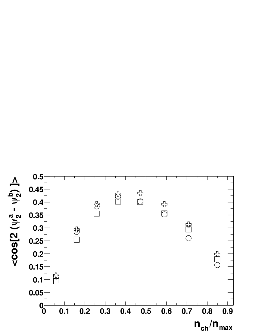
Figure 2: Correlation between the event plane angles determined from pairs of subevents partitioned randomly (circles), partitioned with opposite sign of pseudorapidity (squares) and partitioned with opposite sign of charge (crosses). The correlation is plotted as a function of centrality, namely charged particle multiplicity $n_{\rm ch}$ divided by the maximum observed charged multiplicity, $n_{\rm max}$.

Figure 2 shows the event plane correlation between two subevents, for each of three different subevent partitions. In central events, it is seen that the correlation is stronger in the case of subevents with opposite sign of charge compared to subevents partitioned randomly. This pattern might be due to resonance decays to two particles with opposite charge. The spread of the results for different subevent partitions is about 0.05, which is in accord with the number used for the estimates of the systematic errors.

The event plane resolution for full events is defined as $\langle\cos(n(\Psi_{measure}-\Psi_{true}))\rangle$, in which $\Psi_{measure}$ and $\Psi_{true}$ are azimuthal angles for the measured reaction plane and the “true” reaction plane, respectively. The resolution with $p_{t}$ weighting (see Section II.2) can reach as high as 0.8, as shown in Fig. 3. The $v_{2}$ as a function of centrality is shown in Fig. 4, using different prescriptions to partition the particles into subevents. Again, partitioning into subevents with opposite sign of charge yields the highest elliptic flow signal, presumably because of neutral resonance ($\rho^{0}$, etc.) decay.

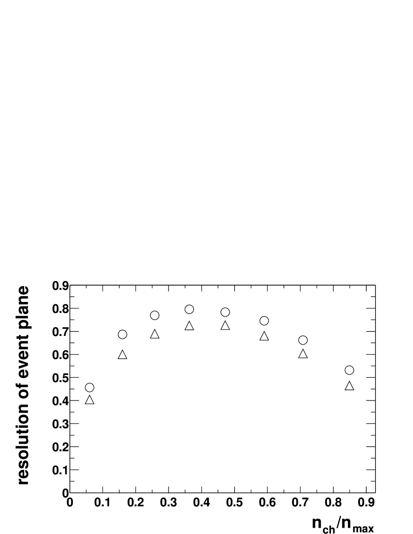
Figure 3: The event plane resolution for full events as a function of centrality, using randomly partitioned subevents with (circles) and without (triangles) $p_{t}$ weight.

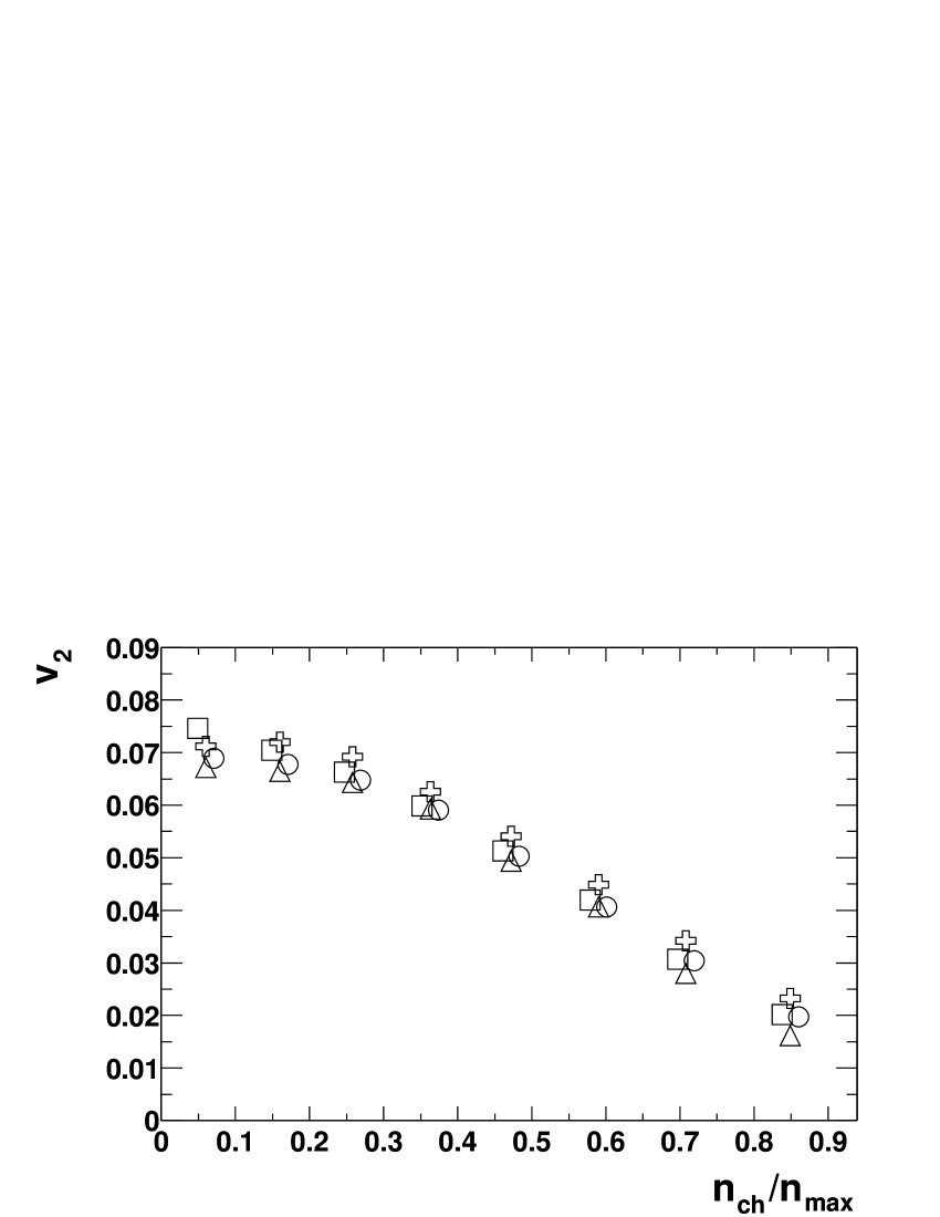
Figure 4: Elliptic flow signal $v_{2}$ as a function of centrality, from study of the correlation between particle pairs consisting of randomly chosen particles (circles), particles with opposite sign of charge (crosses), particles with the same sign of charge (triangles) and particles with opposite sign of pseudorapidity (squares).

II.2 Weighting

If Eq. (3) is generalized to the form $Q_{n}=\sum_{i}w_{i}u_{i}$, where the $w_{i}$ are weights adjusted to optimize the event plane resolution Dani95 ; Posk98 , then $u_{i}$ should be replaced by $w_{i}u_{i}$ for all equations in this paper, and $M$ should be replaced by $\sum_{i}w_{i}^{2}$ throughout Sec. II, and Sec. IV.2.

The best weight $w_{i}(\eta,p_{t})$ is $v_{2}(\eta,p_{t})$ itself Olli00 . In practice, since we know that $v_{2}$ is approximately proportional to $p_{t}$ up to about 2 GeV$/c$, it is convenient to use $p_{t}$ as the weight. It is found that $p_{t}$ weighting can reduce the statistical error significantly, as demonstrated in Fig. 5.

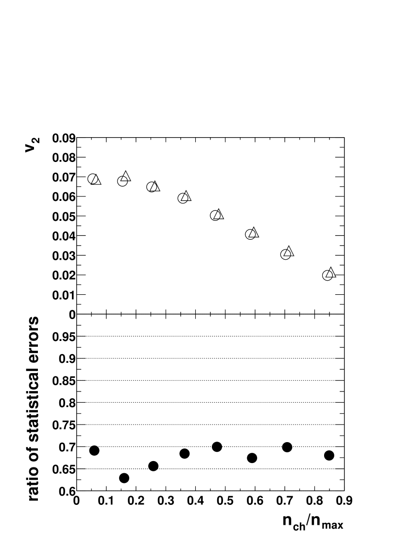
Figure 5: The upper panel shows $v_{2}$ versus centrality using the conventional method, where the circles and triangles represent $v_{2}$ with and without $p_{t}$ weighting, respectively. The statistical error is smaller than the symbol size. The lower panel shows the statistical error on $v_{2}$ with $p_{t}$ weighting divided by the same without weighting.

II.3 Scalar product flow analysis

In a new scalar product method ArtSergeiLBLReport , each event is partitioned into two subevents, labeled by the superscripts $a$ and $b$. The correlation between two subevents is

$$\langle Q^{a}_{n}{Q^{b}_{n}}^{*}\rangle=\langle v^{2}_{n}M^{a}M^{b}\rangle\,,$$ (6)

where $M^{a}$ and $M^{b}$ are the multiplicities for subevents $a$ and $b$, respectively. The vectors $Q^{a}_{n}$ and $Q^{b}_{n}$ are constructed for the appropriate subevent as per Eq. (2).

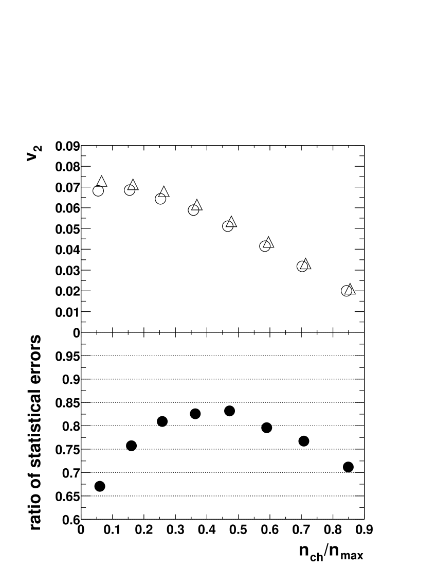
Figure 6: The upper panel presents $v_{2}$ versus centrality from the scalar product method (triangles) and the conventional random subevent method (circles). All statistical errors are smaller than the symbol size. The statistical error for the scalar product method divided by that for the conventional method is shown in the lower panel.

Given the above, the flow relative to the true reaction plane can be readily calculated from unit momentum vectors $u_{n,i}(\eta,p_{t})$ of the analyzed tracks by using Eq. (6) for the particle relative to the $2M$ other particles, and then dividing by the square root of Eq. (6) for the subevents. This gives

$$v_{n}(\eta,p_{t})=\frac{\langle Q_{n}u_{n,i}^{*}(\eta,p_{t})\rangle}{2\sqrt{\langle Q^{a}_{n}{Q^{b}_{n}}^{*}\rangle}}\,.$$ (7)

Auto-correlations are removed by subtracting particle $i$ in the calculation of $Q_{n}$ when taking the scalar product with $u_{n,i}$. This method weights events with the magnitude of the $Q_{n}$ vector, and if $Q_{n}$ is replaced by its unit vector, the above reduces to $\langle\cos n(\phi-\Psi)\rangle$, the conventional correlation method.

Figure 6 demonstrates that the results from the scalar product method are indeed very close to the ones of the conventional method. In this calculation, the subevents are generated by random partitioning. However, the detailed comparison of two results reveals a small systematic difference. The difference might have origin in the approximations (the Central Limit Theorem) used in the conventional method and that are not required in the scalar product method. In addition, the scalar product method has the benefit of smaller statistical errors and is very simple to implement.

III Distribution in the magnitude of the flow vector

In this section we study elliptic flow by analysis of the distribution in the magnitude of the flow vector. The method was used by the E877 Collaboration at the AGS for the first observation of anisotropic flow at ultra-relativistic nuclear collisions E877PRL94 . This method is based on the observation that anisotropic flow strongly modifies the distribution of the magnitude of the flow vector Volo96 ; Olli95 ; Posk98 ; Olli00 . Very strong flow leads to the distribution, $dP/(Q_{n}dQ_{n})$ with a local minimum at $Q=0$, which reflects the fact that for the case of strong flow all particle momentum unit vectors are aligned in the flow direction. On the other hand, the non-flow effects, two and few particle azimuthal correlations lead to an increase in the statistical fluctuation width of the distribution. The effect can be understood by considering the flow vector composed of many clusters but randomly distributed in the azimuthal space. In the limit of large multiplicity and neglecting the contribution from higher harmonics (for a more accurate consideration see ArtSergeiLBLReport ; Olli97 ; Olli00 ) the distribution can be described by Volo96 ; Posk98 ; Olli95 :

$$\frac{dP}{q_{n}dq_{n}}=\frac{1}{\sigma_{n}^{2}}e^{\displaystyle{-\frac{v_{n}^{2}M+q_{n}^{2}}{2\sigma_{n}^{2}}}}I_{0}(\frac{q_{n}v_{n}\sqrt{M}}{\sigma_{n}^{2}}),$$ (8)

where $I_{0}$ is the modified Bessel function. We have introduced the variable $q_{n}=Q_{n}/\sqrt{M}$, which greatly reduces the effect on the shape of the distribution from averaging over events with different multiplicities. In a more general case using weights, one should use $q_{n}=Q_{n}/(\sqrt{M\langle w_{i}^{2}\rangle}$). In this way the width of the $q-$distribution is independent of multiplicity:

$$\sigma_{n}^{2}=0.5(1+g_{n}),$$ (9)

with $g_{n}$ reflecting the change in the width of the distribution due to non-flow effects (and to some extent to the averaging over events with different multiplicities).

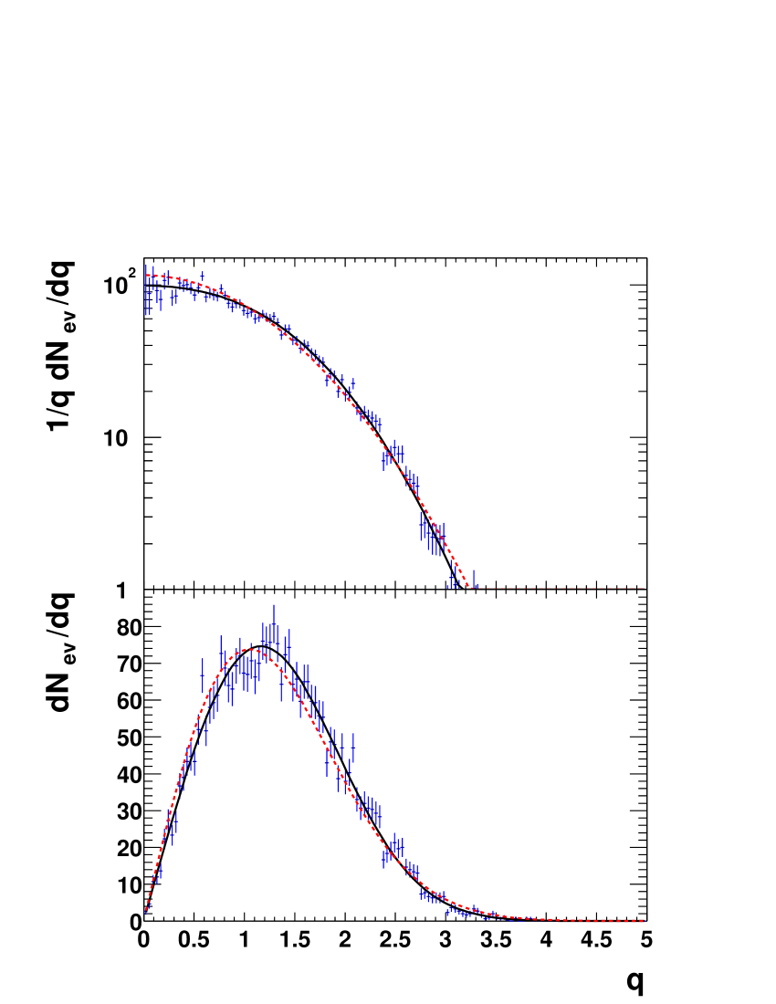
Figure 7: Reduced flow vector distributions for centrality bin 5 plotted in two ways. Solid lines correspond to the fit with two parameters, $v_{2}$ and $g_{2}$, and dashed lines correspond to the fit assuming zero real flow.

We have fitted distributions of $q_{2}$, the second harmonic reduced flow vector, in two different ways. First, the distributions in all different centrality bins have been fitted with two independent parameters, $v_{2}$ and $g_{2}$. The non-flow contribution parameter, $g_{2}$, has been found to be in the range of 0.18 –0.32 for all centralities except the most peripheral one. One should not expect a good fit for the most peripheral bin, for it is a mixture of events in a wide multiplicity range from 20 to 100. Better fit results for this bin could be achieved if the bin would be split into several sub-bins with smaller relative multiplicity variations. The relative multiplicity variation in the other bins is much smaller. The $q$ distribution for the centrality bin 5 is presented in Fig. 7. The two fit functions correspond to the case of a fit with two parameters, $v_{2}$ and $g_{2}$, and to the case of a one parameter fit of $g_{2}$ for $v_{2}=0$. Note that the dashed curves are systematically higher or lower than the data points in different $q$ regions. In the lower part of Fig. 7 one can see that the anisotropic flow pushes the q distribution out to larger values. If the flow were great enough one could select events based on the q values.

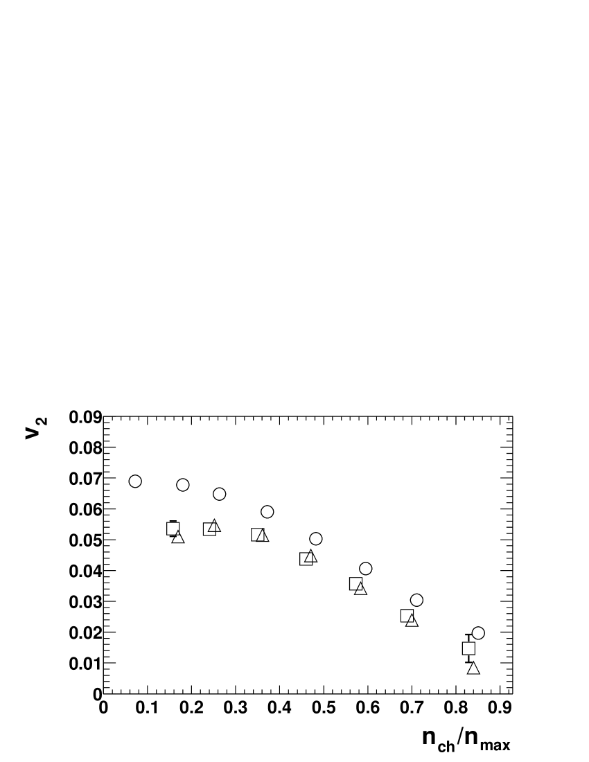
Figure 8: Elliptic flow as determined from the fits to the $q$ distributions in different centrality bins. The circles are from the standard method with random subevents. For the squares, all the centralities were fit separately. For the triangles, centrality bins 2 to 8 were fit with the same value of the non-flow parameter.

In the second method we fit $q$ distributions in centrality bins 2 to 8 simultaneously with different $v_{2}$ values for each centrality bin but the same value of $g$. (This assumption is similar to the assumption of $\tilde{\delta}=const$ in the previous section. See also the discussion in Olli95 ; Posk98 ; Olli00 ). We find $g=0.29\pm 0.02$. The results of the fits are presented in Fig. 8. The deviation from the standard method results are due to the non-flow contributions.

IV Four-particle correlations

IV.1 Motivation for Cumulants

In experiments, it is necessary to rely on correlations between particles to determine the event plane since the reaction plane is not a direct observable. The assumption underlying conventional pair correlation analyses (including the scalar product method discussed in section II.C above) is that non-flow correlations of the type mentioned in section I are negligible compared to the flow, or at most, are comparable to other systematic uncertainties. In past studies Posk98 ; Mai ; borghiniNoflow , non-flow correlations have been discussed with specific reference to their origin, such as momentum conservation, Bose-Einstein correlations, Coulomb effect, jets, resonance decays, etc. In the first two studies of elliptic flow in STAR STAR01 ; STAR01b , the non-flow effect from jets and resonances was estimated using the approach explained in section II.A above, and this established an upper limit on the non-flow contribution to the reported $v_{2}$ signal. This limit played a role in determining the systematic error on the published measurements.

Anisotropic flow is a genuine multiparticle phenomenon, which justifies use of the term collective flow. It means that if one considers many-particle correlations instead of just two-particle correlations, the relative contribution of non-flow effects (due to few particle clusters) should decrease. Considering many-particle correlations, one has to subtract the contribution from correlations due to lower-order multiplets. Formally, one should use cumulants Biya81 ; Libo89 ; Egge93 ; Olli01 instead of simple correlation functions. Let us explain this with an example for four-particle correlations. The correlation between two particles is

$$\langle u_{n,1}u_{n,2}^{*}\rangle\equiv\langle e^{in\phi_{1}}e^{-in\phi_{2}}\rangle=v_{n}^{2}+\delta_{n}\,,$$ (10)

where $n$ is the harmonic, and the average is taken over all pairs of particles in a given rapidity and transverse momentum region, and over all events in an event sample. The $\delta_{n}$ represents the contribution to the pair correlation from non-flow effects. Correlating four particles, one gets

$$\langle u_{n,1}u_{n,2}u_{n,3}^{*}u_{n,4}^{*}\rangle=v_{n}^{4}+2\cdot 2\cdot v_{n}^{2}\delta_{n}+2\delta_{n}^{2}\,.$$ (11)

In this expression, two factors of “2” in front of the middle term correspond to the two ways of pairing (1,3)(2,4) and (1,4)(2,3) and account for the possibility to have non-flow effects in the first pair and flow correlations in the second pair and vice versa. The factor “2” in front of the last term is due to the two ways of pairing. The pure four-particle non-flow correlation is omitted from this expression — see the discussion below about the possible magnitude of such a contribution. What is remarkable is that if one subtracts from the expression (11) twice the square of the expression (10), one is left with only the flow contributions

$$\langle\langle u_{n,1}u_{n,2}u_{n,3}^{*}u_{n,4}^{*}\rangle\rangle$$

$$\equiv\langle u_{n,1}u_{n,2}u_{n,3}^{*}u_{n,4}^{*}\rangle-2\langle u_{n,1}u_{n,2}^{*}\rangle^{2}=-v_{n}^{4}\,,$$ (12)

where the notation $\langle\langle...\rangle\rangle$ is used for the cumulant. The cumulant of order two is just $\langle\langle u_{n,1}u_{n,2}^{*}\rangle\rangle=\langle u_{n,1}u_{n,2}^{*}\rangle$.

In flow analysis, one is interested not only in so-called “global” flow values, but also in differential flow as function of rapidity and transverse momentum. In a four-particle correlation approach, this also can be done in a similar manner, now correlating a particle, for example in a particular $p_{t}$ bin, with three particles from a common “pool”. Assuming that the particle “b” is the one from a particular bin, one gets for a differential flow study

$$\langle u_{n,b}u_{n,1}^{*}\rangle=v_{n;b}v_{n}+\delta_{n;b}\,,$$ (13)

where we have introduced the notation $v_{n;b}$ for the flow value corresponding to the bin under study, and $\delta_{n;b}$ for the corresponding non-flow contribution. Then for the correlation with three particles from the pool,

$$\langle u_{n,b}u_{n,1}u_{n,2}^{*}u_{n,3}^{*}\rangle=$$

$$v_{n;b}v_{n}^{3}+2\cdot v_{n}^{2}\delta_{n;b}+2\cdot v_{n}v_{n;b}\delta_{n}+2\delta_{n}\delta_{n;b}\,.$$ (14)

In this case, in order to remove the non-flow contribution, one has to subtract from (14) twice the product of expressions (10) and (13).

$$\langle u_{n,b}u_{n,1}u_{n,2}^{*}u_{n,3}^{*}\rangle-2\langle u_{n,b}u_{n,1}^{*}\rangle\langle u_{n,1}u_{n,2}^{*}\rangle=$$ (15)

$$-v_{n}^{3}v_{n;b}\,.$$

Assuming that the average flow value for the particles in the pool is known, one gets the desired differential flow value for the particular bin under study.

In Eq. (11), we have neglected the contribution from the pure four-particle correlations due to non-flow effects. Let us now estimate the upper limit for such a contribution. Assume that all particles are produced via four-particle clusters. All daughters of the decay of such a cluster could in principle be within 1–2 units of rapidity from each other. Then the contribution would be

$$6f/M^{3},$$ (16)

where $M$ is the total multiplicity within those 1–2 units of rapidity, and $f$ is $\langle(\cos 2(\phi_{1}-\phi_{2}))^{2}\rangle$ averaged over all cluster decay products. Assuming a perfect alignment, $f=1$, and multiplicity $M=1000$, this would give us a possible error in $v_{2}$ measurements of the order of

$$\delta v\sim(v_{2}^{4}+6/1000^{3})^{1/4}-v_{2}\,.$$ (17)

This would give only 3% relative error on $v_{2}$ signal of 0.015, and would drops very rapidly with increasing real $v_{2}$ signal. This calculation is for the case of 100% of the particle production via four-particle clusters and a perfect alignment of decay products. A more realistic scenario would give a much smaller estimate.

IV.2 Four-subevent method

In order to apply the four-particle correlation approach to the analysis of real data, one should perform an average over all possible quadruplets of particles in a given event. Bearing in mind that the average multiplicity in a central STAR event is well beyond a thousand, it becomes a nontrivial task. The simplest solution to the problem is the four-subevent method where one partitions all tracks (for example, randomly) into four groups (subevents) and calculates a flow vector for each of the groups,

$$Q_{n}=\sum_{i}u_{n,i}\,,$$ (18)

where the sum is over all particles in the group. Using these subevents, the problem becomes much simpler computationally. For example,

$$\langle u_{n,1}u_{n,2}u_{n,3}^{*}u_{n,4}^{*}\rangle=\langle Q_{n,1}Q_{n,2}Q_{n,3}^{*}Q_{n,4}^{*}/(M_{1}M_{2}M_{3}M_{4})\rangle\,,$$ (19)

where $M_{i}$ are the corresponding subevent multiplicities. The cumulant calculation is straightforward:

$$\langle\langle u_{n,1}u_{n,2}u_{n,3}^{*}u_{n,4}^{*}\rangle\rangle=$$

$$\langle\frac{Q_{n,1}Q_{n,2}Q_{n,3}^{*}Q_{n,4}^{*}}{M_{1}M_{2}M_{3}M_{4}}\rangle$$

$$-2\left(\langle Q_{n,1}Q_{n,2}^{*}/(M_{1}M_{2})\rangle\right)^{2}.$$ (20)

The four-subevent method is very simple, both in logic and in implementation. The price for these benefits is lower statistical power, because the method does not take into account all possible quadruplets. Some improvement could be reached by splitting the event into more than four subevents and correlating all possible combinations of four. In the analysis of the STAR data we use eight subevents. A more general cumulant formalism, based on the cumulant generating function Mai ; Olli01 offers advantages for a four-particle analysis in the context of the present limited sample size.

IV.3 Cumulant generating function

The cumulant and generating function approach offers a formal and convenient way to study flow and non-flow contributions systematically. Following the method of Ref. Olli01 , the cumulant to order four is defined by

$$\langle\langle u_{1}u_{2}u_{3}^{*}u_{4}^{*}\rangle\rangle\equiv\langle u_{1}u_{2}u_{3}^{*}u_{4}^{*}\rangle-$$

$$\langle u_{1}u_{3}^{*}\rangle\langle u_{2}u_{4}^{*}\rangle-\langle u_{1}u_{4}^{*}\rangle\langle u_{2}u_{3}^{*}\rangle\,,$$ (21)

where, as above, the double angle bracket notation represents the cumulant expression shown explicitly on the right-hand side. The subscript for the harmonic order, $n$, has been dropped. The cumulant $\langle\langle u_{1}u_{2}u_{3}^{*}u_{4}^{*}\rangle\rangle$ involves only pure four-particle correlations, since the two-particle only correlations among the quadruplets have been explicitly subtracted away.

In the presence of flow, the cumulant becomes

$$\langle\langle u_{1}u_{2}u_{3}^{*}u_{4}^{*}\rangle\rangle=-v^{4}_{n}+O(\frac{1}{M^{3}}+\frac{v^{2}_{2n}}{M^{2}})\,,$$ (22)

where $M$ is the multiplicity of the events, the term of order $1/M^{3}$ represents the remaining four-particle non-flow effects, and the term of order $v^{2}_{2n}/M^{2}$ is the contribution of the $2n$ higher harmonic. The cumulant to higher orders and the corresponding generalization has also been determined Olli01 . Likewise, the cumulant of order two reduces to the equivalent of a pair correlation analysis of the conventional type. Statistical uncertainties associated with a cumulant analysis increase with increasing order from 2 to 4.

The definition of the cumulant is simple, but it is tedious to calculate the moments term-by-term on the right-hand side of Eq. (21). Fortunately, the cumulant can be computed more easily from the generating function Olli01 ,

$$G_{n}(z)=\prod_{j=1}^{M}\left(1+{z^{*}u_{j}+zu_{j}^{*}\over M}\right),$$ (23)

where $z\equiv|z|e^{i\alpha}$ is an arbitrary complex number, $z^{*}$ denotes its complex conjugate. The generating function itself has no direct physical meaning, but the coefficients of the expansion of $\langle G_{n}\rangle$ in powers of $z,z^{*}$ yield the correlations of interest:

$$\langle G_{n}\rangle = 1+\langle\frac{M-1}{M}\rangle|z|^{2}\langle u_{1}u_{2}^{*}\rangle$$

$$+ \langle\frac{(M-1)(M-2)(M-3)}{4M^{3}}\rangle|z|^{4}\langle u_{1}u_{2}u_{3}^{*}u_{4}^{*}\rangle+....$$

One can use these correlations to construct the cumulants. In the limit of large $M$, $\langle G_{n}\rangle$ can be used to obtain the cumulant generating function directly:

$$M\cdot\left(\langle G_{n}(z)\rangle^{1/M}-1\right)=$$

$$\sum_{k}{|z|^{2k}\over(k!)^{2}}\langle\langle u_{1}...u_{k}u_{k+1}^{*}...u_{2k}^{*}\rangle\rangle\,.$$ (25)

The left-hand side of Eq. (25) is what is measured, and in order to extract the cumulants on the right, $k$ equations of the form of Eq. (25) are needed to solve for $k$ undetermined parameters. This can be accomplished by repeating the process with $k$ different values of $|z|$. It is found that suggested magnitudes of $|z|$ in Ref. Olli01 , namely $r_{0}\sqrt{p}$ with $r_{0}=1.5$ and $p=1,\cdots k$, are fairly good, since results from optimized values cumuPraticeGuide of $r_{0}$ show almost no difference. Results in this paper are by default calculated with $r_{0}=1.5$. Since $M$ fluctuates from one event to the other, for events within a multiplicity bin, we use the average value $\langle M\rangle$ in Eq. 25 instead of $M$.

For experimental analysis, it is sufficient to take the first three terms in Eq. (25). Once the cumulant has been computed, extracting the integrated flow value is straightforward because, for instance, $v^{4}_{n}=-\langle\langle u_{1}u_{2}u_{3}^{*}u_{4}^{*}\rangle\rangle$.

When a non-unit weight is used, the integrated flow value described above becomes $\langle w\cos n\phi^{\prime}\rangle$, which is not exactly $v_{n}$ but an approximation. However, the differential flow can be calculated exactly (see below) no matter what weight is used. The integrated flow with non-unit weight can be obtained by integrating the differential flow. All integrated flow results in this paper (except for results from the four-subevent method) are obtained by integrating over the differential flow.

For differential flow (flow in a bin of $\eta$ and/or $p_{t}$), Eq. (25) is replaced by

$$\frac{\langle u_{d}G_{n}(z)\rangle}{\langle G_{n}(z)\rangle}\equiv$$

$$\sum_{k,l}{z^{*k}z^{l}\over k!\,l!}\langle\langle u_{d}u_{1}...u_{k}u_{k+1}^{*}...u_{k+l}^{*}\rangle\rangle\,.$$ (26)

where $u_{d}$ is the unit vector for a particle in the selected bin. Following a similar procedure as in the case of the integrated flow, the cumulant $\langle\langle u_{d}u_{1}u_{2}^{*}u_{3}^{*}\rangle\rangle$ is computed, but it now contains the angle of the one particle of interest and three other particles from the pool. Then the differential flow is Olli01

$$v_{n}=-\frac{\langle\langle u_{d}u_{1}u_{2}^{*}u_{3}^{*}\rangle\rangle}{(-\langle\langle u_{1}u_{2}u_{3}^{*}u_{4}^{*}\rangle\rangle\,)^{3/4}}.$$ (27)

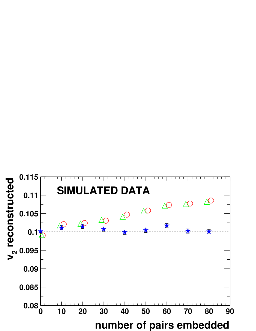
Figure 9: Reconstructed $v_{2}$ from the conventional method (circles), from the 2nd-order cumulant method (triangles), and from the 4th-order cumulant method (stars), for simulated events as a function of number of embedded back-to-back track pairs. The horizontal dashed line marks the level of the true elliptic flow $v_{2}=0.10$, as imposed on the simulated events, including the back-to-back track pairs. The statistical error is smaller than the symbol size. The multiplicity for all events is 500.

Eq. (27) is for unit weight. It can be easily generalized for non-unit weight, and the formula still holds.

Some detectors have substantial asymmetry in their response as a function of azimuth in detector coordinates, in which case it is necessary to prevent distortion of the measured flow signals by employing one of two possible compensation methods Posk98 — applying a shifting transformation which recenters $Q$: $\langle Q_{n}\sin n\Psi_{n}\rangle=0$ and $\langle Q_{n}\cos n\Psi_{n}\rangle=0$ (see Eq. ( 2)), or applying weighting factors to force a flat $\Psi$ distribution. In the present study, no noticeable difference is observed with and without explicit compensation for detector asymmetry, as expected in light of the excellent azimuthal symmetry of the STAR TPC. All plots in this paper are made without compensation for detector asymmetry. However, it should be noted that cumulants, as defined by the generating function, also correct for small anisotropies in the detector acceptance. For instance, the cumulant

$$\langle\langle u_{1}u_{2}^{*}\rangle\rangle=\langle u_{1}u_{2}^{*}\rangle-\langle u_{1}\rangle\langle u_{2}^{*}\rangle$$ (28)

amounts to an implementation of the shifting compensation method mentioned above.

IV.4 Simulations

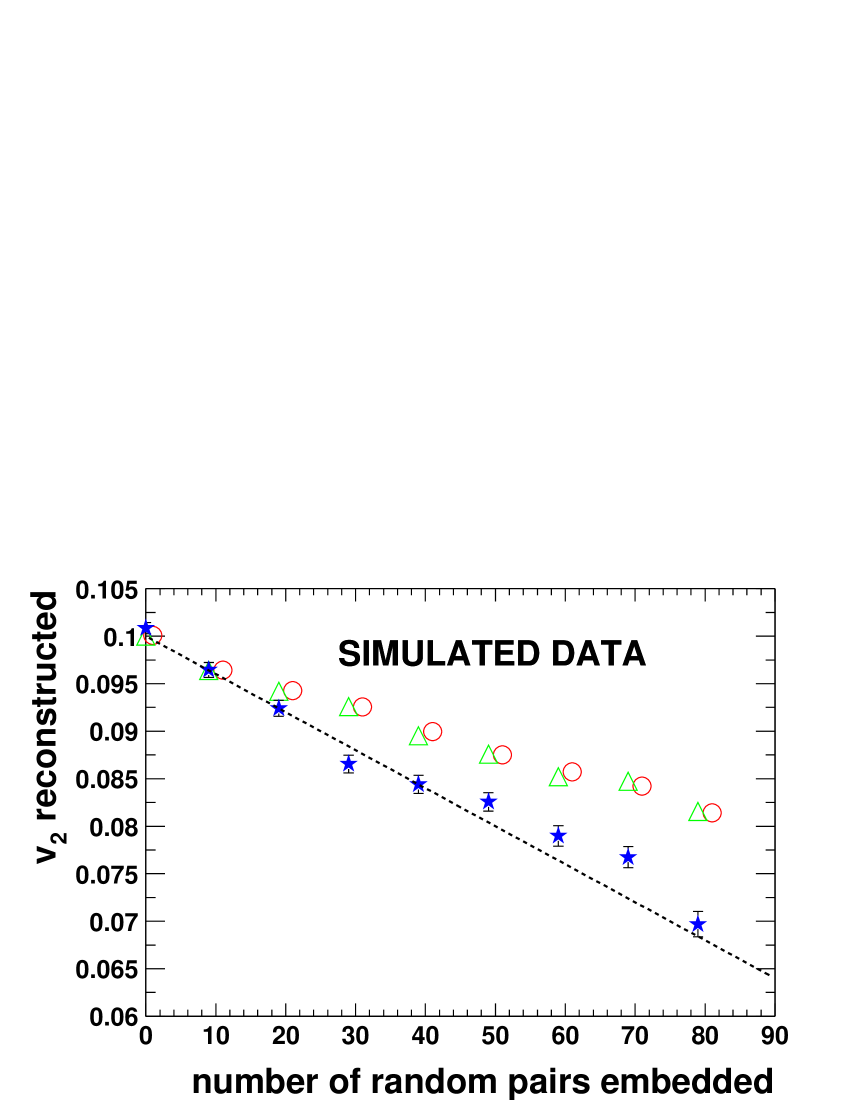
Figure 10: Reconstructed $v_{2}$ from the conventional method (circles), from the 2nd-order cumulant method (triangles), and from the 4th-order cumulant method (stars), for simulated events as a function of number of embedded back-to-back track pairs. Unlike in the previous figure, the embedded back-to-back pairs are randomly distributed relative to the event plane, and so the true resultant $v_{2}$, indicated by the dashed line, decreases as more pairs are embedded. The multiplicity for all events is 500.

In order to test the cumulant method as well as the analysis procedure, the MEVSIM mevsim event generator has been used to make events with various mixtures of flow and non-flow effects. In all cases, the number of simulated events in a data set is 20k, and the multiplicity is 500. Fig. 9 shows one such set of simulations. Nine data sets with $v_{2}=0.10$ were produced, then a simple non-flow effect consisting of embedded back-to-back track pairs was introduced at various levels, ranging from zero up to 80 pairs per simulated event. These pairs simulate resonances which decay to two daughters with a large energy release. In Fig. 9, we consider the scenario where the embedded pairs themselves are correlated with the event plane with the same $v_{2}=0.10$. Fig. 9 shows that the 4th-order cumulant $v_{2}$ always reconstructs the expected 10% $v_{2}$, while the $v_{2}$ from the pair correlation analysis methods can only recover the correct input if non-flow pairs are not embedded.

If back-to-back pairs are instead randomly distributed in azimuth, the true flow should decreases and the expected variation can be computed knowing the number of random tracks. Fig. 10 shows such a simulation, and again it is found that only the 4th-order cumulant $v_{2}$ agrees with the expected elliptic flow, while the inferred $v_{2}$ based on pair correlation analyses is distorted in the presence of the simulated non-flow effects. The role of resonances produced in real collisions may be closer to one or the other of the above two simulated scenarios, but in either case, the non-flow effect is removed by the 4th-order cumulant analysis.

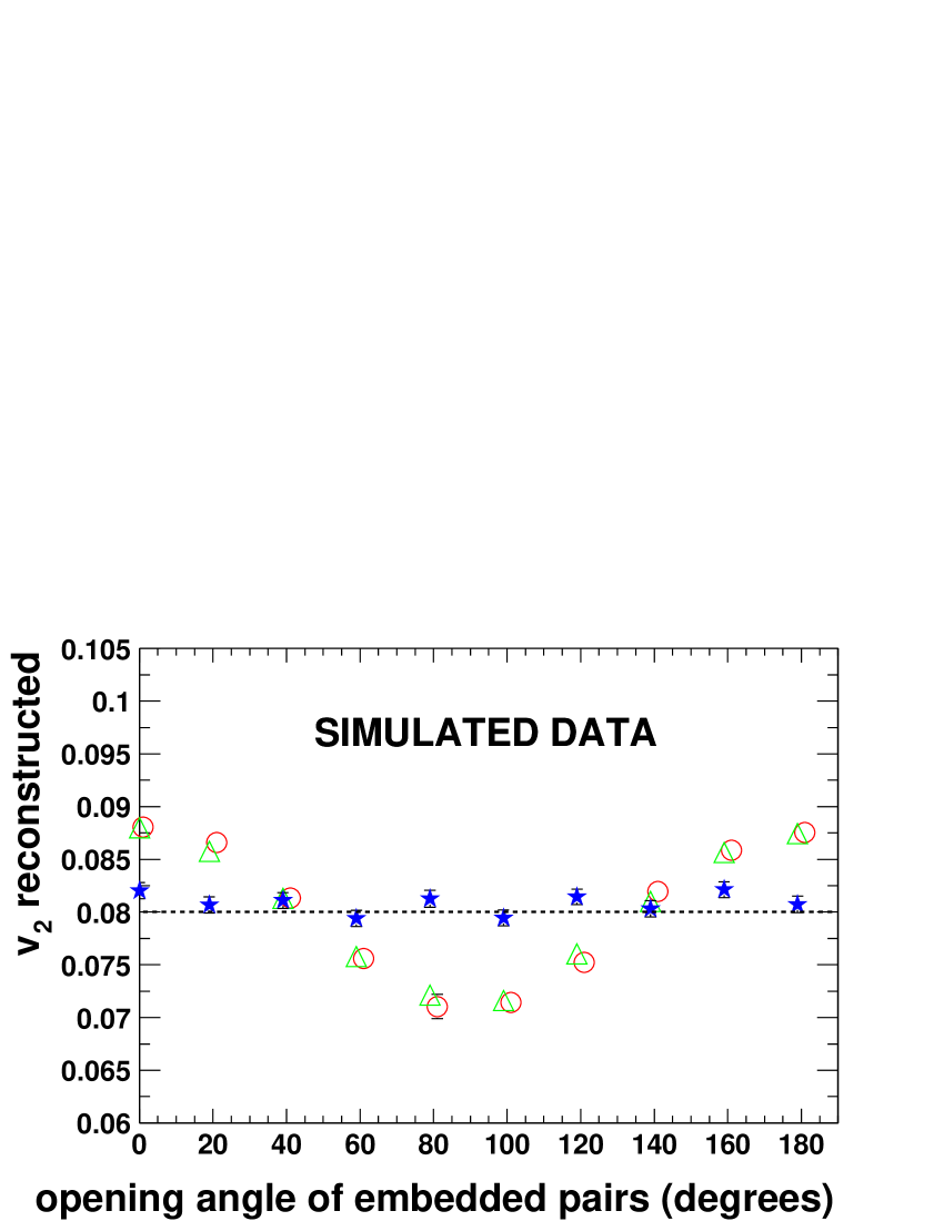
Figure 11: Elliptic flow from the conventional method (circles), from the 2nd-order cumulant method (triangles), and from the 4th-order cumulant method (stars), for simulated events as a function of azimuthal angle between the two tracks in each of 50 embedded pairs per event, with the 50 pairs each having random orientation relative to the event plane. The horizontal dashed line marks the level of the true elliptic flow $v_{2}$ = 0.08.

In Fig. 11, consideration is given to the possible effect of resonances which decay with smaller energy release, having an azimuthal opening angle $\Phi$ in the laboratory. The simulated events were generated with an imposed flow $v_{2}=0.08$, while in each event 50 pairs with the same $\Phi$ were embedded, each such pair having a random orientation relative to the event plane. Ten data sets were produced, with $\Phi$ (the abscissa in Fig. 11) varying in $20^{\circ}$ steps between zero and $180^{\circ}$. Again, only the 4th-order cumulant $v_{2}$ (stars) recovers the true elliptic flow signal.

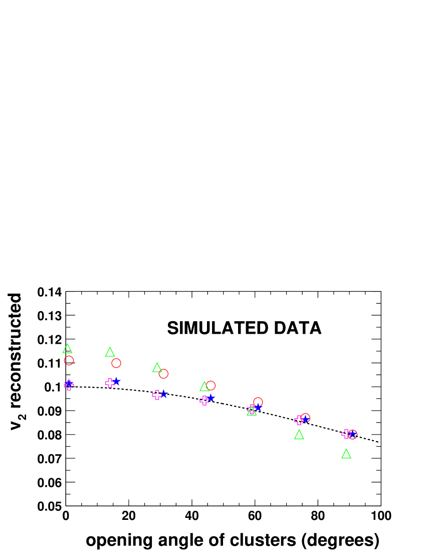
Figure 12: Elliptic flow from the conventional method (circles), and from the 2nd-order (triangles), 4th-order (stars), and 6th-order (crosses) cumulant methods. This is for simulated events as a function of azimuthal angle between two back-to-back track pairs. The dashed line marks the level of the true elliptic flow.

In order to test how the various methods respond to non-flow correlations associated with four-particle clusters, the simulated events in Fig. 12 were generated with an imposed flow $v_{2}=0.10$, after which 25 four-particle clusters were embedded in each event. Each cluster consists of two back-to-back pairs with an azimuthal opening angle $\Phi$ between them. Seven data sets were produced, with $\Phi$ (the abscissa in Fig. 12) varying in $15^{\circ}$ steps between zero and $90^{\circ}$. The clusters were oriented such that a track bisecting $\Phi$ would contribute to the overall flow with $v_{2}=0.10$. The 4th-order cumulant (stars) and the 6th-order cumulant (crosses) both reconstruct the true elliptic flow (dotted line). Note that the four-particle correlation introduced by the clusters is $~{}1/M^{2}$ times the pair correlation part, resulting in little difference between $v_{2}$ from the 4th- and 6th-order cumulant methods. This result further illustrates the point (see also the end of section III.A) that non-flow effects are believed to contribute at a negligible level to the four-particle correlation, and for this reason, there may be little advantage in extending cumulant analyses to orders higher than 4.

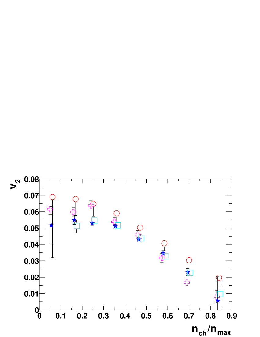
Figure 13: Measured elliptic flow versus centrality for Au + Au at $\sqrt{s_{NN}}=130$ GeV. The circles show the conventional $v_{2}$ with estimated systematic uncertainty due to non-flow QM2001Raimond , the stars show the 4th-order cumulant $v_{2}$ from the generating function, the crosses show the conventional $v_{2}$ from quarter-events, and the squares show the 4th-order cumulant $v_{2}$ from the four-subevent method.

IV.5 Results from STAR

Figure 13 shows measured elliptic flow versus centrality, where the latter is characterized by charged particle multiplicity $n_{\rm ch}$ divided by the maximum observed charged particle multiplicity, $n_{\rm max}$. The conventional $v_{2}$ (circles), the 4th-order cumulant $v_{2}$ from the generating function (stars), and the 4th-order cumulant $v_{2}$ from the four-subevent method (squares) are compared. The cross symbols in Fig. 13 represent the conventional $v_{2}$ signal for the case where each observed event is partitioned into four quarter-events, which are then analyzed like independent events. All tracks in each quarter-event have the same sign of charge, and the same sign of pseudorapidity. Furthermore, the event plane for quarter-events is constructed using only tracks with $p_{t}<0.5$ GeV$/c$, which serves to minimize the influence of non-flow associated with high-$p_{t}$ particles. It is clear that the non-flow effect is present at all centralities, and its relative magnitude is least at intermediate multiplicities.

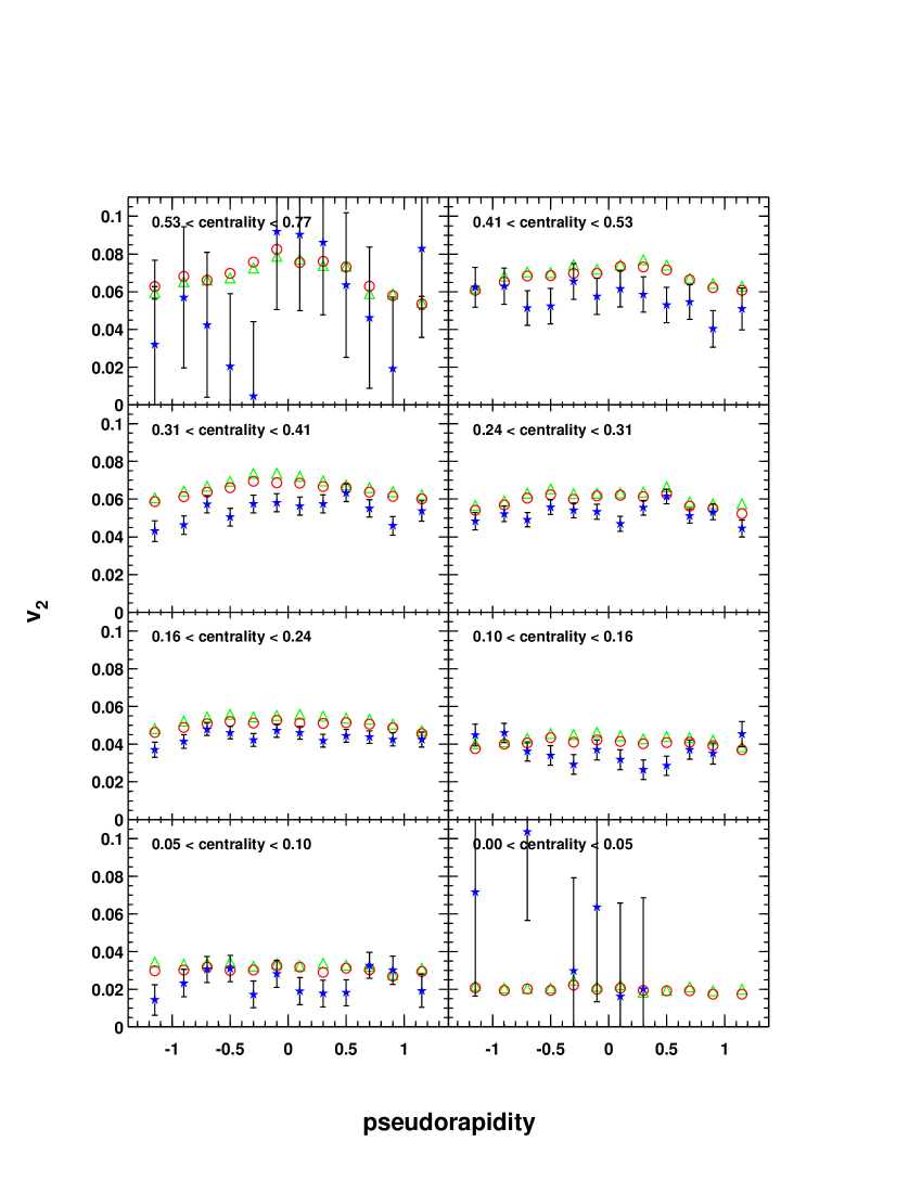
Figure 14: Reconstructed $v_{2}$ versus pseudorapidity from the conventional method (circles), from the 2nd-order cumulant method (triangles), and from the 4th-order cumulant method (stars), in eight centrality bins. The upper left panel shows the most peripheral events, and the lower right the most central.

Figure 14 shows $v_{2}$ as a function of pseudorapidity and Fig. 15 shows $v_{2}$ as a function of transverse momentum. The eight panels correspond to the eight bins of relative multiplicity in Fig. 13 but the centrality is now defined in terms of the total geometric cross section (see first three columns of table 1). These results illustrate the main disadvantage of the higher-order cumulant approach compared with any of the two-particle methods, namely, larger statistical errors, and this can be seen to be a serious shortcoming in cases where simultaneous binning in several variables results in small sample sizes. However, Fig. 13 demonstrates that, especially for the more peripheral bins, the statistical uncertainties for the fourth-order cumulant method are smaller than the systematic uncertainties for the two-particle methods.

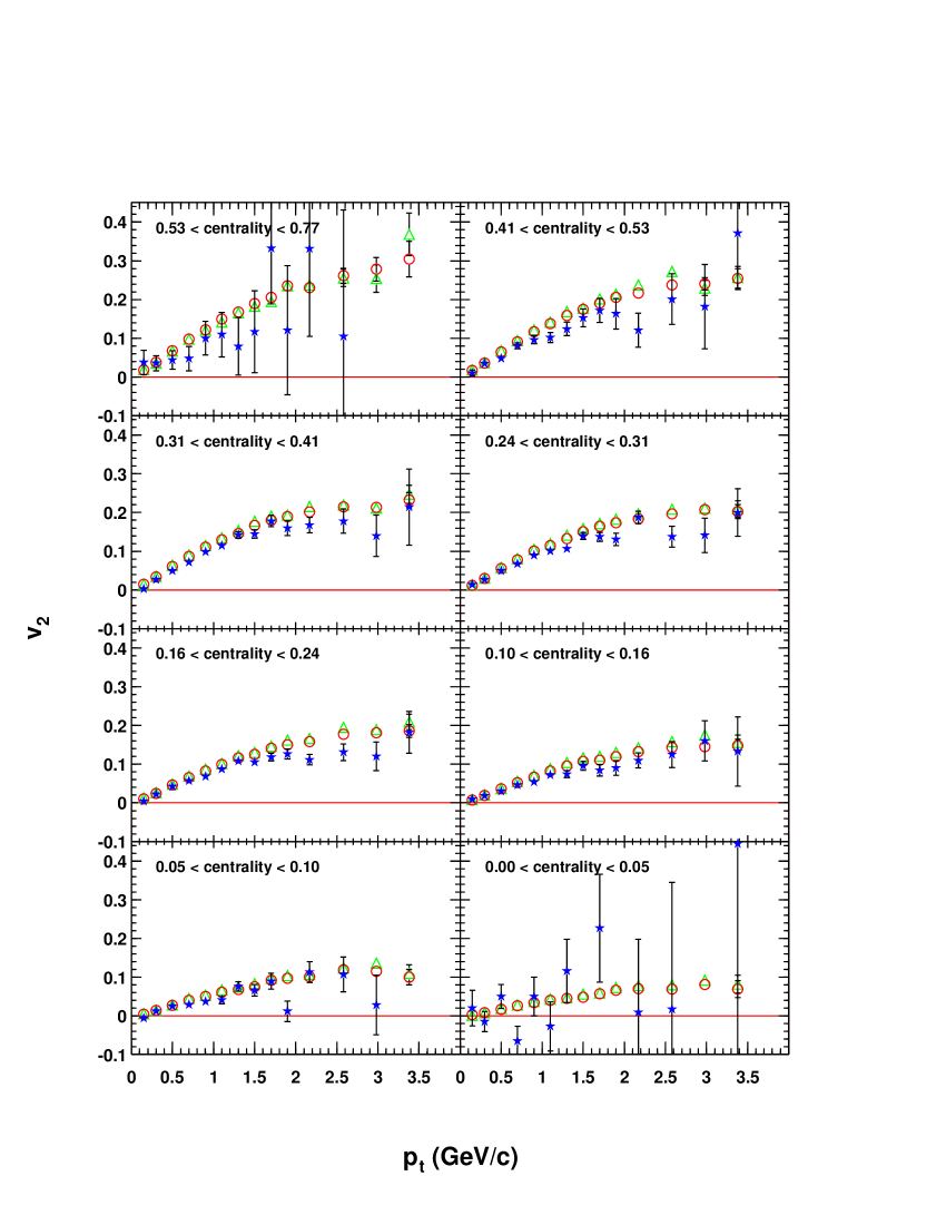
Figure 15: Reconstructed $v_{2}$ versus $p_{t}$ from the conventional method (circles), from the 2nd-order cumulant method (triangles), and from the 4th-order cumulant method (stars), in eight centrality bins. The upper left panel shows the most peripheral events, and the lower right the most central.

Figures 16 and 17 are again plots of elliptic flow versus pseudorapidity and versus transverse momentum, respectively. Here the $v_{2}$ is integrated over centrality bins 2 through 7. Bins 1 and 8 are not included in this average, otherwise they would significantly increase the statistical error on the result. The 4th-order cumulant $v_{2}$ is systematically about 15% lower than the conventional pair and cumulant pair calculations, indicating that non-flow effects contribute to $v_{2}$ analyses of the latter kind. The $v_{2}$ signal based on quarter-events (as defined in the discussion of Fig. 13) is closer to the 4th-order cumulant, although still larger on average, implying that this pair analysis prescription is effective in removing some, but not all, non-flow effects.

Figure 17 verifies that the $v_{2}(p_{t})$ curve flattens above 2 GeV/$c$ QM2001Raimond . There is theoretical interest in the question of whether or not $v_{2}(p_{t})$ continues flat at higher $p_{t}$ or eventually goes down GVW01 — this issue is the subject of a separate analysis STARnew , and the statistics of year-one data from STAR is not suited for addressing this question via a four-particle cumulant analysis.

Figure 18 presents the $p_{t}$-dependence of the correction factor for non-flow. Within errors, the relative non-flow effect is seen to be about the same or increasing very weakly from low $p_{t}$ through $p_{t}\sim 4$ GeV$/c$ — a somewhat surprising result, given the presumption that the processes responsible for non-flow are different at low and high $p_{t}$. Fig. 19, which presents $v_{2}$ from quarter-events divided by the conventional $v_{2}$, both based on event planes constructed from particles with $p_{t}<0.5$ GeV$/c$, offers a useful insight regarding the approximate $p_{t}$-independence of non-flow. This ratio roughly characterizes the contribution to non-flow from resonance decays and from other sources which primarily affect $v_{2}$ at lower $p_{t}$, whereas non-flow from (mini)jets ought to be about equally present in the numerator and the denominator of the ordinate in Fig. 19. A comparison of Figs. 18 and 19 accordingly does not contradict the implicit assumption that different phenomena dominate non-flow in different $p_{t}$ regions, and implies that the total resultant non-flow correction by coincidence happens to be roughly the same throughout the $p_{t}$ range under study.

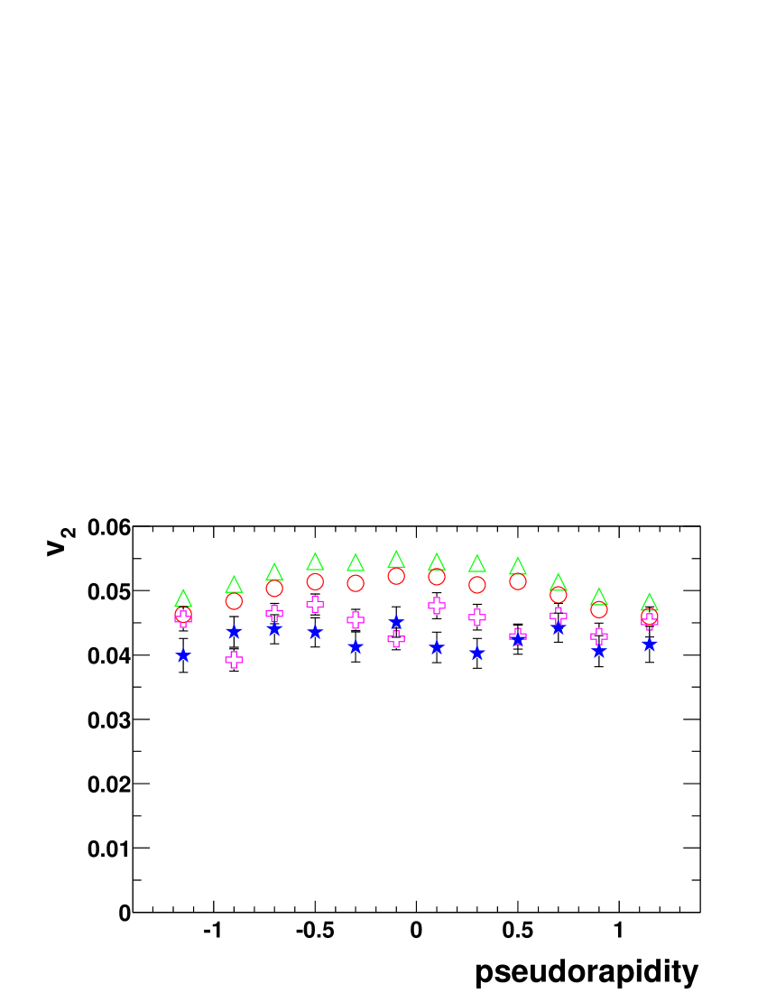
Figure 16: Elliptic flow versus pseudorapidity from the conventional method (circles), from the 2nd-order cumulant method (triangles), from quarter-events (crosses), and from the 4th-order cumulant method (stars), averaged over all centralities from bin 2 through 7, as defined in Figs. 14 and 15.

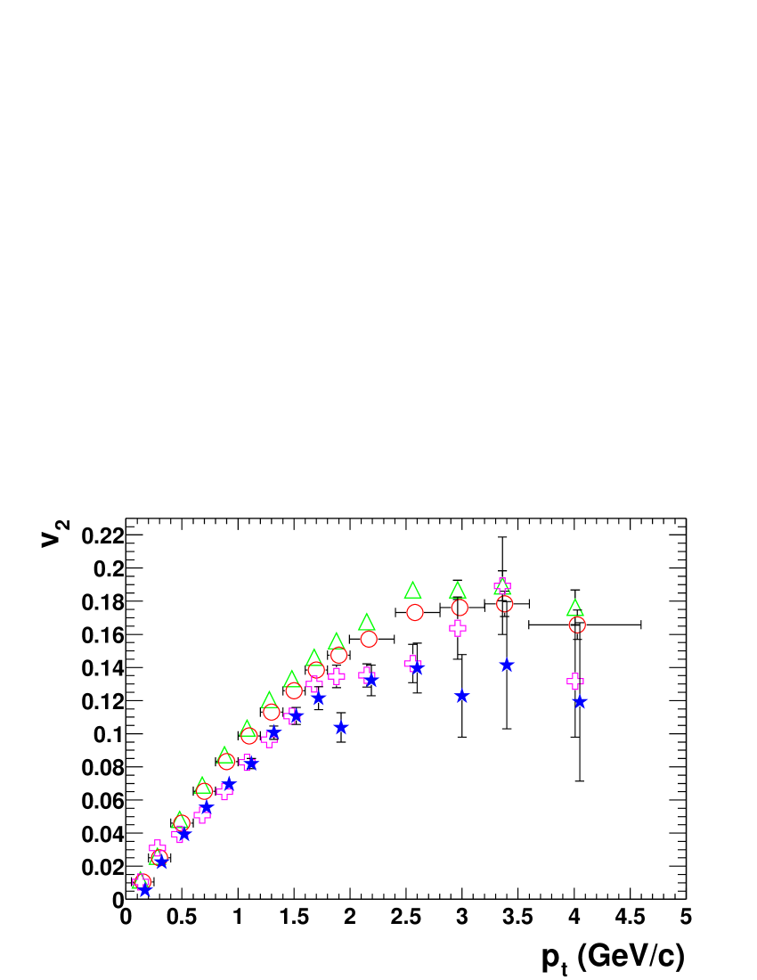
Figure 17: Elliptic flow versus transverse momentum from the conventional method (circles), from the 2nd-order cumulant method (triangles), from quarter-events (crosses), and from the 4th-order cumulant method (stars), averaged over all centralities from bin 2 through 7, as defined in Figs. 14 and 15.

Following the approach of Section II.B, the options of weighting each track by either unity or $p_{t}$ have been compared in the 4th-order cumulant analysis. Fig. 20 demonstrates that the STAR results are consistent in the two cases, and the $p_{t}$ weighting yields smaller statistical errors. All STAR results presented in this paper are computed with $p_{t}$ weighting unless otherwise stated.

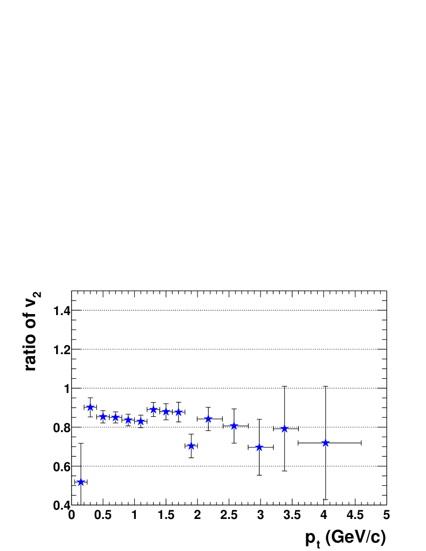
Figure 18: The ratio of $v_{2}$ from the 4th-order cumulant divided by $v_{2}$ from the conventional method as a function of $p_{t}$, averaged over all centralities from bin 2 through 7, as defined in Figs. 14 and 15.

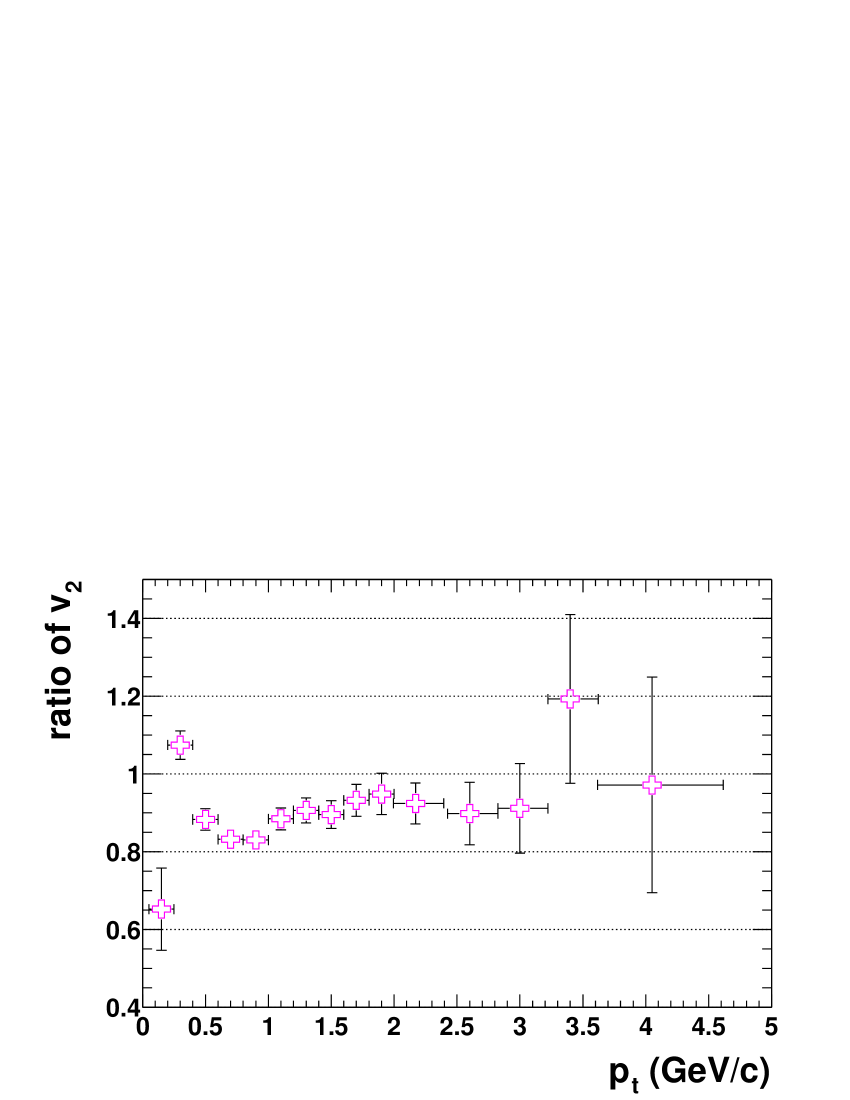
Figure 19: The ratio of $v_{2}$ from quarter-events divided by the conventional $v_{2}$ as a function of $p_{t}$. In both cases, event planes were constructed from low $p_{t}$ ($<0.5$ GeV/c) particles. The data are averaged over all centralities from bin 2 through 7, as defined in Figs. 14 and 15.

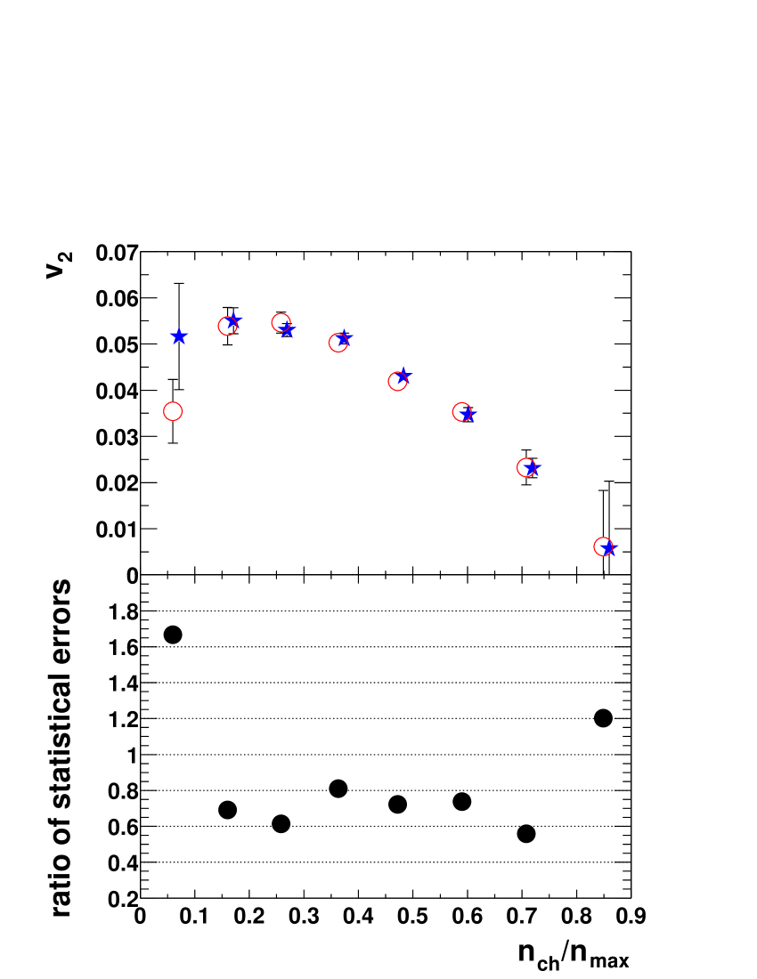
Figure 20: The upper panel shows measured $v_{2}$ from 4th-order cumulants versus centrality with $p_{t}$ weighting (stars) and unit weighting (circles). The bottom panel is the ratio of error from $p_{t}$ weighted $v_{2}$ to that of unit weighted $v_{2}$.

V Elliptic flow fluctuations

High precision results presented in this publication become sensitive to another effect usually neglected in flow analysis, namely, event-by-event flow fluctuations. The latter can have two different origins: “real” flow fluctuations — fluctuations at fixed impact parameter and fixed multiplicity (see, for example Kodama ) — and impact parameter variations among events from the same centrality bin in a case where flow does not fluctuate at fixed impact parameter. These effects, in principle, are present in any kind of analysis, including the “standard” one based on pair correlations. The reason is that any flow measurements are based on correlations between particles, and these very correlations are sensitive only to certain moments of the distribution in $v_{2}$. In the pair correlation approach with the reaction plane determined from the second harmonic, the correlations are proportional to $v^{2}$. After averaging over many events, one obtains $\langle v^{2}\rangle$, which in general is not equal to $\langle v\rangle^{2}$. The 4-particle cumulant method involves the difference between 4-particle correlations and (twice) the square of the 2-particle correlations. In this paper, we assume that this difference comes from correlations in the non-flow category. Note, however, that in principle this difference ($\langle v^{4}\rangle-\langle v^{2}\rangle^{2}\neq 0$) could be due to flow fluctuations. Let us consider an example where the distribution in $v$ is flat from $v=0$ to $v=v_{\rm max}$. Then, a simple calculation would lead to the ratio of the flow values from the standard 2-particle correlation method and 4-particle cumulants as large as $\langle v^{2}\rangle^{1/2}/(2\langle v^{2}\rangle^{2}-\langle v^{4}\rangle)^{1/4}=5^{1/4}\approx 1.5$.

In this study, we consider the possible bias in elliptic flow measurements under the influence of impact parameter fluctuations within the studied centrality bins. The largest effect is expected within the bin of highest multiplicity, where the impact parameter and $v_{2}$ are both known a priori to fluctuate down to zero in the limit of the most central collisions. These fluctuations lead to bin-width-dependent bias in the extracted $v_{2}$ measurements.

In section III, two approximations were made in order to extract the final flow result,

$$\langle v_{n}^{4}\rangle\simeq\langle v_{n}^{2}\rangle^{2}~{}~{}~{}~{}~{}~{}{\rm and}~{}~{}~{}~{}~{}~{}\langle v_{n}^{2}\rangle\simeq\langle v_{n}\rangle^{2}\,.$$

Taking into account the centrality binning fluctuation on flow, namely $\sigma_{v_{n}^{2}}^{2}$ and $\sigma_{v_{n}}^{2}$,

$$\langle v_{n}^{4}\rangle=\sigma_{v_{n}^{2}}^{2}+\langle v_{n}^{2}\rangle^{2}~{}~{}~{}~{}~{}~{}{\rm and}~{}~{}~{}~{}~{}~{}\langle v_{n}^{2}\rangle=\sigma_{v_{n}}^{2}+\langle v_{n}\rangle^{2}\,,$$

and Eq. (21) becomes

$$-v_{n}^{4}-2\sigma_{v_{n}}^{2}v_{n}^{2}-\sigma_{v_{n}}^{4}+\sigma_{v_{n}^{2}}^{2}=-v_{\rm meas}^{4}\,,$$ (29)

which is a function of $v_{n}$ and is solvable for $v_{n}$, if $\sigma_{v_{n}}^{2}$ and $\sigma_{v_{n}^{2}}^{2}$ are known. A method of calculating both $\sigma_{v_{n}}^{2}$ and $\sigma_{v_{n}^{2}}^{2}$ is now presented.

First, we need to parameterize $v_{n}$ as a function of impact parameter, $b$. Consider a polynomial fit $v_{n}=a_{0}+a_{1}b+...+a_{6}b^{6}$, in which case the measured flow is $\langle v_{n}\rangle=a_{0}+a_{1}\langle b\rangle+...+a_{6}\langle b^{6}\rangle$. The various averages $\langle b\rangle$, $\langle b^{2}\rangle$,… $\langle b^{12}\rangle$ can be estimated in each centrality bin from filtered HIJING events. The parameters $a_{i}$ have been determined by minimizing $\chi^{2}$ in a fit to the eight $v_{2}(n_{\rm ch})$ measurements. In addition, the fit is constrained to go through $v_{2}=0$ at $b=0$ and at $b_{max}=14.7$ fm Peter2000 . The variation of $b_{max}$ within $\pm 0.5$ fm has a negligible effect on $v_{2}(b)$ at $b<12$ fm. Fig. 21 shows the resulting curve:

$$v_{2}(b)=-0.000394\,b+0.00210\,b^{2}$$

$$-0.0000706\,b^{3}-0.0000320\,b^{4}+$$

$$0.00000358\,b^{5}-1.174\times 10^{-7}\,b^{6},$$ (30)

where it is assumed that $b$ is in fm. In principle, the final corrected $v_{2}(n_{\rm ch})$ should be determined iteratively, but the result is stable on the first iteration.

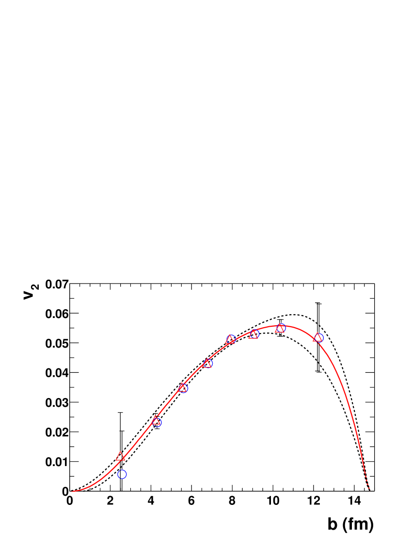
Figure 21: $v_{2}$ as a function of impact parameter. The data points are shown at the values of $\langle b\rangle$ for a given centrality bin. For the description of the fit procedure see text. The triangles are the final 4th-order cumulant data after correction for fluctuations as described in Section IV, while the circles show the 4th-order cumulant data before this correction. The dashed lines represent the estimated uncertainty in the parameterization represented by the solid curve.

Next we consider

$$\sigma_{v_{n}}^{2}=\langle v_{n}^{2}\rangle-\langle v_{n}\rangle^{2}=$$

$$(a_{0}^{2}+2a_{0}a_{1}\langle b\rangle+...\,a_{6}^{2}\langle b^{12}\rangle)-$$

$$(a_{0}+a_{1}\langle b\rangle+...\,a_{6}\langle b^{6}\rangle)^{2}\,,$$ (31)

and again the various averages of powers of $b$ can be estimated using HIJING.

After computing $\sigma_{v_{n}}^{2}$, $\sigma_{v_{n}^{2}}^{2}$, and obtaining $v_{\rm meas}$ from the four-particle correlation method, Eq. (29) can be solved to extract the $v_{n}$ corrected for impact parameter fluctuations. The $v_{2}$ bias is found to be entirely negligible in all the studied centrality bins except for the most central, where the correction is about a factor of two (see the leftmost bin in Fig. 21). In the present analysis, even a factor of two is not significant due to the large statistical error on $v_{2}$ for maximum centrality. However, the correction to $v_{2}$ resulting from finite centrality bin width at maximum centrality has been determined with lower uncertainty than $v_{2}$ itself, and will become important in future studies with large samples of events.

Real event-by-event fluctuation in the flow coefficients would also make the four-particle values lower than the two-particle values. At the moment, there is no way to calculate this effect, although it is expected to be small.

$\langle n_{ch}\rangle$	$\langle n_{ch}/n_{max}\rangle$	cross section	$\langle b\rangle$ (fm)	RMS ($b$)	$\langle{\varepsilon}\rangle$	$\langle v_{2}\rangle$
$53_{33}^{47}$	$0.060$	$53-77\%$	$12.23$	$0.99$	$0.420$	$0.052\pm 0.012$
$140_{40}^{40}$	$0.160$	$41-53\%$	$10.36$	$0.70$	$0.415$	$0.055\pm 0.003$
$227_{47}^{43}$	$0.258$	$31-41\%$	$9.06$	$0.68$	$0.371$	$0.053\pm 0.001$
$319_{49}^{41}$	$0.363$	$24-31\%$	$7.91$	$0.64$	$0.319$	$0.051\pm 0.001$
$415_{55}^{45}$	$0.472$	$16-24\%$	$6.80$	$0.70$	$0.261$	$0.043\pm 0.001$
$519_{59}^{41}$	$0.590$	$10-16\%$	$5.56$	$0.72$	$0.197$	$0.035\pm 0.002$
$622_{62}^{38}$	$0.708$	$5-10\%$	$4.26$	$0.80$	$0.131$	$0.023\pm 0.002$
$746_{86}^{124}$	$0.849$	top $5\%$	$2.53$	$1.00$	$0.058$	$0.012\pm 0.015$

Table 1: Tabulated values of observed charged particle multiplicity, $n_{ch}/n_{max}$, centrality in terms of percent of total geometric cross section, impact parameter with spread (root mean square) inferred from HIJING, the initial spatial anisotropy ${\varepsilon}$, and the final corrected elliptic flow based on 4th-order cumulants.

VI The centrality dependence of elliptic flow

The centrality dependence of elliptic flow is a good indicator of the degree of equilibration reached in the reaction VoloshinCentPhyV2 ; NA49QM . Following Ref. Peter2000 , we compute the initial spatial eccentricity for a Woods-Saxon distribution with a wounded nucleon model from

$${\varepsilon}=\frac{\langle y^{2}\rangle-\langle x^{2}\rangle}{\langle y^{2}\rangle+\langle x^{2}\rangle}\,$$

where $x$ and $y$ are coordinates in the plane perpendicular to the beam and $x$ denotes the in-plane direction. The method of calculation of epsilon is the same as used for the hydro valuesKolb00 . The ratio $v_{2}/{\varepsilon}$ is of interest because it has been argued to be independent of centrality in a hydrodynamic model with constant speed of sound Olli92 . In hydrodynamic model calculations using an equation of state with a phase transition (sound speed is not constant) this ratio does change as a function of centrality, however within the $10\%$ level Kolb00 . Hydrodynamics represents one possible limiting case in describing nuclear collisions — the limit where the mean free path for interaction of the constituents represented by the fluid cells is very small compared with the region of nuclear overlap. The opposite limit, where the mean free path is long (or at least comparable to the dimensions of the nuclear overlap region) is normally known as the Low Density Limit (LDL). In nuclear transport models, the mean number of hard binary interactions per particle is typically small, and the predictions of these models tend to be closer to the low density limit than the hydro limit. In order to judge the proximity of measured flow data to either of these limits, it is useful to plot, as in Fig. 22, $v_{2}/{\varepsilon}$ versus charged particle density in the form $(dN/dy)/S$, where $dN/dy$ is rapidity density, and the area of the overlap region is $S=\pi\sqrt{\langle x^{2}\rangle\langle y^{2}\rangle}$ as computed above. Since $v_{2}/{\varepsilon}$ is proportional to $(dN/dy)/S$ in the LDL case Heiselberg ; VoloshinCentPhyV2 , this form of plot offers meaningful insights without reference to detailed theoretical models.

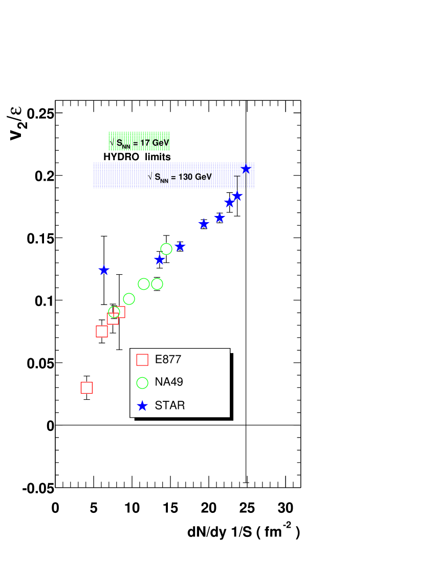
Figure 22: $v_{2}/{\varepsilon}$ as a function of charged particle density in Au + Au collisions. Data are from E877 at the AGS (squares), NA49 at the SPS (circles), and STAR at RHIC (stars). The AGS and SPS data have been obtained by conventional flow analysis. The STAR measurements are at $\sqrt{s_{NN}}=130$ GeV, and correspond to the final corrected elliptic flow based on 4th-order cumulants, and we assume $dN/dy=1.15dN/d\eta$. The horizontal shaded bands indicate the hydrodynamic limits for different beam energiesKolb00 .

Figure 22 presents Au + Au data from AGS/E877 Barr95 , from NA49 NA49QM , as well as the current STAR measurements based on 4th-order cumulants, corrected for fluctuations as detailed in Section IV. Alternative forms of the centrality dependence readily can be generated using the tabulated quantities presented in Table I. Generally, the current STAR results underline the need for much increased statistics, particularly for the most central collisions. Within the uncertainties, a smooth trend of increasing $v_{2}/{\varepsilon}$ with increasing centrality (larger $(dN/dy)/S$) is observed, without the obvious kink that has been suggested as a phase transition signature Sorge99 ; Heiselberg . Another proposed phase transition signature which is not favored by the data is a few percent rise in $v_{2}/{\varepsilon}$ with decreasing centrality Kolb00 . It is noteworthy that the $v_{2}/{\varepsilon}$ values reached in the most central RHIC collisions are consistent with the hydrodynamic limit Olli92 ; Kolb99 ; Kolb00 , whereas $v_{2}/{\varepsilon}$ in central collisions at AGS and SPS is significantly lower. It is also worthy of note that while the roughly linear relationship between $v_{2}/{\varepsilon}$ and $(dN/dy)/S$ across the presented beam energies and centralities is consistent with the LDL picture Heiselberg , the measured $v_{2}(p_{t})$ Fig. 15 cannot be explained by current LDL implementations Kolb01 , and is much closer to hydrodynamic calculations up to 2 GeV$/c$ Kolb01 .

VII Conclusion

In this work, we provide details of the approach for treating non-flow correlations within the framework of the standard elliptic flow analysis method based on particle pairs. We also compare the standard method with a new and simpler pair analysis based on the scalar product of flow vectors. The latter yields a 15 – 35% reduction in statistical errors, with the best improvement occurring in the case of the most central and the most peripheral events.

It is concluded that four-particle correlation analyses can reliably separate flow and non-flow correlation signals, and the latter account for about 15% of the observed second-harmonic azimuthal correlation in year-one STAR data. The cumulant approach has demonstrated some advantages over the previous alternatives for treating non-flow effects. In particular, 4th-order cumulants allows us to present $v_{2}$ measurements fully corrected for non-flow effects, in contrast to the earlier analyses where the non-flow contribution was partly removed and partly quantified by the reported systematic uncertainties. It is observed that non-flow correlations are present in $\sqrt{s_{NN}}=130$ GeV Au + Au events throughout the studied region $|\eta|<1.3$ and $0.1<p_{t}<4.0$ GeV/$c$, and are present at all centralities. The largest contribution from non-flow correlations is found among the most peripheral and the most central collisions.

On the other hand, a 4th-order cumulant analysis is subject to larger statistical errors than a conventional pair correlation analysis of the same data set. The total uncertainty on the 4th-order analysis, including both statistical and systematic effects, is smaller for year-one STAR data except in the most central and peripheral panels of Figs. 14 and 15. In the case of future studies of larger numbers of events, a higher-order analysis should provide an advantage in all cases.

Fluctuations within the studied multiplicity bins have the potential to bias elliptic flow results. This bias has been estimated and found to be entirely negligible except for the most central multiplicity bin, where the correction is about a factor of two. In the present analysis, even this large a bias is only marginally significant, but again, this correction will presumably be important in future studies with much improved statistics.

We present STAR data for $v_{2}/{\varepsilon}$ — elliptic flow in various centrality bins, divided by the initial spatial eccentricity for those centralities. Mapping centrality onto a scale of charged particle density enables us to study a broad range of this quantity, from peripheral AGS collisions, through SPS, and ending with central RHIC collisions. Within errors, the STAR data follow a smooth trend. No evidence for a softening of the equation of state or for a change in degrees of freedom has been observed. The three experiments at widely differing beam energies show good agreement in $v_{2}/{\varepsilon}$ where they overlap in their coverage of particle density. The pattern of $v_{2}/{\varepsilon}$ being roughly proportional to particle density continues over the density range explored at RHIC, which is consistent with a general category of models which approximate the low density limit as opposed to the hydrodynamic limit. Nevertheless, $v_{2}/{\varepsilon}$ at STAR is consistent with having just reached the hydrodynamic limit for the most central collisions.

- (1) W. Reisdorf, and H. G. Ritter, Annu. Rev. Nucl. Part. Sci. 47, 663 (1997).
- (2) N. Herrmann, J. P. Wessels, and T. Wienold, Annu. Rev. Nucl. Part. Sci. 49, 581 (1999).
- (3) J.-Y. Ollitrault, Nucl. Phys. A638, 195c (1998).
- (4) A. M. Poskanzer, e-print nucl-ex/0110013 (2001).
- (5) H. Sorge, Phys. Rev. Lett. 78, 2309 (1997).
- (6) J.-Y. Ollitrault, Phys. Rev. D46, 229 (1992).
- (7) S. Voloshin and Y. Zhang, Z. Phys. C70, 665 (1996).
- (8) A. M. Poskanzer and S. A. Voloshin, Phys. Rev. C58, 1671 (1998).
- (9) STAR collaboration, K. H. Ackermann et al., Phys. Rev. Lett. 86, 402 (2001).
- (10) D. Teaney, J. Lauret, and Edward V. Shuryak, Nucl. Phys. A698, 479 (2002).
- (11) D. Teaney, J. Lauret, and Edward.V. Shuryak, e-print nucl-th/0110037
- (12) Zi-wei Lin and C. M. Ko, Phys. Rev. C65, 034904 (2002).
- (13) C. M. Ko, Zi-wei Lin, and S. Pal, e-print nucl-th/0205056 (2002).
- (14) D. Molnar and M. Gyulassy, Nucl. Phys. A697, 495 (2002).
- (15) E.E. Zabrodin, C. Fuchs, L.V. Bravina, and A. Faessler, Phys. Lett. B508, 184 (2001).
- (16) T. J. Humanic, e-print nucl-th/0205053.
- (17) STAR collaboration, C. Adler et al., Phys. Rev. Lett. 87, 182301 (2001).
- (18) H. Heiselberg and A.-M. Levy, Phys. Rev. C59, 2716 (1999).
- (19) J. Jiang et al., Phys. Rev. Lett. 68, 2739 (1992).
- (20) N. Borghini, P. M. Dinh, and J.-Y. Ollitrault, Phys. Rev. C63, 054906 (2001).
- (21) N. Borghini, P. M. Dinh, and J.-Y. Ollitrault, Phys. Rev. C64, 054901 (2001).
- (22) STAR collaboration, K. H. Ackermann et al., Nucl. Phys. A661, 681c (1999).
- (23) P. Danielewicz and G. Odyniec, Phys. Lett. B157, 146 (1985).
- (24) M. Gyulassy and X.-N. Wang, Comput. Phys. Commun. 83, 307 (1994); X.N. Wang and M. Gyulassy, Phys. Rev. D44, 3501 (1991).
- (25) P. Danielewicz, Phys. Rev. C51, 716 (1995).
- (26) A. M. Poskanzer and S. A. Voloshin, LBNL Annual Report http://ie.lbl.gov/nsd1999/rnc/RNC.htm R34 (1998).
- (27) E877 collaboration, J. Barrette et al., Phys. Rev. Lett. 73, 2532 (1994);
- (28) J.-Y. Ollitrault, Nucl. Phys. A590, 561c (1995).
- (29) J.-Y. Ollitrault, e-print nucl-ex/9711003 (1997).
- (30) N. Borghini, P. M. Dinh, and J.-Y. Ollitrault, Phys. Rev. C62, 034902 (2000).
- (31) P. M. Dinh, N. Borghini, and J.-Y. Ollitrault, Phys. Lett. B477, 51 (2000).
- (32) M. Biyajima, Phys. Lett. B92, 193 (1980); Prog. Theor. Phys. 66, 1378 (1981).
- (33) R. L. Liboff, Kinetic Theory Prentice Hall, Englewood Cliffs, New Jersey (1989).
- (34) H. C. Eggers, P. Lipa, P. Carruthers, and B. Buschbeck, Phys. Rev. D48, 2040 (1993).
- (35) N. Borghini, P. M. Dinh, and J.-Y. Ollitrault, e-print nucl-ex/0110016.
- (36) R. L. Ray and R. S. Longacre, STAR Note SN0419, 1999, e-print nucl-ex/0008009.
- (37) STAR collaboration, R. Snellings et al., Quark Matter, (2001).
- (38) M. Gyulassy, I. Vitev, and X. N. Wang, Phy. Rev. Lett. 86, 2537 (2001).
- (39) STAR collaboration, C. Adler et al., in preparation.
- (40) C.E. Aguiar et al., Nucl. Phys. A698, 639c (2002).
- (41) P. Jacobs and G. Cooper, STAR Note SN0402, 1999, e-print nucl-ex/0008015.
- (42) S. A. Voloshin and A. M. Poskanzer, Phys. Lett. B474, 27 (2000).
- (43) A. M. Poskanzer and S. A. Voloshin, Nucl. Phys. A661, 341c (1999).
- (44) P. F. Kolb, J. Sollfrank, and U. Heinz, Phys. Rev. C62, 054909 (2000).
- (45) E877 collaboration, J. Barrette et al., Phys. Rev. C51, 3309 (1995); C55, 1420 (1997).
- (46) H. Sorge, Phys. Rev. Lett. 82, 2048 (1999).
- (47) P. Kolb, J. Sollfrank, and U. Heinz, Phys. Lett. B459, 667 (1999).
- (48) P.F. Kolb, P. Huovinen, U. Heinz, and H. Heiselberg, Phys. Lett. B500, 232 (2001).