Measurement of the $\eta$ Production in Proton Proton Collisions with the COSY Time of Flight Spectrometer

Abstract

The reaction pp $\rightarrow$ pp$\eta$ was measured at excess energies of 15 and 41 MeV at an external target of the Jülich Cooler Synchrotron COSY with the Time of Flight Spectrometer. About 25000 events were measured for the excess energy of 15 MeV and about 8000 for 41 MeV. Both protons of the process pp$\eta$ were detected with an acceptance of nearly 100 % and the $\eta$ was reconstructed by the missing mass technique. For both excess energies the angular distributions are found to be nearly isotropic. In the invariant mass distributions strong deviations from the pure phase space distributions are seen.

1 Introduction

The production of $\eta$ mesons in nucleon-nucleon collisions has attracted a considerable attention in the last years [1]..[6]. Due to the relatively high mass of the $\eta$ meson its production requires a large momentum transfer between the initial and final states. At threshold this momentum transfer is given by $q=\sqrt{(}m_{N}m_{\eta}+\frac{1}{4}m_{\eta}^{2})$, where $m_{N}$ and $m_{\eta}$ are the nucleon and $\eta$ meson masses, and amounts to 770 MeV/c. This large momentum transfer translates into a short distance between the two interacting nucleons ($\sim 0.26$ fm). Therefore $\eta$ production permits the investigation of short range hadron dynamics and provides a tool to probe the behavior of nucleon-nucleon interaction at small distances. The mechanism of $\eta$ production in nucleon-nucleon collisions is yet not well understood. As the $\eta$ meson couples strongly to the $S_{11}$(1535 MeV), it has been assumed that this resonance is predominantly involved in its production. The mechanism of the excitation of this resonance in hadronic collisions remains in turn an open question. As the dominant excitation mechanism both $\pi$ and $\eta$ exchange have been assumed [7]. According to other calculations however, $\rho$ meson exchange is supposed to be responsible mainly for the excitation of the $S_{11}$ resonance [8], [9]. The shape of the angular distribution in the $pp\rightarrow pp\eta$ reaction reflects the properties of the exchanged meson in the excitation of the $S_{11}$ resonance. In Ref. [10] it is shown that in spite of the dominance of the resonance amplitude the effects of relatively small mesonic currents can be seen in the shape of the $\eta$ angular distribution due to interference. On the other hand, according to a recent approach [11] the $S_{11}$ resonance is less involved in the production of the $\eta$ meson. In this approach the $\eta$ meson production is mainly due to the short range amplitude of the nucleon-nucleon interaction. As the $\eta$ is the lightest meson containing $s\overline{s}$ quarks the question of direct production channels is interesting because it may be related to the $s\overline{s}$ content of the proton. The production of the $\eta$ meson also poses another interesting aspect. The $\eta$ meson interacts strongly with the nucleon and in its production the final state $\eta$-nucleon interaction should play an important role. The near threshold dependence of the observed total cross section for $\eta$ production differs substantially from that for $\pi$ and $\eta^{\prime}$ production, pointing to an enhancement of the measured cross section which can be ascribed to a strong attraction in $\eta$-nucleon interaction [12].

More data of improved precision will undoubtedly contribute to a better understanding of the $pp\rightarrow pp\eta$ reaction.

2 Experiment

The external proton beam with a diameter of 1-2 mm impinges on a 4 mm thick liquid hydrogen target enclosed with plastic foils of only 0.9 $\mu m$ thickness [13]. The start and stop counters have azimuthal symmetry with holes for the beam such that only reaction particles hit the counters. Three scintillators with holes of 8 mm, 5 mm and 2 mm diameter placed 1 m, 0.5 m and 10 cm in front of the target are used to veto the beam halo. The incident beam and the whole detection system are enclosed in vacuum in order to minimize multiple scattering and secondary reactions (Fig. 1).

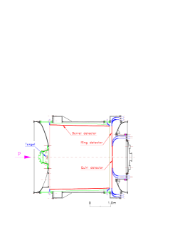
Figure 1: The experimental set up of the COSY-TOF detector. A cross section through the cylindrical detector is shown.

A 0.5 mm thick scintillator counter is used as start counter. It has an inner hole of 3 mm diameter and is arranged in two cones each of 16 individual counters [14]. The stop counters are divided into the inner part (quirl counter with 96 channels in 3 layers[15]), the ring counter with 192 channels in 3 layers and the barrel counter with 192 channels [16]. The high granularity of the stop scintillators results in a resolution for the azimuthal angle of $2^{\circ}$ - $4^{\circ}$ and for the polar angle of typically $0.5^{\circ}$. The acceptance for charged particles in $\phi$ is $2\pi$, for $\theta$ it ranges from $0.8^{\circ}$ - $75^{\circ}$. The time of flight is measured with a resolution of 1% of the typical time of flight for protons of the $pp\rightarrow pp\eta$ reaction close to threshold. For the measurement with a beam momentum of 2025 MeV/c (corresponding to an excess energy $\epsilon$ of the pp$\eta$ system of 15 MeV) the trigger condition was to measure at least two charged tracks in the quirl and at least one charged track in the start counter. For the beam momentum of 2100 MeV/c ($\epsilon$ = 41 MeV) the charged tracks in the ring counter were added to the trigger in order to take into account the larger opening angle of the protons.

3 Data Analysis

The $\eta$ is reconstructed from the tracks of both protons. For each track the particle momentum is calculated from the time of flight and the measured directions with the mass of the proton assumed. The missing mass is calculated from momentum and energy conservation as

$$m_{x}^{2}=(\mathbb{P}_{beam}+\mathbb{P}_{target}-\mathbb{P}_{track1}-\mathbb{P}_{track2})^{2}$$

$\mathbb{P}$ is the four momentum of the particles. Only two charged track events are taken into account, such that events with the $\eta$ decaying into charged particles hitting the ring or quirl counter are discarded. Pion tracks result in very low or negative squared missing masses if the mass of the proton is assumed. Near the kinematical limit, which corresponds to a missing mass of 562.5 MeV/$c^{2}$ ($\epsilon$ =15 MeV) and 588.5 MeV/$c^{2}$ ($\epsilon$ =41 MeV), only proton tracks from pp$\eta$ and multi-pion production events are contributing. In order to reduce the amount of background events, a first selection on the squared missing mass is applied ($m_{x}^{2}>0.2$ $GeV^{2}/c^{4}$). This cut and the condition on the particle time of flight corresponding to velocities of $0<\beta<1$ are the only cuts applied in the analysis.

The measured data are compared with simulated data obtained with a Monte Carlo program, which is based on the GEANT3 code. It generates a data sample which is analyzed using the same evaluation routines as for the measured data. As time resolution for each layer of the scintillation counters 250 ps ($\sigma$) for the stop counters and 150 ps ($\sigma$) for the start counters was determined. The width of the $\eta$ signal in the missing mass distribution is well reproduced for both excess energies (Fig. 2).

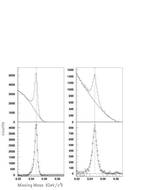
Figure 2: The missing mass distribution for the excess energy of 15 MeV (first column) and 41 MeV (second column). Upper figure: Raw data with fitted background. Lower figure: Missing mass distribution from Monte Carlo calculations (solid line) in comparison with data after background subtraction (crosses).

The width of the $\eta$ signal is 0.8% (FWHM) of the $\eta$ mass for $\epsilon$=15 MeV and 1.3% for $\epsilon$=41 MeV. The overall reconstruction efficiency including the acceptance and the constraint of having no charged pions of the $\eta$ decay in the forward detector was 68% for $\epsilon$=15 MeV and 69% for $\epsilon$=41 MeV. The distribution of the invariant proton-proton mass is parameterized by the measured distribution and used instead of the pure phase space as input for the Monte Carlo calculation. This influences the Monte Carlo results mainly at forward - backward $\eta$-directions for the lower excess energy.

The normalization of the angular distributions affected by this correction amounts to less than 10 % (s. Fig. 3). For the excess energy of 41 MeV this correction is less than 2%.

Figure 3: Monte Carlo results: Acceptance and reconstruction efficiency as a function of $cos(\theta_{\eta}^{cm})$.

The pp$\eta$ system in the final state is described by 12 variables, of which 7 are fixed by momentum and energy conservation and the particle masses. 2 variables are given by the invariant masses $M_{pp}$ and $M_{p\eta}$. The remaining 3 variables describe the orientation of the pp$\eta$ system with respect to the incoming proton axis. For these variables we choose the angle of the $\eta$ momentum in the center of mass frame with respect to the beam axis ($\theta_{\eta}^{cm}$) and the angle of the relative momentum of the proton proton system to the beam axis ($\theta_{q}^{cm}$). The remaining variable is the azimuthal orientation, which is of no significance in this unpolarized measurement.

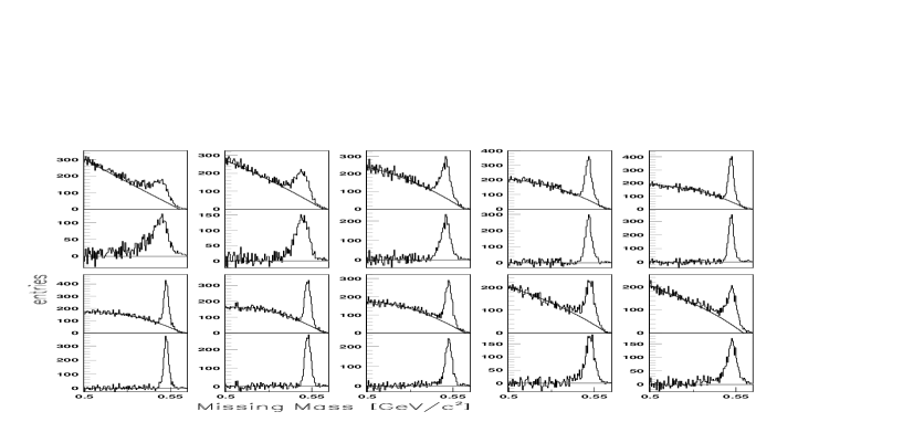
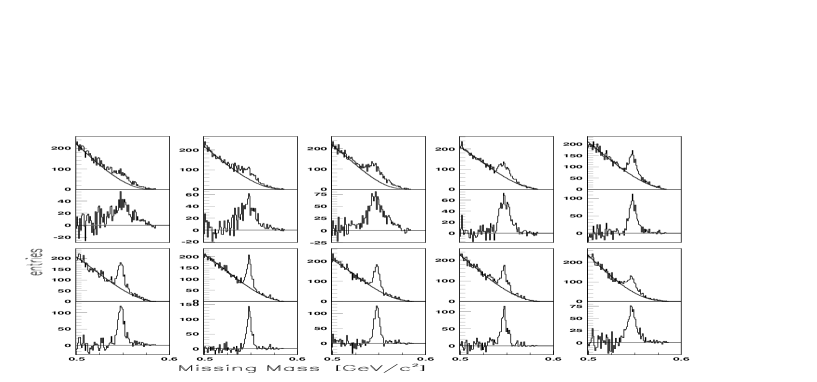
Figure 12: The missing mass distribution for bins of $cos(\theta_{\eta}^{cm})$ ($\epsilon$=15 MeV, upper part and $\epsilon$ =41 MeV, lower part). The first row shows the data with the fit of the background for $cos(\theta_{\eta}^{cm})$ in the range from -1. to 0. in steps of .2, the second row shows the $\eta$ signal which is obtained by subtracting the fitted background. The third and fourth rows show the corresponding bins of $cos(\theta_{\eta}^{cm})$ in the range from 0. to 1.

In order to obtain differential cross sections with respect to the quantities $M^{2}_{pp}$, $M^{2}_{p\eta}$, $cos(\theta_{\eta}^{cm})$, and $cos(\theta_{q}^{cm})$ for $pp\rightarrow pp\eta$ the continuum background in the pp missing mass has to be subtracted. The procedure is illustrated in the appendix, in case of $cos(\theta_{\eta}^{cm})$ in Fig. 12. For each of 10 equidistant bins between $cos(\theta_{\eta}^{cm})=-1$ and $cos(\theta_{\eta}^{cm})=+1$ pp missing mass spectra were generated. In each missing mass distribution the number of $\eta$ events is determined by fitting a polynomial of 3rd degree to the background and a Gaussian distribution to the $\eta$ signal. The fit is done recursively by removing the fitted signal from the overall measured distribution and fitting the background again. The width of the $\eta$ signal in the missing mass varies with the center of mass angle of the $\eta$ due to the corresponding different velocities of the protons resulting in different missing mass resolutions. Therefore the limits for integrating the $\eta$ signal are varying. These limits are determined from the width of the $\eta$ signal of Monte Carlo calculations.

In the same way differential cross section distributions for $M^{2}_{pp}$, $M^{2}_{p\eta}$, and $cos(\theta_{q}^{cm})$ were obtained by fitting background and $\eta$ peak in the pp missing mass and subtracting the background as a function of $M^{2}_{pp}$ ,$M^{2}_{p\eta}$, and $cos(\theta_{q}^{cm})$ respectively.

The angular distributions are normalized to the total cross sections of 2.11 $\mu b$ ($\epsilon$=15 MeV) and 4.92 $\mu b$ ($\epsilon$=41 MeV) which are taken from Ref. [3].

In Figs. 4-11 only statistical errors are plotted. The systematic errors are given in the appendix in tables 2-4. The estimated systematic error is composed of a constant term due to possible angular dependent detector and reconstruction inefficiencies ($\pm$5%) and of a term which is proportional to the width of the $\eta$ signal in the missing mass, in order to reflect the error due to the separation of the signal from background ($\pm$2%$\cdot$FWHM[MeV/$c^{2}$]).

4 Angular Distributions

The angular distribution of the $\eta$ in the center of mass system is evaluated as described above. This procedure allows in addition for the examination of the background behavior, which is shown in Fig. 4.

Figure 4: Number of background events as a function of the cosine of the $\eta$ angle.

The angular distribution of the background, which is measured for a constant range in the missing mass spectrum, deviates from isotropy.

The efficiency and acceptance corrected $\eta$ angular distributions for $\epsilon$=15 MeV and 41 MeV are shown in Fig. 5.

Figure 5: Angular distribution of the $\eta$ in the center of mass frame.

Within the statistical errors both distributions show no deviation from isotropy. The forward-backward symmetry in the center of mass frame required by the initial state consisting of two identical particles has not been used as a constraint in the data evaluation.

The second variable describing the orientation of the pp$\eta$ system is the angle $\theta_{q}^{cm}$. The relative momentum between both protons in the overall center of mass frame is given by:

$$\vec{q}=\frac{1}{2}\cdot(\vec{p}\,^{cm}_{proton_{1}}-\vec{p}\,^{cm}_{proton_{2}})$$

The sequence of first and second proton is randomized for evaluating the angular distribution which is shown in Fig. 6.

Figure 6: Angular distribution of the relative p p momentum in the center of mass frame.

As in the case of the $\eta$ angular distribution these differential cross sections are consistent with isotropy.

5 Invariant Mass Distributions

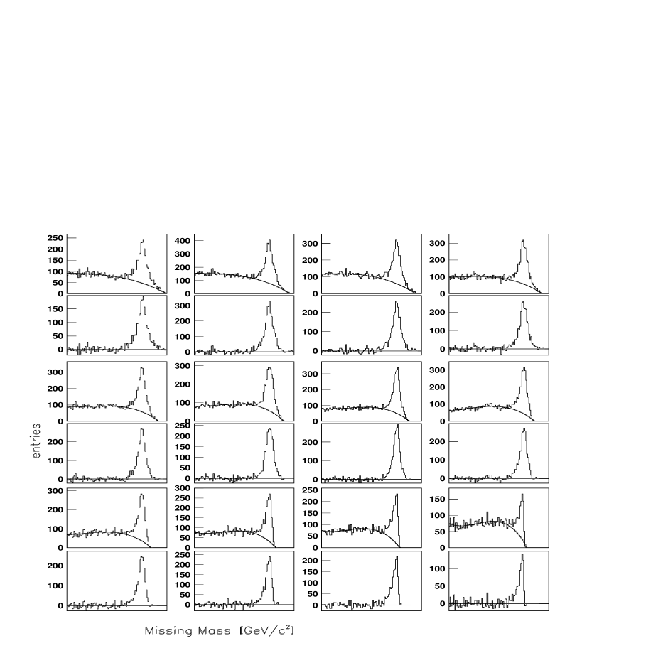
Figure 13: The missing mass distribution for bins of the proton-proton invariant mass at $\epsilon=15$ MeV. The upper histogram shows the data including the fit of the background. Beneath this histogram the $\eta$ signal is shown, which is obtained by subtracting the fitted background. Each histogram represents a bin in $M^{2}_{pp}$ in the range from 3.52 to 3.57 $GeV^{2}/c^{4}$ in steps of .005 $GeV^{2}/c^{4}$.

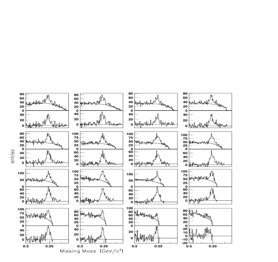
Figure 14: The missing mass distribution for bins of the proton-proton invariant mass at $\epsilon=41$ MeV. The upper histogram shows the data including the fit of the background. Beneath this histogram the $\eta$ signal is shown, which is obtained by subtracting the fitted background. Each histogram represents a bin in $M^{2}_{pp}$ in the range from 3.52 to 3.68 $GeV^{2}/c^{4}$ in steps of .01 $GeV^{2}/c^{4}$.

The invariant mass distributions are evaluated as explained in chapter 4. The sequence of missing mass spectra is shown in Figs. 13,14 in the appendix. The squared proton-proton invariant mass is given by

$$M_{pp}^{2}=(\mathbb{P}_{track_{1}}+\mathbb{P}_{track_{2}})^{2}$$

The efficiency and acceptance corrected proton-proton invariant mass distributions are shown in Fig.7.

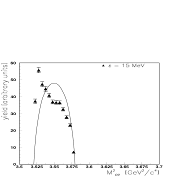
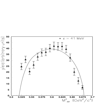
Figure 7: Squared proton-proton invariant mass distribution (upper Figure: excess energy of 15 MeV, lower Figure: excess energy of 41 MeV). The solid points show the efficiency and acceptance corrected data. The line represents the pure phase space.

The invariant mass of the proton - $\eta$ system is given by

$$M_{p\eta}^{2}=(\mathbb{P}_{\eta}+\mathbb{P}_{track_{1,2}})^{2}$$

The four momentum of the $\eta$ particle is calculated from the momentum

$$\vec{p}_{\eta}=\vec{p}_{beam}-\vec{p}_{track_{1}}-\vec{p}_{track_{2}}$$

and from the total energy

$$E=\sqrt{(p_{\eta}^{2}+m_{\eta}^{2})}$$

For $m_{\eta}$ the exact mass (.5475 GeV/$c^{2}$) is taken. As the protons of the final state are not distinguishable the invariant mass $M_{p\eta}^{2}$ is evaluated twice for each event by exchanging track 1 with track 2.

The proton-$\eta$ invariant mass distributions, which are deduced in the same way as the proton-proton invariant mass distributions, are shown in Fig. 8.

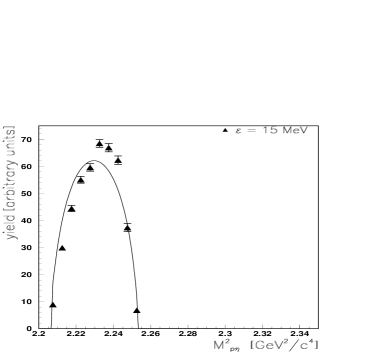
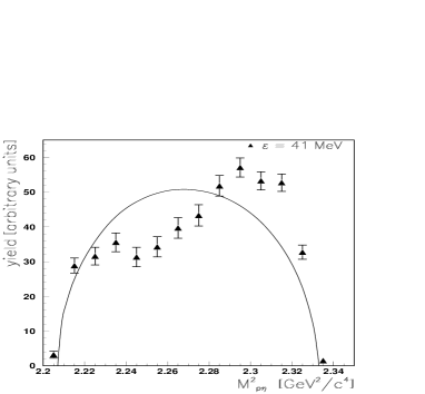
Figure 8: Squared proton-$\eta$ invariant mass distribution (upper Figure: excess energy of 15 MeV, lower Figure: excess energy of 41 MeV). The solid points show the efficiency and acceptance corrected data. The line represents the pure phase space.

The numerical values are listed in the appendix in tables 3, 4. The systematic errors are calculated as explained in section 3.

6 Discussion

The angular distributions at the excess energy of $\epsilon$=41 MeV were fitted with a function containing a $cos^{2}\theta$ dependence: $c_{1}+c_{2}\cdot cos^{2}\theta$. For the $cos\theta_{\eta}$ distribution the results were $c_{1}=0.396\pm 0.009$ and $c_{2}=-0.011\pm 0.032$, for the $cos\theta_{q}$ distribution the results were $c_{1}=0.386\pm 0.014$ and $c_{2}=0.018\pm 0.035$. This means that the measured angular distributions are isotropic and therefore consistent with s-wave behavior.

This is in contradiction to the results from CELSIUS [5] which are based on a data sample of lower statistical significance: a factor of 80 (10) smaller for the lower (higher) excess energy. The data are compared with our results in Figs. 9, 10. At the higher excess energy close to $\epsilon$=40 MeV the shapes of the angular distributions are in disagreement, particularly at the most forward and backward angles.

Theoretical predictions for the angular distribution of G. Fäldt, C. Wilkin [9] and K. Nakayama [10] are shown in Fig. 10. In both calculations the excitation of the $S_{11}$ resonance is the dominant term. In the model of Ref. [10] the $\pi$- and $\eta$ exchange is the largest contribution of the resonance excitation, while in Ref. [9] $\rho$ exchange is dominating. While the results of both calculations show nearly the same shape (solid line in Fig. 10), the origin of this shape is different. In Ref. [10] it arises from an interference between the very small non resonant meson exchange process with the resonance excitation process, which - if taken alone - produces an inverted shape as shown by the dashed line in Fig. 10. In Ref. [9] it is argued that this shape is due to the $\rho$ exchange of the resonance excitation and that a dominant $\pi$ exchange will invert the shape.

Within the statistical and systematical error neither of the calculations can be excluded by the data.

The invariant mass distributions exhibit large deviations from the pure phase space as shown in Figs. 7,8, and in Fig. 11, where the data are normalized to the phase space. The first maximum in the proton-proton invariant mass spectrum is due to the pp final state interaction. The effect, that a second maximum is seen for $\epsilon$ = 41 MeV is a surprising result and cannot be explained by an interplay of pp FSI and phase space distribution alone. In the proton-$\eta$ distribution a clear shift to higher energies compared to phase space is observed. An enhancement towards higher invariant masses is expected either by a Breit - Wigner parameterization for the $S_{11}(1535)$ or by a FSI approach with a positive scattering length for the proton - $\eta$. But as simple weight factors they cannot describe the strong modulations in the invariant proton - $\eta$ mass spectrum. The Dalitz plot occupation probably has to be parameterized by amplitude contributions in the 3 two body subsystems taking care of interference effects.

Figure 9: Comparison of the measured angular distribution with the measurement of CELSIUS [5] close to $\epsilon$=15 MeV

Figure 10: Comparison of the measured angular distribution with the measurement of CELSIUS [5] close to $\epsilon$=40 MeV. The solid line represents calculations from Refs. [9], [10], the dashed line shows the calculation from Ref. [10] by only taking the resonance excitation into account.

Figure 11: Ratio of the acceptance corrected measured invariant mass distribution and the pure phase space. Upper figure: proton-proton invariant mass, lower figure: proton-$\eta$ invariant mass

7 Conclusion

The high statistics and high acceptance measurements of the $pp\rightarrow pp\eta$ reaction were performed with the COSY-TOF spectrometer. Kinematically complete events were obtained. They allow for detailed analysis of all possible observables. The differential cross sections of $\eta$ with respect to the beam direction show that up to 40 MeV excess energy the $\eta$ is still produced purely in s-wave. There are deviations of the invariant mass distributions from the pure phase, which cannot be explained by pp FSI alone.

8 Acknowledgment

We thank the COSY Crew for delivering a stable and high quality proton beam. This work has been supported by the FFE fond of the Forschungszentrum-Jülich, by the European Community - Access to Research Infrastructure action of the Improving Human Potential Programme, and by the German BMBF. One of us (P.Z.) wishes to thank Polish State Committee for Scientific Research for a partial support under grant KBN 3P 03B 04521.

9 Appendix

Table 1: Angular distribution of the $\eta$ momentum in the cm system

	$\epsilon$ = 15 MeV			$\epsilon$ = 41 MeV
$cos(\theta_{\eta}^{cm})$
	$\frac{d\sigma}{d\Omega}$[$\mu$b/sr]	stat. error	sys. error	$\frac{d\sigma}{d\Omega}$[$\mu$b/sr]	stat. error	sys. error
-0.9	0.168	$\pm$ 0.007	$\pm$0.018	0.366	$\pm$0.033	$\pm$0.068
-0.7	0.163	$\pm$ 0.006	$\pm$0.015	0.383	$\pm$0.033	$\pm$0.064
-0.5	0.172	$\pm$ 0.006	$\pm$0.013	0.402	$\pm$0.032	$\pm$0.055
-0.3	0.173	$\pm$ 0.005	$\pm$0.011	0.357	$\pm$0.030	$\pm$0.040
-0.1	0.173	$\pm$ 0.005	$\pm$0.011	0.376	$\pm$0.026	$\pm$0.035
+0.1	0.168	$\pm$ 0.005	$\pm$0.010	0.432	$\pm$0.024	$\pm$0.036
+0.3	0.159	$\pm$ 0.005	$\pm$0.009	0.379	$\pm$0.027	$\pm$0.030
+0.5	0.165	$\pm$ 0.006	$\pm$0.010	0.398	$\pm$0.027	$\pm$0.034
+0.7	0.170	$\pm$ 0.006	$\pm$0.012	0.436	$\pm$0.032	$\pm$0.042
+0.9	0.167	$\pm$ 0.006	$\pm$0.013	0.387	$\pm$0.029	$\pm$0.045

Table 2: Angular distribution of the relative momentum of the protons in the cm system

	$\epsilon$ = 15 MeV			$\epsilon$ = 41 MeV
$cos(\theta_{q}^{cm})$
	$\frac{d\sigma}{d\Omega}$[$\mu$b/sr]	stat. error	sys. error	$\frac{d\sigma}{d\Omega}$[$\mu$b/sr]	stat. error	sys. error
-0.9	0.162	$\pm$0.007	$\pm$0.014	0.420	$\pm$0.036	$\pm$0.065
-0.7	0.153	$\pm$0.006	$\pm$0.012	0.413	$\pm$0.029	$\pm$0.056
-0.5	0.158	$\pm$0.006	$\pm$0.012	0.363	$\pm$0.028	$\pm$0.044
-0.3	0.182	$\pm$0.006	$\pm$0.014	0.375	$\pm$0.028	$\pm$0.041
-0.1	0.181	$\pm$0.006	$\pm$0.013	0.378	$\pm$0.028	$\pm$0.041
+0.1	0.183	$\pm$0.006	$\pm$0.014	0.380	$\pm$0.027	$\pm$0.041
+0.3	0.175	$\pm$0.006	$\pm$0.013	0.417	$\pm$0.028	$\pm$0.047
+0.5	0.161	$\pm$0.006	$\pm$0.013	0.403	$\pm$0.029	$\pm$0.049
+0.7	0.161	$\pm$0.006	$\pm$0.013	0.415	$\pm$0.030	$\pm$0.056
+0.9	0.165	$\pm$0.007	$\pm$0.014	0.352	$\pm$0.037	$\pm$0.053

Table 3: Squared proton-proton invariant mass distribution

$\epsilon$ = 15 MeV
	data			data normalized to phase space
$M_{pp}^{2}[GeV^{2}/c^{4}]$	yield	stat. error	sys. error	ratio	stat. error	sys. error
	[arb. units]
3.5225	37.33	$\pm$1.29	$\pm$3.15	3.30	$\pm$0.11	$\pm$ 0.28
3.5275	55.71	$\pm$1.58	$\pm$4.61	1.88	$\pm$0.05	$\pm$ 0.16
3.5325	47.41	$\pm$1.47	$\pm$3.93	1.25	$\pm$0.04	$\pm$ 0.10
3.5375	44.65	$\pm$1.38	$\pm$3.70	1.03	$\pm$0.03	$\pm$ 0.09
3.5425	40.78	$\pm$1.24	$\pm$3.18	0.88	$\pm$0.03	$\pm$ 0.07
3.5475	36.91	$\pm$1.16	$\pm$2.83	0.77	$\pm$0.02	$\pm$ 0.06
3.5525	36.63	$\pm$1.10	$\pm$2.75	0.77	$\pm$0.02	$\pm$ 0.06
3.5575	36.50	$\pm$1.05	$\pm$2.69	0.79	$\pm$0.02	$\pm$ 0.06
3.5625	32.61	$\pm$1.02	$\pm$2.31	0.76	$\pm$0.02	$\pm$ 0.05
3.5675	27.93	$\pm$0.92	$\pm$1.97	0.76	$\pm$0.03	$\pm$ 0.05
3.5725	23.20	$\pm$0.85	$\pm$1.58	0.82	$\pm$0.03	$\pm$ 0.06
3.5775	7.26	$\pm$0.43	$\pm$0.50	0.84	$\pm$0.05	$\pm$ 0.06
$\epsilon$ = 41 MeV
3.525	24.71	$\pm$2.74	$\pm$3.53	2.33	$\pm$0.26	$\pm$0.33
3.535	30.66	$\pm$2.80	$\pm$6.14	1.36	$\pm$0.12	$\pm$0.27
3.545	20.56	$\pm$2.70	$\pm$3.02	0.72	$\pm$0.09	$\pm$0.11
3.555	26.13	$\pm$2.87	$\pm$3.74	0.80	$\pm$0.09	$\pm$0.11
3.565	32.97	$\pm$3.04	$\pm$4.53	0.92	$\pm$0.08	$\pm$0.13
3.575	36.51	$\pm$3.11	$\pm$4.75	0.96	$\pm$0.08	$\pm$0.12
3.585	37.01	$\pm$3.18	$\pm$4.61	0.95	$\pm$0.08	$\pm$0.12
3.595	40.27	$\pm$3.18	$\pm$4.94	1.02	$\pm$0.08	$\pm$0.13
3.605	42.09	$\pm$3.31	$\pm$4.93	1.06	$\pm$0.08	$\pm$0.12
3.615	41.66	$\pm$3.21	$\pm$4.73	1.08	$\pm$0.08	$\pm$0.12
3.625	41.89	$\pm$3.18	$\pm$4.68	1.13	$\pm$0.09	$\pm$0.13
3.635	39.50	$\pm$3.09	$\pm$4.28	1.13	$\pm$0.09	$\pm$0.12
3.645	32.22	$\pm$3.14	$\pm$3.26	1.01	$\pm$0.10	$\pm$0.10
3.655	20.15	$\pm$2.97	$\pm$2.04	0.73	$\pm$0.11	$\pm$0.07
3.665	12.59	$\pm$2.73	$\pm$1.23	0.60	$\pm$0.13	$\pm$0.06
3.675	6.88	$\pm$1.61	$\pm$0.72	0.81	$\pm$0.19	$\pm$0.08

Table 4: Squared proton $\eta$ invariant mass distribution

$\epsilon$ = 15 MeV
	data			data normalized to phase space
$M_{p\eta}^{2}[GeV^{2}/c^{4}]$	yield	stat. error	sys. error	ratio	stat. error	sys. error
	[arb. units]
2.2075	8.89	$\pm$ 0.48	$\pm$ 0.60	0.86	$\pm$0.05	$\pm$0.06
2.2125	29.89	$\pm$ 0.92	$\pm$ 2.07	0.76	$\pm$0.02	$\pm$0.05
2.2175	44.45	$\pm$ 1.15	$\pm$ 3.14	0.85	$\pm$0.02	$\pm$0.06
2.2225	55.07	$\pm$ 1.28	$\pm$ 3.97	0.93	$\pm$0.02	$\pm$0.07
2.2275	59.62	$\pm$ 1.39	$\pm$ 4.30	0.96	$\pm$0.02	$\pm$0.07
2.2325	68.50	$\pm$ 1.45	$\pm$ 4.84	1.11	$\pm$0.02	$\pm$0.08
2.2375	66.93	$\pm$ 1.51	$\pm$ 4.64	1.15	$\pm$0.03	$\pm$0.08
2.2425	62.33	$\pm$ 1.56	$\pm$ 4.23	1.22	$\pm$0.03	$\pm$0.08
2.2475	37.39	$\pm$ 1.51	$\pm$ 2.54	0.99	$\pm$0.04	$\pm$0.07
2.2525	6.80	$\pm$ 0.52	$\pm$ 0.47	0.84	$\pm$0.06	$\pm$0.06
$\epsilon$ = 41 MeV
2.205	3.21	$\pm$1.00	$\pm$0.34	1.27	$\pm$0.39	$\pm$0.13
2.215	28.85	$\pm$2.17	$\pm$3.02	1.19	$\pm$0.09	$\pm$0.12
2.225	31.57	$\pm$2.55	$\pm$3.53	0.89	$\pm$0.07	$\pm$0.10
2.235	35.57	$\pm$2.71	$\pm$3.98	0.83	$\pm$0.06	$\pm$0.09
2.245	31.32	$\pm$2.78	$\pm$3.61	0.66	$\pm$0.06	$\pm$0.08
2.255	34.25	$\pm$2.91	$\pm$4.01	0.69	$\pm$0.06	$\pm$0.08
2.265	39.69	$\pm$2.96	$\pm$4.80	0.78	$\pm$0.06	$\pm$0.09
2.275	43.32	$\pm$3.07	$\pm$5.16	0.86	$\pm$0.06	$\pm$0.10
2.285	51.82	$\pm$2.95	$\pm$5.98	1.06	$\pm$0.06	$\pm$0.12
2.295	57.10	$\pm$2.75	$\pm$6.28	1.24	$\pm$0.06	$\pm$0.14
2.305	53.27	$\pm$2.63	$\pm$5.77	1.29	$\pm$0.06	$\pm$0.14
2.315	52.75	$\pm$2.51	$\pm$5.52	1.55	$\pm$0.07	$\pm$0.16
2.325	32.71	$\pm$2.03	$\pm$3.54	1.52	$\pm$0.09	$\pm$0.16
2.335	1.49	$\pm$0.14	$\pm$0.16	1.66	$\pm$0.15	$\pm$0.18

References

- [1] A.M. Bergdolt et al., Phys. Rev. D48 (1993)2969
- [2] E. Chiavassa et al., Phys. Lett. B322 (1994)270
- [3] H. Calén et al., Phys. Lett. B366 (1996) 39
- [4] F. Hibou et al., Phys. Lett. B438 (1998)41
- [5] H. Calén et al., Phys. Lett. B458 (1999)190
- [6] J. Smyrski et al., Phys. Lett. B474 (2000) 182
-
[7]
M.Batinić, A. Ŝvarc and T-S. H. Lee,
Physica Scripta 56 (1997) 321 -
[8]
V. Bernard, U. Kaiser, Ulf-G. Meißner,
Eur. Phys. J. A4 (1999) 259 - [9] G.Fäldt and C.Wilkin, Physica Scripta 64 (2001) 427
- [10] K. Nakayama, nucl.th. 0108032(2001)
-
[11]
M. T. Peña, H. Garcilazo, and D. Riska,
Nucl.Phys. A683 (2001) 322 - [12] P. Moskal et al., Phys. Lett. B482 (2000) 356
-
[13]
A. Hassan et al.,
Nucl. Instr. and Methods A425(1999)403 -
[14]
P. Michel et al.,
Nucl. Instr. and Methods A408(1998)453 -
[15]
M. Dahmen et al.,
Nucl. Instr. and Methods A348(1994)97 -
[16]
A. Böhm et al.,
Nucl. Instr. and Methods A443(2000)238