Gold fragmentation induced by stopped antiprotons

Abstract

A natural gold target was irradiated with the antiproton beam from the Low Energy Antiproton Ring at CERN. Antiprotons of 200 MeV/c momentum were stopped in a thick target, products of their annihilations on Au nuclei were detected using the off-line $\gamma$-ray spectroscopy method. In total, yields for 114 residual nuclei were determined, providing a data set to deduce the complete mass and charge distribution of all products with $A$ $\gtrsim$ 20 from a fitting procedure. The contribution of evaporation and fission decay modes to the total reaction cross section as well as the mean mass loss were estimated. The fission probability for Au absorbing antiprotons at rest was determined to be equal to ($3.8\pm 0.5$) %, in good agreement with an estimation derived using other techniques. The mass-charge yield distribution was compared with the results obtained for proton and pion induced gold fragmentation. On the average, the energy released in $\rm\bar{p}$ annihilation is similar to that introduced by $\approx$1 GeV protons. However, compared to proton bombardment products, the yield distribution of antiproton absorption residues in the $N$-$Z$ plane is clearly distinct. The data for antiprotons exhibit also a substantial influence of odd-even and shell effects.

I Introduction

The large energy of almost 2 GeV released in nucleon-antinucleon annihilation had awoken hopes to observe some unique nuclear reactions induced in this way. Especially energetic antiprotons were presumed to reach the deep interior of the nucleus. Exotic processes, like phase transitions to quark-gluon plasma and explosive decay of that hot system had been expected to occur Rafelski (1980); Clover et al. (1982), but were not verified in experiments performed shortly after the commissioning of the Low Energy Antiproton Ring at CERN Balestra et al. (1986); McGaughey et al. (1986). Nevertheless, the character of the reactions starting with antiproton absorption in nuclei is quite unique in comparison with reactions induced with protons or heavy ions. Whereas the excitation energy carried in by post-annihilation mesons is quite large, the linear and angular momentum transfer as well as the matter compression are reduced, particularly in the stopped antiproton case which is preceded by the exotic atom phase. Hence, one may investigate a clear thermal reaction aspects with suppressed collective motion complications.

Such phenomena were intensively studied during the LEAR era for stopped and for energetic antiprotons. The spectra for neutrons and light charged particles Markiel et al. (1988); Hofmann et al. (1990); Machner et al. (1992); Polster et al. (1995); Goldenbaum et al. (1996); Lott et al. (2001), mass yield distributions Moser et al. (1986, 1989); von Egidy et al. (1990); Jastrzȩbski et al. (1993a); Szmalc (1992); Gulda (1993) and characteristics of the fission fragments Hofmann et al. (1994); Kim et al. (1996); Jahnke et al. (1999) were measured for a wide range of targets. The mean excitation energy derived from these studies, $\approx$ 150 MeV and $\approx$ 300 MeV for heavy nuclei absorbing stopped and 1.2 GeV antiprotons, respectively, compares well with the average values obtained for protons which have about 1 GeV larger energies, i.e. approximately the nucleon rest mass.

Yield distributions of residual nuclei were studied as soon as more intense $\rm\overline{p}$ beams were provided by LEAR. Many targets were irradiated with antiprotons, mainly at rest energy, but only few of them were examined in detail: ^natCu Jastrzȩbski et al. (1993a), ^92,95Mo Moser et al. (1986), ⁹⁸Mo Moser et al. (1989), ^natAg Szmalc (1992), ^natBa von Egidy et al. (1990), ¹⁶⁵Ho Moser et al. (1989) and ¹⁸¹Ta Gulda (1993). Average quantities such as the mean mass removed from the target as well as individual yield features, e.g. isomeric ratios, were investigated. Clear odd-even effects in the mass and charge yield distribution were observed. Theoretical calculations, based on intranuclear cascade + evaporation models, were able to reproduce only the gross features and failed to predict yield dependence on the detailed $N$ and $Z$ von Egidy et al. (1990). The odd-even phenomenon, although postulated to be present and used to model the yield distribution for years Rudstam (1966); Silberberg and Tsao (1973) and sometimes reaching very large values Tipnis et al. (1998), still seems to be almost completely unexplored theoretically in a more quantitative way.

One of the most distinct features observed in reactions with stopped antiprotons is the large probability ($\approx$ 0.1) of very small energy transfer, when the target nucleus looses only one nucleon in annihilation and is left excited below the nucleon separation energy. Nuclear spectroscopy studies of the relative yield of both types of these residual ($A_{T}-1$) nuclei (a neutron or a proton lost in such soft antiproton absorptions) were used to establish a new and powerful method of probing the nuclear periphery composition Jastrzȩbski et al. (1993b); Lubiński et al. (1994, 1998); Schmidt et al. (1999).

The irradiation of the heavy, gold target gave us a chance to study the competition between evaporation and fission induced by antiproton absorption. The yield distribution of heavy residual nuclei complements the results obtained from on-line measurements of neutron and charged particle spectra Polster et al. (1995). Since gold is a commonly used target, there was also the opportunity to compare these data with a rich set of information gathered from irradiations with energetic protons or pions. In particular, the yield distribution after the reaction of 1 GeV protons with Au has been extensively studied in older and recent $\gamma$-ray spectroscopy measurements Kaufman and Steinberg (1980); Michel et al. (1997) and also with a new method using the mass-charge spectrometry for inverse kinematic reactions Rejmund et al. (2001); Benlliure et al. (2001). Our preliminary data of the reaction $\overline{p}$ + Au at rest were already published Jastrzȩbski et al. (1995), this work presents the complete results obtained after fitting the $Y(A,Z)$ yield distribution.

The article is organized as follows. In Section  II we briefly present some details of the experiment, in Sec. III data analysis is described together with the yield fitting method. Experimental results are presented and initially discussed within Sec. IV. In Sec. V we compare the results of this experiment with those obtained with other projectiles impinging on Au and with data coming from studies of antiproton absorption in various targets. Finally, our main conclusions are presented in Sec. VI.

II EXPERIMENT

A thick target of natural gold was irradiated with the antiproton beam of 200 MeV/c momentum from LEAR facility. The target of the total thickness of 549 mg/cm² was composed of ten foils of 80, 30, 30, 30, 2, 30, 30, 37, 80 and 200 mg/cm², starting from the beam side. The initial energy of the antiprotons, equal to about 21 MeV, was reduced in the scintillation counter (from Pilot B) and in some additional moderators (mylar,silicon) to about 6.5 MeV at the target surface. Such an arrangement assured that the majority of antiprotons was stopped in few central Au foils. The very central and extremely thin foil of 2 mg/cm² was applied to monitor the X-ray activity, while the last and thickest one (200 mg/cm²) was used to check the secondary reactions level.

Two scintillation counters, S1 and S2, were used to control beam intensity and transverse dispersion. The first anticounter S1 had a hole of 10 mm diameter and the active area of counter S2 was a disc of the same diameter. Consequently the signal $\rm\overline{S1}S2$ indicated particles going towards the target. The irradiation lasted 15 minutes with the total number of antiprotons equal to $(9.25\pm 0.35)\rm\times 10^{8}$ ($\rm\overline{S1}S2$ number).

Monitoring of the target activity started 13 min after the irradiation and continued at CERN during one week; afterwards the spectra were collected in Warsaw, the last one was taken more than a year after target activation. Two HPGe detectors were used at CERN, a $\gamma$-ray counter of 15% relative efficiency for all foils and an X-ray counter for the thinest one. In Warsaw two more efficient $\gamma$-ray detectors were applied, of 20% and of 60% relative efficiency, and a third X-ray detector for the thin foil.

All collected spectra were analyzed with the program ACTIV Zlokazov (1982); Karczmarczyk et al. . Gamma-ray lines were identified by their energies, half-lives and intensity ratios. The decay data were taken from the eighth edition of the Table of Isotopes Firestone (1996).

Experimental yields for all detected residual nuclei, normalized to 1000 $\overline{p}$ stopped in the target, are listed in Table LABEL:yields. The independent yields represent the total number of nuclei, summed over all isomers. Cumulative yields include also the yields of all $\beta$-decay precursors of a given isotope. Besides that, there are presented partial yields for some isomers not representing the whole production for a given (A,Z) pair as well as some production limits for Hg nuclei. Mercury may be produced from gold after $\rm\overline{p}$ absorption in a charge exchange reactions, when one of the annihilation $\pi^{+},\pi^{0}$ pions exchanges charge with a target neutron. Such a phenomenon was observed for some targets irradiated with stopped antiprotons Moser et al. (1989); von Egidy et al. (1990); Szmalc (1992); Gulda (1993), where nuclei of target charge plus one were produced at level ranging from 0.5 to 5 per 1000 $\rm\overline{p}$. On the other hand, for some other targets, studied in the neutron halo project, rather low upper limits (0.5-2%) were given Lubiński (1997). Our data obtained for Au, except for the ¹⁹⁵Hg isomers with low $\gamma$ intensity, indicate that such an effect should happen very rarely.

Initially, the distribution of the activity induced in individual target foils was estimated several hours after the irradiation with the use of the measurement of the $\rm{}^{186}Ir(g)$ yield in each foil. Five inner foils (30, 30, 2, 30, 30 mg/cm²) gathered about 90% of the total activity and only these foils were monitored later. This reduced the $\gamma$-ray self-absorption effect. The distribution of the target activity was determined more precisely afterwards on the basis of yields obtained for six evaporation residues: ¹⁸⁶Ir, ¹⁸⁴Ir, ¹⁸³Os, ¹⁸¹Re, ¹⁵⁷Dy and ¹⁵²Dy. On average, five inner foils stopped ($89.7\pm 2.1$)% of the whole number of antiprotons. These data, together with the results for ¹⁹⁶Au and ¹⁹²Au, were used also to estimate the yield introduced by secondary reactions with particles (mainly pions and neutrons) produced after antiproton annihilation on target nuclei. It was done by comparing the number of given nuclei produced per foil thickness unit, averaged for three inner foils, with the similar result obtained for the last, thickest foil. The upper limit for the secondary reactions leading to ¹⁹⁶Au is equal to 3%, the limit for ¹⁹²Au is about 2.6% and for the rest of quoted isotopes it does not exceed 2%, i.e. in all cases it is below the yield uncertainties. The negligible influence of the secondary reactions on our results is additionally confirmed by very small upper limit given in Table LABEL:yields for ¹⁹⁸Au, a (n,$\gamma$) reaction product.

Table 1: Experimental and fitted yields of residual nuclei from gold fragmentation induced with stopped antiprotons. Yield type: I - independent, C - cumulative, in brackets - total yield fitted for isotopes for which only one isomeric state was observed.

Nuclide	T1/2	Experiment		Fit	Type		Nuclide	Half-life	Experiment		Fit	Type
		[N/1000$\rm\bar{p}$]							[N/1000$\rm\bar{p}$]
198Aug	2.7 d	$<0.6$		—	I		165Tm	30.1 h	$14.4$±	$0.8$	$14.2$	C
196Aum2	9.7 h	$1.52$±	$0.18$	—	I		163Tm	1.81 h	$10.1$±	$0.6$	$10.1$	C
196Au	6.2 d	$75.0$±	$3.4$	—	I		161Tm	33.0 m	$8.6$±	$1.1$	$8.6$	C
195Hgm	41.6 h	$<3.1$		—	I		161Er	3.2 h	$2.69$±	$0.67$	$2.73$	I
195Hgg	9.9 h	$<11.7$		—	I		160Er	26.6 h	$9.8$±	$0.8$	$9.9$	C
195Au	186 d	$38.7$±	$3.1$	—	I		159Er	36.0 m	$8.2$±	$0.8$	$8.2$	C
194Au	38.0 h	$11.8$±	$0.6$	—	I		157Dy	8.2 h	$8.0$±	$0.4$	$7.9$	C
193Hgm	11.8 h	$<0.5$		—	I		155Dy	9.9 h	$6.2$±	$0.3$	$6.2$	C
193Hgg	3.8 h	$<2.8$		—	I		155Tb	5.3 d	$0.27$±	$0.09$	$0.30$	I
193Au	17.7 h	$9.9$±	$2.2$	—	I		154Hog	11.8 m	$2.93$±	$0.20$	$(3.16)$	C
192Hg	4.9 h	$<1.3$		—	I		153Tb	2.3 d	$4.77$±	$0.24$	$4.78$	C
192Au	4.9 h	$8.5$±	$0.6$	$8.37$	I		153Gd	242 d	$0.13$±	$0.04$	$0.12$	I
192Irg	73.8 d	$1.61$±	$0.07$	$2.6$	I		152Dy	2.4 h	$3.60$±	$0.11$	$3.60$	C
191Hgm	51.0 m	$<1.7$		—	I		152Tb	17.5 h	$0.67$±	$0.13$	$0.67$	I
195Hgg	49.0 m	$<2.8$		—	I		151Tb	17.6 h	$3.55$±	$0.20$	$3.55$	C
191Au	3.2 h	$6.7$±	$0.4$	$6.8$	I		151Gd	124 d	$0.27$±	$0.08$	$0.24$	I
191Pt	2.9 d	$7.9$±	$0.8$	$8.6$	I		150Dy	7.2 m	$1.95$±	$0.34$	$1.95$	C
190Hg	20.0 m	$<2.2$		—	I		150Tbg	3.5 h	$2.85$±	$0.27$	$(2.9)$	C
190Au	42.8 m	$5.0$±	$0.4$	$5.0$	I		149Gd	9.3 d	$3.12$±	$0.20$	$3.13$	C
190Irm2	3.3 h	$2.04$±	$0.15$	$$\Bigr{\}}\;4_{\cdot}0$$	I		148Tbg	1.0 h	$1.13$±	$0.16$	$(1.73)$	C
190Ir	11.8 d	$1.95$±	$0.10$		I		147Gd	38.1 h	$2.9$±	$0.2$	$2.9$	C
189Pt	10.9 h	$12.5$±	$1.1$	$12.2$	C		147Eu	24.1 d	$0.44$±	$0.20$	$0.51$	I
189Ir	13.2 d	$5.1$±	$0.8$	$4.8$	I		146Gd	48.3 d	$2.24$±	$0.13$	$2.23$	C
188Pt	10.2 d	$13.2$±	$0.4$	$10.6$	C		146Eu	4.6 d	$0.73$±	$0.08$	$0.71$	C
188Ir	41.5 h	$5.6$±	$0.4$	$5.8$	I		145Eu	5.9 d	$2.15$±	$0.34$	$2.19$	C
187Pt	2.4 h	$9.8$±	$1.5$	$10.2$	C		143Pm	265 d	$2.0$±	$0.4$	$1.9$	C
187Ir	10.5 h	$7.3$±	$1.0$	$6.8$	I		139Ce	138 d	$1.2$±	$0.1$	$1.2$	C
186Pt	2.0 h	$10.4$±	$1.8$	$8.8$	C		135Ce	17.7 h	$0.81$±	$0.21$	$0.78$	C
186Irm	2.0 h	$<4.0$		$$\Bigr{\}}\;7_{\cdot}8$$	I		132La	4.8 h	$0.32$±	$0.08$	$0.34$	I
186Irg	16.6 h	$7.8$±	$0.8$		I		131Ba	11.5 d	$0.63$±	$0.24$	$0.62$	C
185Ir	14.4 h	$16.3$±	$1.1$	$16.5$	C		129Cs	32.1 h	$0.60$±	$0.20$	$0.56$	I
185Os	93.6 d	$5.2$±	$0.8$	$4.1$	I		127Xe	36.4 d	$0.51$±	$0.05$	$0.52$	C
184Pt	17.3 m	$8.2$±	$0.8$	$9.0$	C		124I	4.2 d	$0.16$±	$0.07$	$0.15$	I
184Ir	3.1 h	$8.3$±	$0.5$	$9.6$	C		121Te	16.8 d	$0.39$±	$0.11$	$0.38$	C
183Ir	58.0 m	$14.2$±	$2.3$	$16.4$	C		103Ru	39.3 d	$0.48$±	$0.07$	$0.48$	C
183Osm	9.9 h	$11.4$±	$0.8$	$$\Bigr{\}}\;23_{\cdot}0$$	C		96Tc	4.3 d	$0.23$±	$0.05$	$0.23$	I
183Osg	13.0 h	$9.7$±	$0.6$		C		95Nb	35.0 d	$0.65$±	$0.07$	$0.65$	I
183Re	70.0 d	$2.22$±	$0.54$	$2.23$	I		95Zr	64.0 d	$0.16$±	$0.03$	$0.16$	C
182Ir	15.0 m	$11.8$±	$0.6$	$\quad 14.8$	C		93Mom	6.9 h	$0.23$±	$0.04$	$(0.23)$	I
182Os	22.1 h	$9.8$±	$1.0$	$9.9$	I		89Zr	3.3 d	$0.58$±	$0.05$	$0.59$	C
181Re	19.9 h	$24.9$±	$1.4$	$25.5$	C		88Zr	83.4 d	$0.30$±	$0.04$	$0.30$	C
180Os	21.7 m	$19.9$±	$0.8$	$19.9$	C		88Y	107 d	$0.81$±	$0.11$	$0.83$	I
179Re	19.5 m	$20.8$±	$2.0$	$20.3$	C		87Y	3.3 d	$0.75$±	$0.04$	$0.74$	C
178Re	13.2 m	$15.5$±	$2.4$	$15.7$	C		86Y	14.7 h	$0.38$±	$0.04$	$0.39$	C
177W	2.3 h	$20.8$±	$1.2$	$21.2$	C		85Sr	64.8 d	$0.81$±	$0.11$	$0.83$	C
177Ta	56.6 h	$3.4$±	$1.1$	$2.1$	I		84Rb	32.8 d	$0.78$±	$0.12$	$0.81$	I
176Ta	8.1 h	$26.5$±	$2.0$	$26.4$	C		83Rb	86.2 d	$0.89$±	$0.16$	$0.85$	C
175Ta	10.5 h	$21.2$±	$1.5$	$21.6$	C		82Rbm	6.5 h	$0.40$±	$0.11$	$(0.43)$	I
175Hf	70.0 d	$2.3$±	$0.6$	$1.6$	I		82Br	35.3 h	$0.31$±	$0.08$	$0.30$	I
173Ta	3.1 h	$16.1$±	$2.7$	$15.5$	C		75Se	112 d	$0.36$±	$0.05$	$0.36$	C
173Hf	23.6 h	$5.8$±	$0.7$	$5.7$	I		74As	17.8 d	$0.51$±	$0.08$	$0.51$	I
173Lu	1.37 y	$0.54$±	$0.13$	$1.3$	I		72As	26.0 h	$0.22$±	$0.07$	$0.22$	I
172Ta	36.8 m	$8.1$±	$0.7$	$8.1$	C		72Ga	14.1 h	$0.27$±	$0.07$	$0.27$	I
172Hf	1.9 y	$12.5$±	$1.4$	$12.3$	I		69Znm	13.8 h	$0.34$±	$0.04$	$(0.32)$	I
172Lu	6.7 d	$1.34$±	$0.20$	$1.36$	I		59Fe	44.5 d	$0.36$±	$0.07$	$0.38$	C
171Lu	8.24 d	$20.8$±	$1.0$	$20.9$	C		48V	16.0 d	$0.19$±	$0.03$	$0.19$	C
170Hf	16.0 h	$16.1$±	$1.4$	$16.1$	C		46Sc	83.8 d	$0.24$±	$0.07$	$0.24$	I
170Lu	2.0 d	$3.8$±	$0.7$	$3.9$	I		41Ar	1.8 h	$0.22$±	$0.05$	$0.22$	C
169Lu	34.1 h	$16.0$±	$0.6$	$16.0$	C		24Na	15.0 h	$0.27$±	$0.07$	$0.27$	C
169Yb	32.0 d	$2.15$±	$0.67$	$2.18$	I		22Na	2.6 y	$<2.7$		$0.31$	C
166Yb	56.7 h	$15.5$±	$0.8$	$15.5$	C		7Be	53.3 d	$<3.5$		—	C

III DATA ANALYSIS

The method based on off-line $\gamma$-ray spectroscopy has some limitations. The most important is the necessity to use some phenomenological model to reconstruct the yields of unobservable products Rudstam (1966); Silberberg and Tsao (1973); Moser et al. (1989); Sümmerer et al. (1990); von Egidy and Schmidt (1991). In similar experiments with other projectiles the data are sparsely spread over the $N$-$Z$ plane. In this case less detailed models may be applied and the results obtained are only a first order approximation of the true yield distribution $Y(A,Z)$, even when cumulative cross sections are involved in the fitting procedure. Moreover, the precision of tabulated absolute $\gamma$-ray intensities sometimes leaves much to be desired and, finally, the decomposition of spectra with a few hundreds of lines, as they are measured for heavier targets, becomes a challenge for the persistence of the evaluator.

Targets irradiated with antiproton beams, much less intense than the proton beams, have a rather low activity level. In particular, yields obtained for the fission fragments were close to our detection limit. Keeping in mind one of our goals, the estimation of the probability for antiproton induced fission, the data analysis needed special care and some feedback. A primary set of yield results obtained from the spectrum analysis served as an input for the model distribution fitting at its early stage, when the best approach was searched for. This relates to the choice of the final formula as well as to the division of the data to subsets assuring the lowest total $\chi^{2}$. Afterwards, a modeling procedure was applied to check, confirm or eliminate some doubtful experimental yields. For some mass regions it appeared necessary to apply an additional or separate evaluation, and we describe it at the end of this section.

III.1 Fitting procedure

The formula, used to describe the yield distribution was rather complex in order to be as universal as possible and to test various models. This complexity mainly arose from the aim of taking into account cumulative yields and from introducing the ($N,Z$) evenness corrections. The general formula was factorized into two components, mass and charge distributions, $\rm Y_{A}$ and $\rm Y_{ZP}$, respectively,

$$Y(A,Z)=Y_{A}\times Y_{ZP}.$$ (1)

The distribution over the mass (the main distribution ridge) was modeled with the exponential of a fourth-order polynomial with parameters $a_{1}-a_{5}$,

$$Y_{A}=e^{(a_{1}+a_{2}A+a_{3}A^{2}+a_{4}A^{3}+a_{5}A^{4})}.$$ (2)

This was useful for testing the fit in broader mass regions, where the ridge shape may change more rapidly.

The form of the second factor in Eq. (1), $Y_{ZP}$, (the charge distribution) was multiplied by the odd-even corrections $F_{P}$. When needed, an additional component, containing the sum of yields of the decay predecessors of given ($A,Z$) isotope, was added here

$$Y_{ZP}=\sum_{k=0}^{5}F_{P}(Z+ck,N-ck)\times e^{-(Z+ck-Z_{p})^{w}/2\sigma^{2}},$$ (3)

where the term with $k=0$ corresponds to the independent $Y_{ZP}(A,Z)$ yield and the terms with $k=1\div 5$ stand for the precursors contributions. The upper limit of the sum over $k$ was set to 5, because the charge distribution for given $A$ is rather narrow and neglecting $k>5$ did not change the sum by more than 1%.

The most probable charge path $Z_{p}$ and the charge distribution width $\sigma$ were expressed as a third-order polynomials of $A$, with parameters $a_{6}-a_{9}$ and $a_{10}-a_{13}$, respectively,

$$Z_{p}=a_{6}+a_{7}A+a_{8}A^{2}+a_{9}A^{3},$$ (4)

$$\sigma=a_{10}+a_{11}A+a_{12}A^{2}+a_{13}A^{3}.$$ (5)

The value of the factor $c$ in the sum of the yield cumulation for a given $A$ depended on the side of the stability valley on which the given isotope lies,

$$c=\begin{cases}1,&\text{EC, }\beta^{+}\text{decay (neutron-deficient nuclei)};\\ -1,&\beta^{-}\text{decay (neutron-rich nuclei).}\end{cases}$$ (6)

The power index $w$ in the exponent argument in Eq. (3) was allowed to be different for $Z>Z_{p}$ and $Z\leq Z_{p}$,

$$w=\begin{cases}a_{16},&Z>Z_{p}\\ a_{17},&Z\leq Z_{p},\end{cases}$$ (7)

where $a_{16}$ was always set to 2 and $a_{17}$ = 2 or $a_{17}$ = 1.5 was used in order to test the asymmetric charge distribution in the latter case.

Finally, the odd-even correction was assumed to be a simple factor depending on the $Z$ and $N$ evenness combination

$$F_{P}=\begin{cases}1,&\text{Z - even, N - even};\\ a_{14},&\text{Z - odd, N - even};\\ a_{15},&\text{Z - even, N - odd};\\ a_{14}a_{15},&\text{Z - odd, N - odd.}\end{cases}$$ (8)

A division of the whole $A$-$Z$ plane into subregions may be treated as yet another model parameter. To have control over it we have plotted positions of all detected nuclei in the $N$-$Z$ plane; this appeared to be very helpful for a preliminary determination of the $Z_{p}$ path, especially for regions with many data. The final mass region division is illustrated in Fig. 1 by the solid lines showing $Z_{p}$ fitted for seven data regions. Mass range limits were fixed to get the smallest total $\chi^{2}$ for the whole data range and to possibly simplify the model for the course of the $Z_{p}$ path. We have tested many alternative divisions, especially for the region of the heavy evaporation residues ($143\leq A\leq 183$). The fitting applied to broader $A$ ranges than those listed in Table 2 resulted in at least one order of magnitude larger $\chi^{2}$ values, mainly due to rapid changes in the $Z_{p}$ course at $A$ = 162 and $A$ = 150. For three separate regions of the lighter products with $A$ = 121-139, 82-103 and 24-75 the limits were defined by the grouping of the experimental data.

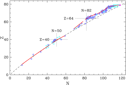
Figure 1: The path of the most probable atomic number $Z_{p}$ corresponding to the best fit values for the parameters $a_{6}-a_{8}$ in seven mass regions (solid lines). Positions of nuclei, for which a cumulative or an independent yield was determined, are denoted by circles and triangles, respectively. Dashed line - valley of stability approximated by the relation $Z_{\beta}=A/(1.98+0.0155A^{2/3})$ Marmier and Sheldon (1971). Open square indicates the target nucleus, vertical and horizontal dotted crosses are plotted for the magic $N=82$ and the closed shell $Z=64$ and for the magic $N=50$ and the closed shell $Z=40$.

As may be seen from Table 2, presenting the final parameters, sometimes the best fit is obtained when the number of parameters exceeds the number of data. This was done by fixing some parameters when the others were fitted, and vice versa. Various combinations and order of fixing/releasing of parameters as well as their total number were tested. The shape of the mass ridge could be parametrized with a maximum of four parameters, the most probable $Z$ path was approximated via a parabola except for two cases and the charge distribution width was constant or changed linearly with mass. Odd-even corrections were applied only for three heaviest mass regions, where a larger number of points and smaller relative errors of the experimental data allowed to get a reliable fit. The shape of the charge distributions was modeled better with the use of an asymmetric form for the evaporation residues, lying further from the stability valley (see Fig. 1). For lighter, fission products the $Z_{p}$ path goes closely along the valley of stability and here a symmetric Gaussian shape was more adequate.

Table 2: Best fit parameters obtained for the yield distribution model applied to six mass regions.

Paramater	Mass range
	163-182	150-161	143-149	121-139	82-103	24-75
$Y_{A}\quad a_{1}$	-93.98(2)	-90.63(3)	-479.2(1)	18.13(9)	-30.97(5)	-2.07(11)
$a_{2}$	1.0951(1)	1.060 (2)	6.486(1)	-0.207(1)	0.690(1)	-0.0059(18)
$a_{3}$	-0.00310(1)	-0.00302(2)	-0.02192(3)	-0.000706(5)	-0.00390(6)	0.00029(3)
$a_{4}$			-0.3(2)E-7	0.884(4)E-5
$Z_{p}$  $a_{6}$	96.26(4)	136.6(1)	-3.06(9)	-7.2(3)	-142.1(1)	0.77(10)
$a_{7}$	-0.6681(2)	-1.201(1)	0.5051(6)	0.525(3)	4.886(1)	0.456(2)
$a_{8}$	0.003081(1)	0.00485(5)	-0.000329(4)	-0.00029(2)	-0.0456(1)	-0.000329(2)
$a_{9}$				0.8(14)E-7	0.000153(1)
$\sigma$  $a_{10}$	-0.82(2)	1.17(4)	1.12(8)	0.91(9)	1.15(4)	2.12(11)
$a_{11}$	0.0105(2)					-0.013(2)
$F_{P}$  $a_{14}$	0.67(3)	0.82(5)	0.58(7)	1.	1.	1.
$a_{15}$	0.74(3)	0.91(6)	0.90(8)	1.	1.	1.
$w$  $a_{16}$	2.	2.	2.	2.	2.	2.
$a_{17}$	1.5	1.5	1.5	1.5	2.	2.
$\chi^{2}/NDF$	0.045	0.006	0.164	0.131	0.082	0.020

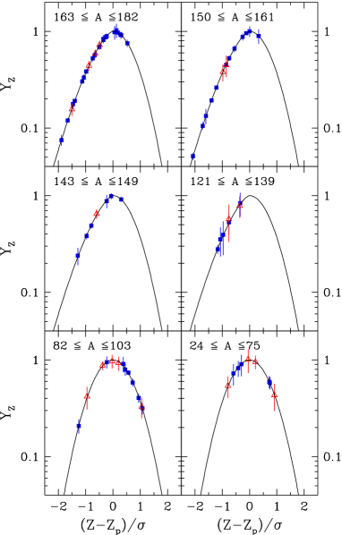
Figure 2: Normalized Z distributions for six mass ranges. The fitted function (line) is the exponent $\exp(-|(Z-Z_{p})/\sigma|^{w})$, where $w$ is the charge distribution power index, $Z_{p}$ the most probable $Z$ and $\sigma$ the Z distribution width. Experimental values ($\triangle$ - independent, $\blacksquare$ - cumulative) are normalized as described in the text. All distributions have the same normalized width equal to unity (please note the asymmetric shapes for four distributions of heavier isotopes, with different slope for both sides).

The normalized charge distributions for six mass intervals are plotted in Fig. 2 against the normalized charge difference $(Z-Z_{p})/\sigma$. This reduces the distributions to the same width in the case where $\sigma$ is not constant in the given region. The fitted function is the simple exponent $\exp(-|(Z-Z_{p})/\sigma|^{w})$, then, for comparison, experimental data $Y(A,Z)_{E}$ are normalized with three factors coming from the fit

$$Y_{Z}=\frac{Y(A,Z)_{E}}{Y(A)\times F_{P}(N,Z)\times f_{I}}.$$ (9)

Here, the mass distribution $Y(A)$ is as in Eq. (1), the odd-even correction $F_{P}(N,Z)$ follows Eq. (8) and the factor $f_{I}$ corresponds to the independent yield fraction in the case of the cumulative yield

$$f_{I}=\frac{\displaystyle F_{P}(Z,N)\int_{Z-0.5}^{Z+0.5}e^{-(z-Z_{p})^{w}/2\sigma^{2}}dz}{\displaystyle\sum_{k=0}^{5}\big{[}F_{P}(Z+ck,N-ck)\times\int_{Z+ck-0.5}^{Z+ck+0.5}e^{-(z+ck-Z_{p})^{w}/2\sigma^{2}}dz\big{]}}.$$ (10)

Sometimes charge distributions are normalized to unity integral over Z to get the total yield for a given A equal directly to $Y_{A}$ Sümmerer et al. (1990); Sihver et al. (1992). However, when odd-even corrections are used the distribution of the total yield cannot be described by a simple continuous function as in Eq. (2). Also the generalization of the charge distribution shape with the two-valued (or released) index $w$ leads to problems in obtaining an analytical form of the normalization factor for this function. Hence our distributions for six mass regions are normalized only to the same width $\sigma$ = 1, not to the same integral.

III.2 Treatment of the heaviest residues

It is a well known fact that none simple phenomenological model can properly describe the charge distribution of yields for isotopes lying near the target nuclide Silberberg and Tsao (1973); Sümmerer et al. (1990). The main reason for this is the asymmetric, non-Gaussian shape of the charge distribution, with the most probable $Z$ and width rapidly changing with mass. Such a phenomenon is clearly seen when one uses a longer section of the $Y(A,Z)$ yield, along constant $Z$ value instead of constant $A$. Fig. 3 presents isotopic $Y_{A}(A)$ distributions obtained in this experiment for elements ranging from Au to Lu. Also isotopic distributions obtained for the heaviest element after stopped antiproton absorption on ¹⁷⁶Yb, ¹⁴⁸Nd and ¹³⁰Te targets Lubiński (1997) exhibit such a behavior: a steep and narrow distribution for the target element $Z_{T}$, a flat and broad distribution for the $Z_{T}$-1 element and deformed quasi-Gaussian shapes for some smaller $Z$, with the deformation on the heavy mass side decreasing with increasing distance from $Z_{T}$. Even though the low mass side for all elements but $Z_{T}$ may be described with the same slope, the slope at the higher mass side changes rapidly and cannot be fitted well with a fixed isotopic distribution asymmetry, i.e. with the unique, constant $a_{17}$ parameter. As a consequence, the heaviest elements should be excluded from the global fit and their $Y_{A}(A)$ yields have to be fitted separately for a given $Z$.

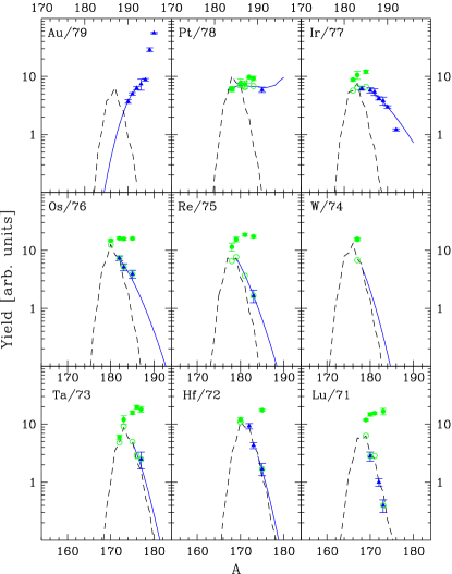
Figure 3: Isotopic yield distributions for the nine heaviest residual elements produced in the fragmentation of gold with stopped antiprotons. Dashed lines show yields obtained from the fit applied to the region $163\leq A\leq 182$; triangles, full and open circles represent the experimental yields: independent, cumulative and cumulative transformed to independent, respectively. Solid lines illustrate the corrections of the isotopic yield distribution for the heaviest isotopes of the elements from Pt to Hf, and for the lightest Au isotopes (see Sec. III for discussion).

The method of the yield completion for the heaviest elements is recursive: at the beginning we estimate the lacking yields of the lighter Au isotopes. With the use of these results cumulative, experimental yields for Pt are converted to independent ones and the isotopic distribution for this element is evaluated. Then, a similar procedure is applied for Ir, Os and so on. The method was applied down to Ta and Hf elements, where the yields for $A\geq 175$ were corrected. Finally, the summed $Y(A)$ yields for $A\geq 175$ presented with a line in Fig. 4 are the combination of results of both evaluations: the $163\leq A\leq 182$ region global fit and the procedure described above.

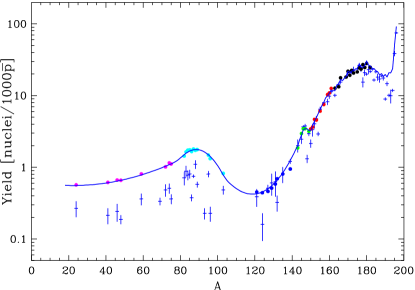
Figure 4: Mass distribution of residual nuclei produced by the reaction of stopped $\rm\overline{p}$ with Au. The cumulative sum of experimentally observed yields for a given mass is shown with crosses, the corresponding fitted $Y(A)$ yield for all input data (averaged over $Z$ for given $A$) is represented by full circles. The line shows the sum of fitted yields completed with interpolated yields for mass intervals not fitted. For the heaviest isotopes ($A\geq 175$) an additional correction of the mass yield data was performed, as described in Sec. III.

The platinum distribution was the most laborious case, due to lack of radioactive isotopes above mass 191 and owing to the strong odd-even $N$ effect (up to 30%), observed for this even-$Z$ element produced after low-energy absorption of antiprotons. The overall shape of the isotopic distribution was assumed to be similar to that observed for Tm residues after Yb fragmentation with antiprotons Lubiński (1997), with an increasing enhancement of yields for three heaviest nuclei, which for Pt are these with the mass numbers 194, 195 and 196. The number for ¹⁹⁶Pt obtained in this way ($16/1000\rm\overline{p}$) was confronted with the result of another estimation, based on the so-called halo factor dependence on separation energy $S_{n}$ of the neutron from target nucleus Lubiński et al. (1998). For heavy nuclei with $S_{n}$ close to 8 MeV the halo factor is of the order of $4\div 5$, hence, using the ¹⁹⁶Au yield the $Y(^{196}$Pt) should be between 14 and 23 per 1000$\rm\overline{p}$. These two estimations are consistent. For the lightest Pt isotopes we assumed that the steep slope coming from the $163\leq A\leq 182$ region fit is a good approximation, this assumption was used also for consecutive, lower $Z$ elements (we have checked the justification of this approach using the lightest mass data points of these isotopes in an additional test fit). At last, on the basis of observed changes of Pt yield for odd and even $N$ isotopes an appropriate correction was applied.

III.3 Region of the $\alpha$-decay

There is a narrow bump at $A$ = 147 in the mass yield distribution, a feature observed for Au Kaufman and Steinberg (1980); Michel et al. (1997) and for Ta Kozma et al. (1991); Gulda (1993) target fragmentation after reactions with protons, heavy ions and stopped antiprotons. The enhancement of the cross section in this region was suggested to be the result of $\alpha$-decay of nuclei above the $N$ = 82 shell Kaufman and Steinberg (1980), but the authors abstained to estimate quantitatively this effect due to lack of charge dispersion curves which could not be fitted for limited experimental data. We have done such an estimation for our data performing a preliminary fit for isotopes not affected by $\alpha$-decay, i.e. for $154\leq A\leq 161$, adding ¹⁵⁰Dy with an independent yield. Taking into account a charge dispersion yield $Y(A,Z)$ obtained in this way we have calculated appropriate decay corrections for experimentally measured yields of ¹⁵³Tb (+2.9% correction), ¹⁵³Gd (+2.8%), ¹⁵²Dy (+7.2%), ¹⁵²Tb (+6.0%), ¹⁵¹Tb (+14.8%), ¹⁵¹Gd (+13.6%), ¹⁵⁰Tb (+32.5%), ¹⁴⁹Gd (+5.5%), ¹⁴⁷Gd (-13.7%), ¹⁴⁷Eu (-12.1%) and ¹⁴⁶Gd (-23.7%). The experimental results listed in Table LABEL:yields are the corrected ones and were used for fitting in two mass ranges affected by this effect. As can be seen from Fig. 4 the corrections obtained are too small to remove the local yield maximum at $A$ = 147 (crosses show the yield before correction, circles after that). Therefore, $\alpha$-decay alone cannot explain fully such a feature and the observed yield enhancement in this region should be partially ascribed to the closed $N$ = 82 shell influence.

IV RESULTS

The experimental data are presented in Table LABEL:yields, together with the fit results for isotopes representing full yield for a given pair of $A$ and $Z$. Results are normalized to yield per 1000 $\rm\overline{p}$ with the total number of antiprotons stopped in the target ($9.25\times 10^{8})$. The final mass yield distribution is presented in Fig. 4. The cumulative sum of all yields observed for a given mass number $A$ is here compared with the total yield $Y(A)$ obtained from the fit via summation of all fitted $Y(A,Z)$ values over $Z$, or from the interpolation between fitted mass regions. The global curve of the fitted $Y(A)$ yield, when compared with the summed experimental yields, forms its exact skyline in almost the whole region of the evaporation residues. A deviation from this rule is observed for three mass ranges: the heaviest, with $A>176$, a few mass numbers around $A$ = 147 and all fission fragments ($A<120$). Except for the second region (affected by the $\alpha$-decay), this is the result of prevailing accumulation of the isobaric yield by non-detectable isotopes. The depression of observed yield of the heaviest evaporation residues is narrow but deep, with a maximum decrease to about 40% of the fitted $Y(A)$ for $A\approx 192$, and comes mainly from the stable Pt isotopes produced. For fission products, where the $Z_{p}$ path goes over the stability valley, the observed yield is strongly suppressed and its outline reaches only about 20-50% of the fitted yield.

Leaving out two heaviest masses, the maximal $Y(A)$ yield is reached at mass 180 but the largest individual $Y(A,Z)$ production is fitted for ¹⁷⁶W. The small yield peaks observed for some even masses ($A$ = 180, 176, 170, …) are due to the strongest odd-even effect for some even $Z$ lying almost on the $Z_{p}$ path. On the other hand, the global mass yield minimum appears between $A=105$ and $A=120$. As numerous $\gamma$-lines of strongly populated heavier nuclei covered this region, no valuable production limits can be given for this region and we have to stick to the interpolated curve.

After evaluation of the mass yield curve it is possible to estimate the relative yields for different reaction channels. The fission fragments mass range should be treated with some care as their multiplicity is equal to 2 or greater when one takes into account any multifragmentation process. Assuming that all residues with $40\leq A\leq 120$ are binary fission products (i.e. two heavy residues per antiproton) and neglecting the lightest $A<40$ masses, we have obtained the summed fission yield. Comparing this number with the total $Y(A)$ integral in the mass limits from 40 to 196 we have extracted the probability of gold fission induced with stopped antiprotons to be ($3.8\pm 0.5$)%. The lighter mass region ($A=10-40$), not taken into account in fission due to possible multiplicity $>2$ and/or the not fully negligible chance to have a fission partner in the $A>120$ region, constitutes additionally less than 0.9% of the total yield (the error quoted above takes this into account). Our result compares well with the fission probability of 3.1(3)% obtained in an experiment where fission fragments yields were measured with PIN diodes Schmid et al. (1994) and is substantially larger then the value of 1.5% derived from another experiment using also on-line technique Bocquet et al. (1992).

V DISCUSSION

V.1 Antiprotons versus other projectiles

The properties of reactions induced by stopped antiproton absorption can be investigated by comparison with yield distributions obtained for other, more ”classical” projectiles. We have confined this comparison to the gold target as the literature is quite rich here Kaufman and Steinberg (1980); Michel et al. (1997); Sümmerer et al. (1990); Sihver et al. (1992); Kaufman et al. (1976, 1979); Mustapha (1999). The two other popular neighbor-mass targets, Pb and Ta, represent rather different decay scenarios, with respectively more and less pronounced fission channel.

V.1.1 Mass yield curve

First, we present a rather qualitative comparison with the yield curve shapes extracted for protons. Figure 5 shows the summed isobaric $Y(A)$ yield obtained for stopped antiprotons plotted together with yield distributions resulting from Au fragmentation by 0.49, 0.8, 1.0 and 3.0 GeV protons Kaufman and Steinberg (1980); Rejmund et al. (2001); Benlliure et al. (2001). Since the yields for stopped antiprotons and protons are measured in different units, we have normalized our yield axis with an arbitrary factor equal to 0.57, providing the concordance between $\overline{p}$’s and 1 GeV protons results in the 150-170 mass range. It should be stated here that the yield curve presented for fission residues in the case of 1 GeV protons was fitted with only 5 mass points Kaufman and Steinberg (1980).

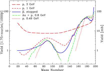
Figure 5: Comparison of the mass yield distribution obtained for protons and stopped antiprotons. Curves for protons at 0.49 GeV, 1.0 GeV and 3.0 GeV adopted from Kaufman and Steinberg (1980), for the inverse kinematic reaction of Au on H at 800 MeV from Rejmund et al. (2001); Benlliure et al. (2001). The yield axis for antiprotons was normalized with a factor of 1.75.

The most striking differences between the curves shown in Fig. 5 are seen for the fission region. The fission probability for gold excited by protons, estimated as in Sec. IV, is equal to $\approx$ 6.5%, $\approx$ 3.7% and $\approx$ 3.3% for 1 GeV, 0.8 GeV and 0.49 GeV protons, respectively. Then, 800 MeV protons seem to correspond to stopped antiprotons, but fission takes only a small part of the total yield and the comparison of distribution shapes in the evaporation region is much more adquate. Such inspection leads to the conclusion that stopped antiprotons match with protons at 1 GeV.

Besides the level and width of the fission hump, a second major feature distinguishing the mass yield shapes observed for stopped antiprotons and protons is the distribution for the heaviest masses close to the target. Here the experimental situation is much better than in the fission case: more reliable nuclear spectroscopy data is additionally confirmed by the results of inverse kinematic measurements. The yield distribution for protons is rather unchanged in energy range from 0.5 to 1 GeV and forms a plateau between $A\approx 175$ and $A\approx 194$. On the contrary, for antiprotons in this mass range, not only for the gold target Szmalc (1992); Gulda (1993); Lubiński (1997), the yield slowly decreases from $A\approx A_{T}-20$ to $A\approx(A_{T}-3)$ and then strongly rises, reaching an absolute maximum at $A=(A_{T}-1)$. The enhancement of yield for few masses closest to the target may be explained by two mechanisms. The first one is the soft antiproton absorption, where almost all annihilation pions miss the rest of the target nucleus. Then the $(A_{T}-1)$ nuclei are left with very low excitation energy. Only after antiproton absorption on nucleons occupying a deeper states Wycech et al. (1996) rearrangement of nucleon configurations results in a mass loss of one or two additional units. The probability of the production of ($A_{T}-1$) nuclei is quite large, about 10% for targets used in our nuclear periphery studies Lubiński et al. (1998); Schmidt et al. (1999) and the results obtained for gold are also of this order of magnitude (cf. Table LABEL:yields). The second mechanism leading to low excitation energies is the class of all processes where the annihilation pions escape unabsorbed by the target nucleus but due to the sizeable total $\pi$-nucleus cross section excite this nucleus enough to emit few nucleons. The probability of such kind of quasi-elastic meson escapes may be quite large when the nuclear diffuseness and partial opacity are considered Cugnon et al. (2001).

A quantitative comparison between antiprotons and other projectiles is presented in Table 3 and Fig. 6. For this purpose we have calculated the average mass removed from the target, $\Delta A$, defined as:

$$\Delta A=A_{T}^{\star}-\frac{\displaystyle\int_{A_{min}}^{A_{max}}Y(A)AdA}{\displaystyle\int_{A_{min}}^{A_{max}}Y(A)dA},$$ (11)

where $A_{T}^{\star}$ equals $A_{T}$ for protons and pions or $A_{T}-1$ for antiprotons. $A_{\rm min}$ is the lower integration limit adjusted to get all single heavy residues and $A_{\rm max}$ is equal to $A_{T}$ for protons and pions or to $A_{T}-2$ for antiprotons. The residual mass $A_{T}-1$ is ignored in the integration of the reaction yields for antiprotons since it attests no reaction (soft $\overline{p}$ absorption).

Table 3: Characteristics of the mass yield distribution after the reaction of different projectiles with a gold nuclei.

Projectile	$\rm Energy$	$\Delta A$	Ref.
	$\rm[GeV]$
$\pi^{+,-}$	$0.0$	$\phantom{1}7.2\pm 1.1$	Pruys et al. (1979)
$\pi^{+,-}$	$0.1$	$\phantom{1}8.7\pm 1.0$	Kaufman et al. (1979)
$\pi^{+,-}$	$0.18$	$10.4\pm 1.2$	Kaufman et al. (1979)
$\pi^{+,-}$	$0.3$	$12.2\pm 1.3$	Kaufman et al. (1979)
p	$0.2$	$\phantom{1}8.6\pm 1.1$	Kaufman and Steinberg (1980)
p	$0.49$	$14.9\pm 1.8$	Kaufman and Steinberg (1980)
p	$0.8$	$17.0\pm 1.4$	Mustapha (1999)
p	$0.76$	$17.8\pm 2.3$	Michel et al. (1997)
p	$0.8$	$18.0\pm 2.3$	Michel et al. (1997)
p	$1.0$	$20.7\pm 2.8$	Kaufman and Steinberg (1980)
p	$1.2$	$23.2\pm 3.2$	Michel et al. (1997)
p	$1.6$	$26.5\pm 3.4$	Michel et al. (1997)
p	$2.6$	$30.1\pm 1.9$	Sümmerer et al. (1990)
p	$3.0$	$30.6\pm 4.3$	Kaufman and Steinberg (1980)
p	$11.5$	$30.3\pm 4.2$	Kaufman et al. (1976)
p	$800.0$	$26.1\pm 3.7$	Sihver et al. (1992)
$\rm\overline{p}$	$0.0$	$17.3\pm 1.3$	von Egidy and Schmidt (1991)
$\rm\overline{p}$	$0.0$	$20.0\pm 0.8$	this work

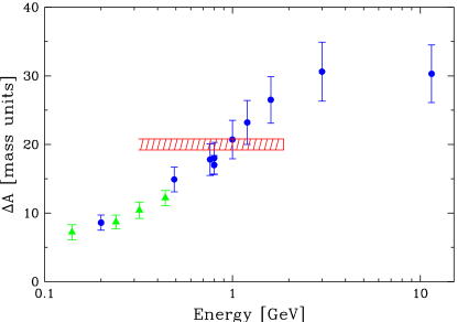
Figure 6: Average mass removal from the Au targets irradiated with: $\blacktriangle$, pions; $\bullet$, protons (Refs. cited in Table 3) and stopped antiprotons (pion data are shifted right by the $\pi$ rest mass). The hatched band shown for antiproton data reflects the error in $\Delta A$ and a possible range of energy deposition for stopped $\rm\overline{p}$ annihilation with one of the target nucleons.

To get consistent and comparable results, for each data set taken from the literature we have applied a uniform method to determine $\Delta A$. Only experimental data representing the highest (approximately the whole) cumulative yield for a given $A$ were used to construct the mass yield distribution curve. The absolute errors of the quantities presented in Table 3 were estimated to be of the order of 10-20%, but the relative errors should be smaller. In addition to proton data, results for pions absorbed by the gold target are presented, their energy range is limited as compared to the rest of data but coincides with the kinetic energy of pions emitted in antiproton annihilation. The average mass removal from the target nucleus smoothly correlates with the projectile energy. As can be seen from Table 3 and Fig. 6, the average mass removed from the gold target by stopped antiprotons is only slightly lower than $\Delta A$ obtained for 1 GeV protons.

V.1.2 Charge distribution

The information on the reaction mechanism, obtained from the investigation of mass yield distributions, may be enriched by the examination of other features of the $Y(A,Z)$ yield topography. Two such properties were compared for results of gold fragmentation by antiprotons and other projectiles: the course of the fitted $Z_{p}$ path and the charge dispersion width. Figure 7 illustrates such an inspection for some cases quoted in Table 3. To bring differences into prominence, we have recalculated $Z_{p}(A)$ to its distance $\delta_{stab}$ from the line modeling the beta stability valley $Z_{\beta}$ (defined as in the caption to Fig. 1). Such a presentation was earlier applied to study the distribution of products of gold projectile fragmentation on C and Al targets Souliotis et al. (1998). To compare with our results we present $\delta_{stab}$ obtained for the inverse kinematic Au + p reaction at 800 MeV Rejmund et al. (2001); Benlliure et al. (2001) and for energetic protons Kaufman et al. (1976); Kaufman and Steinberg (1980). Besides this, we have also plotted curves derived for the Au target from a general formulae describing the $Z_{p}(A)$ path for products of various medium and heavy target fragmentations induced with protons at the fragmentation limit Sümmerer et al. (1990) and with stopped antiprotons von Egidy and Schmidt (1991). The lower part of Fig. 7 shows the dependence of the charge distribution width on the product mass.

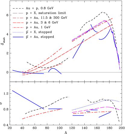
Figure 7: Upper part: Distance of the fitted most probable Z from the beta stability line: protons/heavy ions compilation at saturation limit Sümmerer et al. (1990), antiprotons at rest energy compilation von Egidy and Schmidt (1991), Au at 800 MeV on H Rejmund et al. (2001); Benlliure et al. (2001), protons at 11.5/300 GeV Kaufman et al. (1976), protons at 3/6 GeV Kaufman and Steinberg (1980) and fission for protons at 1 GeV Kaufman and Steinberg (1980). Lower part: Charge distribution widths as a function of residue mass. The results of the same evaluations as in the upper part are presented (with unchanged notation), except for protons at 1 GeV and at 3/6 GeV, for which the width parameter is equal to that obtained for 11.5/300 GeV Kaufman and Steinberg (1980).

As can be seen from Fig. 7, the relative course of $Z_{p}$ and $Z_{\beta}$ for stopped antiprotons changes now much more dramatically than in Fig. 1. The $\delta_{stab}$ calculated for more general $Y(A,Z)$ models Sümmerer et al. (1990); von Egidy and Schmidt (1991) is smooth due to the broad $A$ range fitting. $Z_{P}$ fitted for 11.5 and 300 GeV protons Kaufman et al. (1976) lies very close to this curves in the evaporation residues region. Surprisingly, $Z_{p}$ derived for the inverse reaction at smaller energy extends farther towards the neutron-deficient nuclei for heavy products. In the fission region the situation is reversed except for the lightest products. The curve plotted for 3 and 6 GeV protons lies closer to the valley of stability, for 1 GeV protons only the fission region is represented as there are no fit parameters given in Ref. Kaufman and Steinberg (1980).

When $Y(A,Z)$ models are applied to shorter mass ranges a rather non-continuous behavior with segments of rapidly changing position and orientation is observed. This happens both for protons Sihver et al. (1992) and heavy ions Kudo et al. (1984); Loveland et al. (1990a, b) investigated with $\gamma$-ray spectroscopy technique and for heavy ion reactions on Au studied with the inverse kinematic technique Souliotis et al. (1998). Obviously, this situation cannot be ascribed merely to the uncertainties of the experimental data, even in the worst cases. In our case, the experimental data distribution in the $N-Z$ plane shown in Fig. 1 strongly favors the segmentation of the evaporation region in fitting.

Generally, lower energy reactions lead to $Z_{p}$ running closer the valley of stability, with passages to the neutron-rich side for fission fragments. Antiproton data show a peculiar tendency: although $Z_{p}$ lies quite away from the valley of stability for evaporation residues, it does not reach such a neutron-deficient region as the energetic protons. Such a behavior may be partially explained by the influence of shell effects observed in antiproton distribution for $N/Z$ crossings at 106/76, 82/64 and 50/40. The $Y(A,Z)$ yield reaches local maxima in these regions, the most probable $Z$ goes towards the more neutron-deficient nuclei and the charge dispersion becomes broader, as can be seen from Fig. 7.

The width of the $Z$ distribution, $\sigma$, was found to decrease smoothly with decreasing $A$ when a generalized approach is used for protons Sümmerer et al. (1990) or antiprotons von Egidy and Schmidt (1991). On the contrary, results of fitting within shorter mass regions are again inconsistent with compilations using broad mass regions, with quite small widths for evaporation residues and with a large scatter of $\sigma$ for fission fragments Loveland et al. (1990a, b); Sihver et al. (1992). For antiprotons stopped in Au the charge width is rather small in the evaporation region, especially in comparison with 800 MeV/nucleon Au on H data. On the other hand, products of fission induced by stopped antiprotons are distributed quite broadly, similarly to the proton reaction products.

From a methodological point of view, results on $Z_{p}(A)$ and $\sigma(A)$ fitted in different ways are not consistent, even for protons at similar energies. The $Y(A,Z)$ modeling applied for wide mass regions may be reasonable for limited experimental data and for generalization purposes, however, this approach washes out any possible feature of more discrete nature. Hence, the division of input data to some $A$ subregions should work better in detailed studies, especially for lower excitation reactions.

V.2 Antiprotons stopped in various targets

There were many other targets irradiated with low energy antiprotons from LEAR Moser et al. (1989); von Egidy et al. (1990); Jastrzȩbski et al. (1993a); Szmalc (1992); Gulda (1993); Lubiński (1997). A review of some results of these experiments will allow us to look closer at antiproton induced reactions. Mass-charge yield models were fitted only for a part of these targets, the parameters of the mass yield distributions for the rest were evaluated on the basis of summed direct experimental $Y(A)$ yields. However, either for the former or the latter results, the yields for the heaviest nuclei, close to the target, are underestimated since a significant part of the total Y(A) is hidden in non-detectable isotopes. To take this effect into account, we recalculated $\Delta A$ values obtained for other targets in the way as it was done for Au (see Sec. V.1). The results are listed in Table 4. The removed mass increases with increasing target mass, as illustrated in Fig. 8. Such behavior is consistent with the simple geometrical picture of an excitation energy proportional to the number of participating nucleons Polster et al. (1995), hence to the volume of the nucleus bombarded with annihilation mesons.

Table 4: Characteristics of mass yield distribution after antiproton stopping in different targets.

Target	$\Delta A$	Ref.
natCu	$13.9\pm 1.8$	Jastrzȩbski et al. (1993a)
96Ru	$15.8\pm 1.9$	Lubiński (1997)
96Zr	$16.2\pm 2.0$	Lubiński (1997)
98Mo	$16.2\pm 2.1$	Moser et al. (1989)
106Cd	$16.4\pm 2.3$	Lubiński (1997)
natAg	$17.7\pm 1.8$	Szmalc (1992)
130Te	$18.9\pm 1.6$	Lubiński (1997)
natBa	$17.9\pm 2.1$	von Egidy et al. (1990)
144Sm	$17.5\pm 1.9$	Lubiński (1997)
148Nd	$19.4\pm 2.0$	Lubiński (1997)
160Gd	$19.2\pm 2.2$	Lubiński (1997)
165Ho	$21.7\pm 2.5$	Moser et al. (1989)
176Yb	$21.1\pm 2.0$	Lubiński (1997)
natTa	$22.4\pm 2.2$	Gulda (1993)
natAu	$20.0\pm 0.8$	this work

Using the $\Delta A$ value obtained for the Au target we may estimate the mean thermal excitation energy of the decaying system. The compilation of the measured particle emission Markiel et al. (1988); Hofmann et al. (1990); Polster et al. (1995) gives 5.4 nucleons ejected in the cascade+preequilibrium stages through n, p, d, t, ³He and ⁴He ejectiles. Hence we have on the average 14.6 evaporated nucleons and assuming 8 MeV separation energy and 3 MeV kinetic energy per nucleon Polster et al. (1995) leads to ($161\pm 23$) MeV stored in the thermalized system. Such a result compares nicely with the value of ($183\pm 21$) MeV derived from the measurements of the spectra of neutrons and of light charged particles Polster et al. (1995).

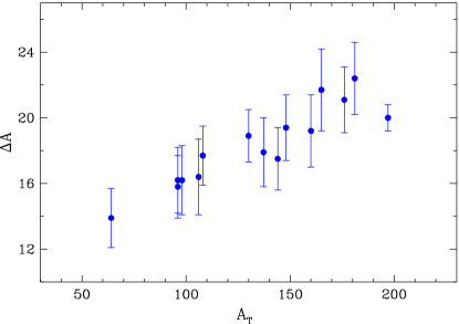
Figure 8: Average mass removed from different targets after stopped antiproton absorption. Results from earlier experiments studying mass yield curves Moser et al. (1989); von Egidy et al. (1990); Jastrzȩbski et al. (1993a); Szmalc (1992); Gulda (1993); Lubiński (1997), are recalculated after yield correction for the heaviest products.

V.3 Odd-even effects

Data on odd-even and shell effects observed in the $Y(A,Z)$ yield distribution are rather rarely discussed in the yield modeling context Rudstam (1966); Silberberg and Tsao (1973); von Egidy and Schmidt (1991). Their influence on the yields is difficult to observe if the experimental data set is limited and errors are of the order of the possible odd-even correction. The conclusion of Rudstam Rudstam (1966), looking for a general formula predicting cross sections for p and $\alpha$ induced reactions, was that there is no need to introduce such a correction as the experiment/model yield ratios for various N and Z combinations do not show any clear correlation with the nucleon number evenness. Later, Silberberg and Tsao Silberberg and Tsao (1973) found a moderate effect, modeled with factors equal to 1.25, 0.9, 1.0 and 0.85 for even-even, odd-N, odd-Z and odd-odd (N,Z) pairs, respectively.

Since off-line nuclear spectroscopy was applied to study the $Y(A,Z)$ distribution the odd-even effect was observed in reactions induced with stopped antiprotons Moser et al. (1989); von Egidy et al. (1990). Results for lighter targets (^92,95,98Mo, ^natBa) are consistent, with an 18-26 % correction for odd-Z nuclei and a 32-34 % correction for odd-N nuclei (and the sum of these values in the odd-odd case). Corresponding values fitted for ¹⁶⁵Ho Moser et al. (1989) are not so evident, the yield of odd-N nuclei is strongly reduced (by $\approx$ 66%) whereas there is no need to correct the odd-Z results. Because these fits were made simultaneously for the whole heavy residue region, no dependence on the emitted number of nucleons (hence excitation) was studied, also no indication for any shell effects was reported.

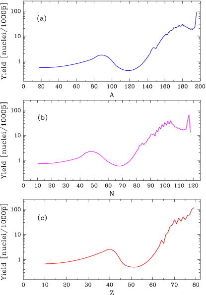
Figure 9: Yield of residues after gold fragmentation by stopped antiprotons: (a) as a function of the atomic mass A, (b) as a function of the neutron number N, (c) as a function of the atomic number Z.

Using the heavy and fissionable gold nuclei to absorb antiprotons we have the opportunity to investigate the odd-even and shell effects in a wide evaporation and fission products mass range. In Fig. 9 we present three fitted yield distributions, as function of mass, charge and neutron number of the products. Corrections fitted for odd-N and odd-Z yield were shown in Table 2 with parameters $a_{14}$ and $a_{15}$, respectively. They seem to be largest for the medium $\Delta A$ region ($161<A<182$), since between the heavier residues only the odd-N Pt isotopes exhibit a clear yield reduction of about 30%. A small odd-N effect ($\leq$ 10%) seems also to appear for the other heavy even-Z products. Lighter evaporation residues are produced more uniformly over changing nucleon numbers evenness, although for products close to the closed $N=82$ shell ($143<A<149$) the even-N isotopes are strongly favored. We have not been able to study odd-even effects for the lightest evaporation and all fission products because of their small cross sections with large relative uncertainties and since the experimental data are there much less numerous. It should be stated that the correction for odd-odd nuclei used here slightly differs from those applied before for stopped antiprotons Moser et al. (1989); von Egidy et al. (1990) as we use the multiplicative form (Eq. (3)) instead of a correction factor equal to $1-P_{n}-P_{p}$, where $P_{n}$ and $P_{p}$ are parameters fitted for odd-N and odd-Z nuclei, respectively. Since we observe that the odd-even effect is stronger when both $N$ and $Z$ are odd or even, the multiplication is more adequate.

The use of odd-even corrections for stopped antiproton reactions strongly improves the fit, with $\chi^{2}$ reduction by more than one order of magnitude. Thus it cannot be treated as a trivial improvement via adding another parameter. Moreover, since corrections obtained for different mass regions are consistent, therefore, taking into account previous results obtained for lighter targets Moser et al. (1989); von Egidy et al. (1990) the inclusion of such a component is unavoidable in correct modeling of the data coming from experiments with stopped antiprotons. Its strength, more pronounced than in the corresponding energetic proton data at 800 MeV Rejmund et al. (2001); Benlliure et al. (2001), is one of the most distinct features of the antiproton absorption induced reactions.

VI CONCLUSIONS

The independent and/or cumulative yields for 114 isotopes produced after absorption of stopped antiprotons in gold were measured by using the off-line $\gamma$-ray spectroscopy technique. On this basis, with the help of a phenomenological model, the whole yield distribution was extracted for residues ranging from the target mass minus one down to the light fission products with mass $\geq$ 20. The fission probability was estimated to be ($3.8\pm 0.5$)%, in agreement with the results of measurements using on-line techniques.

An average thermal excitation energy, gained by the Au nucleus after $\rm\overline{p}$ annihilation, was shown to be quite similar to that of 1 GeV protons, although the fission probability for such protons is almost twice as large. Moreover, the inspection of the yield distribution over the $A$-$Z$ plane indicates a fairly peculiar character of the reaction induced with low energy antiprotons. The most probable $Z$ course is quite different, lying closer to the stability line and exhibiting a more complex shape. Furthermore, the charge dispersion over $Z$ does not compare with that observed for 0.8 GeV protons, being almost twice as narrow.

The average mass removal observed for various targets reacting with stopped antiprotons rises linearly with increasing target mass. This behavior is consistent with in-beam studies of the light particle emission. $\Delta A$ derived from mass yield data helps to complete such measurements, unable to detect charged particles of the lowest energy.

A clear odd-even and some shell effects distinguish evidently the reaction with stopped antiproton from those induced with energetic protons. For the first time the dependence of this phenomenon on the residue mass was studied. The strength of such effects seems to diminish with the excitation energy, although for long evaporation chains and fission products it may be unobserved due to scarce and uncertain data.