Constructing the phase diagram of finite neutral nuclear matter

Abstract

The fragment yields from the multifragmentation of gold, lanthanum and krypton nuclei obtained by the EOS Collaboration are examined in terms of Fisher’s droplet formalism modified to account for Coulomb energy.  The critical exponents $\sigma$ and $\tau$ and the surface energy coefficient $c_{0}$ are obtained.  Estimates are made of the pressure-temperature and temperature-density coexistence curve of finite neutral nuclear matter as well as the location of the critical point.

I Introduction

In past attempts to investigate the relationship between nuclear multifragmentation and a liquid to vapor phase transition [1, 2, 3, 4, 5, 6, 7, 8, 9, 10, 11, 12] various studies have sought to determine one or more critical exponents [1, 3, 9, 10, 11, 13], other studies have examined caloric curves [4], and still others have reported the observation of negative heat capacities [8].  These studies suffer from the lack of knowledge of the system’s location in pressure-density-temperature $(p,\rho,T)$ space.  For example, interpretations of caloric curves and negative heat capacities depend on assumptions of either constant pressure or constant density [14, 15].  In the case of determining critical exponents, it was assumed that the fragmenting system is at coexistence and the dominant factor in fragment production was the surface energy.  The analysis presented below makes no assumptions about the location of the system in $(p,\rho,T)$ space and allows for other energetic considerations with regards to fragment production.

In this paper the analysis technique recently used on multifragmentation data collected by the ISiS Collaboration [10] is applied to the data sets for the multifragmentation of gold, lanthanum and krypton nuclei collected by the EOS Collaboration.  All three EOS experimental data sets are shown to contain the signature of a liquid to vapor phase transition manifested by the scaling behavior predicted by Fisher’s droplet formalism, and the liquid-vapor coexistence line is determined over a large temperature interval extending up to and including the critical point.  The critical exponents $\tau$ and $\sigma$, as well as the critical temperature $T_{c}$, the surface energy coefficient $c_{0}$ and the compressibility factor $C_{F}$ are directly extracted.  From the behavior of the fragment yields the $p$-$T$ and $T$-$\rho$ coexistence curves are determined and the critical pressure $p_{c}$ and critical density ${\rho}_{c}$ are estimated.

A Overview

The paper is organized as follows: section I B reviews the EOS data sets; section II A reviews Fisher’s droplet formalism and its connection to nuclear evaporation; section II B discusses the details of the data analysis; section II C reports the results of the data analysis; section II D shows the physical implications of these results; and finally, in section III a brief discussion of the results is made.  In order to demonstrate the efficacy of the analysis performed on the EOS data sets, an appendix shows the results of this analysis performed on percolation cluster distributions.

B EOS data sets

The EOS Collaboration has collected data for the reverse kinematics reactions $1.0$ AGeV Au$+$C, $1.0$ AGeV La$+$C and $1.0$ AGeV Kr$+$C [16, 17].  There were ${\sim}25,000$, ${\sim}22,000$ and ${\sim}36,000$ fully reconstructed events recorded for the Au$+$C, La$+$C and Kr$+$C reactions, respectively.  The term “fully reconstructed” means that the total measured charge in each event was within three units of the charge of the projectile.

FIG. 1.: (a) The distribution of events as a function of excitation energy.  (b) The nucleon number of the fragmenting system $A_{0}$ normalized to the nucleon number of the projectile $A_{\text{projectile}}$.  (c) The charge of the fragmenting system $Z_{0}$ normalized to the charge of the projectile $Z_{\text{projectile}}$.  (d) The number of intermediate mass fragments ($4\leq Z\leq Z_{0}/4$) $m_{\text{IMF}}$ normalized to the charge of the fragmenting system.  (e) The nucleon number of the largest fragment $A_{max}$ normalized to $A_{0}$.  (f) The charge of the largest fragment $Z_{max}$ normalized to $Z_{0}$.  (g) The multiplicity of fragments ($1\leq Z\leq Z_{max}$) resulting from the fragmentation of the system $m_{2}$ normalized to $Z_{0}$.

For every event, the charge and mass of the projectile remnant ($Z_{0}$, $A_{0}$) were determined by subtracting the charge and mass of the particles knocked out of the projectile from the charge and mass of the projectile [16, 17].

The thermal component of the excitation energy per nucleon of the remnant $E^{*}$ was determined as follows.  First, the total excitation energy per nucleon $E^{*}_{\text{total}}$ was reconstructed based on an energy balance between the initial stage of the excited remnant and the final stage of the noninteracting fragments.  The prescription [18] for calculating $E^{*}_{\text{total}}$ is then

$$E^{*}_{\text{total}}=\left[\sum\left(KE_{i}+Q_{i}\right)+\frac{3}{2}nT\right]/A_{0}$$ (1)

where $n$ is the multiplicity of neutrons produced via fragmentation, $KE_{i}$ is the kinetic energy of the $i^{\text{th}}$ fragment in the reference frame of the remnant and $Q_{i}$ is the removal energy and $T$ is the temperature of a Fermi gas.  For further details see reference [16].

The thermal component of the excitation energy per nucleon of the remnant $E^{*}$ was then determined by subtracting the expansion energy $E_{\text{X}}$ from $E^{*}_{\text{total}}$, where the quantity $E_{\text{X}}$ is given by

$$E_{\text{X}}=\left(\sum KE-E_{\text{th}}-E_{\text{Coulomb}}\right)/A_{0}$$ (2)

with $\sum KE$ the total kinetic energy; $E_{\text{th}}$ the sum of the translational thermal contribution to the fragment spectra; and $E_{\text{Coulomb}}$ the Coulomb contribution.

The translational energy is given by

$$E_{\text{th}}=\frac{3}{2}T_{\text{isotope}}(m_{2}+n-1)$$ (3)

where $m_{2}$ is the multiplicity of fragments and $T_{\text{isotope}}$ is the temperature calculated from the isotopic yields [16, 17].  This form follows that outlined in reference [19].

The Coulomb contribution is given by

$$E_{\text{Coulomb}}=\frac{3}{5}e^{2}\left[\frac{Z_{0}^{2}}{R_{r}}-\sum_{Z}\frac{N_{Z}Z^{2}}{(V_{r}/V_{0})^{1/3}R_{Z}}\right]$$ (4)

where $R_{r}$ is the radius of the excited remnant, $N_{Z}$ is the number of fragments with charge $Z$, $R_{Z}$ is the radius (at normal density) of a fragment with charge $Z$.  The volumes (and radii) were $V_{0}$ the volume of the remnant at normal density and $V_{r}=V_{\text{projectile}}(T_{\text{Fermi gas}}/T_{\text{isotope}})^{3/2}$ the volume of the excited remnant that isentropically expands from the normal volume of the projectile $V_{\text{projectile}}$ [16]; $R_{r}$ is then determined from $V_{r}$ assuming a spherical volume.  This form of $E_{\text{Coulomb}}$ follows reference [19] and takes into account the changing volume of the excited remnant as a function of excitation energy.  Previous estimates of $E_{\text{Coulomb}}$ did not account for the changing volume of the fragmenting remnant [16, 17].  This difference leads to a few AMeV difference in $E^{*}$ in the most violent collisions.

For the analysis in this paper, the data for each system was binned in terms of $E^{*}$ in units of $0.5$ AMeV; i.e. $20$ bins covered the excitation energy range $0\text{AMeV}\leq E^{*}\leq 10\text{AMeV}$.  Figure 1 shows some of the systematics of the EOS data binned in this manner.  These results are consistent with other EOS publications [12, 16, 17, 20].

The systematics of the EOS data sets shown in Fig. 1 demonstrates the similarity in behavior exhibited by the data sets when their differing sizes are taken into account by normalizing the quantity in question to the projectile charge $Z_{\text{projectile}}$ or the charge of the fragmenting system $Z_{0}$.  The exception is seen in Fig. 1d where only below $E^{*}\sim 4$ AMeV do all three systems behave similarly.  Above $E^{*}\sim 4$ AMeV, the size of the fragmenting systems dominate.  This is reflected in the ordering of $m_{\text{IMF}}/Z_{0}$; from lowest to highest: krypton, lanthanum and gold.

II Analysis

As with several other analyses [1, 3, 7, 8, 9, 10, 11, 21, 22, 23, 24], the basis of the present effort lies in an examination of the fragment yield distribution in the context of Fisher’s droplet formalism [25, 26, 27, 28, 29].  Thus, a brief review of Fisher’s formalism is given in the following section, together with a justification for its applicability to nuclear decay rates.

A Fisher’s droplet formalism

Fisher’s droplet formalism and its forerunners [30, 31] are based on an equilibrium description of physical clusters or droplets that condense in a low density vapor.  While Fisher’s formalism has long been applied to nuclear multifragmentation yields [1, 3, 7, 8, 9, 10, 11, 21, 22, 23, 24], the question arises as to the validity of a picture of clusters in equilibrium within a low density vapor to experiments in which excited nuclei undergo multifragmentation in vacuum.  Specifically: “In which sense is there an equilibrium between liquid and vapor in the free (vacuum) decay of a (multifragmenting) hot intermediate (nucleus)?”  Or more to the point: “Where is the vapor?”

If one assumes, as in a compound nucleus reaction, that the initial collision entity relaxes quickly to a hot thermalized blob, which proceeds slowly to emit particles stochastically, the answers to this question is simple.  The hot blob is the liquid which is evaporating in free space according to standard evaporation theories.  To establish coexistence, the vapor need not be present.  All that is necessary is to appreciate that:

1. in first order phase transitions the interaction between the two phases is unnecessary;

2. the rate of evaporation defines uniquely the vapor phase, even when the vapor phase is absent.

In fact the concentration of species $A$ is completely defined by

$$R_{A}=n_{A}(T)\overline{v_{A}}(T)$$ (5)

where $R_{A}(T)$ is the emission flux of $A$, $n_{A}(T)$ is the concentration of species $A$ and $\overline{v_{A}}(T)$ is the average velocity of $A$ which is of order of $\sqrt{T/A}$.  In other words, the outward flux, at equilibrium, is the same as the inward flux.

Thus a direct connection is made between the statistical decay rate and Fisher’s equilibrium description of cluster formation.  Two consequences follow:

1. At equilibrium, the evaporated particle is replaced by the back flux from the vapor.  However, since the back flux is absent in the case of nuclear multifragmentation, this analysis is limited to particles with low emission probability (first chance) and must avoid particles which are emitted with high multiplicity.  This is approximately achieved by eliminating fragments with $Z<4$ from the ensuing analysis.

2. In the same spirit as above, the pertinent temperature is that of the blob as it evaporates low probability particles.  Thus, rather than worrying about the role of high multiplicity particles and their associated cooling on the energy-temperature relationship, the Fermi gas relation ship $E=aT^{2}$ can be assumed with good confidence.

With this picture in mind, we return to Fisher’s formalism.

The basic idea is that in a non-ideal vapor of particles interacting with repulsive cores and short range attractive forces, can be approximated at low densities and temperature by an ideal gas consisting of noninteracting monomers, dimers, trimers at equilibrium.  The (free) energy of sufficiently large clusters can be estimated in terms of their volume and surface energy.  These clusters are in equilibrium with each other and the relative abundances of differently sized clusters changes with temperature and pressure [26].

The relative abundances of clusters with $A$ constituents is given by:

$$n_{A}=q_{0}A^{-\tau}\exp\left[-\frac{\Delta\mu A}{T}-\frac{c_{0}\varepsilon A^{\sigma}}{T}\right].$$ (6)

Here $q_{0}$ is a constant of proportionality which is fixed by the critical density [32, 33].  The power law $A^{-\tau}$ arises from a combinatorial factor that depends on the fact that the surface of the cluster must be closed [34, 35].  The distance from coexistence is:

$$\Delta\mu={\mu}_{l}-\mu,$$ (7)

where ${\mu}_{l}$ is the chemical potential the liquid at coexistence and $\mu$ is the chemical potential of the system.  For $\Delta\mu>0$ (a super-heated vapor) and $\Delta\mu=0$ (liquid-vapor coexistence) the above sum always converges.  While for $\Delta\mu<0$ (a super-saturated vapor), the sum diverges.  The “classical” part of the surface energy is parameterized by $c_{0}\varepsilon A^{\sigma}$, where $c_{0}$ is the zero temperature surface energy coefficient, $\varepsilon=(T_{c}-T)/T_{c}$ and $A^{\sigma}$ relates the number of constituents of a cluster to the most probable surface area.  Fisher’s critical exponents $\sigma$ and $\tau$ depend on the Euclidean dimensionality and universality class of the system.

The total pressure of the entire cluster distribution is given by summing all of the partial pressures $Tn_{A}$:

$$p={\sum}Tn_{A}$$ (8)

and the density is

$$\rho={\sum}An_{A}.$$ (9)

Thus the pressure and density of the system can be inferred from the knowledge of the cluster distributions.

At the critical point the system is at coexistence ($\Delta\mu=0$) and the classical part of the surface energy cost vanishes (${\varepsilon}=0$).  Thus both exponential factors are unity leaving only the temperature independent power law:

$$n_{A}=q_{0}A^{-\tau}.$$ (10)

Away from the critical point, but along the coexistence curve so that $\Delta\mu=0$, the cluster distribution is given by:

$$n_{A}=q_{0}A^{-\tau}\exp\left(-\frac{c_{0}\varepsilon A^{\sigma}}{T}\right).$$ (11)

Equation (11) can be rewritten as:

$$n_{A} = \left(q_{0}A^{-\tau}\exp\left(\frac{c_{0}A^{\sigma}}{T_{c}}\right)\right)\exp\left(-\frac{c_{0}A^{\sigma}}{T}\right)$$ (12)

$$= R\exp\left(-\frac{B}{T}\right).$$ (13)

Thus the cluster distribution along the coexistence curve is given by a Boltzmann factor with

$$R=q_{0}A^{-\tau}\exp\left(\frac{c_{0}A^{\sigma}}{T_{c}}\right)$$ (14)

and

$$B=c_{0}A^{\sigma}.$$ (15)

This Boltzmann factor manifests itself in Arrhenius plots for the fragment yields where a linear relation between $\ln(n_{A})$ and and $1/T$ is observed.  This behavior has long been observed in many nuclear fragment yield distributions [6, 36, 37, 38, 39, 40, 41] and has recently been observed in the cluster distributions of percolation (with the bond breaking probability playing the role of temperature) [36] and the Ising model [42].

As discussed above, Fisher’s formalism relates directly to a reaction rate picture.  In this picture, the heavy fragments (e.g. $Z\geq 4$) are the product of first chance emission from the excited remnant.  The first chance emission from a compound nucleus can be written as:

$$n_{A}(T)\propto\Gamma\propto e^{(-B/T)}.$$ (16)

Thus the fragment yields, parameterized via Fisher, can be related to the decay rates (widths $\Gamma$).  Furthermore, $\Gamma$, which controls the first chance emission yields, is the same decay width which controls the mean emission times $t$ since:

$$\Gamma t\approx\hbar,$$ (17)

thus

$$t\propto\frac{1}{\Gamma}\propto\frac{1}{n_{A}(T)}\propto e^{(B/T)}.$$ (18)

The mean time for fragment emission reported by the ISiS Collaboration [41, 43] is well described as a Boltzmann factor.  It was also noted that the Boltzmann factor describing the emission times is the same as that describing the fragment yields [44].  This indicates that the thermal reaction rate picture is valid for multifragmentation; fragments can be viewed as being the result of the evaporation of an excited nucleus.

B Fitting the data

Preliminary fits of the gold, lanthanum and krypton data with Eq. (6) led to puzzlingly large results for $\Delta\mu$ ($\left<\Delta\mu\right>\approx 3$ AMeV) which could be interpreted as a substantial degree of super-saturation.  A much more plausible alternative explanation is the lack of account of the Coulomb effects in Fisher’s formalism.  Equations (13) and (15) support the presence of a barrier controlling the flux from liquid to vapor and vice versa.  This barrier should depend not only on the surface energy of the fragment but should reflect the entire energy necessary to remove a fragment from the liquid and place it into the vapor.  At the least, the energy necessary to relocate a charge $Z$ from the bulk to “near” the surface of the “residual” nucleus should be evaluated.  This energy is negative and counteracts the effects of the surface energy.  Furthermore, it is to leading order, linear in $Z$ and thus in $A$.  Thus the large values of $\Delta\mu$.  An attempt to include the Coulomb energy explicitly is then

$$n_{A}=q_{0}A^{-\tau}\exp\left(\frac{A\Delta\mu+E_{Coul}}{T}-\frac{c_{0}\varepsilon A^{\sigma}}{T}\right).$$ (19)

with

$$E_{\text{Coul}}=\frac{\left(Z_{0}-Z\right)Z}{r_{0}\left(\left(A_{0}-A\right)^{1/3}+A^{1/3}\right)}\left(1-e^{-x\varepsilon}\right)$$ (20)

with $r_{0}=1.2$ fm.  In Eq. (20) there is a recognizable Coulomb interaction energy of two touching spheres modified by a factor $(1-\exp(-x\varepsilon))$.  The parameter $x$ (left as a fit parameter) takes into account the numerical coefficients of the linear term in $Z$ plus polarization effects, and $\varepsilon$ takes care of the need for the vanishing difference between the liquid and vapor near the critical point.  Note that the Coulomb energy discussed in Eq. (4) is different from the Coulomb energy discussed in Eq. (20).  Equation (4) describes the total Coulomb energy present in the fragmentation process, while Eq. (20) describes the cost in moving a fragment from the nuclear liquid to the nuclear vapor.

The mass of a fragment $A$ prior to secondary decay was estimated by multiplying the measured fragment charge $Z$ by $2$ and then by a factor of $(1+y(E^{*}/B_{f}))$ where $B_{f}$ is the binding energy of the fragment and $y$ is a fit parameter to allow for an increase or decrease in the amount of secondary decay.

The temperature was determined by assuming a degenerate Fermi gas,

$$T=\sqrt{\alpha E^{*}}.$$ (21)

The parameter $\alpha$ was taken to be [45]:

$$\alpha=8\left(1+\frac{E^{*}}{B_{0}}\right)$$ (22)

in order to accommodate the empirically observed change in $\alpha$ with excitation energy [46].  Here $B_{0}$ is the binding energy of the fragmenting system.  Using the Fermi gas approximation to relate $E^{*}$ and $T$ gives a reasonable estimate of the temperature of the excited remnant at the time of first chance emission.  It has been observed that even the isotope ratio thermometer follows the Fermi gas approximation quite well so long as the average number of IMFs is less than one [47].

To obtain the concentration of fragments of a given mass, the total number of fragments $N_{A}$ of a given size $A$ was normalized to the size of the fragmenting system $A_{0}$ so that $n_{A}=N_{A}/A_{0}$.

The location of the critical point, in terms of excitation energy, was determined from an examination of measured fluctuations.  In general, as the critical point of a system is approached from the two phase region, the difference between phases diminishes and the system fluctuates from one phase to the other.  At the critical point the fluctuations are maximal.  However, while the maximum in the fluctuations occurs at the critical point, the presence of a peak in the fluctuations is a necessary, but not sufficient, condition for a existence of a phase transition [9].

The fluctuations measured in the EOS data are: (1) in the charge of the largest fragment normalized to the charge of the fragmenting system, and (2) related to the average mass number of a fragment as measured by the quantity ${\gamma}_{2}$ [48], where

$${\gamma}_{2}=\left(\frac{\text{RMS}(A)}{\left<A\right>}\right)^{2}+1=\frac{M_{2}M_{0}}{M_{1}^{2}}$$ (23)

with $M_{k}$ as the $k^{\text{th}}$ moments of the fragment distributions

$$M_{k}=\sum_{A=1}n_{A}A^{k}.$$ (24)

These fluctuations are shown in Fig. 2.

The peak in the fluctuations was found by smoothing the data (solid lines in Fig. 2), taking the numerical derivative of the smoothed data and finding the value of $E^{*}$ where the the derivative passed through zero, see Fig. 3.  Finally, the value of the excitation energy at the critical point $E^{*}_{c}$ was determined by averaging the results from both measures of the fluctuations.  Table I lists the results.  For this analysis the values determined for the excitation energy at the critical point for the Au$+$C reaction are in proximity of other values observed in previous EOS analyses ($E^{*}_{c}\approx 4.75$ AMeV) [36, 16, 17].  Differences in the values of $E^{*}_{c}$ arise from the different method of constructing the thermal portion of the excitation energy described above [12, 20].

Estimates of the critical temperature $T_{c}$ are made by using the values of $E^{*}_{c}$ in Eq. (21) and lead to values, shown in Table I, that are comparable to theoretical estimates for small nuclear systems [49, 50, 51, 52].  As an aside, as shown in Table I the value of $T_{c}$ increases with decreasing projectile (and thus remnant) mass.  This is opposite of the trend assumed in a prior analysis of the EOS gold multifragmentation data where the Coulomb energy was neglected [9] but in agreement with the trend reported in other analysis of the EOS data sets [12, 20].

In Fig. 2 the value of ${\gamma}_{2}$ for the Kr system attains a peak value of only ${\sim}1.8$.  It has been suggested that the magnitude of the peak in ${\gamma}_{2}$ could distinguish between the presence of a power law with $\tau>2$ (${\gamma}_{2}>2$) and an exponential distribution (${\gamma}_{2}<2$) in the cluster yields [20, 48].  However, it was seen that this is not the case [9] and it will be seen in the Appendix that small percolation lattices have values of ${\gamma}_{2}$ with peak magnitudes of less than two yet still exhibit a continuous phase transition with an exponent of $\tau\sim 2.2$ in the power law describing the cluster yields at the critical point.  Thus, the height of the peak in ${\gamma}_{2}$ cannot be used to rule out the presence of a critical point and the associated power law in the cluster distribution or provide information about the value of the power law exponent.

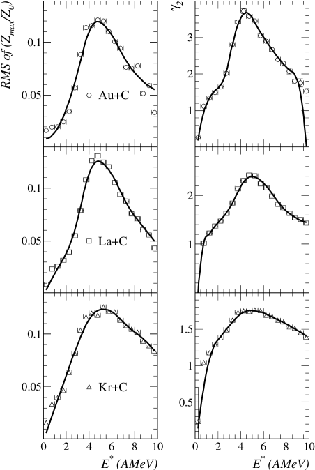
FIG. 2.: Left: The RMS fluctuations in the charge of the largest fragment normalized to the charge of the fragmenting system plotted as a function of excitation energy.  Right: The quantity ${\gamma}_{2}$ plotted as a function of the excitation energy.  Open symbols show the data points, solid curves show the results of smoothing the data.

FIG. 3.: Numerical derivatives of the smoothed data from Fig. 2 of: (left) the RMS fluctuations in the charge of the largest fragment normalized to the charge of the fragmenting system plotted as a function of excitation energy, and (right) the quantity ${\gamma}_{2}$ plotted as a function of the excitation energy.  Solid star symbols shows the approximate location in excitation energy where the derivative is zero, thus indicating the critical point.

TABLE I.: Critical points of excited nuclei

System	$E^{*}_{c}$ (AMeV)	$T_{c}$ (MeV)	${\rho}_{c}$ (${\rho}_{0}$)	$p_{c}$ (MeV$/$fm3)
Au $+$ C	$4.6\pm 0.2$	$7.6\pm 0.2$	$0.39\pm 0.01$	$0.11\pm 0.04$
La $+$ C	$4.9\pm 0.2$	$7.8\pm 0.2$	$0.39\pm 0.01$	$0.12\pm 0.04$
Kr $+$ C	$5.1\pm 0.2$	$8.1\pm 0.2$	$0.39\pm 0.01$	$0.12\pm 0.04$

Data from each system for $0.25$ AMeV $\leq E^{*}\leq E^{*}_{c}$ (which corresponds to a range of $0\leq\varepsilon<\sim 0.8$) and $4\leq Z\leq Z_{0}/4$ were simultaneously fit to Eq. (19), which, as mentioned previously, helps insure that the fragments examined in this analysis are produced via first chance emission.  There were nearly $200$ points from the EOS data sets used in the fitting procedure.  The fit parameters $\tau$, $\sigma$ and $c_{0}$ were kept the same for all three data sets while ${\Delta\mu}$, $x$ and $y$ were allowed to vary between the systems to minimize chi-squared; this gives $12$ free parameters used to fit nearly $200$ data points.  Previous analyses of the EOS data [9, 36] assumed that $\Delta\mu=0$ and that the effects of the Coulomb energy were small.  The analysis presented here makes no such assumptions.

Fixing $\tau$ at 2.2 did not significantly change the results of this analysis.  Using a common $x$ value for all three data sets also returned results similar to those quoted below.  Using a common $y$ value for all three data sets also returned results similar to those quoted below.   These different methods suggest a systematic error of $\sim 15$% of the value in question.  All errors quoted below are those returned by the fitting procedure, propagated where necessary.  Finally, the same data collapse observed below would be seen if the parameters were fixed to: $\tau=2.21$, $\sigma=0.64$ (their $d=3$ Ising values), $c_{0}=16.8$ MeV (the text book value of the nuclear liquid-drop surface energy coefficient), ${\Delta\mu}_{\text{Au,La,Kr}}=0$ (they must be close to zero since fragments are observed) and $y=0.5$ (in keeping with previous assumptions that the fragments prior to secondary decay have the same mass to charge ratio of the excited remnant [9, 12]) and letting only $x$, the Coulomb parameter vary to minimize chi-squared.

C Results

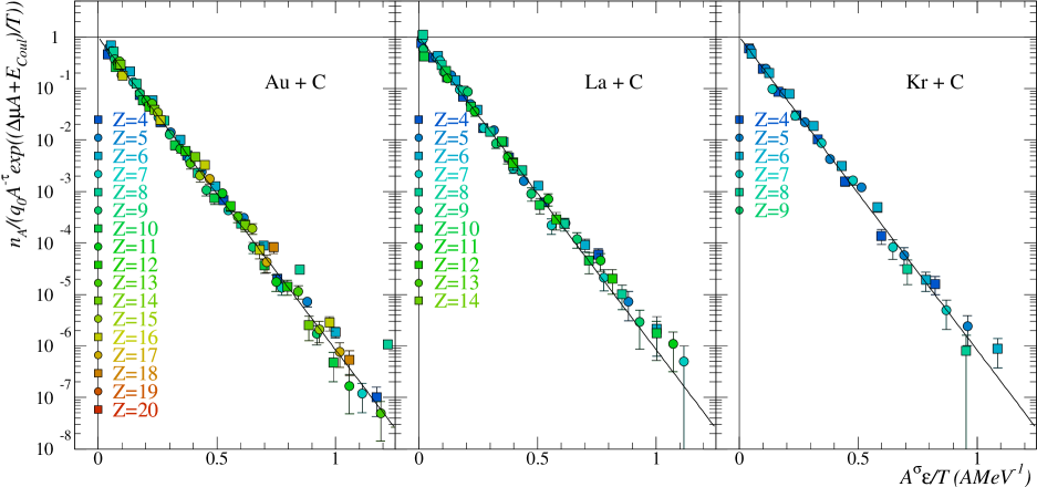
FIG. 4.: The scaled yield distribution versus the scaled temperature for the gold, lanthanum and krypton systems.  The solid line has a slope of $c_{0}$.

Figure 4 shows the fragment mass yield distribution scaled by the power law pre-factor, the chemical potential and Coulomb terms: $n_{A}/q_{0}A^{-\tau}\exp(({\Delta}{\mu}A+E_{\text{Coul}})/T)$ plotted against the inverse temperature scaled by Fisher’s parameterization of the surface energy: $A^{\sigma}\varepsilon/T$.  Now, the scaled data for all three systems collapse onto a single line over several orders of magnitude as predicted by Fisher’s droplet formalism [25].  This collapse provides direct evidence for a liquid to vapor phase transition in excited nuclei.  Furthermore, the fact that the data from each system show a common scaling illustrates the common nature of the underlying phenomenon.

1 Parameters

TABLE II.: Uncommon fit parameters

System	$\Delta\mu$ (AMeV)	$x$	$y$
Au $+$ C	$0.38\pm 0.02$	$1.1\pm 0.2$	$0.5\pm 0.1$
La $+$ C	$0.47\pm 0.03$	$1.2\pm 0.1$	$0.3\pm 0.2$
Kr $+$ C	$0.58\pm 0.08$	$4.0\pm 1.0$	$0.8\pm 0.2$

The values of $\tau=2.2\pm 0.1$, $\sigma=0.71\pm 0.02$ and $c_{0}=14.0\pm 1.0$ MeV determined in this analysis are in agreement with those determined for the ISiS gold multifragmentation data sets [10] and are in agreement with values previously determined for the EOS Au$+$C data set [12, 36].  The value of the surface energy coefficient $c_{0}$ is close to the value of the surface energy coefficient of the liquid-drop model which is $\sim 16.8$ MeV.

A previous analysis of the EOS gold multifragmentation showed the surface energy coefficient to be $c_{0}=6.8\pm 0.5$ MeV [36].  The difference between the $c_{0}=6.8\pm 0.5$ MeV from that work and the $c_{0}=14.0\pm 1.0$ MeV presented here arises from the differing analyses.  In the previous analysis it was assumed that $\Delta\mu=0$, that the Coulomb energy was negligible and that the level density parameter was constant at $\alpha=13$.  These assumptions allowed some degree of scaling, yielded sensible values for the critical exponents but resulted in a surface energy coefficient that was a factor of two of lower than that of the present analysis.

In addition to a surface energy coefficient that is in better agreement with the standard liquid-drop model, the greater collapse of the data in the present work demonstrates the improvements of the present analysis over the previous one.  The improvements in analysis are related to allowing a non-zero $\Delta\mu$, taking into account the cost in Coulomb energy to move a fragment from the liquid to the vapor and accounting for the change in the level density parameter over the excitation energy range.  The treatment of secondary decay in both analyses is different: previously it was assumed that the fragments, prior to any secondary decay, had the same mass to charge ratio as the fragmenting remnant.  In the present analysis the amount of secondary decay is left as a free parameter.

The values of $\Delta\mu$ reported in Table II can be considered “small” in light of Eq. (7).  The chemical potential of the liquid can be found by

$${\mu}_{l}=E_{0}+TS_{0}$$ (25)

with $E_{0}$ as the bulk energy per particle and $S_{0}$ as the bulk entropy per particle [25].  Treating the system as a Fermi gas so that $S/A=\alpha T$ yields

$${\mu}=E_{0}+E^{*}.$$ (26)

Thus the important energy scale for $\Delta\mu$ is $E_{0}+E^{*}$, for nuclear matter $E_{0}\sim 15.5MeV$.  The values of $\Delta\mu$ returned by this analysis are $<6$% of $E_{0}+E^{*}$ indicating the system is close to coexistence.  The values of $\Delta\mu$ should also be compared to the values returned when the EOS fragment yields were fit to (Eq. 6): $\left<\Delta\mu\right>\approx 3.0$ AMeV for all EOS reactions.  The reduction in the magnitude of the $\Delta\mu$ values is about a factor of six and is due to the modification of Eq. (6) to account for the Coulomb energy, i.e. Eq. (19).  The remaining small positive $\Delta\mu$ values of the systems may indicate that those systems are slightly super-saturated, or more probably they may reflect some other energy costs not taken into account (e.g. the symmetry energy or pairing), or they may reflect that the approximation for the cost in Coulomb energy to form a fragment given in Eq. (20) is not completely adequate (for instance Eq. (20) assumes a spherical geometry which may or may not be the case), or they may merely reflect noise in the data.

The values of $x$ for each system may indicate more (Au and La) or less (Kr) Coulomb energy present in the system.  They may also reflect the symmetry of the collision which may affect the geometry of the remnant, e.g. a very asymmetric collisions like Au$+$C may leave a nearly spherical remnant, while a more symmetric collision like Kr$+$C may result in a less spherical fragmenting system.

The values of $y$ returned indicate that the fragments have the same mass to charge ratio as the excited remnant.

The difference in values of $\Delta\mu$, $x$ and $y$ determined in the analysis of the three EOS data sets and those determined in the analysis of the ISiS $8.0$ GeV$/$c $\pi$ on gold multifragmentation set [10] is left an open question.  The small differences in $E^{*}_{c}$ and $T_{c}$ are due to the differences in reconstructed excitation energy scales [53].  This difference carries over to all energy related quantities, e.g. $c_{0}$.

Finally, in light of the above parameter results, it is clear that the same data collapse would be observed if the parameters were fixed to some nominal values, discussed above, with only $x$, the Coulomb parameter varying to minimize chi-squared.  Thus only three free parameters are truly needed to fit the $\sim 200$ data points of the EOS data sets.

D The coexistence curve of finite neutral nuclear matter

1 The pressure-temperature coexistence line

Before determining the pressure-temperature coexistence line, the meaning of a pressure associated with an excited nuclear remnant must be addressed.  As discussed above, in the actual experiment, this pressure is virtual; it is the pressure the vapor would have in order to provide the back flow needed to keep the source at equilibrium.  However, since the yields from Fisher’s formalism are proportional to both the pressure, Eq. (8), and the evaporation rate, Eq. (18), it is clear that by fitting the yields as has been done above, one can infer an associated (virtual) vapor pressure.

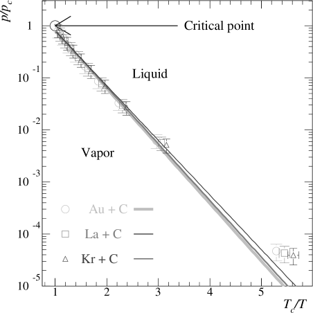
FIG. 5.: The reduced pressure-temperature phase diagram: the points show calculations performed at the excitation energies below the critical point and the lines show fits to the Clausius-Clapeyron equation.

The $p$-$T$ coexistence curve can be determined from this analysis.  As seen in section II A, Fisher’s theory assumes that the non-ideal fluid can be approximated by an ideal gas of clusters.  Accordingly, the quantity $n_{A}$ is proportional to the partial pressure of a fragment of mass $A$ and the total pressure due to all of the fragments is the sum of their partial pressures (see Eq. (8)).  The reduced pressure is then given by:

$$\frac{p}{p_{c}}=\frac{T\sum n_{A}(T)}{T_{c}\sum n_{A}(T_{c})}.$$ (27)

The coexistence curve for finite neutral nuclear matter is obtained by substituting the $n_{A}(T,\Delta\mu=0,E_{Coul}=0)$ from Eq. (19) in the numerator of Eq. (27) and $n_{A}(T_{c},\Delta\mu=0,E_{Coul}=0)$ in the denominator.  This allows one to transform the information in Fig. 4 into the familiar phase diagram in Fig. 5.  The data points shown give the values of $p/p_{c}$ and $T_{c}/T$ calculated via Eq. (27) for the bins in $E^{*}$ up to and including the critical point.

Figure 5 gives an estimate of the coexistence line of finite nuclear matter and from this it is possible to make an estimate of the bulk binding energy of nuclear matter.  One begins by assuming the system behaves as an ideal gas and uses the Clausius-Clapeyron equation

$$\frac{\partial p}{\partial T}=\frac{\Delta H}{T\Delta V}$$ (28)

where $\Delta H$ is the molar enthalpy of evaporation and $\Delta V$ is the molar volume difference between the two phases.   Then solving for the vapor pressure with

$$\Delta V=V_{\text{vapor}}-V_{\text{liquid}}\approx V_{\text{vapor}}=\frac{T}{p}$$ (29)

gives

$$p=p_{0}\exp(\frac{-\Delta H}{T})$$ (30)

which would lead to the ratio of

$$\frac{p}{p_{c}}=\exp\left[\frac{\Delta H}{T_{c}}\left(1-\frac{T_{c}}{T}\right)\right].$$ (31)

if $\Delta H$ were assumed to be temperature independent.  However, as $T\rightarrow T_{c}$ the gas is not ideal and $\Delta H\neq\text{constant}$, but it has long been known that for several normal fluids these deviations compensate so that $\ln(p/p_{c})$ is approximately linear in $T/T_{c}$ [54].

A fit of Eq. (31) to the coexistence curves for the systems is shown in Fig.5 yields the ratio of $\Delta H/T_{c}$.  Using the corresponding values of $T_{c}$ gives the molar enthalpies of evaporation of the liquid $\Delta H$ shown in Table III.  From these $\Delta H$ values $\Delta E$ is constructed via $\Delta E=\Delta H-pV$ with $pV=T$ (with the ideal gas approximation) using the average temperature from the range in Fig. 5 listed in Table III.  $\Delta E$ refers to the cost in energy to evaporate a single fragment.  To determine the energy cost on a per nucleon basis $\Delta E$ is divided by the most probable size of a fragment over the temperature range in Fig. 5.  Since the gas described by Fisher’s formalism is an ideal gas of clusters, the most probable cluster size is greater in size than a monomer.  The most probable size of a fragment in the region of the $p$-$T$ coexistence line obtained from Eq. (19) and the experimentally determined parameters is $1.05\pm 0.05$.  Thus the $\Delta E/A$ becomes $\approx$14 AMeV, close to the nuclear bulk energy coefficient of $15.5$ MeV.

TABLE III.: Thermodynamic properties of excited nuclei

System	$\Delta H$ (MeV)	$\left<T\right>$ (MeV)	$\Delta E/A$ (AMeV)	$C^{F}_{c}$
Au $+$ C	$19.4\pm 0.7$	$4.6\pm 0.6$	$14\pm 1$	$0.28\pm 0.09$
La $+$ C	$19.6\pm 0.7$	$4.9\pm 0.6$	$14\pm 1$	$0.28\pm 0.09$
Kr $+$ C	$19.5\pm 0.7$	$4.9\pm 0.6$	$14\pm 1$	$0.28\pm 0.09$

2 The temperature-density coexistence curve

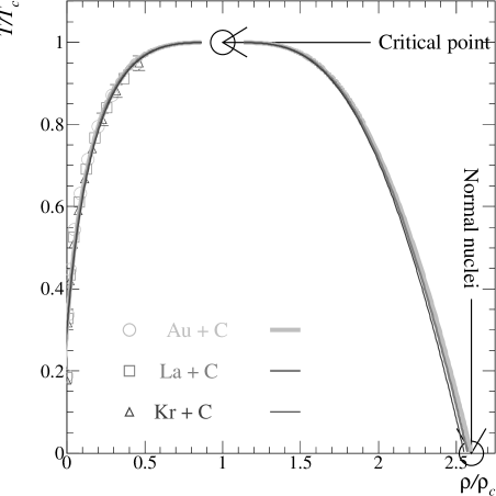
FIG. 6.: The points are calculations performed at the excitation energies below the critical point and the lines are a fit to and reflection of Guggenheim’s equation.

As seen in section II A the system’s density can be found from Eq. (9).  The reduced density is given by:

$$\frac{\rho}{{\rho}_{c}}=\frac{\sum An_{A}(T)}{\sum An_{A}(T_{c})}.$$ (32)

With $\Delta\mu$ and $E_{Coul}$ set to $0$ in the numerator of Eq. (19) and $\Delta\mu$ and $E_{Coul}$ set to $0$ with $T$ set to $T_{c}$ in the denominator, Eq. (32) gives the low density (vapor) branch of the coexistence curve of finite nuclear matter, shown in Fig. 6.

Following Guggenheim’s work with simple fluids, it is possible to determine the high density (liquid) branch as well: empirically, the $\rho/{\rho}_{c}$-$T/T_{c}$ coexistence curves of several fluids can be fit with the function [55]:

$$\frac{{\rho}_{l,v}}{{\rho}_{c}}=1+b_{1}(1-\frac{T}{T_{c}})\pm b_{2}(1-\frac{T}{T_{c}})^{\beta}$$ (33)

where the parameter $b_{2}$ is positive (negative) for the liquid ${\rho}_{l}$ (vapor ${\rho}_{v}$) branch.  Using Fisher’s formalism, $\beta$ can be determined from $\tau$ and $\sigma$ [25]:

$$\beta=\frac{\tau-2}{\sigma}.$$ (34)

For this work $\beta=0.3\pm 0.1$.  Using this value of $\beta$ and fitting the coexistence curve from the EOS data sets with Eq. (33) one obtains estimates of the ${\rho}_{v}$ branch of the coexistence curve and changing the sign of $b_{2}$ gives the ${\rho}_{l}$ branch, thus yielding the full $T$-$\rho$ coexistence curve of finite nuclear matter.

From Fig. 6 it is possible to make an estimate of the density at the critical point ${\rho}_{c}$.  Assuming that normal nuclei exist at the $T=0$ point of the ${\rho}_{l}$ branch of the coexistence curve, then using the parameterization of the coexistence curve in Eq. (33) gives ${\rho}_{c}\sim{\rho}_{0}/3$.  See Table I for precise values.

3 The pressure-density coexistence curve

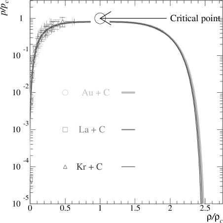
FIG. 7.: The points are calculations performed at the excitation energies below the critical point and the lines are the results of the fits from the previous sections.

For the sake of completeness the $p/p_{c}$-${\rho}/{\rho}_{c}$ projection of the coexistence curve is determined by combining the results of the previous two sections.  This is shown in Fig. 7.  It is clear from Fig. 7 that the fitted curves do not reach $p/p_{c}=1$ at ${\rho}/{\rho}_{c}=1$ while the data points do.  This is a reflection of the validity of the assumptions that went into deriving Eq. (31).

4 The compressibility factor

The critical compressibility factor $C^{F}_{c}=p_{c}/T_{c}{\rho}_{c}$ can also be determined in a straightforward manner from [28]:

$$C^{F}_{c}=\frac{\sum n_{A}(T_{c})}{\sum An_{A}(T_{c})}$$ (35)

Table III shows the results for the EOS data sets which are in agreement with the values for several fluids [28] and that of the ISiS data [10].

Finally, a measure of the pressure at the critical point $p_{c}$ can be made by using $T_{c}$ and ${\rho}_{c}$ from above in combination with $C^{F}_{c}$.  The results are shown in Table I.  This last calculation gives a complete experimental measure of the location of the critical point of finite neutral nuclear matter ($p_{c},T_{c},{\rho}_{c}$) and is in agreement with the ISiS results and in rough agreement with theoretical calculations [49, 52].

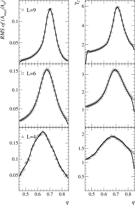
FIG. 8.: Left: The RMS fluctuations in the size of the largest cluster normalized to the size of the lattice system plotted as a function of bond breaking probability.  Right: The quantity ${\gamma}_{2}$ plotted as a function of bond breaking probability.  Open symbols show the estimate of the excitation at the critical point based on the maximum of the fluctuations, the solid line shows the results of smoothing the data.

FIG. 9.: Left: The numerical derivative of RMS fluctuations in the size of the largest cluster normalized to the size of the lattice system plotted as a function of bond breaking probability.  Right: The numerical derivative of the quantity ${\gamma}_{2}$ plotted as a function of bond breaking probability.  Open symbols show the estimate of the excitation at the critical point based on the maximum of the fluctuations, the solid stars show where the derivatives are zero.

III Conclusion

Through a direct examination of the most accessible features of nuclear multifragmentation, namely the fragment distributions themselves, and the use of Fisher’s droplet formalism, modified to account for the Coulomb energy cluster formation, a measurement of the coexistence curve of finite neutral nuclear matter has been made for three different multifragmenting systems and estimates of the critical point for finite nuclear matter have been made.  The precise values of quantities like the critical exponents and critical temperature and precise locations of coexistence curves depend on the assumptions made for the cost in Coulomb energy for fragment formation and the assumptions made to account for the secondary decay of the fragments.  While the exact forms are unknown, the estimates made in this paper have solid physical origins, and yield values of the surface energy coefficient and the bulk binding energy of nuclear matter which are consistent with established values.  Both the $p$-$T$ coexistence lines and the $T-\rho$ coexistence curves for all three EOS systems are consistent.  These are strong indications that this analysis determines the coexistence curve and can be used to construct the phase diagram of finite neutral nuclear matter based on experimental data.

IV Appendix

TABLE IV.: Critical points of finite percolation lattices

L	$q_{c}$	${\rho}_{c}$	$p_{c}$
$9$	$0.705\pm 0.004$	$0.210\pm 0.001$	$0.041\pm 0.001$
$6$	$0.685\pm 0.004$	$0.216\pm 0.001$	$0.041\pm 0.001$
$4$	$0.655\pm 0.004$	$0.243\pm 0.002$	$0.044\pm 0.001$

To demonstrate the efficacy of the above analysis, it is applied to the cluster distributions from three dimensional simple cubic lattices of side $L=4$, $6$ and $9$.  It will be seen that if the above procedures are followed, well known quantities are recovered.

Cluster distributions for over $100,000$ lattice realizations were generated by breaking bonds between sites [56].  A value of the lattice’s bond breaking probability $q$ was chosen from a uniform distribution on (0,1).  Next, a bond probability, $q_{i}$, was randomly chosen from a uniform distribution on (0,1) for the $i^{\text{th}}$ bond.  If $q_{i}$ was less than $q$, then the $i^{\text{th}}$ bond was broken and two sites were separated.  This process was performed for each bond in the lattice.  At low values of $q$, few bonds were broken resulting in a cluster distributions that are analogous to the liquid-vapor coexistence of a fluid.  In an infinite lattice the distinguishablity of the “liquid” phase and the “vapor” phase vanishes at a unique value of the lattice probability, $q_{c}$, when the probability of forming a percolating cluster changes from zero to unity [57, 58].  For the ensuing analysis, the number of clusters of size $A$ per lattice site $n_{A}$ was calculated by histogramming the lattice realizations into 100 bins on $q$ from $0$ to $1$.

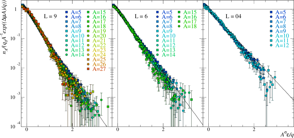
FIG. 10.: The scaled yield distribution versus the scaled bond breaking probability for the $L=9$, $6$ and $4$ lattices.  The solid lines has a slope of $c_{0}(L)$.

First the value of the probability at the critical point $q_{c}$ is determined by locating the maximum in the fluctuations of: (1) the size of the largest cluster, and (2) ${\gamma}_{2}$.  Figures 8 and 9 show these measures of the fluctuations.  The location of the maximum is determined as in the EOS data, the data is smoothed and then the numerical derivative is taken.  The location of the peak in the largest cluster is averaged with the location of the peak in ${\gamma}2$ and the results are recorded in Table IV.  As expected the value of $q_{c}$ changes with the lattice size.

Note that in Fig. 8 the value of ${\gamma}_{2}$ for the $L=4$ lattice attains a peak value of only ${\sim}1.9$; this is a finite size effect and due to the small size of the lattice.  Since ${\gamma}_{2}$ is related to the fluctuations in the average size of a cluster, it is clear that as the size of the lattice decreases, the upper limit in the size of a cluster decreases, thus imposing a limit on the size of ${\gamma}_{2}$.

TABLE V.: Percolation fit parameters

L	$\Delta\mu$	$c_{0}$
$9$	$-0.008\pm 0.004$	$2.62\pm 0.04$
$6$	$0.001\pm 0.001$	$2.42\pm 0.04$
$4$	$0.007\pm 0.001$	$1.91\pm 0.04$

Next the cluster yields from the three different lattices are fit simultaneously to Eq. (6), with $q_{c}(L)$ keeping the fit parameters $\sigma$ and $\tau$ consistent between lattices and letting $\Delta\mu$ and $c_{0}$ vary between lattices.  Data from $0.4\leq q\leq 1.05q_{c}$ and $5\leq A\leq 3L$ were included in the fitting procedure.  This gives seven fit parameters with $1083$ points to fit.  The results are shown in Fig. 10 and recorded in Table V.

The formula in Eq. (6) used in this analysis is only one example of a more general form of the scaling assumption [57, 58]

$$n_{A}=A^{-\tau}f\left(X\right)$$ (36)

with $X=A^{\sigma}{\varepsilon}^{\varphi}/T$ and where $f(X)$ is some general scaling function.  This scaling function should be valid on both sides of the critical point.  For small $X$ ($T\approx T_{c}$ and small $A$) and $\varepsilon>0$, $f(X)$ will vary as $\exp(-X)$ with $\sigma=1/(\beta\delta)=1/(\gamma+\beta)=0.64$ for $d=3$ Ising systems or $0.45$ for $d=3$ percolation systems and $\varphi=1$.  For large $X$ ($T$ far from $T_{c}$ or large $A$) and $\varepsilon>0$, $f(X)$ will vary as $\exp(-X)$ with $\sigma=2/3$ for all three dimensional systems and with $\varphi=2\nu$; where $\nu=0.63$ for $d=3$ Ising systems and $\nu=0.88$ for $d=3$ percolation lattices.

The fitting procedure using Eq. (6) returned a value of $\sigma=0.44\pm 0.01$ and $\tau=2.192\pm 0.003$ in good agreement with other measurements, $\sigma=0.45$ and $\tau=2.18$ [58].  It is clear from these results that the data examined here is in the small $X$, $\varepsilon>0$ region where the approximation of $f(X)$ given in Eq. (6) is valid.  As with the EOS data, the errors quoted here are from the fitting procedure.  Systematic errors that arise from the use of Fisher’s scaling form and from the fitting regions in $A$ and $q$ are on the order of $\sim 10$%.

The value of $c_{0}$ for the $L=6$ lattice is in good agreement with previous measures [36].  The interpretation of the change in $c_{0}$ with lattice size will be discussed below.

The values of $\Delta\mu$ for all lattices are close to zero, in agreement with the fact that percolation calculations such as these are at coexistence.

It is now a simple matter to follow the analysis described above using Fisher’s parameterization of the cluster distribution to determine the “phase diagrams” for these percolation lattices.  The interpretation of these “phase diagrams” is not as simple.

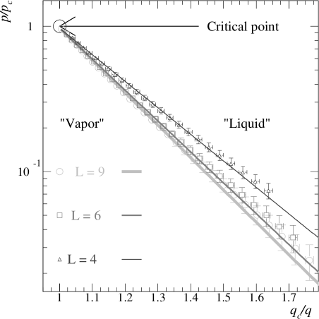
FIG. 11.: The reduced pressure-probability phase diagram: the points show calculations performed at the probabilities below the critical point and the lines show fits to the Clausius-Clapeyron equation.

First the “reduced pressure” as a function of the inverse of the “reduced probability” $q/q_{c}$ is determined via Eq. (27), and as usual for percolation studies $q$ replaces $T$ and $q_{c}$ replaces $T_{c}$.  The results are shown in Fig. 11 where the points are fit with Eq (31).  This leads to an estimate of the “enthalpy of evaporation of a cluster” given in Table VI.  The values of $\Delta H$ are on the order of the values of $c_{0}$ and increase with increasing $L$.

TABLE VI.: “Thermodynamic” properties of finite percolation lattices

$L$	$\Delta H$	$\Delta E/A$	$C^{F}_{c}$	bonds$/$site
$9$	$3.62\pm 0.03$	$2.7\pm 0.1$	$0.275\pm 0.003$	$2.67$
$6$	$3.35\pm 0.03$	$2.2\pm 0.1$	$0.275\pm 0.003$	$2.50$
$4$	$2.75\pm 0.03$	$1.8\pm 0.1$	$0.275\pm 0.003$	$2.25$

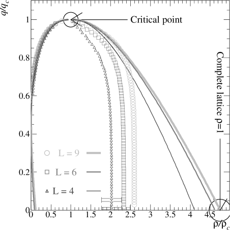
FIG. 12.: The points shown on the low density branch are from the calculations performed at the bond breaking probabilities below the critical point.  The lines are a fit to and reflection of Guggenheim’s equation.  The points shown on the high density branch show the size of the largest fragment at a given value of $q$ normalized to the size of the largest fragment at $q_{c}$.

To determine the “energy of vaporization” of a cluster $\Delta E$ the ideal gas approximation $pV=q$ is followed so that $\Delta E=\Delta H-q$, where $T$ is replaced by $q$ in keeping with standard practice in percolation work and $q$ is the average bond breaking probability considered; $0.56\pm 0.02$, $0.54\pm 0.02$ and $0.53\pm 0.02$ for $L=9$, $6$ and $4$ respectively.  The $\Delta E/A$ values listed in Table VI were found by dividing $\Delta H-q$ by the most probable cluster size ($1.15\pm 0.05$, $1.25\pm 0.05$ and $1.25\pm 0.05$ for $L=9$, $6$ and $4$ respectively), this puts $\Delta E$ on a “per site” basis.

The values of $\Delta E/A$ shown in Table VI are nearly identical to the values of the surface energy coefficient $c_{0}$, which is not surprising since for percolation on a simple cubic lattice $c_{0}$ arises from the bonds broken to form the surface.  Furthermore, the “energy of vaporization” is approximately equal to the number of bonds per lattice site (also shown in Table VI), a strong indication that the $\Delta E/A$ calculated here is the “bulk binding energy” of the lattice in question.  The value of $\Delta E/A$ decreases with the size of the lattice because the percolation calculations were performed for open boundary conditions.

The compressibility factor at the critical point was determined via Eq. (35), the results are shown in Table VI.  From $C^{F}_{c}$, $q_{c}$ and ${\rho}_{c}$ (determined below) the “pressure” at the critical point can be found.  The resulting values of $p_{c}$ are shown in Table IV, but the interpretation of these values is an open question.

Following the thermodynamic treatment of the percolation results, the reduced probability versus “reduced density” phase diagram is produced via Eq. (32).  This leads to the points shown in Fig. 12.  These points are then fit to Guggenheim’s empirical formula, Eq. (33), with $\beta=0.43\pm 0.01$ (in good agreement with text book values $0.41$ [58]) from Eq. (34).  These results are shown for each lattice by the solid lines in Fig. 12.

While it is not clear what density this plot describes, some insight can be gained by noting that the “liquid” branch reaches ${\rho}/{\rho}_{c}\sim 4$ to $\sim 4.5$ at $q=0$.  Assuming that at $q=0$ $\rho=1$, since no bonds are broken, then ${\rho}_{c}\sim 0.22$ to $\sim 0.25$, which is approximately the percentage of bonds broken at the critical point.  Thus it seems that the density in Fig. 12 is related to the number of broken bonds.  It is also noted that for $q=0$ the vapor branch of the coexistence curve shows ${\rho}/{\rho}_{c}>0$, this serves as an illustration of the magnitude of the error associated with this procedure.

It is also possible to directly explore the behavior of the reduced density of the “liquid,” at least in the larger system.  This is done by normalizing the size of the largest cluster at a given value of $q$ to the size of the largest cluster at the critical point $A_{\text{max}}(q)/A_{\text{max}}(q_{c})$.  Figure 12 shows that for the $L=9$ lattice, the measured normalized density of the liquid tracks along the coexistence curve predicted by Guggenheim’s empirical formula and the reduced density of the vapor.  For $q/q_{c}<0.75$ the effects of the finite size of the lattice are observed and the measured reduced density of the liquid deviates from the coexistence curve.  The effects of finite size are more evident in the smaller lattices where there is little or no agreement between the measured reduced density of the liquid and the coexistence curves.  Effects of finite size on the largest cluster such as these have been observed previously [59].

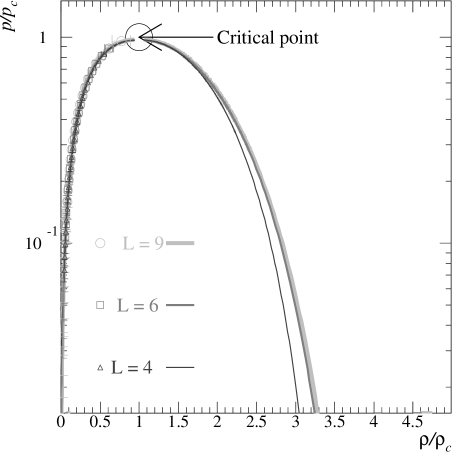
FIG. 13.: The points are calculations performed at the bond breaking probabilities below the critical point and the lines are the results of the fits from the previous sections.

For the sake of completeness, the “reduced pressure” versus “reduced density” projection of the phase diagram is shown in Fig. 13.

REFERENCES

- [1] J. E. Finn et al., Phys. Rev. Lett. 49, 1321 (1982).
- [2] P. J. Siemens, Nature 305, 410 (1983).
- [3] M. L. Gilkes et al., Phys. Rev. Lett. 73, 1590 (1994).
- [4] J. Pochodzalla et al., Phys. Rev. Lett. 75, 1040 (1995).
- [5] X. Campi and H. Krivine, Nucl. Phys. A 620, 46 (1997).
- [6] L. G. Moretto et al., Phys. Rep. 287, 249 (1997).
- [7] A. Bonasera et al., La Rivista Del Nuovo Cimento 23, 1 (2000).
- [8] M. D’Agostino et al., Phys. Lett. B 473, 219 (2000).
- [9] J. B. Elliott et al., Phys. Rev. C 62, 064603 (2000).
- [10] J. B. Elliott et al., Phys. Rev. Lett. 88, 042701 (2002).
- [11] M. Kleine Berkenbusch et al., Phys. Rev. Lett. 88, 022701 (2002).
- [12] B. K. Srivastava, et al., nucl-ex/0202023v1 (2002).
- [13] M. D’Agostino et al., Nucl. Phys. A 650, 328 (1999).
- [14] L. G. Moretto et al., Phys. Rev. Lett. 76, 2282 (1996).
- [15] J. B. Elliott and A. S. Hirsch, Phys. Rev. C 61 054605 (2000).
- [16] J. A. Hauger et al., Phys. Rev. C 57, 764 (1998)
- [17] J. A. Hauger et al., Phys. Rev. C 62, 024626 (2000).
- [18] D. Cussol et al., Nucl. Phys. A561, 298 (1993).
- [19] J. P. Bondorf et al., Phys. Rep. 257, 133 (1995).
- [20] B. K. Srivastava, et al., Phys. Rev. C 64, 041605(R) (2001).
- [21] A. S. Hirsch et al., Phys. Rev. C 29, 508 (1984).
- [22] A. L. Goodman et al., Phys. Rev. C 30, 851 (1984).
- [23] M. Mahi et al., Phys. Rev. Lett. 60, 1936 (1988).
- [24] X. Campi, Nucl. Phys. A 495, 259 (1989).
- [25] M. E. Fisher, Physics 3, 255 (1967).
- [26] M. E. Fisher, Rep. Prog. Phys. 30, 615 (1969).
- [27] C. S. Kiang and D. Stauffer, Z. Physik 235, 130 (1970).
- [28] C. S. Kiang, Phys. Rev. Lett. 24, 47 (1970).
- [29] D. Stauffer and C. S. Kiang, Advances in Colloid and Interface Science 7, 103 (1977).
- [30] J. E. Mayer and M. G. Mayer, “Statistical Mechanics”, John Wiley, New York (1940).
- [31] J. Frenkel, “Kinetic Theory of Liquids”, Oxford University Press (1946).
- [32] K. Binder and H. Müller-Krumbhaar, Phys. Rev. B, 9, 2328 (1974).
- [33] H. Nakanishi and H. E. Stanley, Phys. Rev. B 22, 2466 (1980).
- [34] M. E. Fisher and M. F. Sykes, Phys. Rev. 114, 45 (1959).
- [35] J. W. Essam and M. E. Fisher, J. Chem. Phys. 38, 802 (1963).
- [36] J. B. Elliott et al., Phys. Rev. Lett. 85, 1194 (2000).
- [37] K. Tso et al., Phys. Lett. B 361 (1995).
- [38] L. Phair et al., Phys. Rev. Lett. 77, 822 (1996).
- [39] L. Beaulieu et al., Phys. Rev. Lett. 81, 770 (1998).
- [40] L. G. Moretto et al., Phys. Rev. C 60, 031601 (1999).
- [41] L. Beaulieu et al., Phys. Rev. C 63, 031302 (2001).
- [42] C.M. Mader et al., LBNL-47575, nucl-th/0103030 (2001).
- [43] L. Beaulieu et al., Phys. Rev. Lett. 84, 5971 (2000).
- [44] L. Phair et al., LBNL-50069, contributions to the proceedings of the XIth International Winter Meeting on Nuclear Physics, Bormio, Italy (2002).
- [45] A.H. Raduta et al., Phys. Rev. C 55, 1344 (1997).
- [46] K. Hagel et al., Nucl. Phys. A486, 429 (1988).
- [47] J. B. Natowitz et al., nucl-ex/0106016v2 (2001).
- [48] X. Campi, Phys. Lett. B 208, 351 (1988).
- [49] H. R.Jaqaman et al., Phys. Rev. C 27, 2782 (1983).
- [50] H. R. Jaqaman et al., Phys. Rev. C 29 (1984).
- [51] P. Bonche et al., Nucl. Phys. A 436, 265 (1985).
- [52] J. N. De et al., Phys. Rev. C 59, R1 (1999).
- [53] T. Lefort et al., Phys. Rev. Lett. 83, 4033 (1999).
- [54] E.A. Guggenheim, “Thermodynamics”, th ed. (North-Holland, 1993).
- [55] E. A. Guggenheim, J. Chem. Phys., 13, 253 (1945).
- [56] J. B. Elliott et al., Phys. Rev. C 55, 1319 (1997).
- [57] D. Stauffer, Phys. Rep. 54. 1 (1979).
- [58] D. Stauffer and A. Aharony, “Introduction to Percolation Theory”, 2nd ed. (Taylor and Francis, London, 2001).
- [59] J. B. Elliott et al., Phys. Rev. C 49, 3185 (1994).