Multifragmentation process for different mass asymmetry in the entrance channel around the Fermi energy

Abstract

The influence of the entrance channel mass asymmetry upon the fragmentation process is addressed by studying heavy-ion induced reactions around the Fermi energy. The data have been recorded with the INDRA $4\pi$ array. An event selection method called the Principal Component Analysis is presented and discussed. It is applied for the selection of central events and furthermore to multifragmentation of single source events. The selected subsets of data are compared to the Statistical Multifragmentation Model (SMM) to check the equilibrium hypothesis and get the source characteristics. Experimental comparisons show the evidence of a decoupling between thermal and compressional (radial flow) component of the excitation energy stored in such nuclear systems.

1 Introduction

The characterization of the equation of state of nuclear matter can be carried out by the study of the fragmentation process in heavy-ion induced reactions [1, 2, 3]. In the Fermi energy range, the interplay between the attractive mean-field interaction and the individual nucleon-nucleon scattering is reached and the time scales of the collision become comparable to the deexcitation times [4]. In this case, one could expect to observe some deviations to the simplistic scenario consisting in the formation and de-excitation of a hot and equilibrated nucleus and the role of the dynamics of the collision could then be probed and quantified. The multifragmentation process, occuring in very dissipative reactions and successfully described as a statistical process [5], can be studied in order to shed light on this issue.

In this work, we have isolated and studied the characteristics of multifragmentation samples of central events for the ⁵⁸Ni + ¹⁹⁷Au system, ranging from $32A$ to $90A$MeV, and for the ${}^{129}Xe+^{nat}Sn$ system at $50A$ MeV, both registered with the INDRA $4\pi$ array. Both theoretical and experimental comparisons were performed and have allowed to address the issue of the fragmentation process and its relationship to the dynamics of the collision. The article is organised as follows. The second section presents the experimental details about the studied systems. The third section is devoted to the presentation of a new event selection method of the most violent collisions (called central collisions hereafter for the sake of simplicity). This method will allow us to carefully isolate in a second stage multifragmentation event samples. The gross features of the selected events is presented in the fourth section and the comparison protocol is detailed. The fifth section presents the comparison of the selected samples with a statistical model (SMM) in order to evaluate their degree of equilibration and will discuss in what extent a statistical approach can account for the deexcitation process. At last, the sixth section compares systems with different entrance channel characteristics (mass asymmetry and incident energy), in order to give an experimental answer to the question of the influence of the dynamics upon the deexcitation process of hot composite systems formed in heavy-ion induced reactions in the Fermi energy domain.

2 Experimental details

The Nickel beam was accelerated through the two coupled-cyclotrons at $74A$ and $90A$ MeV and then degraded in order to cover the incident energy range between $32A$ and $90A$ MeV. The beam intensity was below $10^{8}$ ion/s in order to keep the random coincidences as low as possible ($<10^{-4}$). The projectiles were impiged on a $200\mu g/cm^{2}$ self-supported $Au$ target. The experimental setup was constituted by the INDRA $4\pi$ array [6]. It is composed by $336$ two- or three-layers telescopes, depending on the polar angle, disposed in a cylindrical geometry along the beam direction into $17$ rings from $2$ to $176^{o}$ covering $90\%$ of $4\pi$. The first ring ($2<\theta<3^{o}$) was made of $12$ phoswich plastic scintillators ($NE115$/$NE102$). The forward part (from $3$ to $45^{o}$) is constituted by 180 modules ($48$ ionisation chambers filled with $C_{3}F_{8}$ gas at low pressure, $180$ silicon detectors ($300\mu m$-thick) coupled to CsI(Tl) scintillators read out by photomultipliers). The backward part (above $45^{o}$) is formed by telescopes made of $48$ ionization chambers associated to $144$ CsI(Tl) scintillators. The energy range extends from $1A$ MeV to $250A$ MeV and corresponds to a large dynamics with a good energy resolution thanks to the $2$ simultaneous amplification levels implemented in the $12$ bits-QDC modules for the ionization chambers and the silicon diodes (about $70$ / $1000$ keV per channel respectively). Isotope identification is achieved for light charged particles (from $Hydrogen$ up to $Beryllium$ isotopes) for energies larger than $6A$ MeV. Charge identification is obtained over the whole energy range from $Z=1$ up to $Z=79$ with a resolution better than one charge unit for the forward part while it overcomes slightly this value for $Z>20$ at backward angles ($1-3$ units). The overall energy resolution has been estimated to be better than $5\%$, depending on the particle and the polar angle [7, 8]. Events were registered when at least four telescopes ($M>=4$) were fired and the overall acquisition dead time was kept below $20\%$. More details about the performances of INDRA and its related electronics can be found in Refs. [6, 9].

3 Principal Component Analysis

Numerous event selection methods have been already used in order to select multifragmentation events [10, 11, 12, 13, 14, 15, 16, 17, 18, 19, 20, 21, 22, 23, 24]. These methods are mostly based on cuts in global variables distributions. One of the most difficult task is here to select high excitation energy events (where multifragmentation is supposed to be the dominant de-excitation process) associated with low reaction cross-sections. Moreover, a complete study of the multifragmentation process needs to achieve exclusive measurements with a $4\pi$ array and so to deal with well-detected events, where all or almost all the reaction products have been measured. These conditions make the event selection one of the crucial part of the analysis in heavy-ion induced reactions and this section is exclusively devoted to this issue.

3.1 Standard event selection

For the $Ni+Au$ system, the usual methods based on the selection of well-detected events are not applicable because of their very small number; indeed, for this asymmetrical system, central events are not fully measured due to the energy thresholds of the experimental apparatus. This is illustrated by Fig. 1 for the $3$ incident energies. It displays the correlation between the total detected charge $Z_{tot}$ and the total parallel pseudo-momentum $P_{z}^{tot}$ (defined as : $P_{z}^{tot}=\sum_{i=1}^{N}Z_{i}V_{i}^{//}$ where $Z_{i}$ and $V_{i}^{//}$ are respectively the atomic number and the parallel velocity with respect to the beam axis of the $i^{th}$ particule), both normalized to the incident values. The dashed lines represent the requirement of more than $80\%$ of the collected charge and pseudo-momentum usually used by the INDRA collaboration to define complete events (zone A of Fig. 1).

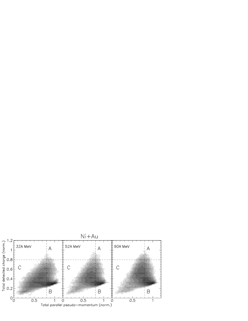
Figure 1: $Ni+Au$ INDRA data. Correlation between the total detected charge and the total parallel pseudo-momentum for $32A$ (left), $52A$ (middle) and $90A$ MeV (right). The dashed lines correspond to $80\%$ of the total detected charge and parallel pseudo-momentum.

The criterion applied for this system retains indeed too few events (less than $0.1\%$ [25]) for being reasonably considered. Obviously, we can slightly release the condition on the total detected charge to increase the number of retained events, but it turns to be somewhat arbitrary since no singularities appears in the $Z_{tot}$ distribution. Other selections have been also considered (light charged particles multiplicity or tranverse energy) but the conclusions remain unchanged.

Therefore, we have prefered to develop a new method which takes advantage of the exclusive measurements by requiring the overall information given by the experimental apparatus, without asking a priori any criterion for the detection completeness. This method is based upon the features of multidimensional analyses. Many kinds of multidimensional analyses can be employed and some of them have been already used successfully in the heavy-ion induced reactions domain [26, 27, 28]. Among them, we have chosen the Principal Component Analysis ($PCA$) for its simplicity, and because it is closely related to more conventional selection methods using global variables.

3.2 Basics

We start from a set of global variables, commonly used in heavy-ion physics such as multiplicities (light charged particles - LCP, $0<Z<3$ - and intermediate mass fragments - IMF, $Z>2$ - ), transverse energy, event shape in momentum space (eigenvalues of the kinetic flow tensor, flow angle), detection observables (total detected charge, parallel momentum, etc … ). The total number of global variables used in this study is $M=24$ and has been set in order to cover all the experimental information that can be accessed from the data after different tries. We then build the covariance matrix $V$ of these global variables which matrix elements $V_{ij}$ are defined as :

$$V_{ij}=\Sigma_{k=1}^{N}\hat{X}_{ik}\hat{X}_{jk}$$ (1)

where the indexes $i$ and $j$ run over the number of global variables ($M$) (squared $M\times M$ matrix), $k$ is the event number, $N$ is the total number of events and $\hat{X}_{ik}$ is the reduced value of the $i^{th}$ global variable for the event $k$. $\hat{X}_{ik}$ is built upon the original value $X_{ik}$ by applying the following linear transformation in order to get centred and reduced values :

$$\hat{X}_{ik}=\frac{X_{ik}-\bar{X}_{i}}{\sigma_{i}}$$ (2)

where $X_{ik}$ is the value of the $i^{th}$ global variable for event $k$, $\bar{X}_{i}$ its mean value and $\sigma_{i}$ its standard deviation over the total number of events $N$.

By diagonalizing the covariance matrix $V$, we obtain the eigenvalues and the associated eigenvectors, defining then linear combinations of these variables, called hereafter principal components [29]. These are ordered and define new planes - principal planes - where the data are projected. Since we use global variables, an event is then represented by only one point in this $M$-dimensional space.

3.3 Application to the data

The normalized eigenvalues give the statistical information carried by the associated eigenvectors and the combination of the highest eigenvalues define principal planes where the data exhaust the maximum of information [29]. Fig. 2, top row gives the spectra obtained by diagonalization of the covariance matrix for the $Ni+Au$ data at $32A$, $52A$ and $90A$ MeV. Typically, we get better than $2/3$ of the total statistical information, called explained inertia, by projecting in the first principal plane ($Pc_{max}\otimes Pc_{max-1}$), which means that we have access to a fairly large amount of information compared to simple mono- or even bi-dimensional plots.

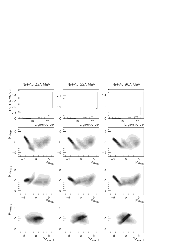
Figure 2: $Ni+Au$ INDRA data. Top row : Eigenvalues spectra extracted from the PCA for the 3 energies ($32A$, $52A$ and $90A$ MeV respectively from left to right). The dashed line represents the threshold (here $1/24$) given by assuming a random information carried by each eigenvalue. Second row : data projection in the plane defined by the two highest principal components ($Pc_{max}\otimes Pc_{max-1}$). Third row : data projection in the plane defined by the third ($PC_{max-2}$) and first ($PC_{max}$) principal components. Bottom row : projection in the plane defined by the second ($Pc_{max-1}$) and third ($Pc_{max-2}$) principal components.

Therefore, we expect to gain selectivity, compared to usual monodimensional event selection methods. Moreover, the $PCA$ gathers in a natural way events with the same features (i. e. same values of the global variables), defining thus naturally event classes as it is clearly seen on Fig. 2. The three bottom rows of Fig. 2 displays the projection obtained by combining the planes defined with the 3 highest principal components. We observe that the second row ($Pc_{max}\otimes Pc_{max-1}$) shows the best separation between the $4$ different event classes, as compared to the other planes, except for the $32A$ MeV $Ni+Au$ system (left panel). This correlates the information brought by the normalized eigenvalues and shows that the selection in the first principal plane is sufficient enough at this level to disentangle between the observed event classes.

Figure 3, top row shows again the projection of the $Ni+Au$ data on the principal plane. The inertia values, defined as the sum of the two eigenvalues, are also reported and give the amount of information carried by the projection in this plane; as already mentioned, we get around $2/3$ of the total available information. The relationship between the principal components and the global variables are given on Fig. 3 (bottom row) by the so-called correlation plot. It explains in an easy way how the data are shared out in the principal plane. For example, by looking at the total detected momentum along the beam axis ($Pz_{tot}$), we see that this quantity gets higher when we follow the direction pointed by the associated vector on the correlation plot (upper left). The corresponding direction gives then the location of the well-detected events in momentum; they corresponds to the most peripheral events (upper-left branch called $C$ on Fig. 3) and are associated with low values of the total detected charge $Z_{tot}$ since the corresponding two axes are perpendicular. Conversely, the high-multiplicity events are located almost in the opposite direction (see $M_{lcp}$ on Fig. 3) and are then practically anticorrelated with the total detected charge. The complete events (defined as the event class with the higher values of the total detected charge $Z_{tot}$) are clearly located at the rightmost part of the plot on Fig. 3 (called zone $A$). By selecting the different zones as presented on Fig. 3, we are then able to naturally separate and study the different event classes from peripheral (incomplete events) to the most dissipative collisions (pseudo-complete events).

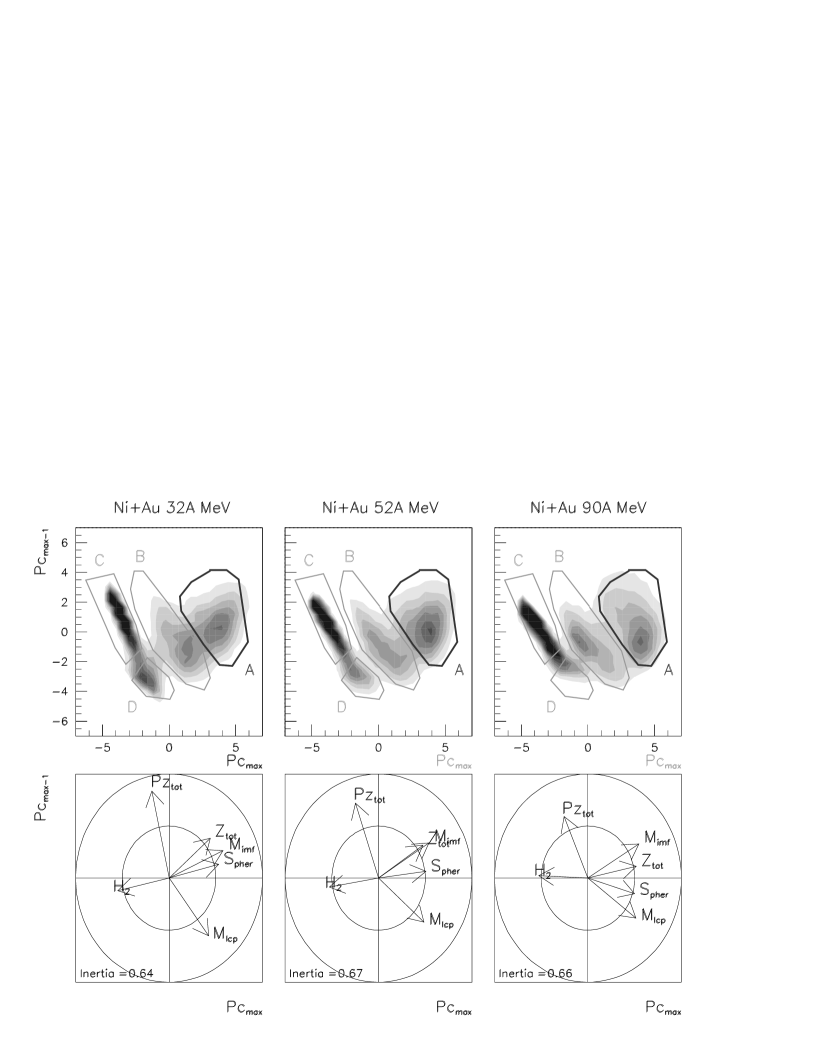
Figure 3: $Ni+Au$ INDRA data. Top row : Projection in the principal plane $Pc_{max}\otimes Pc_{max-1}$ for $32A$ (left), $52A$ (middle) and $90A$ (right) MeV. Bottom row : correlation plot for selected global variables.

We have checked that the rightmost zone, called $A$, is here associated to the highest values of the total detected charge and light charged particle multiplicity while the zones $B$, $C$ and $D$ are associated to smaller values as shown in table 1 for the $52A$ MeV $Ni+Au$ system. Table 1 gives the mean multiplicities (light charged particles and intermediate mass fragment) and the total detected charge per event. As already observed before from the correlation plot, zone $A$ corresponds to the highest values (the mean IMF multiplicity is equal to $4.0$), and groups the best-detected (total charge) and most dissipative (high multiplicity) events. In the following, we will only retain this zone because it contains the multifragmentation events (among other dissipative events) coming from a composite system formed in very central collisions.

	Zone $A$	Zone $B$	Zone $C$	Zone $D$
$<M_{LCP}>$ ($Z\leq 2$)	16.6	13.6	5.0	14.2
$<M_{IMF}>$ ($Z\geq 3$)	4.0	2.5	1.5	1.5
$<Z_{TOT}>$	48.0	34.7	28.0	27.6

Table 1: $52A$ MeV $Ni+Au$ data. Mean light charged particles multiplicity ($M_{LCP}$), IMF multiplicity ($M_{IMF}$), total detected charge ($Z_{TOT}$) for events from Zones $A$ to $D$ of Fig. 3.

Furthermore, a detailed study of the other classes [25] -not presented here- has shown that Zone $B$ is associated to incomplete fusion events where the fused system undergoes fission (mid-peripheral collisions), Zone $C$ to peripheral collisions where the quasi-projectile is close to the projectile (Nickel) and Zone $D$ to binary dissipative collisions where a (damped) quasi-projectile still survives in the exit channel.

3.4 Multifragmentation selection

The events belonging to zone $A$ of Fig. 3 (best detected and dissipative events) are kept and a second $PCA$ is applied on this sample in order to refine the selection on central events. This second $PCA$ allows a more precise ordering of the events of zone $A$ by enlarging the selectivity. In this way, we only need to work on the first principal plane ($Pc_{max}\otimes Pc_{max-1}$), and we do not need to look at the other principal planes.

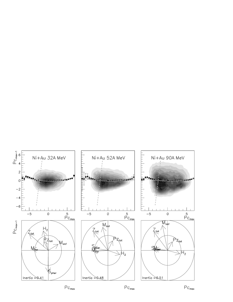
Figure 4: $Ni+Au$ INDRA data. Second $PCA$. Top row : Projection in the principal plane $Pc_{max}\otimes Pc_{max-1}$ for $32A$ (left), $52A$ (middle) and $90A$ (right) MeV. Bottom row : correlation plot for selected global variables.

The result of this second $PCA$ is displayed on Fig. 4 (top row) and the corresponding correlation plot is given in the bottom row. We see that the events are grouped together in an elongated shape along $Pc_{max}$ and there is no more any separation between event classes, showing thus that the primary selection (first $PCA$) was sufficient to get the gross features of this selected event sample. Nevertheless, we can define a ridge line from the mean values represented by the symbols (displayed as the thick curve on Fig. 4, top row ) and then cut perpendicularly as represented by the vertical dashed line on the left of the panels of Fig. 4. If we now look at the correlation plots, we see that the leftmost zone is associated to the best detected events ($Z_{tot}$), the highest LCP multiplicity $M_{lcp}$ and the most compact shape in momentum space (represented by the sphericity $S_{pher}$). At the opposite, the rightmost zone is characterized by events with an elongated shape in momentum space, as represented by the highest $H_{2}$ values [15]. It is interesting to note that the maximum IMF multiplicity ($M_{imf}$) is obtained for events on the right part of the projection plot for the $32A$ MeV $Ni+Au$ system and is associated to peripheral (elongated) and not central events. This surprising result is very well explained by the detection response of INDRA; in the $32A$ MeV case, the small value of the recoil velocity of the composite system in central collisions does not allow to overcome the energy thresholds of INDRA for the heavy products, so the IMF multiplicity does not reflect the true multiplicity for the central collisions and the experimental apparatus miss more likely the heavy and slow fragments in this case.

The ridge line displayed on Fig. 4 defines a new curvilinear abscissa called geodesic $g$ and allows a refined event sorting. Figure 5 presents the evolution of the geodesic (top row), the LCP multiplicity (middle row) and the total detected charge (bottom row) as a function of this curvilinear abscissa which is dimensionless : the origin of the curve is set at the location of the dashed line on Fig. 4, top row so that events with negative $g$ values correspond to the selection we are going to apply on the data. The number of retained events has been chosen in order to get the same amount of data for the different incident energies and to keep homogeneous values for the global variables (multiplicities, tranverse energy). It corresponds to a measured cross-section of $100mb$ ($b<1.7fm$).

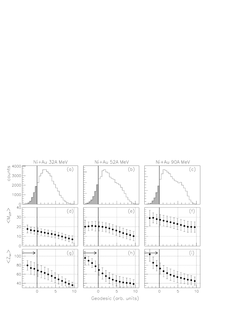
Figure 5: $Ni+Au$ INDRA data. Geodesic (top row) distribution, Mean LCP (middle) and total detected charge (bottom) as a function of the geodesic. The symbols correspond to the data. The hatched area on the geodesic distributions shows the selected events (see text).

By selecting events with negative $g$ values as presented on Fig. 5, top row by the hatched area, we get the highest LCP multiplicities and the best charge detection (around and above $80\%$ the initial total charge). The selection operated by the cut along the geodesic retains only events with the highest multiplicities, compacity and detection efficiency, providing thus multifragmentation event samples which are extensively studied in the following sections.

3.5 Generic features

Figure 6 displays the LCP and IMF multiplicities, and the atomic number vs. parallel c.m. velocity plot (along the beam direction). The multiplicities are quite large and correspond a priori to what we expect from multifragmentation event features. At $32A$ MeV, the IMF multiplicity is dominated by the 3-IMF channel while it goes to $5-6$ IMFs for $52A$ and $90A$ MeV. It is interesting to note that the IMF production saturates above $50A$ MeV (see the IMF mean values on Fig. 6). The only change between $52A$ and $90A$ MeV is then the IMF size, which decreases.

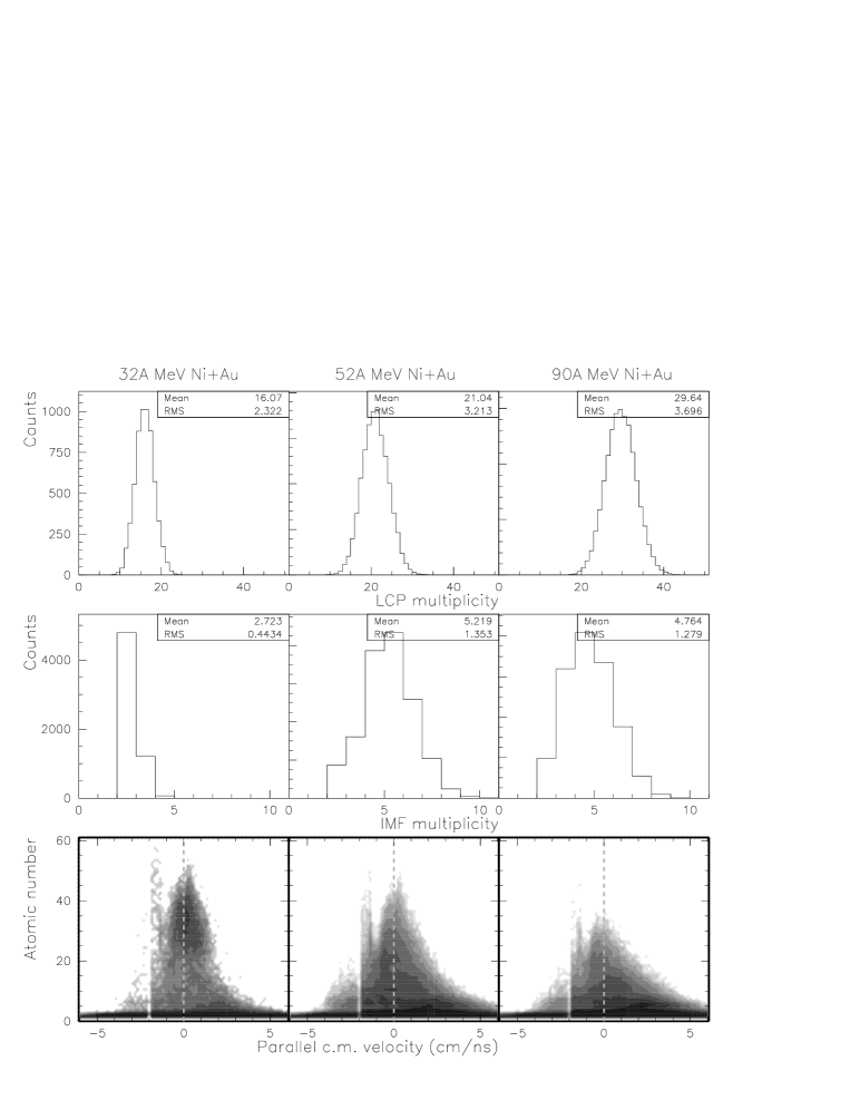
Figure 6: $Ni+Au$ multifragmentation data. Top row : LCP multiplicity. Middle row : IMF multiplicity. Bottom row : atomic number vs parallel c.m. velocity.

The correlation between the parallel c.m. velocity and the atomic number (Fig. 6, bottom row) shows a symmetric emission of the products around the center of mass of the reaction (represented by the dashed line), except for the light charged particles ($Z<5$) where a forward-peaked contribution is visible. The energy thresholds of the experimental apparatus appears at backward angles in the c.m. and truncate the velocity distribution of the backward area, showing the difficulty to get fully detected events for this asymmetrical system with INDRA (and justify the use of the multidimensional analysis). We will come back to this point in section 4.

3.6 Fragmentation pattern for central collisions

Figure 7 presents the correlation between the two heaviest fragments in the event for the $32A$ MeV(a) , $52A$ MeV(b) and $90A$ MeV(c) $Ni+Au$ system respectively. We can see clearly two zones for the first two panels (a) and (b) : an asymmetrical fragmentation pattern (a heavy fragment with Z around 35 is emitted co ncidentally with a small one, Z $\approx$ 5 ), called zone $1$ and a symmetric fragmentation pattern (the atomic number of the two heaviest fragments is around $15-20$) called zone $2$, while only the zone corresponding to the symmetric channel is present on panel (c).

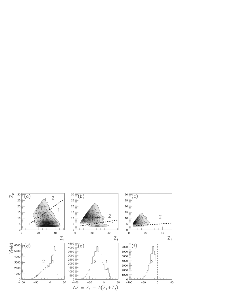
Figure 7: $Ni+Au$ data at 32 (a,d), 52 (b,e) and 90 AMeV (c,f) (central collisions). Top row : correlation between the atomic numbers of the two heaviest fragments. Bottom row : charge asymmetry $\Delta Z$ defined as $\Delta Z=Z_{1}-3(Z_{2}+Z_{3})$.

The separation between these zones depends on the incident energy because of the different IMF yields. This is shown on the bottom row of figure 7 by the ”$\Delta Z$” distribution (built with the the three largest atomic numbers $Z_{1},Z_{2}$ and $Z_{3}$) where the panel (d) and (e) exhibits a shoulder which corresponds respectively to zone 2 (at $32A$ MeV) and 1 (at $52A$ MeV). The definition of $\Delta Z=Z_{1}-3(Z_{2}+Z_{3})$ is here arbitrary and only reflects the best separation we can found between the two zones.

In order to check that the two fragmentation channels determined from Fig. 7 are not an artifact of the experimental setup (via a different detection response of INDRA), we have plotted on Fig. 8 the LCP multiplicity and the total detected charge for the $2$ zones of Fig. 7 for the $52A$ MeV $Ni+Au$ system. If we assume that the LCP multiplicity is related to the event dissipation, we can then conclude from Fig. 8a that the events belonging to both zones are associated to the same class of dissipation. Indeed, the $PCA$ selection insures us that the selected central collision samples present homogeneous properties with respect to every global variable used to build the $PCA$, as already explained in section 3. The total detected charge distributions (b) are comparable, and show that the event classes have the same detection features, despite their different fragmentation patterns. It demonstrates that experimental biases can not account for the difference in the fragmentation pattern and corresponds indeed to the coexistence of two different decay channels in the multifragmentation data.

Figure 8: $52A$ MeV $Ni+Au$ data (central collisions). LCP multiplicity (a) and total detected charge (b) for the zone $1$ (symbols) and $2$ (histogram).

In the following, we will restrain the study to the events of zone $2$ (symmetric channel), which are considered as true (simultaneous) multifragmentation events, while the other channel is likely related to a residue-evaporation/fission process and is rather ascribable to a sequential fragment production mechanism. This statement is also supported by the $\gamma$-IMF correlation analyses made for the same system at $30A$ and $45A$ MeV by the MEDEA collaboration [30] where a change from sequential to simultaneous IMF production is observed for central collisions. Anyway, the separation between these two patterns is cleaner at $52A$ MeV and $90A$ MeV (where only Zone $2$ is present), while it is difficult to define it at $32A$ MeV because of the continuity of the $\Delta Z$ distribution. Therefore we will only consider the events of Zone $2$ coming from the central collisions isolated at $52A$ and $90A$ MeV. Nevertheless, it is important to note the coexistence of these two decay channels for the central collisions of the $Ni+Au$ system at $32A$ and $52A$ MeV, which have been already reported [31] and will be discussed in the framework of phase transition in a forthcoming paper [32].

4 Multifragmentation and equilibration

4.1 Comparison protocol

In order to check the degree of equilibration of the multifragmentation events (defined as Zone $2$ in the previous section), we need to compare the experimental data to the predictions of a model based upon the statistical equilibrium hypothesis. Therefore we have used the well-known Statistical Multifragmentation Model (SMM) of Bondorf et al [33] and applied it to the $Ni+Au$ multifragmentation events.

Figure 9: Multifragmentation data. Left column : angular distribution in the c.m. for IMFs with $3<Z<8$ (open symbols) and $Z>8$ (solid symbols). The hatched area corresponds to the selection (see text). Right column : excitation energy estimated from calorimetry. The dashed area on the bottom panel is explained in section 5.2

From previous studies, it has been shown that central collisions in the Fermi energy domain can be affected by a pre-equilibrium component, even for IMFs [34]. This component is forward-peaked for the $Ni+Au$ system as illustrated on Fig. 9. The light fragments and particles are more affected by this effect. The heavy fragments have a flatter distribution along the overall angular range despite the lack of them for the most backward angles as already mentioned for Fig. 6. As a matter of fact, central collisions emit products with low velocities in the laboratory, and the determination of the recoil velocity becomes rather difficult because of the energy thresholds imposed by the experimental setup [24]. These two limitations have to be taken into account if we want to compare the data with models. Therefore, we have decided to make the comparisons in a restricted angular domain in the center of mass (c.m.). This domain is located around the transverse direction for two reasons; firstly to minimize the effect of a bad determination of the recoil velocity (because of the lack of detection for slow fragments), and secondly to exclude in a large extent the pre-equilibrium component. The angular range intervals have been set to the same values at $52A$ and $90A$ MeV and are defined as $60-120^{o}$ (hatched area on the left column of Fig. 9) in order to get reasonably flat angular distributions. In the following, all the presented data will be selected in this c.m. angular range.

Figure 9 presents also the excitation energy obtained by calorimetry [35] calculated in an event-by-event basis; the light charged particles and light IMFs (up to $Z=4$) have been taken in the restricted c.m. angular range ($60-120^{o}$) and their contribution has been multiplied by 2. The evaporated neutron contribution has been estimated from the $N/Z$ ratio of the initial system and their kinetic energy is deduced from the temperature determined by the kinetic equation of state as precised in ref. [36]. The distributions are quite broad and do not only reflect the fluctuations in the energy deposition but also the uncertainties brought by the experimental determination (neutrons, pre-equilibrium component not completely removed, detection). Nevertheless, we can note the mean values ($4.2$,$6.4$,$8.3A$ MeV for respectively $32$,$52$,$90A$ MeV) and use them as starting points for the following model comparisons.

Table 2 gives the available c.m. energy (total and per nucleon) for the studied systems and by comparing with the extracted excitation energy values we have an estimation of the percentage of deposited energy as a function of the asymmetry of the system (when comparing $Ni+Au$ to $Xe+Sn$) or the incident energy ($Ni+Au$). The value for the $Xe+Sn$ system ($9.3A$ MeV) has been obtained by using the same prescription [25].

System	$E_{inc}$ ($A$MeV)	$E_{cm}$ (MeV)	$E_{cm}$ (MeV/n)	$E^{*}/E_{cm}$
${}^{58}Ni+^{197}Au$	32	1430	5.6	0.81
${}^{58}Ni+^{197}Au$	52	2320	9.1	0.70
${}^{58}Ni+^{197}Au$	90	4000	15.7	0.53
${}^{119}Xe+^{nat}Sn$	50	3080	12.4	0.73

Table 2: Incident energy $E_{inc}$, available c.m. energy $E_{cm}$ and ratio of estimated deposited energy $E^{*}/E_{cm}$ for the studied systems.

The ratio between the deposited energy (estimated by calorimetry) and the c.m. available energy decreases as a function of the incident energy from $0.8$ at $32A$ MeV to $0.5$ at $90A$ MeV for the $Ni+Au$ system; it shows the ever increasing part of the preequilibrium component when going from Fermi energy toward the relativistic regime. Moreover, we do not observe any dependence of the ratio ($\approx 0.7$) as a function of the mass asymmetry of the entrance channel for a given incident energy (here $50A$ MeV). Thus, no transparency effects are evidenced at that incident energy.

4.2 Partitions

Figure 10 presents the results obtained for the comparison between the experimental data (here $52A$ MeV $Ni+Au$) and the simulation (SMM) for the best set of input parameters we have found; it corresponds to a source size of $A=215$ ($Z=86$) with an thermal excitation energy of $E^{\ast}/A=6.5MeV$. This latter value is close to the one obtained experimentally by calorimetry ($<E^{\ast}/A>=6.4$ MeV) [25] and fig. [article9] right. Several attempts have been made in order to determine the optimal freeze-out volume in the model but due to the comparison in a rather small angular range, no sensitivity to this parameter has been found and we have taken the usual value of $3V_{0}$ for the freeze-out configuration.

The data (symbols) for the $52A$MeV $Ni+Au$ system are fairly reproduced by the model (histogram) as far as partitions are concerned. The atomic number distribution (Fig. 10a) exhibits some discrepancies for charges between $20$ and $35$ but the global trend of the distribution is reproduced. It has to be mentioned that the spectra of Fig. 10a are normalized to the number of events. The LCP multiplicity (Fig. 10b) and the fragment multiplicity ($Z>5$, Fig. 10c) are slightly overestimated by the model while the charge of the heaviest fragment (Fig. 10d) gets the same agreement as the inclusive charge distribution. The events generated by SMM have been passed through a software replica of the INDRA array and the comparisons are made into a restricted angular range domain in the center of mass (here between $60$ and $120$ degrees) in order to minimize the threshold biases and pre-equilibrium effects [25, 35], as already explained in section 4.1.

Figure 10: Atomic number (a) for the $52A$ MeV $Ni+Au$ data (symbols) and SMM (histogram), LCP multiplicity ($Z\leq 2$) (b), Fragment multiplicity ($Z\geq 6$) (c) and atomic number distributions of the heaviest fragment (d). These comparisons are made in a restricted angular domain in the center of mass ($60-120^{o}$). All spectra are normalized to the number of events.

Some attempts have been made in order to get a more quantitative comparison between the data and the model predictions, such as it is preconized in [37] by the backtracing method. The results show that the confidence intervals where the data are reasonably reproduced are $0.5A$ MeV for the excitation energy and $5$ charge units for the source size. This agreement has been numerically evaluated by the calculation of a $\chi^{2}$ upon the $4$ distributions presented on Fig. 10. The confidence intervals given here refer to minimal $\chi^{2}$ values which do not differ from more than $10\%$, and the values reported for the model corresponds to the central points of these intervals.

Figure 11: Atomic number distribution (a) for the $90A$ MeV $Ni+Au$ data (symbols) and SMM (histogram), LCP multiplicity ($Z\leq 2$) (b), Fragment multiplicity ($Z\geq 6$) (c) and atomic number distributions of the heaviest fragment (d). These comparisons are made in a restricted angular domain in the c.m. ($60-120^{o}$). All spectra are normalized to the number of events.

The same comparison has been made for the $90A$MeV $Ni+Au$ system and is presented on Fig. 11. The input parameters of SMM are now $A=215$ ($Z=86\pm 5$) and $E^{*}/A=7.5\pm 0.5$ MeV. The agreement is satisfactory between the model and the data, showing then that the fragment partitions are also consistent with a statistical exploration of the available phase space as it is suggested in the SMM model.

4.3 Kinetic properties

Figure 12 shows the correlation between the mean kinetic energy (in the c.m.) and the atomic number for the data (solid circles) and the model (open symbols). An agreement is accounted for the heaviest atomic number ($Z>15$) as displayed on Fig. 12 (left panel for $52A$MeV and right for $90A$MeV). However, the model underestimates in a large extent the mean kinetic energies for light charged particles and IMFs ($Z<10$). If we assume an extra collective energy (radial flow) of $0.5A$MeV in the model (open triangles) , then the mean kinetic energies are slightly better reproduced for $Z<10$ but the agreement fails totally for the heavier products.

Figure 12: Mean c.m. kinetic energy versus atomic number for the multifragmentation events of the $Ni+Au$ system at $52A$ MeV (left) and $90A$ MeV (right) (solid circles), SMM calculations without radial flow (open circles) and SMM calculations with $0.5A$ MeV of radial flow (triangles).

We can therefore conclude that no radial flow has to be put in SMM calculations to reproduce the kinetic properties of fragments while strong out-of-equilibrium features appear for light charged particles and light IMFs ($Z<10$). This result is somehow consistent with the conclusions made from the $Ar+Au$ analysis in the same incident energy range [38] where is evidenced an expansion energy component; indeed, in this case, only kinetic energy distribution for light IMFs ($Z<10$) have been analysed and give the same mean values as our analysis. This important point will be furthermore developed in the next section by the direct comparison between experimental data.

5 Experimental comparisons

At this point, we have shown that the multifragmentation events are compatible with a scenario of statistical partitions as predicted by SMM. We will now go further by systematically comparing data coming from systems with different entrance channels. To do so, we will use the same ${}^{58}Ni+^{197}Au$ multifragmentation events as before (at $52A$ and $90A$ MeV) but also a new one obtained by the same selection method ($PCA$) onto the $50A$ MeV ${}^{129}Xe+^{nat}Sn$ system [25, 35]. We will have then 2 systems with different mass asymmetries in the entrance channel ($Xe+Sn$, $Ni+Au$), and two incident velocities ($50A/52A$, $90A$MeV) and will present in the following the cross-comparisons between them.

5.1 Same incident energy

Figure 13: Comparison between $52A$ MeV $Ni+Au$ and $50A$ MeV $Xe+Sn$ multifragmentation data. Atomic number (a), LCP multiplicity (b) , IMF multiplicity (c) and correlation between the mean c.m. kinetic energy and the atomic number (d) ($Ni+Au$ : circles, $Xe+Sn$ : triangles). These comparisons are made in a restricted angular domain in the c.m. ($60^{o}-120^{o}$). All spectra are normalized to the number of events. The LCP and IMF multiplicities have been multiplied by two in order to reflect the integrated values.

The comparison between two systems ($52A$ MeV $Ni+Au$ and $50A$ MeV $Xe+Sn$) of nearly the same incident velocity and the same total size ($250$ nucleons) is presented on Fig. 13. The data correspond to multifragmentation samples (using the $PCA$ selection), and have been characterized by almost the same source size ($<Z>=85$ for the $50A$ MeV $Xe+Sn$ system) but different thermal excitation energies ($7.5A$ MeV compared to $6.4A$ MeV for $Ni+Au$ once substracted the radial energy component) [25, 35]. We see clearly that the charge distribution (13a) or the LCP (13b) multiplicities (multiplied by 2 in order to get integrated values) extend higher for the $50A$MeV $Xe+Sn$ system as expected by the thermal excitation energy difference of about $1A$ MeV. Conversely, the IMF multiplicities (13b) are similar but only reflect the counterbalance between the higher IMF ($3<Z<15$) and the smaller heavy fragment ($Z>15$) yields for the $Xe+Sn$ system.

Figure 13d shows the mean c.m. kinetic energies as a function of the atomic number. We see here that the light charged particles (up to Lithium) are superimposed (insert of Fig.13 d) while a major discrepancy appears for heavier fragments. Indeed, in the $Xe+Sn$ system case, a radial energy component has to be invoked as shown in [15, 35]. This is not the case for the $Ni+Au$ system for which one does not observe the linear increase of the mean kinetic energy as a function of the fragment charge, as expected if there is a radial flow component.

5.2 Same thermal excitation energy

The comparison is now made between the $50A$ MeV $Xe+Sn$ and $90A$ MeV $Ni+Au$ systems (Fig. 14). Here, the mean thermal excitation energy components, determined experimentally and by comparison with the SMM model, are nearly equivalent [25] and are around $7.5-8A$ MeV. Nevertheless, we decide to present the data with a condition on the (thermal) excitation energy because of the broadness of the excitation energy distribution (more than $7A$ MeV for the $Ni+Au$ system); to do so, we have gated around the most probable excitation energy value (see the dashed area on Fig. 9, bottom panel of the right column), and it corresponds here to $7.7\pm 1.5A$ MeV. In this way, the excitation energy domain is similar for both systems.

Figure 14: Comparison between $90A$ MeV $Ni+Au$ and $50A$ MeV $Xe+Sn$ multifragmentation data. Atomic number distribution (a), LCP multiplicity (b), IMF multiplicity (c) and correlation between the mean c.m. kinetic energy and the atomic number (d) ($Ni+Au$ : open circles, $Xe+Sn$ : solid triangles). These comparisons are made in a restricted angular domain in the c.m. ($60^{o}-120^{o}$). The data have been gated around the following excitation energy interval : $6-9A$ MeV. All spectra are normalized to the number of events. The LCP and IMF multiplicities have been multiplied by two in order to reflect the integrated values.

From Figure 14a, we see that the atomic number distributions are nearly identical, and that the LCP and IMF multiplicities (14b and 14c) are comparable, showing that the fragmentation pattern is equivalent between these two systems, and is governed by the thermal excitation energy stored into the system. This result means that the partitions are similar whatever the radial flow is. Figure 14d, displaying the mean c.m. kinetic energy as a function of the charge shows a disagreement for fragments ($Z>3$), while the situation is different for light charged particles ($Z<4$) as seen in the insert. For these particles, the mean kinetic energies are higher for the $Ni+Au$ system, as expected for pre-equilibrium emission, mainly sensitive to the incident energy. The large disagreement observed for fragments is attributed to the existence of an additionnal collective energy in the $Xe+Sn$ system of $2A$MeV [28, 35]. Putting together these obsevations, it demonstrates the decoupling between the thermal and the radial flow components of the excitation energy. This statement seems to be valid in the limit of a small ratio between the collective and the thermal component because large deviations to the decoupling have been found at higher incident energies [39, 40].

5.3 Excitation function of the $Ni+Au$ system

At last, comparisons for the same system ($Ni+Au$) at different incident energies ($52A$ and $90A$ MeV) are presented in Fig. 15. The fragmentation pattern is different as illustrated on Fig. 15 (atomic number (a) and LCP multiplicity (b) distributions). Figure 15c presents the IMF multiplicities which are surprisingly equivalent. It means that the maximum number of fragments has been already reached for the central collisions of the $Ni+Au$ system between $52A$ and $90A$ MeV, while the LCP multiplicity continues to increase (Fig. 15b); in fact, this is the size of the fragments which decreases when going from $52A$ to $90A$ MeV but not their yield. Systematic studies of IMF production for symmetric systems [41, 42, 43] have shown that a maximum was reached at incident energies increasing with the mass of the system and was located around $100A$ MeV, while it has been found at smaller incident energies - around $50A$ MeV - for the $Xe+Sn$ systems measured by the INDRA collaboration [44]. For the (asymmetrical) $Ni+Au$ system, we also come to the same conclusions (maximum around $50A$ MeV) and it can therefore be related to a common behavior of fused systems [24].

Figure 15: Comparison between $52A$ MeV and $90A$ MeV $Ni+Au$ multifragmentation data. Atomic number (a), LCP multiplicity (b), IMF multiplicity (c) and correlation between the mean c.m. kinetic energy and the atomic number (d) ($52A$ MeV : solid circles, $90A$ MeV : open circles). These comparisons are made in a restricted angular domain in the c.m. ($60^{o}-120^{o}$. All spectra are normalized to the number of events. The LCP and IMF multiplicities have been multiplied by two in order to reflect the integrated values.

The kinetic properties, displayed by Fig. 15d, are also similar, and substantiate the inexistence of any radial flow energy in the data. The light charged particles, shown in the insert, are systematically higher for the $90A$ MeV system (open circles) as expected both from pre-equilibrium and thermal effects.

At this point, we must recall that the source sizes, determined both from SMM comparisons and experimentally, are comparable [25]; the difference in the thermal component of the excitation energy between the two systems is roughly compensated by the difference between the Coulomb energies at the freeze-out stage, leading to the same kinetic energy profiles. This suggests that we need to compare both static and kinetic observables to get relevant information about the characteristics of fused systems formed in central collisions.

6 Conclusions

We have presented a new technique in order to carefully isolate the most violent collisions by using a multidimensional analysis named the Principal component Analysis ($PCA$). We have shown that this method can be applied for all studied systems over a large domain of incident energy (i.e. between $32A$ and $90A$MeV) and is perfectly suited for $4\pi$ devices. This provides a powerful tool to select event classes in the domain of heavy-ion induced reactions. The method have then been used to select multifragmentation data among the most dissipative collisions. The selected samples have been found to be highly dissipative and to present two different fragmentation patterns (at $32A$ and $52A$ MeV) which coexists at the same excitation energy. The first one is associated to residue-evaporation or fission-evaporation mechanism and is characterized by a big residue ($Z\approx 35$) while the second mechanism is associated to a more copious IMF production and can be related to the multifragmentation of a single source.

We have analysed the multifragmentation events from the $Ni+Au$ system at $52A$ and $90A$MeV. From the comparisons with the SMM model and between experimental data, we have evidenced that fragment partitions are mainly governed by the thermal part of the excitation energy. Conversely, for light charged particles and light IMFs, we have seen that their kinetic properties are closely related to the incident energy and mass asymmetry, enlightening thus the different emission time scales between these products and the heavier ones, showing then that only a full treatment of the dynamics of the collision can provide relevant comparison with data. No evidence for a sizeable radial flow energy has been found for the $Ni+Au$ system between $52A$ and $90A$MeV nor any dependence as a function of the incident energy. The fragmentation pattern are very similar for the $90A$ MeV $Ni+Au$ and the $50A$ MeV $Xe+Sn$ systems while the kinetic features are found to be completely different. This fact shows clearly that a decoupling between the thermal and the radial flow part of the excitation energy is achieved in this incident energy domain where the radial component is quite small as compared to the thermal one.

By comparing the observed difference in the energy deposition (thermal + expansion), we find that it is maximal for the symmetric system (conversely the pre-equilibrium component is minimised) and constitutes then the most efficient way to dissipate energy into nuclear systems. As a final conclusion, we would say that nuclei cannot be produced with thermal excitation energies greater than the value given by the average binding energy ($\approx 8A$ MeV). This means that the extra energy dissipated into the system ($50A$ MeV $Xe+Sn$ case) is then entirely converted into collective degrees of freedom such as the radial flow of particles.

References

- [1] G. Bertsch and P.J. Siemens, Phys. Lett. B126 (1983) 9
- [2] H. Schulz et al., Phys. Lett. B147 (1984) 17
- [3] P. Bonche, Ecole Joliot-Curie, Maubuisson, France (1985) 1
- [4] D. Durand, E. Suraud and B. Tamain, Nuclear dynamics in the nucleonic regime, Series in fundamental and applied Nuclear Physics, Inst. of Physics (2000)
- [5] D.H.E. Gross, Rep. Prog. Phys. 53 (1990) 605
- [6] J. Pouthas et al., Nucl.Inst. and Meth. A357 (1995) 418
- [7] G. Tabacaru et al., Nucl. Inst. and Meth. A428 (1999) 379
- [8] M. Parlog et al., Nucl. Inst. and Meth. A (in press).
- [9] J. C. Steckmeyer et al., Nucl. Inst. and Meth. A361(1996) 472
- [10] J. Cugnon and D. L’Hôte, Nucl. Phys. A397 (1983) 519
- [11] R. Bougault et al., Nucl. Phys. A488 (1998) 255c
- [12] L. Phair et al., Nucl. Phys. A548 (1992) 489
- [13] M. Louvel et al., Nucl. Phys. A559 (1993) 137
- [14] O. Lopez et al., Phys. Lett. B315 (1993) 34
- [15] N. Marie et al., Phys. Lett. B391 (1997) 15
- [16] S. Salou, PHD thesis, University of Caen (1997)
- [17] J. Lukasik et al., Phys. Rev., C55 (1996) 1906
- [18] T.M. Hamilton et al., Phys. Rev., C53 (1996) 2273
- [19] M.T. Magda et al., Phys. Rev., C53 (1996) 1473
- [20] M. d’Agostino et al., Zeit. Phys., A353 (1995) 191
- [21] T. Gharib et al., Phys. Lett. B444 (1998) 231
- [22] P. Kreutz et al., Nucl. Phys. A556 (1993) 672
- [23] A. Sch ttauf et al., Nucl. Phys. A607 (1996) 457
- [24] J.D. Frankland et al., Nucl. Phys. A689 (2001) 905
- [25] N. Bellaize, PHD thesis, University of Caen (2000)
- [26] P. Désesquelles et al., Phys. Rev. C62 (2000) 024614
- [27] A.M. Maskay, PHD thesis, University of Lyon (1999)
- [28] B. Bouriquet et al., PHD thesis, University of Caen (2001).
- [29] E. Lloyd, Handbook of Applicable Mathematics, Volume VI (Statistics), Part B, J. Wiley New York (1984)
- [30] C. Agodi et al., Proceeding of the International Workshop on Multifragmentation (IWM2001), Catania (2001)
- [31] O. Lopez et al., Contribution to the XXXIX winter meeting on Nucl. Phys., Bormio (Italy), Ed. I. Iori (2001) 61
- [32] O. Lopez et al., in preparation
- [33] J.P. Bondorf, A.S. Botvina, A.S. Iljinov, I.N. Mishustin and K. Sneppen, Phys. Rep. 257 (1995) 133
- [34] E. Colin et al., Phys. Rev., C57 (1998) 1032
- [35] N. Le Neindre, PHD thesis, University of Caen (1999)
- [36] M. D’Agostino et al., Nucl. Phys. A 650 (1999) 329
- [37] P. Désesquelles et al., Nucl. Phys. A633 (1998) 547.
- [38] R. T.de Souza et al., Phys. Lett. B300 (1993) 29
- [39] W. C. Hsi et al., Phys. Rev. Lett. 73 (1994) 3367-3370
- [40] J. Lauret et al., Phys. Rev. C57 (1998) R1051
- [41] G.F. Peaslee et al., Phys. Rev. C49, (1994) R2271
- [42] W. Reisdorf et al., Nucl. Phys. A612 (1997) 493
- [43] D. Sisan et al., Phys. Rev. C63 (2001) 027602
- [44] M. F. Rivet, Proc. int. Conf. on clustering aspects of nuclear structure and dynamics, Rab, Croatia, June 1999, ed. World Scientific, p. 278