Neutron polarizabilities investigated by quasi-free Compton scattering from the deuteron

Abstract

Measuring Compton scattered photons and recoil neutrons in coincidence, quasi-free Compton scattering by the neutron has been investigated at MAMI (Mainz) at $\theta^{\rm lab}_{\gamma}=136^{\circ}$ in an energy range from 200 to 400 MeV. From the data a polarizability difference of $\alpha_{n}-\beta_{n}=9.8\pm 3.6({\rm stat}){}^{+2.1}_{-1.1}{}({\rm syst})\pm 2.2({\rm model})$ in units of $10^{-4}{\rm fm}^{3}$ has been determined. In combination with the polarizability sum $\alpha_{n}+\beta_{n}=15.2\pm 0.5$ deduced from photo absorption data, the first precise results for the neutron electric and magnetic polarizabilities, $\alpha_{n}=12.5\pm 1.8({\rm stat}){}^{+1.1}_{-0.6}{}({\rm syst})\pm 1.1({\rm model})$ and $\beta_{n}=2.7\mp 1.8({\rm stat}){}^{+0.6}_{-1.1}{}({\rm syst})\mp 1.1({\rm model})$, are obtained.

The electromagnetic polarizabilities belong to the fundamental structure constants of the nucleon. Although attempts to measure the electromagnetic polarizabilities of the neutron have a long history the results obtained up to now have remained unsatisfactory. Since Compton scattering experiments appeared too difficult, the first generation of investigations concentrated on the method of electromagnetic scattering of low-energy neutrons in the electric fields of heavy nuclei, as measured in neutron transmission experiments. The history of these studies is summarized in Ref. [1]. The latest in a series of experiments have been carried out at Oak Ridge [2] and Munich [3] leading to $\alpha_{n}=12.6\pm 1.5\pm 2.0$ and $\alpha_{n}=0.6\pm 5$, respectively, for the electric polarizability of the neutron in units of $10^{-4}$fm³ which will be used throughout in the following. The numbers given here have been corrected by adding the Schwinger term [4] $e^{2}\kappa^{2}_{\rm n}/4M^{3}=0.6$, containing the neutron anomalous magnetic moment $\kappa_{n}$ and the neutron mass $M$, which had been omitted in the original evaluation of these experiments. After including the Schwinger term the numbers are directly comparable with the ones defined through the Compton scattering process [4]. While the Munich result [3] has a large error, the Oak Ridge result [2] is of very high precision. However, this high precision has been questioned by a number of researchers active in the field of neutron scattering [5]. Their conclusion is that the Oak Ridge result [2] possibly might be quoted as $7\leq\alpha_{n}\leq 19$. Note that the neutron transmission experiments do not constrain the magnetic polarizability $\beta_{n}$.

The method of Compton scattering makes use of the equation

$$f=f_{B}+\omega\omega^{\prime}\alpha\,{\boldsymbol{\epsilon}}\cdot{\boldsymbol{\epsilon}^{\prime}}+\omega\omega^{\prime}\beta\,{\bf s}\cdot{\bf s^{\prime}}+{\cal O}(\omega^{3}),$$ (1)

where $f_{B}$ is the Born amplitude, $\alpha$ the electric and $\beta$ the magnetic polarizability, $\omega$, $\omega^{\prime}$ the photon energies in the initial and final state, respectively, and ${\boldsymbol{\epsilon}}$, ${\boldsymbol{\epsilon}}^{\prime}$ and ${\bf s}$, ${\bf s}^{\prime}$ the directions of the corresponding electric and magnetic fields. A pioneering experiment on Compton scattering by the neutron had been carried out by the Göttingen and Mainz groups at the electron beam of MAMI A operated at 130 MeV [6]. This experiment followed a proposal of Refs.[7] to exploit the reaction $\gamma d\to\gamma np$ in the quasi-free kinematics, though there is an evident reason why such an experiment is difficult at energies below pion threshold. For the proton the largest portion of the polarizability-dependent cross section in this energy region stems from the interference term between the Born amplitude containing Thomson scattering as the largest contribution, and the non-Born amplitude containing the polarizabilities. For the neutron the Thomson amplitude vanishes so that the interference term is very small and correspondingly cannot be used for the determination of the neutron polarizabilities. This implies that the cross section is rather small being about 2–3 nb/sr at 100 MeV. The way chosen to overcome this problem was to use a high flux of bremsstrahlung without tagging[6, 7]. The result obtained in the experiment [6] was

$$\alpha_{n}=10.7^{+3.3}_{-10.7}.$$ (2)

This means that the experiment was successful in providing a value for the electric polarizability and its upper limit but it did not permit to determine a definite lower limit. The reason for this deficiency is that below pion threshold the neutron Compton cross section is practically independent of $\alpha_{n}$ if $0\lesssim\alpha_{n}\lesssim 10$ (see Refs. [7, 8]). In order to overcome this difficulty it was proposed to measure the neutron polarizabilities at energies above pion threshold with the energy range from 200 to 300 MeV being the most promising, since there the cross sections are very sensitive to $\alpha_{n}$ [7, 8] if, in addition, large scattering angles are chosen.

A first experiment on quasi-free Compton scattering by the proton bound in the deuteron for energies above pion threshold was carried out at MAMI (Mainz) [9]. This experiment served as a successful test of the method of quasi-free Compton scattering for determining $\alpha-\beta$. Later on this method was applied to the proton and the neutron bound in the deuteron at SAL (Saskatoon) [10]. In this experiment differential cross sections for quasi-free Compton scattering by the proton and by the neutron were obtained at a scattering angle of $\theta^{\rm lab}_{\gamma}=135^{\circ}$ for incident photon energies of $236-260$ MeV, which were combined to give one data point of reasonable precision for each nucleon. From the ratio of these two differential cross sections a most probable value of $\alpha_{n}-\beta_{n}=12$ was obtained with a lower limit of $0$ and no definite upper limit. Combining their results [10] with that of Eq. (2) [6] the authors obtained the following 1-sigma constraints for the electromagnetic polarizabilities $7.6\leq\alpha_{n}\leq 14.0$ and $1.2\leq\beta_{n}\leq 7.6$.

It should be noted that coherent elastic (Compton) scattering by the deuteron provides a further method for determining the electromagnetic polarizabilities of the neutron. An evaluation of first experiments [11, 12] using the theoretical model of [13, 14] gave the values of $\alpha_{n}+\beta_{n}=20\pm 3$ and $\alpha_{n}-\beta_{n}=-2\pm 3$. Progress in the application of this method may be expected from an experiment carried out at MAX-Lab [15] and from further improvements of the theoretical basis for the data analysis. Ref. [14] also provides access to further theoretical work on Compton scattering by the nucleon.

In this Letter we report on first measurements of differential cross sections for quasi-free Compton scattering by the proton and the neutron covering a large energy interval from $E_{\gamma}=200$ to $400$ MeV. This large coverage is indispensable for determining data for the electromagnetic polarizabilities with good precision. The apparatus used is shown in Fig. 1. Tagged photons produced by the tagging facility at MAMI (Mainz) entered a scattering chamber, containing a $4.6{\rm cm}\,\O\!\times 16.3{\rm cm}$ lq.  hydrogen or lq.  deuterium target in a Kapton target cell. The $48{\rm cm}\,\O\!\times 64{\rm cm}$ NaI(Tl) detector was positioned at a distance of 60 cm from the target center at a scattering angle of $\theta^{\rm lab}_{\gamma}=136^{\circ}$ as the largest angle convenient for an experimental set-up. A scintillation counter in front of the collimator is used to identify and veto charged particles. As a recoil detector the Göttingen SENECA detector was used, positioned at a distance of 250 cm. SENECA was built as a neutron detector capable of pulse-shape discrimination. It is a honeycomb structure of 30 hexagon-shaped detector cells of 15.0 cm minimum diameter and 20.0 cm length filled with NE213 liquid scintillator. The entrance face is covered by four plastic scintillators to discriminate between charged and neutral particles. In the present experiment SENECA served as the stop detector of a time-of-flight measurement, with the start signal provided by the $48{\rm cm}\O\!\times 64{\rm cm}$ NaI(Tl) detector.

Data were collected during 238 h of beam time with a deuterium target and about 35 h with a hydrogen target. The tagging efficiency was about $55\%$, measured several times during the runs by means of a Pb-glass detector in the direct photon beam, and otherwise monitored by a P2 type ionization chamber positioned at the end of the photon beam line. The neutron detection efficiency $\epsilon_{n}$ was experimentally determined in situ via the reaction $p(\gamma,\pi^{+}n)$. The charged pion was identified by the veto counter in front of the NaI(Tl) detector and through the missing $\pi^{+}$-energy

$${\rm E}_{\pi^{+}}^{{\rm miss}}={\rm E}_{\pi^{+}}^{{\rm calc}}-{\rm E}_{\pi^{+}}^{{\rm NaI}},$$ (3)

where ${\rm E}_{\pi^{+}}^{{\rm calc}}$ is the energy of the $\pi^{+}$ meson calculated from the incident photon energy and from the $\pi^{+}$ emission angle, and ${\rm E}_{\pi^{+}}^{{\rm NaI}}$ the $\pi^{+}$ energy measured by the NaI(Tl) detector. The result obtained for the neutron detection efficiency is $\epsilon_{n}=0.180\pm 0.014$ and proved to be in good agreement with previous measurements [16].

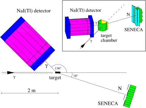
FIG. 1.: Experimental arrangement used for the present experiment on Compton scattering by the proton and quasi-free Compton scattering by the proton and the neutron. Compton scattering events were identified through coincidences between the Mainz 48 cm $\O$ $\times$ 64 cm NaI(Tl) photon detector positioned at $\theta^{\rm lab}_{\gamma}=136^{\circ}$ and the Göttingen segmented recoil counter SENECA positioned at $\theta^{\rm lab}_{N}=18^{\circ}$. The inset shows a perspective view of this arrangement.

Figure 2 shows typical spectra of photon events measured in coincidence with a recoil nucleon obtained from a deuteron target. In the left panels the recoil nucleon was identified to be a proton, in the right panels a neutron. For the data analysis a two dimensional procedure was applied with the missing nucleon energy ${\rm E}^{\rm miss}_{N}={\rm E}^{\rm calc}_{N}-{\rm E}^{\rm\,SEN}_{N}$ and missing photon energy ${\rm E}^{\rm miss}_{\gamma}={\rm E}^{\rm calc}_{\gamma}-{\rm E}^{\rm NaI}_{\gamma}$ as the parameters, where ${\rm E}^{\rm\,SEN}_{N}$ and ${\rm E}^{\rm NaI}_{\gamma}$ denote measured energies and ${\rm E}^{\rm calc}_{N}$ and ${\rm E}^{\rm calc}_{\gamma}$ the corresponding energies calculated assuming a Compton event. In this way optimal use of the separation of the two types of events as provided by the resolution of the apparatus has been made. For the spectra shown this separation of the two types of events was optimized by appropriately rotating the scatter plot of events around the origin of the ${\rm E}^{\rm miss}_{N}-{\rm E}^{\rm miss}_{\gamma}$ plane before the projection of the data on the new abscissa – ${\rm E}^{\rm miss}_{\rm rot}$ – was carried out. The experiment was accompanied by a complete Monte Carlo simulation. The curves shown in Fig. 2 are the results of this Monte Carlo simulation after adjusting them to the Compton events (grey areas) and to the $\pi^{0}$ events (white areas), respectively. It is apparent, that at the lowest photon energies of $\sim$ 230 MeV there is a complete separation of the two types of events. This separation remains possible up to about 380 MeV.

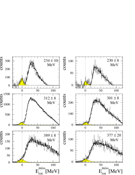
FIG. 2.: Spectra of photon events registered in coincidence with a recoil nucleon versus the missing energy of the photon E${}^{\rm miss}_{\rm rot}$ defined in the text. Left panels: recoil protons identified. Right panels: recoil neutrons identified. The curves are the results of a complete Monte Carlo simulation adjusted to the Compton scattering events (grey areas) or to the $\pi^{0}$ events (white areas).

For the free proton differential cross sections may be calculated from the number of measured Compton events using a complete Monte Carlo simulation of the experiment to determine the detection efficiency. For the quasi-free reaction the same procedure may be applied. However, in this case an effective differential cross section is obtained in this first step of data analysis which requires a second step to take into account the effects of binding of the nucleon in the deuteron. These effects of binding manifest themselves in the Fermi momentum distribution of the nucleons. In addition, effects due to final state interaction of the emitted particles and due to meson exchange currents have to be taken into account. A detailed description of these processes has been given in Ref. [7]. The result of the second step of the data analysis is the triple differential cross section in the center of the quasi-free peak of the recoil nucleon determined from the effective differential cross section as obtained from the number of measured Compton events. For this determination an appropriate Monte Carlo simulation has to be taken into account.

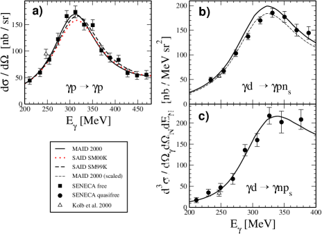
FIG. 3.: Differential cross sections for Compton scattering at $\theta^{\rm\,lab}_{\gamma}$ = 136^∘: (a) Hydrogen target with the recoil proton detected in coincidence, (b) deuterium target with the recoil proton detected in coincidence and the neutron serving a spectator (s), (c) deuterium target with the recoil neutron detected in coincidence. Predictions: (a) Nonsubtracted dispersion theory [17] using the MAID2000 (solid line), SAID-SM00K (dotted) and SAID-SM99K (dashed) parametrizations. (b) Solid line: Same as the solid line in (a) but calculated for the quasi-free reaction on the proton [7]. Dashed line: Same as the solid line but multiplied with a scaling factor of 0.93. (c) Same as the solid line in (b) but for the neutron. The curve is calculated for $\alpha_{n}-\beta_{n}=9.8$. The SAL results [10] are shown by triangles.

Figures 3a-c show the results of the present experiment. The experimental data for the free proton shown in Fig. 3a are compared with predictions based on the nonsubtracted dispersion theory as described in Ref. [17] and thoroughly tested in Refs. [18, 19]. In these former experiments it was shown that the parametrizations SAID-SM99K [20] and MAID2000 [21] led to a good agreement with the experimental differential cross sections for Compton scattering by the proton in the $\Delta$ resonance region, whereas the more recent parametrization SAID-SM00K led to too small differential cross sections. Exactly the same observation is made in the present work. Therefore, the parametrization SAID-SM00K was disregarded in the further data analysis. Going a step further, Fig. 3a may be used to find arguments in favor of either the MAID2000 or the SAID-SM99K parametrization. Though the differences are small, there is a slight preference for the MAID2000 pameterization which is seen in Fig. 3a and reflected by the $\chi^{2}$ values. Therefore, we decided to base the further evaluation on the MAID2000 parametrization and to use the SAID-SM99K parametrization only for getting an estimate for the model error connected with imperfections of the photomeson amplitudes.

In Fig. 3b a test of the method of quasi-free Compton scattering is carried out. The data shown are triple differential cross sections for quasi-free Compton scattering by the proton in the center of the quasi-free peak with their statistical errors. The systematic errors amount to $\pm 4.4\%$. The solid curve in this figure shows triple differential cross sections for quasi-free Compton scattering by the proton in the center of the quasi-free peak. This theoretical prediction has been obtained in the model of Ref. [7] on the basis of the MAID2000 parametrization. The $NN$-interaction entering into this model has been taken from the CD-Bonn potential [22]. For comparison also the separable representation of the Paris potential [23] has been applied, leading to essentially no difference. The overall agreement between experiment and prediction as given by the solid curve may be considered as satisfactory, although there is some deviation visible in the energy range between 270 and 300 MeV. At present we do not have an explanation for this residual deviation which, therefore, could not be eliminated by means of a correction. Consequently, we have to treat it as a possible source of uncertainty which has to be taken into account through a further contribution to the model error. In order to get a quantitative result for this additional model error, the prediction shown in Fig. 3b as a solid curve has been scaled down by a factor of 0.93 to give the dashed curve. Through this procedure we arrive at a modified set of photomeson amplitudes which may be used in the further analysis to estimate the additional model error connected with a possible imperfection of the theory of the quasi-free Compton scattering.

Figure 3c shows triple differential cross sections for the neutron in the center of the quasi-free peak compared with predictions obtained in the model of Ref. [7] on the basis of the MAID2000 parametrization. The difference between the methods of evaluation in Fig. 3b and Fig. 3c is that for the proton the parameter $\alpha_{p}-\beta_{p}=10.5\pm 1.5$ is fixed through additional experiments [24] whereas for the neutron $\alpha_{n}-\beta_{n}$ is a free parameter which has to be determined through fits to the experimental data using a $\chi^{2}$ procedure. The result obtained is $\alpha_{n}-\beta_{n}$ = 9.8. The errors of this result are as follows. The statistical error from the $\chi^{2}$ procedure is $\pm$3.6. The systematic error of the neutron triple differential cross sections amounts to $\pm 9\%$, with the detection efficiency $\epsilon_{n}$ of the neutrons contributing $\pm 8\%$, the number of target nuclei per cm² contributing $\pm 2\%$, the uncertainties caused by cuts in the spectra and by the Monte Carlo simulations contributing $\pm 3\%$ and the tagging efficiency contributing $\pm 2.5\%$. For $\alpha_{n}-\beta_{n}$ this leads to a combined probable systematic error of ${}^{+2.1}_{-1.1}$. The model error due to imperfections of the parametrization of photomeson amplitudes was estimated from a comparison of results obtained with the MAID2000 and SAID-SM99K parametrizations, respectively. The result obtained for $\alpha_{n}-\beta_{n}$ is $\pm 2.0$. The errors due to different parametrizations of the $NN$-interaction is found to be about $\pm 0.2$. The determination of the model error due to possible imperfections of the theory of quasi-free Compton scattering has been discussed above in connection with Fig. 3b and amounts to $\pm 0.8$.

Taking all these errors into account we arrive at our final result

$$\alpha_{n}-\beta_{n}=9.8\pm 3.6({\rm stat}){}^{+2.1}_{-1.1}{}({\rm syst})\pm 2.2({\rm model}).$$ (4)

Combining it with

$\alpha_{n}+\beta_{n}=15.2\pm 0.5$ [14] we obtain

$$\alpha_{n} =12.5\pm 1.8({\rm stat}){}^{+1.1}_{-0.6}{}({\rm syst})\pm 1.1({\rm model}),$$ (5)

$$\beta_{n} =~{}~{}2.7\mp 1.8({\rm stat}){}^{+0.6}_{-1.1}{}({\rm syst})\mp 1.1({\rm model}).$$ (6)

It is of interest to compare the present result obtained for the neutron with the corresponding result for the proton. Combining the global averages of the electric and magnetic polarizabilities determined in Ref. [24] with the value for the sum of polarizabilities $\alpha_{p}+\beta_{p}=14.0\pm 0.3$ obtained in Ref. [14] we arrive at

$$\alpha_{p} =12.2\pm 0.3({\rm stat})\mp 0.4({\rm syst})\pm 0.3({\rm model}),$$ (7)

$$\beta_{p} =~{}~{}1.8\pm 0.4({\rm stat})\pm 0.4({\rm syst})\pm 0.4({\rm model}).$$ (8)

The comparison shows that there is no significant isovector component in the electromagnetic polarizabilities. Nevertheless, there is a slight tendency suggesting that the magnetic polarizability of the neutron may be larger than that of the proton.

One of the authors (M.I.L.) highly appreciates the hospitality of II. Physikalisches Institut der Universität Göttingen where part of his theoretical work was done. This work was supported by Deutsche Forschungsgemeinschaft (SFB 201 and SFB 433 Mainz), and by Schwerpunktprogramm (1034) through the contracts DFG-Wi1198, DFG-Schu222, and through the German Russian exchange program 436 RUS 113/510.

REFERENCES

- [1] Yu.A. Aleksandrov, Fundamental properties of the neutron (Clarendon Press, Oxford, 1992).
- [2] J. Schmiedmayer, P. Riehs, J.A. Harvey, and N.W. Hill, Phys. Rev. Lett.66, 1015 (1991).
- [3] L. Koester et al., Phys. Rev. C51, 3363 (1995).
- [4] A.I. L’vov, Int. J. Mod. Phys. A 8, 5267 (1993).
- [5] T.L. Enik et al., Sov. J. Nucl. Phys. 60, 567 (1997).
- [6] K.W. Rose et al., Phys. Lett. B 234, 460 (1990); Nucl. Phys. A514, 621 (1990).
- [7] M.I. Levchuk, A.I. L’vov, and V.A. Petrun’kin, preprint FIAN No. 86, 1986; Few-Body Syst. 16, 101 (1994).
- [8] F. Wissmann, M.I. Levchuk, and M. Schumacher, Eur. Phys. J. A 1, 193 (1998).
- [9] F. Wissmann et al., Nucl. Phys. A 660, 232 (1999).
- [10] N.R. Kolb et al., Phys. Rev. Lett.85, 1388 (2000).
- [11] M.A. Lucas, Ph.D. Thesis, University of Illinois, 1994.
- [12] D.L. Hornidge et al., Phys. Rev. Lett.84, 2334 (2000).
- [13] M.I. Levchuk and A.I. L’vov, Few-Body Syst. Suppl. 9, 439 (1995).
- [14] M.I. Levchuk and A.I. L’vov, Nucl. Phys. A674, 449 (2000).
- [15] M. Lundin et al., MAX-Lab Activity Report 2000, p. 350. Edited by J.N. Andersen, U. Johansson, R. Nyholm, and H. Ullman.
- [16] G. v. Edel, Dipl. Thesis, Universität Göttingen, 1992 (unpublished); G. Galler, Dipl. Thesis, Universität Göttingen, 1993 (unpublished); R. Maass, Dipl. Thesis, Universität Göttingen, 1995 (unpublished).
- [17] A.I. L’vov, V.A. Petrun’kin, and M. Schumacher, Phys. Rev. C55, 359 (1997).
- [18] G. Galler et al., Phys. Lett. B 503, 245 (2001).
- [19] S. Wolf et al., Eur. Phys. J. A 12, 231 (2001).
- [20] R.A. Arndt, I.I. Strakovsky, and R.L. Workman, Phys. Rev. C53, 430 (1996).
- [21] D. Drechsel et al., Nucl. Phys. A465, 145 (1999).
- [22] R. Machleidt, Phys. Rev. C63, 024001 (2001).
- [23] J. Haidenbauer and W. Plessas, Phys. Rev. C30, 1822 (1984); 32, 1424 (1985).
- [24] V. Olmos de León et al., Eur. Phys. J. A 10, 207 (2001).