Event Reconstruction in the PHENIX Central Arm Spectrometers

Abstract

The central arm spectrometers for the PHENIX experiment at the Relativistic Heavy Ion Collider have been designed for the optimization of particle identification in relativistic heavy ion collisions. The spectrometers present a challenging environment for event reconstruction due to a very high track multiplicity in a complicated, focusing, magnetic field. In order to meet this challenge, nine distinct detector types are integrated for charged particle tracking, momentum reconstruction, and particle identification. The techniques which have been developed for the task of event reconstruction are described.

, , , , , , , , , , , , , , , , , , , , , , , , , , , , , , , , , , , , , , , , , , , , , , , and

1 Introduction

The PHENIX experiment [1] at the Relativistic Heavy Ion Collider (RHIC) is designed to measure hadrons, leptons, and photons produced in nucleus-nucleus, proton-nucleus, and proton-proton collisions at beam energies of up to 100 GeV/A with the primary goal of detecting the Quark-Gluon Plasma (QGP) and characterizing its physical properties. PHENIX consists of four spectrometers, or arms (see Fig.  1), including two muon arms designed primarily for muon identification at forward rapidities, and two central arms focusing on hadron, electron, and photon identification near mid-rapidity (see Fig.  2). This document describes the software used for pattern recognition, momentum reconstruction, and particle identification for the two central arm spectrometers of the PHENIX detector, which began taking data in May 2000 until September 2000, a period which will be referred to here as Run 2000.

This document is organized as follows. Section 2 provides a general overview of the detectors in the central arm spectrometers. Sections 3 through 10 discuss the software for each individual detector component. Section 11 explains the momentum reconstruction and track model definition method. Section 12 explains the inter-detector association algorithm. Section 13 explains the technique for particle identification using the time-of-flight detector. Section 14 summarizes what has been discussed.

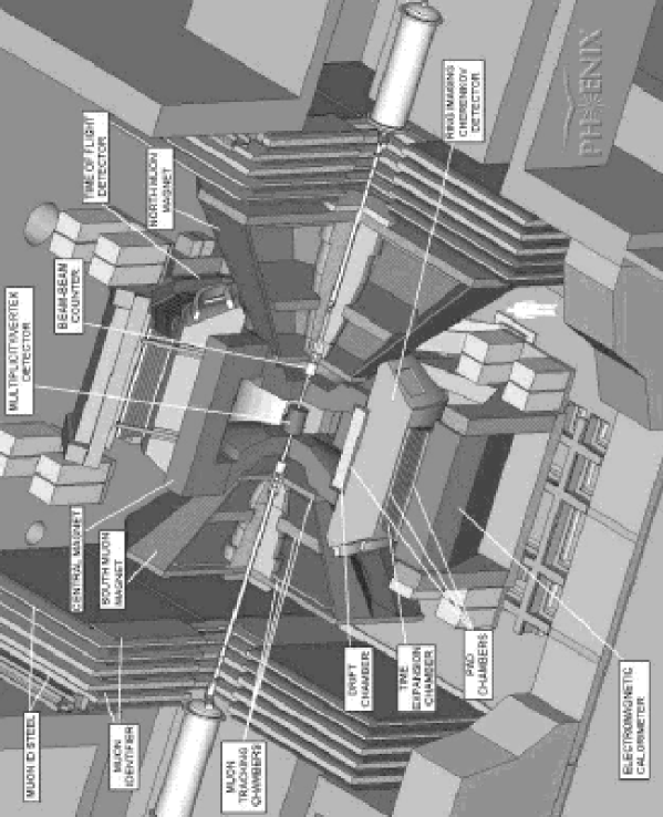
Figure 1: Layout of the PHENIX detector showing all four spectrometer arms within the PHENIX experimental hall. The collision point is in the center of the figure.

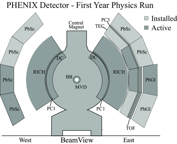
Figure 2: Schematic diagram of the PHENIX Central Arm Spectrometers. The abbreviations are defined in the text. The darker shading indicates which detectors were implemented for Run 2000.

2 The PHENIX Central Arm Spectrometers

In order to provide a spectrometer with optimized particle identification capabilities for various particle species, the central arm spectrometers, which each cover $\mathnormal{\pm}$0.35 in pseudorapidity ($\mathnormal{\eta}$) and span $90^{0}$ in azimuthal angle ($\mathnormal{\phi}$), necessarily contain many components. When there are differences in the two spectrometers, they will be referred to as the east and west arms. The positions of the detectors will be described in a coordinate system with the origin at the center of the central arm magnet with the z-axis along the beam. This section will briefly describe each component moving outwards radially from the beam pipe.

The innermost detector in each spectrometer is the drift chamber (DC) [2]. The drift chamber provides the primary vector and momentum measurement for charged particles traversing the spectrometers. The drift chamber consists of 40 planes of wires arranged in 80 drift cells placed cylindrically symmetric about the beam line. Each drift chamber spans $90^{0}$ in $\mathnormal{\phi}$, has a radial sensitive region from 2.02 to 2.46 meters, and covers -80 $<$ z $<$ +80 cm. The wire planes are placed in an X-U-V configuration in the following order (moving outward radially): 12 X planes (X1), 4 U planes (U1), 4 V planes (V1), 12 X planes (X2), 4 U planes (U2), and 4 V planes (V2). The U and V planes are tilted by a small $\mathnormal{\pm}5^{0}$ stereo angle to allow for full three-dimensional track reconstruction. The field wire design is such that the electron drift to each sense wire is only from one side, thus removing most left-right ambiguities everywhere except within 2 mm of the sense wire. The wires are divided electrically in the middle at $z=0$. The occupancy for a central RHIC Au+Au collision is about two hits per wire. The magnetic field bends particles in the x-y plane. Generally, the drift chamber active volume lies outside of the axial magnetic field, however there is a residual field within the volume that provides less than $1^{0}$ of deflection in the bend plane. There is no bending, to first order, in the non-bend plane, except for tracks very close to the magnet pole edges or at low momentum [3]. The deflection of the tracks is sufficiently low that the track model assumption can be straight line trajectories in both planes.

Attached to the back of the drift chamber, at an inner inscribed radius of 248 cm, is a single layer of pad chamber called PC1. This is a pixel-based detector [4, 5] with effective readout sizes of 8.45 mm in $z$ by 8.40 mm in the $x-y$ plane, providing three-dimensional space-point information for charged particles in the spectrometer.

Behind PC1 is a cylindrically shaped Ring Imaging Cherenkov Detector (RICH) [6, 7]. The RICH is the primary detector for electron identification in PHENIX. It is a threshold Cherenkov detector with a high angular segmentation to cope with the high particle density expected in the most violent collisions at RHIC. There are two identical RICH detectors, one in each PHENIX arm. Each RICH detector consists of a gas vessel, thin reflection mirrors, and photon detectors made up of arrays of photo-multiplier tubes (PMT’s). During Run 2000, $CO_{2}$ was used as the Cherenkov radiator. Pions below 4.9 GeV/c do not produce a signal in the RICH, while electrons above 18 MeV/c emit Cherenkov light in the gas radiator. The Cherenkov photons are reflected by the mirrors in the RICH, and are focused onto the photon detectors. A charged particle track is identified as an electron when a sufficient number of RICH PMT hits are associated with it.

On the west arm only, a second pixel pad chamber, named PC2, is located behind the RICH at an inner inscribed radius of 419 cm. This detector was not installed for Run 2000. PC2 has an effective readout size of 14.25 mm in $z$ by 13.553 mm in the $x-y$ plane.

On the east arm only, a Time Expansion Chamber (TEC) [8] is placed behind the RICH with a radial active area from 4.1 to 5.0 meters. One of the four installed TEC detector planes were instrumented for Run 2000 providing azimuthal coverage of $\mathnormal{\phi}$ = $45^{0}$. The TEC contains four planes of wire readout (expandable to six planes in the future). The wires are divided electrically at their center at z=0. The readout electronics consist of a 5-bit non-linear flash ADC. The TEC provides 2-dimensional tracking in the x-y plane, contributes to electron-pion discrimination via dE/dx measurements, and provides high momentum resolution for high $p_{t}$ particles. The TEC is located outside of the axial magnetic field, so a straight line track model assumption is valid for TEC track reconstruction.

Placed at an inner inscribed radius of 490 cm on each arm is a third layer of pixel pad chamber, called PC3, with an effective readout size of 16.7 mm in $z$ by 16.0 mm in the $x-y$ plane. Only the east arm of PC3 was installed for Run 2000.

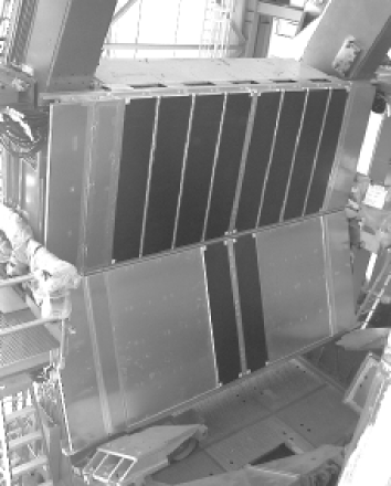
Figure 3: The TOF detector system mounted on the PHENIX East arm in the PHENIX experimental hall showing 10 panels of the detector.

Located on the east arm only is the time-of-flight detector (TOF) placed at an inner inscribed radius of 510 cm (between PC3 and the calorimeter) and spanning $30^{0}$ in $\mathnormal{\phi}$. The TOF detector, shown mounted on the east arm in Fig.  3, serves as the primary particle identification device for charged hadrons in PHENIX. The TOF wall is finely segmented in order to cope with the expected highest multiplicity events in central Au + Au collisions, which is about 1000 charged particles per unit rapidity. One TOF panel contains 96 plastic scintillation counters (Bicron BC404) with photomultiplier tubes (Hamamatsu R3478S) at both ends of the slat. A total of 10 TOF panels, 960 slats, and 1920 channels of PMT’s were installed for Run 2000. Each slat is oriented along the $r$-$\mathnormal{\phi}$ direction and provides timing as well as longitudinal position information of particles that hit the slat.

On the east arm only, placed behind the TOF detector, are two planar arrays of Lead-Glass calorimeters (PbGl) imported from the CERN SPS experiment WA98 [9], as were the TOF detectors. Behind PC3 on the remainder of the east arm lie two planar arrays of Lead-Scintillator calorimeters (PbSc) [10]. Both of these arrays span $45^{0}$ in $\mathnormal{\phi}$ on the east arm. Covering the full $90^{0}$ in $\mathnormal{\phi}$ on the west arm, and placed behind PC3, are four PbSc arrays. The calorimeters, collectively referred to as EMC, provide photon identification information, particle energy, and time-of-flight measurements.

Trigger, timing, and collision centrality information is provided by a set of detectors including a Beam-Beam Counter (BBC) [11], a pair of Zero-Degree Calorimeters (ZDC) [12, 13], and a Multiplicity Vertex Detector (MVD) [14]. The BBC consists of two identical sets of counters installed on both sides of the interaction point along the beam. Each counter is composed of 64 PMT’s equipped with a quartz Cherenkov radiator and covers the 3.0 $<\eta<$ 3.9 region with full azimuthal coverage. The ZDC’s are small transverse area hadron calorimeters which measure the energy of unbound neutrons in small forward cones ($\mathnormal{\theta}$ $<$ 2 mr) around each beam axis. One ZDC is located on either side of the interaction region and consists of 3 modules, each with a depth of 2 hadronic interaction lengths and read out by a single PMT. Both time and amplitude are digitized for each of the 3 PMT’s as well as an analog sum of the PMT’s for each ZDC.

The MVD is a highly segmented silicon strip and pad detector. It is designed to measure and trigger on the number of charged particles, as well as to measure the collision vertex with high accuracy. The detector has a large pseudorapidity coverage (approximately -2.64 $<\eta<$ 2.64) and full azimuthal coverage, making it possible to study charged particle production as a function of $\eta$ and $\phi$ on an event-by-event basis. The detector is composed of two parts: two concentric barrels, or shells, spanning -32 $<z<$ 32 cm, and two endcaps at z=$\mathnormal{\pm}$35 cm. Each barrel shell consists of six rows of detectors, where each row is formed by 12 panels of silicon strip detectors with a 200 $\mu m$ pitch. The disk-shaped endcap sections are each composed of six silicon pad wafers each segmented into 252 pads. When fully instrumented, about 35,000 channels will be read out from the MVD.

3 Beam-Beam Counters and Zero Degree Calorimeters

The Beam-Beam Counters (BBC) and Zero Degree Calorimeters (ZDC) are designed to define the start timing of the nuclear interaction for time-of-flight measurements, to provide the trigger signal of the nuclear interaction, and to provide a coarse measurement of the collision vertex along the beam axis. The following equations are used to calculate the start timing ($T_{0}$) and the vertex position along the beam axis ($Z_{vertex}$) for both detectors: $T_{0}=(T_{1}+T_{2})/2$ and $Z_{vertex}=(T_{1}-T_{2})/2c$, where $T_{1}$ and $T_{2}$ are the average hit timing for each set of BBC counters, and $c$ is the velocity of light.

The average hit timing in each BBC set is defined by taking a truncated average of the timing over the PMT’s that have a hit (defined as a PMT with a valid timing signal) out of the 64 possible PMT’s. In the case that there is no peak structure in the hit timing distribution in either BBC set due to low particle multiplicity, the arrival times of the first leading particle from the beam collisions are used as the hit timing value.

The ZDC pulse height is converted to hadronic energy equivalent using peripheral interactions with low neutron multiplicity in the ZDC where single- and double-neutron peaks are clearly seen. The fitted single-neutron peak position is equivalent to 65 AGeV per beam for Run 2000. This fit procedure was performed using an analog sum channel since pedestal offset corrections are reduced in this channel. The offset arises because the analog-to-digital converters used for the BBC and ZDC are self-gating, so a minimum signal must be present to start the digitization.

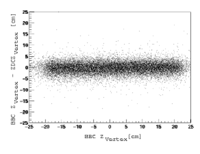
Figure 4: The difference in the measured BBC and ZDC $Z_{vertex}$ positions as a function of the measured BBC $Z_{vertex}$ position from the Run 2000 data.

The time-of-flight to the ZDC was calculated using the PMT digitized times after correcting for pulse height slewing via a look-up table. The typical signal rise-time is 2 nsec. The time digitizer least-count scale was calibrated with standard delay cables. The resulting time measurements are used to calculate $T_{0}$ and $Z_{vertex}$ as outlined above using a C++ class whose data members are stored for each event for both the BBC and ZDC. Fig.  4 plots the difference between the measured ZDC and BBC vertex positions as a function of the BBC vertex position. The resolution in the difference is 2.0 cm, which is dominated by the contribution from the ZDC time resolution.

4 Multiplicity Vertex Detector

The Multiplicity Vertex Detector (MVD) is designed to measure and trigger on the number of charged particles produced in high multiplicity events in Au+Au collisions and to measure the collision vertex with high accuracy. Vertex finding is performed by the MVD barrel section where the hit information from the two shells of detectors can be combined and projected onto the z-axis. Multiplicity measurements are performed by both the barrel and pad sections. For a vertex at the center of the MVD ($z=0$), the inner shell covers the range -2.55 $<\eta<$ 2.55 and the Si pad detectors cover the range 1.79 $<|\eta|<$ 2.64 at each end of the detector. Both the inner shell and the pads have complete azimuthal coverage.

The MVD event processing, written in C++, is handled by an MVD event reconstruction object, which is created and evaluated for each event by the main MVD reconstruction module. The event reconstruction object contains data members holding the hit information for each event and the final vertex and $dN/d\eta$ results. The content of these data members are evaluated by a call to the internal event processing method. Strips, pads, hit clusters, and the vertex are treated as individual objects for the given event. The content of the cluster objects are generated from the strip objects. Strip, pad, and cluster objects are accessed by a vertex object class which holds the methods containing the main reconstruction algorithms.

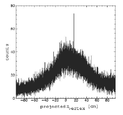
Figure 5: MVD vertex finding histogram for the pseudo-tracking method using simulated central HIJING Au+Au events. The narrow peak defines the vertex.

Two different algorithms are used to find the vertex position. The first algorithm is denoted the pseudo-tracking method. This vertex algorithm takes each pair of clusters (where a cluster is a group of adjacent channels in the same row, shell, and panel of the MVD which all have signals above a threshold) in the inner and outer shells and treats every combination in the same row of the MVD barrel as a potential track. This combination of track candidates is projected back to the beam axis to determine the vertex expected for a track which hit these two locations. For each of these possible vertex locations, a channel in a histogram is incremented. Most pairs of hits do not correspond to a real track. However, when all pairs are considered, the true vertex location appears more frequently than the other locations. A clear peak appears in the histogram corresponding to the vertex position, as shown in Fig.  5 from simulated central Au+Au events using the HIJING event generator [15]. When this algorithm finds the correct vertex location, it is correct within a standard deviation, $\sigma$, of about 190 $\mu$m for simulated central events and 224 $\mu$m for simulated minimum bias events. At high occupancy (around 45% in the inner shell) this method becomes more inefficient (less than 98%) and a different approach must be used.

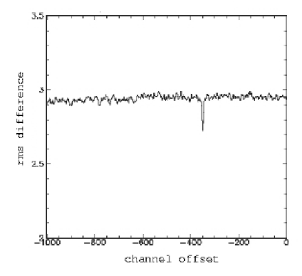
Figure 6: MVD vertex finding histogram for the correlation method using simulated central HIJING Au+Au events. The narrow dip defines the vertex.

The alternative vertex algorithm, used for high multiplicity events, is the correlation method. Unlike the pseudo-tracking method, the correlation method makes use of the ADC information from the individual channels. The algorithm is based upon the assumption that the pattern of energy loss per channel in the inner and outer shells of the MVD are similar. The pattern of ADC values in the outer shell of the MVD is scaled down by the ratio of the inner-to-outer shell radius and stored in an array. The scaled pattern yields an offset proportional to the vertex location when compared to the unscaled inner shell pattern. By finding the value of the offset which makes the two patterns most similar, the vertex position is found. A histogram which plots the difference between the pattern of hits in the inner and outer shells will show a sharp minimum which corresponds to the location of the vertex, as shown in Fig.  6 from central HIJING Au+Au events. This method gives the correct vertex with a standard deviation of 233 $\mu$m for simulated central events and 250 $\mu$m for simulated minimum bias events with an efficiency greater than 99% for inner shell occupancies above 5%.

The algorithms for calculating $dN/d\eta$ are different in the MVD barrel section and endcap sections. In the MVD barrel, only the inner shell is used. In central Au+Au collisions, the occupancy in the inner shell is high [14], therefore the algorithm makes no attempt to find individual hits. Instead, the barrel is divided into groups of 64 adjacent strips which are in the same row (azimuthal segment). For each of these groups of channels, a $dN/d\eta$ value is calculated as follows: the total ADC value for all channels in this group is added up, the range of pseudorapidity ($\Delta\eta$) is calculated, the pseudorapidity at the center of the group of strips is calculated, a geometric correction (for non-normal incidence) is applied, the number of particles is estimated by dividing the corrected ADC signal by the ADC signal expected for a minimum ionizing particle (mip), and finally $dN/d\eta$ is estimated as the number of particles divided by $\Delta\eta$. The average $dN/d\eta$ for a set of events is calculated by taking the average in each bin of $\eta$.

In order to calculate $dN/d\eta$ from the MVD pads, the algorithm assumes that a single particle hits only one pad. The occupancy of the pad detectors is around 15-20% for central events. The algorithm estimates the number of particles associated with the observed ADC value in an individual pad using an ADC distribution which is taken from the distribution corresponding to the ADC response expected for a single particle at normal incident angle in low multiplicity events, and the occupancy of the pad detector. The algorithm does not associate an integer number of particles with each hit. Instead a mean number of particles which would be associated with a given ADC channel is calculated. This number can then be converted into a $dN/d\eta$ value using the vertex location and the pad geometry.

5 Pad Chambers

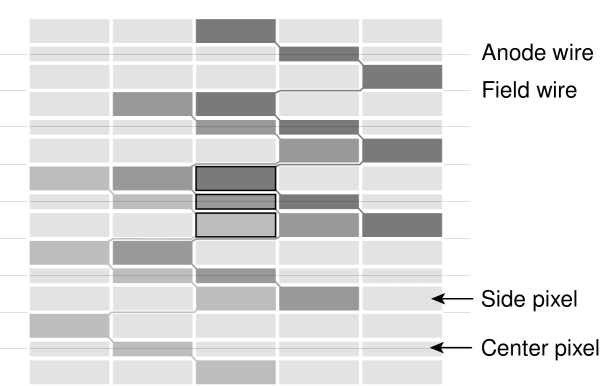
Figure 7: The pad chamber pixel pattern. The three pixels form a cell at the center of the figure. Nine connected pixels form a pad.

A new pad geometry for cathode readout of MWPC’s was designed for the PHENIX pad chambers [5, 16]. The basic component in this geometry is a pad consisting of nine smaller connected copper electrodes, called pixels (Fig.  7). The pad is read out by a single preamplifier and discriminator. The pads are interleaved in a repeated pattern. The area defined by three adjacent pixels belonging to three different pads is called a cell. This arrangement saves a factor of three in the number of readout channels with marginal loss of performance.

Pad chamber information, which is stored in the PHENIX Objectivity database, can be separated into three different groups: geometry, high voltage and electronics. All groups are accessed via object-oriented classes in the offline analysis, using time stamps as the primary key. The geometry group holds information on the geometry parameters of the chambers themselves, e.g. wire-spacing, as well as survey information, while the high voltage group keeps track of when trips have occurred. The electronics group contains threshold and gain calibrations, as well as information on where hot or inactive channels are located.

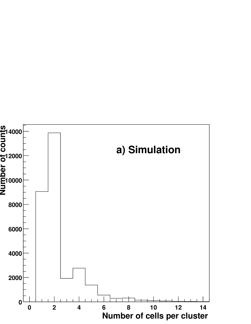
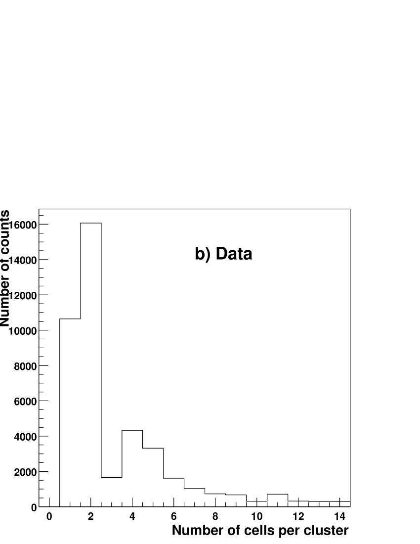
Figure 8: The distribution of the number of cells per cluster in PC3 from a) simulation and b) data.

The list of fired pads from an event is read by the hit reconstruction algorithm, which first translates it into a list of fired cells. The limit on the number of allowed inactive or hot pads in a cell is an input parameter whose default value is one, i.e. at least two out of three pixels in a cell have to be part of alive channels. From the cell list, cluster objects are built for each chamber by identifying all neighboring cells. The size of each cluster is checked against a pre-defined table to estimate the number of traversing particles that created the cluster. The default settings of this table were determined from simulations [16]. If the number of particles in a cluster is considered to be greater than one, the cluster will be recursively split depending on its shape until only one-particle clusters remain. Once a cluster created by a single particle has been extracted, the average hit position is calculated by averaging over the coordinates of the cells in the cluster. The entire procedure is repeated until the list of fired cells is empty.

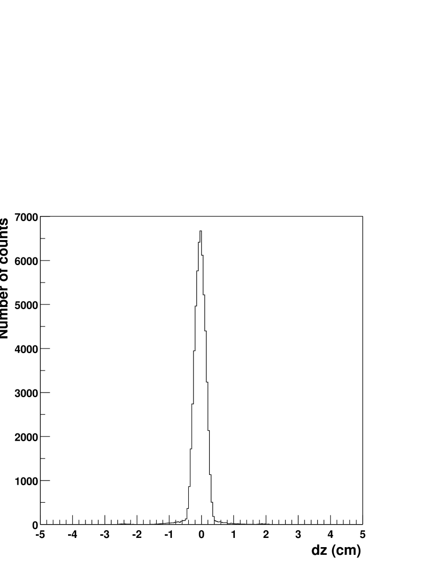
Figure 9: The simulated position resolution along the wire (left panel) and across the wire (right panel) in PC1.

In order to determine the reconstruction efficiency, a pad chamber response simulator, which simulates which pads fired in an event, is utilized. Given the coordinates of a particle entering and exiting the pad chamber, the location of the avalanche along the closest wire is calculated. The particle may also give rise to additional avalanches on neighbouring wires. The total avalanche charge is obtained from a Landau distribution. The induced charge distribution on the pad cathode plane is then calculated from an empirical formula [17, 18]. Finally, when all particles of the event are processed, noise charge drawn from a normal distribution is added to each pad in the chamber. If the total collected charge on a pad exceeds the threshold value, the pad is registered as fired. The thresholds used in the simulation were set to match the cluster sizes (Fig.  8) and the very high efficiency of the real chambers.

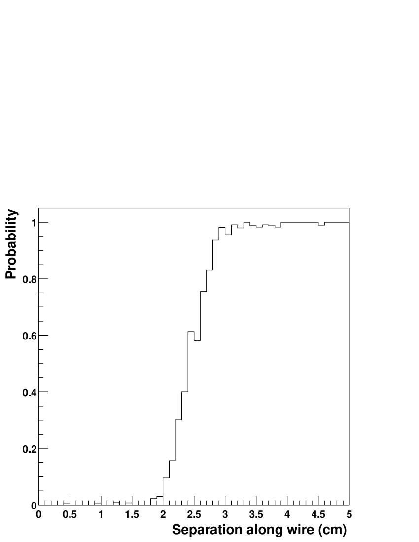
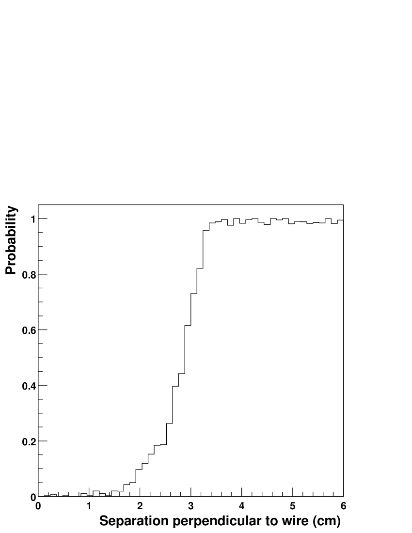
Figure 10: The probability to reconstruct two simulated particles as two separate hits as a function of the separation of the particles in PC1 both along the wire (left panel) and across the wire (right panel).

Table 1: Pad chamber position and two-track resolutions.

Simulation Results	PC1	PC2	PC3
Position resolution along wire [mm]	$1.6$	$2.7$	$3.2$
Position resolution across wire [mm]	$2.3$	$4.0$	$4.8$
Two-track resolution along wire [cm]	$2.4$	$4.0$	$5.0$
Two-track resolution across wire [cm]	$2.9$	$4.6$	$5.3$

The position resolutions, presented in Table 1, are determined by comparing the reconstructed hit positions with the positions where the original GEANT [19] particles passed through the chambers. The position resolutions for PC1 are shown in Fig.  9. By simulating minimum ionizing particle pairs with small separation between them, the probability for resolving the nearby tracks was calculated. Shown in Fig.  10 is the two-track resolution along and perpendicular to the wires for the PC1 chamber. The resolution is defined as the distance where 50% of the tracks are separated by the reconstruction. The system can be optimized for two-track resolution at the expense of an increased number of ghost hits (due to falsely split clusters) or loss of single track efficiency by operating at lower sensitivity (leading to reduced cluster sizes). The study presented here results in a negligible number of ghosts. While the detection efficiency as measured with cosmic rays is greater than 99.5%, the reconstruction efficiency is slightly lower as determined by projecting reconstructed drift chamber tracks from minimum bias data into PC1. This results in a reconstruction efficiency calculated to be better than 98%, as expected from the pad chamber simulation.

6 Drift Chamber

Track reconstruction within the drift chamber is performed using a combinatorial Hough transform (CHT) technique [20, 21]. In this technique, the drift chamber hits are mapped pair-wise into a feature space defined by the polar angle at the intersection of the track with a reference radius near the mid-point of the drift chamber, $\mathnormal{\phi}$, and the inclination of the track at that point, $\mathnormal{\alpha}$. The $\mathnormal{\alpha}$ variable is proportional to the inverse of the transverse momentum, thus facilitating limited searches for specific momentum ranges and providing an initial guess for the momentum reconstruction procedure. Fig.  11 provides a schematic illustration of these variables.

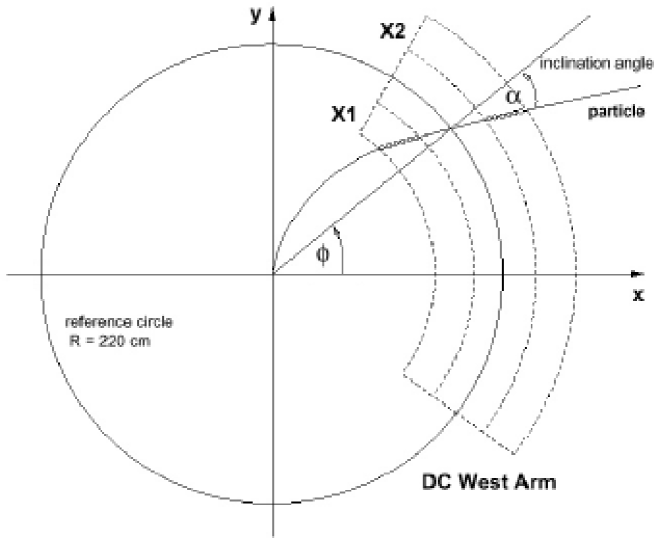
Figure 11: Illustration of the Hough transform parameters for drift chamber track reconstruction. The outline shows the drift chamber active volume. The circles represent drift chamber hits along the particle trajectory.

This coordinate mapping results in a gain effect that greatly enhances the peak-to-background ratio in the feature space. If n is the number of points on the track, the nominal peak height is $n(n-1)/2$. In order to minimize computation time, $\mathnormal{\alpha}$ and $\mathnormal{\phi}$ were only calculated for hit pairs separated in azimuthal angle by physically reasonable amounts corresponding to $p_{t}$ = 150 MeV/c, comparable to the natural resolution of the spectrometer. Fig.  12 shows an example of a region of the drift chamber hits and the associated feature space from a simulated HIJING central RHIC Au+Au collision. In order to reconstruct tracks in regions where some wires have been removed for internal supports, the algorithm first looks for tracks that traverse both the X1 and X2 wire regions, then it looks for the remaining tracks that traverse the X1 or X2 regions only.

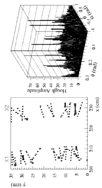
Figure 12: The left panel shows simulated hits from a central Au+Au collision for a small physical region of the drift chamber. The right panel shows the Hough transform feature space for this region. Tracks appear as peaks in this plot.

After reconstructing a track in the magnetic field bend plane, the direction of the track is specified by $\mathnormal{\phi}$ and $\mathnormal{\alpha}$. Track reconstruction in the non-bend plane is first attempted by integrating information from PC1 reconstructed clusters, which contain $z$ information with a resolution of 1.89 mm. A straight line projection of the bend-plane track is made to the PC1 detector and a road is defined about that projection. If there is an unambiguous PC1 association, the non-bend vector is defined by the PC1 cluster and the $z$-coordinate of the event vertex. This assumption is not valid for secondary tracks, but those cases are later examined during momentum reconstruction. If there is no PC1 cluster association, or if there are multiple PC1 association solutions, the non-bend vector is determined from the stereo wires. For this procedure, a plane, called the X-plane, is defined by $\mathnormal{\phi}$ and $\mathnormal{\alpha}$, but extending in $z$. The path of the track trajectory through the X-plane is a straight line and is determined by including the information measured by the stereo wires. To do this, all drift chamber hits are defined as lines in physical space parallel to the anode wire and perpendicular to the drift direction. All stereo wire hit lines are intersected with the X-plane with the intersections belonging to the track defining a line in the X-plane. Again, a Hough transform is used to extract these intersections by using the $z$ coordinate at which the track crosses the reference radius, $zed$, and the polar angle at that point, $\mathnormal{\phi}$. Since the X-plane is defined by a single track, a unique solution in this space is extracted.

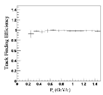
Figure 13: The reconstruction efficiency in HIJING-simulated central Au+Au events as a function of the transverse momentum of the track.

The method of determining the drift chamber track reconstruction efficiency will be discussed in more detail in Section 12. Using this method, the drift chamber tracking efficiency as a function of transverse momentum is shown in Fig.  13 with less than 1% spurious (ghost) tracks. The resulting spatial resolution of the tracks is comparable to the single-hit resolution of the detector.

7 Time Expansion Chamber

Track reconstruction in the Time Expansion Chamber (TEC) is performed using a Combinatorial Hough Transform method using the identical variables, $\mathnormal{\alpha}$ and $\mathnormal{\phi}$, and with an identical method for track reconstruction in the magnetic field bend plane as the drift chamber track reconstruction.

A detailed simulation of the TEC detector response is used to determine the TEC tracking efficiency. This simulation calculates the average number of primary ion collisions for each track section that traverses a single drift cell [22]. Fluctuations of the number of primary collisions are modelled by Poisson statistics [23]. Secondary ionization is calculated by generating a spectrum of $\mathnormal{\delta}$ electrons [23]. The total number of primary and secondary ion pairs are calculated and the distance of the electron cluster to the wire, along with the drift time, are calculated assuming a straight line drift. Gas gain fluctuations are simulated using a polya distribution [24]. After the addition of noise, and the addition of the electronics shaping time response, the charge collected on the wire as a function of time bin is calculated. The charge is finally converted into FADC channels for each track. The final FADC contents are obtained by summing the contributions from all charged tracks in the event. The track reconstruction efficiency is determined by embedding individual simulated tracks processed through the response simulation into a real data event, reconstructing the resulting merged event and determining how many of the embedded tracks are correctly reconstructed. The reconstruction efficiency is shown as a function of the charged track multiplicity in the TEC in the left panel of Fig.  14. The spatial resolution of reconstructed tracks in the TEC, shown in the right panel of Fig.  14, is determined directly from data taken in Run 2000 by comparing the residuals of tracks reconstructed independently in alternating planes of the TEC and fitting them to a Gaussian curve. The resulting resolution, also confirmed within the simulation procedure, is determined to be 380 $\mu$m.

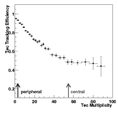
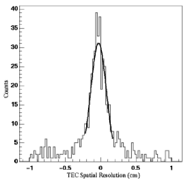
Figure 14: The TEC track reconstruction efficiency as a function of the TEC charged track multiplicity obtained by evaluating simulated tracks embedded in real data events (left panel), and the spatial resolution of 380 $\mu$m of the TEC based upon data taken in Run 2000 (right panel). The arrows on the left panel correspond to the 5% most central, and the 60-80% peripheral events in the Au+Au collisions.

8 Electromagnetic Calorimeters

Pattern recognition in both the PbSc and PbGl Electromagnetic Calorimeters (EMC) includes single electromagnetic shower identification including calculation of the shower position, energy, time-of-flight, overlapping shower separation, and hadronic shower rejection. The technique is based upon matching energy- and impact-angle-dependent descriptions of the projected electromagnetic shower shape as measured in a test beam of electrons in the momentum range 0.3-5.0 GeV/c [26] and reproduced in a detailed GEANT simulation of the detector response. An illustration of the shape of a shower is shown in Fig.  15 for a particle impact orthogonal to, and at a $20^{0}$ impact angle to, the calorimeter surface.

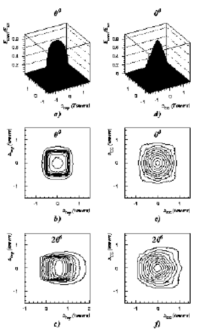
Figure 15: Energy deposited in a PbSc calorimeter tower as a function of the distance between the tower center and the impact point (left panels), the tower center and the shower center-of-gravity (right panels); a),b),d) and e) are for orthogonal impact; c) and f) are for a $20^{0}$ impact angle.

The shower reconstruction algorithm includes two steps. First, a cluster search is performed. The cluster is defined as a contiguous group of calorimeter towers with measured energies above a certain threshold. At this point, the clusters are considered to be totally independent. Second, the clusters are split into subclusters associated with local maxima. A local maximum is defined as a tower which has a deposited energy in excess of the energies measured in any of the 8 surrounding towers. A subcluster (peak region) is formed from the towers of the cluster sharing the energy in each tower among photons located in each peak region. Here, an iterative procedure based on a parameterized shower profile is used [25]. Each subcluster is assigned a $\chi^{2}$ value for shower identification purposes.

The simplest algorithm for determining the particle position in a cellular calorimeter is to measure the center-of-gravity of the shower, $X_{CG}$:

$$X_{CG}\equiv\frac{\sum{x_{i}E_{i}}}{\sum{E_{i}}},$$ (1)

where $x_{i}$ is the $x$-coordinate of the center of tower $i$, and $E_{i}$ is the energy deposited in the tower. For electron and photon position reconstruction, a parametrization of the shower center-of-gravity in units of tower width is applied [28]:

$$X_{CG}=\frac{1}{2}\frac{sinh(\frac{X_{imp}+\Delta-\delta}{b})}{sinh(1/2b)}+\delta;|X_{imp}+\Delta-\delta|\leq\frac{1}{2}.$$ (2)

where $X_{imp}$ is the particle impact point, $b$ is the shower cross-sectional width, $\Delta$ is the mean displacement of the calculated shower center-of-gravity from the impact point $X_{imp}$, and $\delta$ is a phase shift related to the skewed shape of the shower projection. All of these parameters ( $b$, $\Delta$, and $\delta$) are parameterized as a function of the incident particle energy, $E$, and angle of incidence, $\theta$. $\Delta$ is given by

$$\Delta=L_{eff}\cdot sin(\theta),$$

where $L_{eff}$ is the effective depth of the shower penetration in the calorimeter as determined by the position of the cascade-curve median in the longitudinal direction ($\propto ln(E)$) [29]. The value of $b$ is given by

$$b=b_{0}+b_{1}(E)sin^{2}(\theta),$$

where $b_{0}$ is a constant and $b_{1}(E)\propto ln(E)$. $\delta$ is found to be essentially energy-independent and can be parameterized as a function of the impact angle only. Finally, the position of the particle impact on the calorimeter surface, $X_{imp}$, is calculated according to the formula obtained by inverting Equation (2):

$$X_{imp}=b\cdot arcsinh[2\cdot(X_{CG}-\delta)\cdot sinh(1/2b)]-\Delta+\delta,$$

$$|X_{CG}-\delta|\leq\frac{1}{2}.$$

The calorimeter position resolution is well described by [27, 28]:

$$\sigma_{X}(E,\theta)=\sigma_{X}(E,0^{0})\oplus(d\cdot sin(\theta)),$$

where $\sigma_{X}(E,0^{0})$ is the position resolution for an orthogonal incidence. The second term in this parametrization describes the contribution of the longitudinal shower fluctuations on the projection to the calorimeter surface. The value of $d$ is $0.8X_{0}$, where $X_{0}$ is the radiation length in the calorimeter module. Using the electron test beam, a position resolution of $5.7mm/\sqrt{E(GeV)}+1.6mm$ was achieved.

A number of factors are taken into account when reconstructing the photon and electron energy in the calorimeters: the longitudinal energy leakage, the light attenuation in the calorimeter module, the response dependence on the particle impact position, and the shower overlaps in the high multiplicity environment, some of which will be discussed here. The nonlinearity of photon and electron energy measurements in the calorimeters is primarily connected with light attenuation in a calorimeter module. This is well described by the expression $E_{EMC}/E\approx E^{\frac{X_{0}}{\lambda_{att}}}$, where $E_{EMC}$ is the energy measured in the calorimeter, and $E$ is the actual photon or electron energy in GeV.

In a high multiplicity environment, shower overlaps can seriously affect the electromagnetic shower energy measurements, thus degrading the energy resolution and inducing systematic shifts in the measurement. For a tower energy threshold of 3 MeV, the mean cluster size in the PbSc calorimeter initiated by a 0.5 GeV (4 GeV) photon is 7 (19) towers. The larger the cluster size, the higher the probability for an overlap. However, the shower size can be reduced to 4-5 towers in the shower core. Towers belonging to the shower core are defined using a parameterized shower profile:

$$r=\frac{E_{i}^{pred}}{E}<\epsilon,$$

where $r$ is the contribution of the tower to the total shower energy $E$, and $E_{i}^{pred}$ is the predicted energy deposited in the tower. The $\epsilon=0.02$ parameter is chosen in order to have as few towers in a cluster as possible while keeping the energy resolution on the same level. The shower core defined in this manner contains about $92\%$ of the total shower energy, dropping to $90\%$ for a $20^{0}$ impact angle. Using the shower core for energy measurements introduces an additional constant term of about $2\%$ in the energy resolution, which slightly worsens the energy measurements of isolated photons and electrons, but helps to considerably improve the energy measurements in the high multiplicity environment, where an energy resolution for the PbSc calorimeter of $8.2\%/\sqrt{E(GeV)}\oplus 1.9\%$ was achieved in electron test beams at the BNL AGS and the CERN SPS [26].

The time-of-flight (TOF) information provided by the calorimeters (using the BBC as the start counter) is a useful tool for particle identification. This helps by enhancing the $e/\pi$ separation at low momenta ($<0.8$ GeV/c), where the energy-to-momentum comparison, as well as the shower profile analysis, lose effectiveness for $e/\pi$ discrimination. In addition, this is the primary tool for identifying neutral hadrons, which are a major source of background in the photon spectrum in the energy region of approximately 1 to 3 GeV. Also, the magnet poles and structural elements of the detectors in front of the calorimeter are sources of non-vertex photons, part of which ($\sim 15$%) can be rejected using the TOF information. Finally, in the case of high multiplicity events, requiring consistency of the TOF values measured in the different towers within the same cluster can help to identify accidental shower overlaps. Several corrections are applied to measure the TOF, including slewing corrections and flight path corrections based upon the collision vertex, after which a resolution of better than 700 psec for the PbSc calorimeter was achieved.

9 Ring Imaging Cherenkov Detector

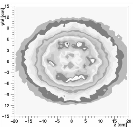
Figure 16: The distribution of hit PMT’s around the projected ray from a reconstructed track in zero-field runs after the geometry calibration.

Electron identification using the Ring Imaging Cherenkov Detector (RICH) is performed with two C++ classes. The first class handles the geometry of the RICH detector by modelling the position, shape, and orientation of the 96 mirror panels and the position of the 5120 PMT’s in the RICH detector. This class also handles all optical tracing calculations. The second class uses the geometry class and performs the electron identification. The electron identification class accepts a previously reconstructed track and searches for RICH PMT’s that can be associated with the track. This is done by first reflecting the track about the RICH mirror as if it were a light ray, and then projecting the reflected track onto the RICH PMT array. If the track is an electron, the reflected ray should be projected to the center of a ring formed by hit PMT’s. The number of hit PMT’s within a tight association radius from the projected track is counted and the number of photo-electrons measured in the PMT’s in the association radius is summed. In addition, a quality factor based upon the position of the associated hits and the position of the projected track is calculated. All of these quantities are then used to separate electron tracks from the hadron background.

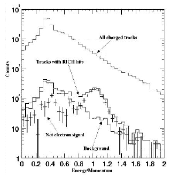
Figure 17: The electron signal observed in PHENIX. The highest histogram is the distribution of the energy and momentum ratio of all charged tracks in $0.8<p_{t}<0.9$ GeV/c. The middle histogram is the one with the RICH hits. The lowest histogram is the distribution of a random background estimated from the data. The crosses are the difference of the middle and the lowest, resulting in the net electron signal. The electron signal below $E/p<0.8$ are caused by electrons from photon conversions far from the beam pipe.

The gain of the RICH PMT’s is determined from the pulse height of the single photo-electron peak in the data. The geometry of the mirror system and the optics are calibrated from the data using zero magnetic field runs. In these runs, charged particle tracks are reconstructed as a straight line connecting the event vertex (determined by the BBC), the PC1 hit position, and the PC3 (or EMCAL) hit positions. The orientation of the mirror panels in the geometry class are then adjusted so that the projection point of the track reflected by the mirrors points to the center of the Cherenkov rings recorded in the PMT array. Fig.  16 shows the distribution of the hit PMT’s around the projected ray after the geometry calibration.

The hadron rejection factor provided by the RICH strongly depends upon the multiplicity of the event. From data taken with a test beam with a small proto-type of the RICH detector, it was shown that the RICH detector can provide a pion rejection factor better than $10^{4}$ with an electron efficiency close to 100%. However, in high multiplicity events, the electron-pion separation is reduced since a hadron track can be associated with a RICH hit produced by background electron tracks, resulting in a track that is mis-identified as an electron. The pion rejection factor in most central Au+Au collisions was determined to be on the order of several hundred with an electron efficiency of $\sim 80\%$. Fig.  17 illustrates electron identification using the RICH detector. In this figure, the ratio of the energy (measured by the calorimeters) and the momentum of the charged tracks in the $p_{t}$ range $0.8<p_{t}<0.9$ GeV/c are plotted. For all charged tracks, the $E/p$ ratio has a mip peak at $E/p\sim 0.3$ on a broad distribution caused by hadronic interactions. When RICH hits are required, a clear peak appears at $E/p=1.0$, which is the electron signal. The background due to random associations of the RICH and the track is estimated, and also shown in Fig.  17.

10 Time-Of-Flight Detector

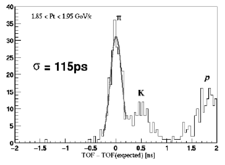
Figure 18: The time-of-flight resolution in the transverse momentum range $1.85<p_{t}<1.95$ GeV/c for positively charged pions. An overall time-of-flight resolution of 115 ps is achieved.

Prior to the application of the Time-Of-Flight detector (TOF) for particle identification, the flight time of a particle impacting the TOF is determined by taking the average of the measured stop time values at both ends of the hit PMT after subtraction of the start timing provided by the BBC. The pulse height information from the PMT’s is used to reconstruct the hit position by calculating the center-of-gravity of the pulse heights from each end of the slat after applying timing calibrations, gain calibrations, geometrical alignment corrections, and pulse-height-dependent timing, or slewing effect, corrections.

For TOF event reconstruction, four distinct C++ classes are used. The first class defines an address object, which provides the mapping between the actual read-out channel number of the Front End electronics Module (FEM) and a sequential slat identification number. The second class defines a geometry object, which handles the conversion from the slat identification number to the geometrical hit position of the particle within the PHENIX coordinate system. The third class defines a calibration object, which deals with all of the calibration parameters used for event reconstruction for the TOF system, such as the slat-by-slat timing offset, the position offset, and the PMT gain. Finally, the address, geometry, and calibration objects are accessed within a TOF reconstruction object within which the energy loss in the scintillators and the hit positions are reconstructed.

During Run 2000, the TOF detector timing offset was calibrated on a slat-by-slat basis using reconstructed track information. An overall time-of-flight resolution of $\sim$110-120 ps is achieved by selecting pions at high momentum and comparing their time-of-flight to that expected from a $v=c$ particle with a linear trajectory originating at the event vertex, as shown in Fig.  18 after corrections for the slewing effect and timing drift during the run. The method of particle identification using the TOF detector will be discussed in Section 13.

11 Momentum Reconstruction and the Track Model

Due to the complicated, non-uniform shape of the focusing magnetic field along the flight path of charged particles traversing the PHENIX central arm spectrometers, an analytic solution for the momentum of the particles cannot be determined. Therefore, other approaches such as look-up tables, must be used [3]. For Run 2000, a four-dimensional field-integral grid was constructed for momentum reconstruction using the drift chamber and for track model definition within the entire radial extent of the central arms. The variables in the field-integral grid are the $z$ coordinate of the event vertex; the polar angle, $\theta_{0}$, of the particle at the vertex; the total momentum of the particle, $p$; and the radius, $r$, at which the field-integral $f(p,r,\theta_{0},z)$ is calculated. The field-integral grid is generated by explicitly swimming particles through the measured magnetic field map and numerically integrating to obtain $f(p,r,\theta_{0},z)$ for each grid point.

An iterative procedure is used to reconstruct the momentum of a reconstructed track, utilizing the fact that $f(p,r,\theta_{0},z)$ varies linearly with the $\phi$ angle of the track at a given radius. This can be expressed as $\phi=\phi_{0}+q\cdot f(p,r,\theta_{0},z)/p$. Each track is assumed to be a primary track originating from the event vertex as determined by the BBC. An initial estimate of the track momentum and charge is made from the reconstructed bend angle, $\alpha$, of the track in the drift chamber. The measured polar angle, $\theta$, of the track in the non-bend plane at the drift chamber reference radius is used as an initial estimate of $\theta_{0}$. Then, using the radial position of each reconstructed hit associated to the track, a four-dimensional polynomial interpolation of the field-integral grid is performed to extract a value of $f(p,r,\theta_{0},z)$ for the drift chamber hit. Once this is done for all hits, a robust fit in $\phi$ and $f(p,r,\theta_{0},z)$ is performed to extract the quantities $\phi_{0}$ and $q$/$p$ for the track. The extracted values are then fed back into the above equation. The initial polar angle, $\theta_{0}$, is also determined using an iterative procedure using the equation $\theta=\theta_{0}+\delta(p,r=R,\theta_{0},z)-g(p,r=R,\theta_{0},z)/p$ where $\delta$ is the bend angle of the particle trajectory relative to the straight-line trajectory of an infinite-momentum particle. Typically, less than four iterations are necessary for convergence on these quantities.

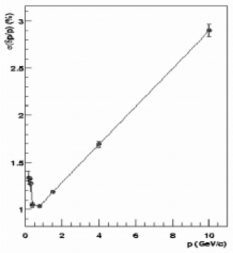
Figure 19: Momentum resolution as a function of momentum from simulated single particle events.

This procedure has an additional advantage in that it can be used to define the shape of the track within the central arm magnetic field, which can be then be used to determine the track intersections with each detector in order to facilitate inter-detector hit association as described in the next section. This is done by storing the coordinates of the particle in radial steps as additional entries (but not keys) in the field-integral grid. Line segments connecting the interpolated grid coordinates for a track are intersected with the geometry objects describing the position of each detector in order to estimate the projection of the track on each detector. These projections are used as a seed for inter-detector hit association. Finally, the length of the interpolated line segments from the event vertex to a given detector can be summed in order to provide an estimate of the flight distance of the particle to that detector. This quantity is used to facilitate particle identification using the TOF.

The momentum reconstruction resolution is determined by generating simulated muons (which will not decay as they traverse the spectrometer) with momentum $p_{gen}$ and event vertices ranging from $-40<z<40$ cm. A complete GEANT and detailed detector response simulation on each track is performed to obtain the detector hits as they would appear in the data, after which the reconstruction is run in the same manner as for data, producing a reconstructed momentum, $p_{rec}$. The quantity $|p_{rec}-p_{gen}|/p_{gen}$ (in percent) is shown in Fig.  19. Multiple scattering dominates the resolution at low momenta, while detector resolution determines the resolution at higher momenta. In addition, the momentum resolution is not multiplicity-dependent, as observed by generating the same plot using central Au+Au HIJING events.

12 Inter-Detector Association

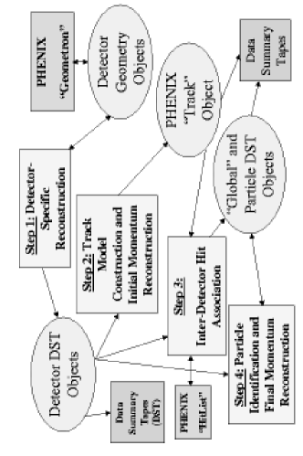
Figure 20: Illustration of the object-oriented approach to inter-detector association in PHENIX.

This section will address the methods and algorithms used for inter-detector association. The general object-oriented flowchart used for inter-detector, or global, reconstruction is shown in Fig.  20. All stages of the event reconstruction query the geometry information for the spectrometer, which is stored as Detector Geometry Objects. Geometry interactions (intersections, transformations, etc.) are handled either within a specific geometry object type, or within a C++ singleton class called the Geometron. The output of detector-specific reconstruction are stored in objects containing the hit and track information, which are stored in the Data Summary Tapes (DST) created after each reconstruction pass. The anchor of inter-detector hit association is the track model object, which is discussed further below. Once a track model object is created, its methods are used to perform hit association in addition to momentum reconstruction with the assumption that the particle is a pion. The resulting association and kinematics information is stored in distinct objects (and in the DSTs), which are then fed into the particle identification procedures. For particles that have a probability to not be a pion, the momentum can be subsequently reconstructed using the updated particle assumption, as its momentum will differ from that of the pion due to energy loss as it traverses the spectrometer.

The track model object is implemented in a flexible manner through a base class named PHTrack, which defines the basic functionality that must be provided by a generic PHENIX track model class. The momentum reconstruction algorithm previously described is implemented as a class that inherits from the PHTrack class. The most important application of the track model is to determine its intersection with the various detectors in order to perform inter-detector track and hit associations. Thus, the data members of the PHTrack base class include a list of projection points, vectors, and errors at each detector. Also included is a list of three-dimensional coordinates approximating the shape of the track for use in event displays. It is up to the individual track models that inherit from PHTrack to provide the methods for the construction and projections of a track prior to associating hits to the track. The basis for the construction of a track model object is typically, but not restricted to, a drift chamber track. During Run 2000, two distinct track models were utilized. The first was an analytical linear track model used for data taken with the magnetic field turned off, and the second was the one used for momentum reconstruction.

The inter-detector hit association algorithm operates on each PHTrack object within an event individually. Additional inputs for hit association include lists of the detector hits (or tracks) which are to be associated to the PHTrack object. These “hit lists” are constructed and sorted by spectrometer arm and by increasing azimuthal angle using a class developed for this functionality in order to simplify and speed up processing. Once constructed, the manipulation of these “hit list” objects are independent of the detector to which the hits or tracks belong. Due to the small number yet wide resolution disparity of detectors that must be associated, the hit association is performed using a three-dimensional road algorithm with each detector associated independently. For a given PHTrack object, its projection point at the detector being associated is used to define the center of a window spanning the $\phi$ and $z$ coordinate directions. Projection error estimates from the PHTrack object, which can be momentum-dependent, are then used to define the widths of the roads in $\phi$ and $z$. These widths can be scaled at run-time via user input parameters, typically after examining the residuals of the projections. Once the window is defined, it’s ranges are fed to the “hit list” object, which returns either a list of all hits within the window, or the closest hit to the center of the window within its boundaries. There is one special case of TEC track association considered in this algorithm. For this detector, the $\alpha$ angle of the TEC track, along with the $\alpha$ angle of the drift chamber track, are correlated with the inverse $p_{t}$ of the track. This information can be used to apply an $\alpha$-difference angle cut between the two detector tracks to reduce the list of TEC tracks being considered for association. For the analysis of the data taken in Run 2000, the accuracy of the projection determination was good enough that the closest hit was used in the initial reconstruction pass while retaining the option for specific analyses to further optimize the association hit set in later passes on the DST’s using the “hit list” methods.

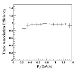
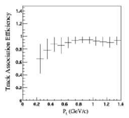
Figure 21: The hit association efficiency between the drift chamber and PC1 (left), and the drift chamber and PC3 (right) as a function of $p_{t}$ in central HIJING 200 GeV/A Au+Au simulated events.

The efficiency of the inter-detector hit association, with the association being defined as the hit closest to the center of the projection window, has been calculated based upon 200 GeV/A Au+Au central events generated using the HIJING event generator [15]. These events were processed through the GEANT-based simulation of the detector response for all detectors in the central arm spectrometers. The output of the response simulation was then reconstructed in the same manner as the data while storing the pointers that relate reconstructed global tracks back to the GEANT tracks that contribute to them. Utilities that trace a reconstructed object back to the GEANT information are implemented as a singleton class for use by a wide variety of evaluations. For the evaluation of the global association, the dominant contributor of the drift chamber track was used as a basis. The dominant contributor is defined as the input GEANT track which contributes the most hits to the reconstructed track. In order for an association to be considered to be made correctly, the GEANT track that provided the reconstructed hit or track for the detector in question must match the dominant contributor of the reconstructed drift chamber track to which it is associated. The efficiency is defined as the ratio of the number of tracks that were correctly reconstructed and geometrically reconstructable to the number of tracks that were geometrically reconstructable by each detector (in order to isolate the efficiency to that of the association only). The results of the efficiency calculation are shown in Fig.  21 for associations to PC1, which is situated adjacent to the drift chamber, and for associations to PC3 after spanning the tracking-detector-free gap occupied by the RICH. Although the efficiencies in the left panel of Fig.  21 are lower, the performance is such that good particle identification can be achieved using the TOF, as demonstrated in the next section.

13 Particle Identification Using the Time-Of-Flight Detector

Particle identification for charged hadrons is performed by combining the information from the drift chamber, PC1, BBC, and the TOF. The time-of-flight resolution of the TOF is measured to be 115 ps, resulting in PID capability for high momentum particles. A 4$\sigma$ $\pi$/K separation at momenta up to 2.4 GeV/c, and a K/proton separation up to 4.0 GeV/c can be achieved as shown in Fig.  22.

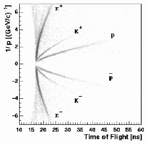
Figure 22: Scatter plot of the time-of-flight versus reciprocal of the momentum in minimum bias Au + Au collisions. This demonstrates the clear particle identification capability using the TOF in the Year 2000 data taking period. The flight path is corrected assuming the mass for each particle species.

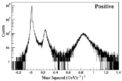
Figure 23: The mass squared distribution for positively charged particles integrated over all momenta.

Once a global track is reconstructed with information from the drift chamber, PC1, and TOF (using a window for TOF association adjusted so that the residuals between the projection point and the reconstructed TOF hit position is within a standard deviation of 2.5), the flight-path length of the track from the event vertex to the TOF as calculated by the momentum reconstruction algorithm is used to correct the time-of-flight value measured by the TOF. Fig.  22 shows a scatter plot of corrected time-of-flight as a function of the reciprocal of the momentum in minimum-bias Au+Au collisions, after the momentum-dependent residual cut between the track projection point and TOF hits. The flight path is also corrected for each particle species in this figure. Fig.  23 shows the mass-squared distribution for positively charged particles integrated over all momenta. The vertical axis in this figure is in arbitrary units. It is demonstrated that clear particle identification using the TOF is achieved in Run 2000.

14 Summary

This document has described the methods and algorithms used for event reconstruction in the PHENIX central arm spectrometers. Using a modular, object-oriented implementation, widely disparate algorithms from widely disparate detector types have been integrated into a coherent reconstruction chain in order to successfully reconstruct hits and tracks within each detector, associate hits from different detectors, reconstruct particle momenta, and provide particle identification for PHENIX physics analysis.

15 Acknowledgements

We thank the staff of the RHIC project, Collider-Accelerator, and Physics Departments at BNL and the staff of PHENIX participating institutions for their vital contributions. We acknowledge support from the Department of Energy and NSF (U.S.A.), Monbu-sho and STA (Japan), RAS, RMAE, and RMS (Russia), BMBF and DAAD (Germany), FRN, NFR, and the Wallenberg Foundation (Sweden), MIST and NSERC (Canada), CNPq and FAPESP (Brazil), IN2P3/CNRS (France), DAE (India), KRF and KOSEF (Korea), and the US-Israel Binational Science Foundation.

References

- [1] The PHENIX Collaboration, Nucl. Phys. A 638 (1998) 565c.
- [2] V. Riabov, Nucl. Inst. Meth. A 419 (1998) 363.
- [3] A. Chikanian, et. al., Nucl. Inst. Meth. A 371 (1996) 480.
- [4] P. Nilsson, et. al., Nucl. Phys. A 661 (1999) 665c.
- [5] L. Carlén, et. al., Nucl. Inst. Meth. A 396 (1997) 310.
- [6] Y. Akiba, et. al., Nucl. Inst. Meth. A 433 (1999) 143.
- [7] Y. Akiba, et. al., Nucl. Inst. Meth. A 453 (2000) 279.
- [8] M. Rosati, et. al., Nucl. Phys. A 661 (1999) 669c.
- [9] T. Peitzmann, et. al., Nucl. Inst. Meth. A 376 (1996) 368.
- [10] G. David, et. al., 1997 IEEE Nuclear Science Symposium Albuquerque, NM, Nov. 9-15, 1997.
- [11] K. Ikematsu, et. al., Nucl. Inst. Meth. A 411 (1998) 238.
- [12] S. N. White, Nucl. Inst. Meth. A 409 (1998) 618.
- [13] C. Adler, A. Denisov, E.Garcia, M.Murray, H.Strobele, and S. White “The RHIC zero degree calorimeters” accepted for publication in NIM A. See nucl-ex/0008005
- [14] M. Bennett, et. al., Nucl. Phys. A 661 (1999) 661c.
- [15] X-N. Wang and M. Gyulassy, Phys. Rev. D 44 (1991) 3501.
- [16] T. Svensson, Ph.D. thesis, Lund University (1999).
- [17] B. Yu, Ph.D. thesis, University of Pittsburgh (1991), BNL 47055 Informal Report.
- [18] E. Gatti et al., Nucl. Instr, and Meth. 163 (1979), 83.
- [19] R. Brun and F. Carminati, CERN Program Library, Long Writeup W5013, March 1994.
- [20] D. Ben-Tzvi and M. B. Sandler, Patt. Rec. Lett. 11 (1990) 167.
- [21] M. Ohlsson, et. al., Comp. Phys. Comm. 71 (1992) 77.
- [22] V. K. Ermilova, et. al., Sov. Phys. JETP 29 (1969) 861.
- [23] F. Sauli, CERN Preprint 77-09 May 1977.
- [24] R. Bellazzini and M. A. Spezziga, INFN PI/AE-94/02.
- [25] A. Lednev, IHEP Preprint 93-153. Protvino, 1993.
- [26] G. David, et. al., IEEE Trans. Nucl. Sci. 43 (1996) 1491.
- [27] G. David, et. al., IEEE Trans. Nucl. Sci. 45 (1998) 705.
- [28] A. Bazilevsky et. al., Instrum. Exp. Tech 41 (1998) 792.
- [29] D. E. Groom, et. al. The European Physical Journal C 15 (2000) 1.