Fragment size correlations in finite systems - application to nuclear multifragmentation

Abstract

We present a new method for the calculation of fragment size correlations in a discrete finite system in which correlations explicitly due to the finite extent of the system are suppressed. To this end, we introduce a combinatorial model, which describes the fragmentation of a finite system as a sequence of independent random emissions of fragments. The sequence is accepted when the sum of the sizes is equal to the total size. The parameters of the model, which may be used to calculate all partition probabilities, are the intrinsic probabilities associated with the fragments. Any fragment size correlation function can be built by calculating the ratio between the partition probabilities in the data sample (resulting from an experiment or from a Monte Carlo simulation) and the ’independent emission’ model partition probabilities. This technique is applied to charge correlations introduced by Moretto and collaborators. It is shown that the percolation and the nuclear statistical multifragmentaion model (smm) are almost independent emission models whereas the nuclear spinodal decomposition model (bob) shows strong correlations corresponding to the break-up of the hot dilute nucleus into nearly equal size fragments.

PACS numbers: 25.70.Pq, 24.60.Ky, 05.10.-a, 24.10.Lx

I Introduction

The break-up of any finite composite system (atomic clusters, atomic nuclei, fullerenes, molecules…) is characterized by a probability distribution which incorporates constraints imposed by dynamical or static conservation laws. Thus, in the case of nuclear decay, the observed multifragmentation modes provide information on properties of nuclear matter at high excitation energy. From a statistical view point the simplest fragmentation model may be formulated by attributing an independent emission probability to each type of fragment (mass, charge). In the limit of infinite parent system size the resulting model (which will be referred to herein as the independent emission model) exhibits no correlation between fragments. For finite systems, we show hereafter that the correlations induced by the static conservation laws, that is in mass and/or charge (referred to hereafter as trivial correlations), can be exactly calculated. In the independent emission model, all the physical information is contained in the emission probabilities of the different types of particles. However, because of the static conservation laws, these intrinsic probabilities are not equal to the observed probabilities.

Most theoretical multifragmentation models, which describe the process of instantaneous break-up of the atomic nucleus submitted to extreme temperature and pressure conditions, introduce other forms of correlations between particle types. When these correlations are specific to a given model, their experimental observation constitutes a crucial test of validation/invalidation. For example, several models, describe the decay of hot nuclei by the development of density fluctuations (surface or volume instabilities [1, 2, 3, 4]). Among these models, the spinodal nuclear decomposition mechanism may dominate when the collision between two nuclei leads to a highly heated and sufficiently compressed nucleonic system. The decompression phase leads the system into the spinodal zone (zone in which the incompressibility modulus $(\partial P/\partial\rho)_{S}$ is negative) where the density fluctuations are exponentially amplified up to produce fragmentation [5]. The dynamics of the density waves in the system is dominated by the most un-stable mode, whose wave length is of the order of 10 fm. Thus the composite nucleus will disintegrate into almost equal size fragments (in the range $Z\approx 6-20$ and, more particularly, $Z\approx 10-15$, see Section IV D).

Binary sequential de-excitation models (gemini[6] or simon [7, 8]) do not exhibit, of course, any preferential decay into equal charges. Nor do instantaneous multifragmentation models : the Copenhagen-Moscow model (code smm) [9] (see Ref. [10] for the system Xe+Sn at 32 $A$ MeV, and the Section IV B of the present article) and the Berlin model [11] (code mmmc) [12].

Experimentally, the charge distributions are privileged tools for the the study of nuclear multifragmentation. However, the yields of various charges alone do not permit a sufficient discrimination of mechanisms. Model validations thus require the comparison of intra-event charge correlations. In this context, a difficulty arises from the fact that the detected fragments are not produced only at the multifragmentation stage of the reaction. Certain light particles, for example, are emitted during the inter-penetration of the nuclear spheres (pre-equilibrium phase), others are emitted, at the end of the process, by the hot multifragmentation fragments. The final (detected) partitions have thus, in part, lost the memory of the crucial moment of the reaction. Therefore, it may be necessary to use statistical methods in order to detect the charge correlations induced by the initial multifragmentation. One of these methods, proposed by L. Moretto and collaborators [13], was shown to be especially efficient for detecting the presence of the spinodal decay mechanism (volume instabilities) of the nucleus.

The fragments formed during the spinodal decomposition phase have comparable sizes (charges). However, this effect is not visible in the charge spectra generated by a Monte-Carlo code (Brownian One Body Dynamics, bob code [5]) simulating this type of mechanism. The reasons are numerous : coalescence and primary fragment deexcitation, finite size effect inducing mode superpositions …The same remark applies to the experimental charge distributions : no excess yield is visible in the expected charge domain. However, the method of charge correlations reveals, for this model, a small ”fossil” signal which corresponds to events in which the system breaks into similar size fragments and whose charges have not been modified (or reduced by the same quantity) before detection. The method introduced by Moretto and collaborators consists in calculating the correlation function of the mean charge $\langle Z\rangle$ of the $M$ imf and of their standard deviation $\sigma$. A peak appears therefore in this correlation function for $\sigma\approx 0$ and $\langle Z\rangle\approx 10-15$. Experimentally, a peak has been effectively observed for the Xe+Sn system at 32 $A$ MeV in central collisions with the indra multidetector [10, 14]. Preferential decompositions in three approximately equal size fragments were also observed in central Xe+Cu reactions at 45 $A$ MeV with the multics multi-detector [15].

The goals of this article are the following :

• We wish to make the interpretation of correlations more rigorous. Progress is necessary because the peak related to spinodal decomposition is often generated by a very small number of experimental or synthesized events. It corresponds, as we will see, to the ratio of two very small quantities and therefore will be characterized by a large error bar. The significance associated with a peak must therefore be systematically evaluated. To this end, we show that the error in the denominator of the correlation function can be greatly reduced by substituting a convolution product for the random selection process proposed in the initial method.

• The correlation peak corresponding to the spinodal decomposition (or to any other cause) is superimposed on a dominant structure due to the correlations induced by the total charge conservation law (trivial correlations). This structure often makes the interpretation of the peaks in terms of physically interesting correlations difficult or ambiguous. Hence, it is important to correct the correlation function for finite size effects. For this reason, it has been proposed to construct the denominator of the correlation function in a different way than that introduced in Ref. [13] using the minimum information model. It will be shown that this method can hide peaks corresponding to non trivial correlations.

• We therefore introduce, in an algebraical exact way, the effects of charge conservation using the independent emission model. Thanks to this new method, any event sample with only trivial correlations will show a flat correlation function.

• We will study more completely the independent emission model constrained by the charge conservation. The notion of intrinsic probability of particles will be introduced.

• Finally, this new method will be validated by its application to three nuclear decomposition models (smm, percolation [16] and bob). It will be shown that these models are, to first order, independent emission models.

II The charge correlation function

A Algebraic calculation of the denominator

The quantity $1+R(\langle Z\rangle,\sigma|M)=P(\langle Z\rangle,\sigma|M)/P_{\rm uc}(\langle Z\rangle,\sigma|M)$, where $\langle Z\rangle$ is the mean charge of the imf, $\sigma$ their standard deviation and $M$ their multiplicity, will be called the charge correlation. The method traditionally used to calculate the denominator of a correlation function [13] consists in constructing ”pseudo-events” using randomly selected fragments belonging to different events of the sample with a given imf multiplicity. The global variable distributions relative to the pseudo-events do not contain intra-event correlations. The numerator $P$ and the denominator $P_{\rm uc}$ of the correlation function are calculated in the same way, the first one from the sample events, the second one from the pseudo-events. Since the denominator does not contain intra-event correlations, its probability density function is written with an index uc (un-correlated).

The only experimental information required for the calculation of the denominator is the charge distribution of the sample. It is equivalent, and, from a computational point of view, faster, to sort charges with respect to the average charge distribution, rather than to select fragments among events. In fact, the random selection using the charge probability distribution is not even necessary since the denominator can be calculated algebraically in the form of a convolution product.

One notes $P(\langle Z\rangle|M)$ the probability to obtain a value $\langle Z\rangle$ of the mean imf charge for the multiplicity $M$ events ($\sum_{\langle Z\rangle}P(\langle Z\rangle|M)=1$, hereafter all conditional probabilities will be assumed to be normalized by a relation of the same type). This conditional probability is given by the convolution :

$$P_{\rm uc}(\langle Z\rangle|M)=\sum_{Z_{1}}\ldots\sum_{Z_{M-1}}P_{Z}(Z_{1}|M)$$ (1)

$$\ldots P_{Z}(Z_{M-1}|M)\ P_{Z}(M\langle Z\rangle-(M-1)\langle Z\rangle^{\prime}\ |M),$$ (2)

where $\langle Z\rangle^{\prime}$ is the mean charge of the imf except the last and $P_{Z}(Z|M)$ the imf charge probability distribution for a given multiplicity. The last factor accounts for the imf total charge conservation ($\sum_{i=1}^{M}Z_{i}=M\ \langle Z\rangle$). The standard deviation is calculated according to the measure :

$$\sigma=\sqrt{\frac{1}{M}\ \sum_{i=1}^{M}(Z_{i}-\langle Z\rangle)^{2}}.$$ (3)

The equations obtained with the un-biased estimator of the standard deviation, used in Ref. [13] are listed in Appendix. The choice of the expression of the standard deviation will not have any influence on the shape of the correlation functions nor on the conclusions of this study. It can be shown that the probability to obtain a standard deviation $\sigma$, when the fragments are randomly selected, is :

$$P_{\rm uc}(\sigma|M)=\sum_{Z_{1}}\ldots\sum_{Z_{M-1}}P_{Z}(Z_{1}|M)\ldots$$ (4)

$$\times P_{Z}(Z_{M-1}|M)\ P_{Z}(\langle Z\rangle^{\prime}+M\ \sqrt{\frac{\sigma^{2}}{M-1}-\frac{\sigma^{\prime 2}}{M}}\ |M)$$ (5)

$$\times P_{Z}(\langle Z\rangle^{\prime}-M\ \sqrt{\frac{\sigma^{2}}{M-1}-\frac{\sigma^{\prime 2}}{M}}\ |M)\,,$$ (6)

where $\sigma^{\prime}$ is the standard deviation of the charges of the imf except the last. If the term under the square root is negative, the probability is zero. Finally the correlation between the mean charge and the standard deviation reads :

$$P_{\rm uc}(\langle Z\rangle,\sigma\ |M)=\sum_{Z_{1}}\ldots\sum_{Z_{M}}P_{Z}(Z_{1}|M)\ldots$$ (7)

$$\times P_{Z}(Z_{M-1}|M)\ P_{Z}(Z_{M}|M)\ \delta_{Z_{M},M\langle Z\rangle+(M-1)\langle Z\rangle^{\prime}}$$ (8)

$$\times\delta_{Z_{M},\langle Z\rangle^{\prime}\pm M\ \sqrt{\frac{\sigma^{2}}{M-1}-\frac{\sigma^{\prime 2}}{M}}}\ ,$$ (9)

where $\delta_{a,b}$, the Kronecker symbol, is equal to 1 when $a=b$ and 0 otherwise. The multinomial decomposition leads to an equivalent (but more practical) form of this equation :

$$P_{\rm uc}(\langle Z\rangle,\sigma\ |M)\ =$$ (10)

$$\ M!\ \sum_{{{{\bf N}\atop\sum_{Z}N_{Z}=M}\atop\sum_{Z}ZN_{Z}=M\langle Z\rangle}\atop\sum_{Z}Z^{2}N_{Z}=M(\langle Z\rangle^{2}+\sigma^{2})}\ \prod_{Z}\frac{P_{Z}(Z|M)^{N_{Z}}}{N_{Z}!}\,,$$ (11)

where $N_{Z}$ is the number of imf with charge $Z$ and ${\bf N}$ an imf partition. The product runs over all possible imf charges. The probabilities in the denominator respect the normalization : $\sum_{\sigma}\sum_{\langle Z\rangle}P_{\rm uc}(\langle Z\rangle,\sigma\ |M)=1$. Hereafter, for notational simplification, the sum sign of Eq. (10) will be written as $\sum_{\{{\bf N}|M,\langle Z\rangle,\sigma\}}$ and the other sum signs will be formed according to the same logic.

The extension of this formula of the denominator to samples containing a variable number of imf is useful when the experimental statistics is reduced. It is expressed straightforwardly as $P_{\rm uc}(\langle Z\rangle,\sigma)=\sum_{M}P_{M}(M)\,P_{\rm uc}(\langle Z\rangle,\sigma\ |M)$ (where $P_{M}$ is the multiplicity probability distribution of the imf), i.e. :

$$P_{\rm uc}(\langle Z\rangle,\sigma)\ =\ \sum_{\{{\bf N}|\langle Z\rangle,\sigma\}}P_{M}(\sum_{Z}N_{Z})\ (\sum_{Z}N_{Z})!\$$ (12)

$$\prod_{Z}\frac{P_{Z}(Z|\sum_{Z^{\prime}}N_{Z^{\prime}})^{N_{Z}}}{N_{Z}!}\,.$$ (13)

B Statistical error bars

Let us recall that the correlation function is defined by :

$$1+R(\langle Z\rangle,\sigma\ |M)=\frac{P(\langle Z\rangle,\sigma\ |M)}{P_{\rm uc}(\langle Z\rangle,\sigma\ |M)}\,.$$ (14)

where the probability in the numerator is the number of sample events including $M$ imf, with mean charge $\langle Z\rangle$ and standard deviation $\sigma$, divided by the number of events with imf multiplicity $M$. To first order, the sampling variance of a proportion applied to Eq. (14) gives the following error :

$$\Delta(1+R(\langle Z\rangle,\sigma\ |M))=\frac{\sqrt{P(\langle Z\rangle,\sigma\ |M)}}{\sqrt{N(M)}\ P_{\rm uc}(\langle Z\rangle,\sigma\ |M)}\,,$$ (15)

where $N(M)$ is the number of events with $M$ imf in the data sample. The use of formula (10) reduces considerably the statistical error. In the case of a Monte-Carlo selection process, it would be, to the same order :

$$\Delta(1+R(\langle Z\rangle,\sigma\ |M))=\frac{\sqrt{P(\langle Z\rangle,\sigma\ |M)}}{\sqrt{N(M)}\ P_{\rm uc}(\langle Z\rangle,\sigma\ |M)}+$$ (16)

$$\frac{P(\langle Z\rangle,\sigma\ |M)}{\sqrt{N_{\rm uc}(M)}\ P_{\rm uc}(\langle Z\rangle,\sigma\ |M)^{3/2}}\,,$$ (17)

where $N_{\rm uc}(M)$ is the number of pseudo-events generated by random selection for the calculation of the denominator. The last term can be very important in the presence of correlation peaks. The calculation of the error is crucial when the standard deviation is zero, on the one hand because it is these events that we are interested in, and, on the other hand, because the number of events of this type is often very small.

In practical cases, the denominator may be evaluated with a very low uncertainty thanks to Eq. (10) since only the - very low - statistical fluctuations on the charge spectrum alter the result. On the other hand the precision of the numerator depends strongly on the number of events in the considered sample. Furthermore, the error on the error bar (Eq. (15)) depends also on the number of events. Therefore it can be inaccurate. It would therefore be interesting to obtain an evaluation of the error bar using only the value of the denominator. This is possible using the so-called null hypothesis, i.e. that the correlation function is equal to unity (absence of correlation). In the frame of this hypothesis the error bar is :

$$\Delta_{1+R=1}(1+R(\langle Z\rangle,\sigma\ |M))=$$ (18)

$$\frac{1}{\sqrt{N(M)\ P_{\rm uc}(\langle Z\rangle,\sigma\ |M)}}\,.$$ (19)

The significance of a positive correlation (of a peak) is defined as being the probability, in the frame of the null hypothesis, that the peak has a height lower than that observed. Therefore, the higher the peak, the higher the significance. An under-estimation of the significance $\cal S$ can be obtained straightforwardly using the Schwarz inequality :

$${\cal S}\leq\frac{N(M)\ P_{\rm uc}(\langle Z\rangle,\sigma\ |M)^{3}}{\left(P(\langle Z\rangle,\sigma\ |M)-P_{\rm uc}(\langle Z\rangle,\sigma\ |M)\right)^{2}}.$$ (20)

Exact calculations of the significance as well as applications to experimental data will be presented in a forthcoming publication [17].

C Case where all imf have the same charge

1 Numerator

Since the spinodal decomposition peak is expected when all imf have the same charge, we now consider the case where $\sigma=0$. For a fixed imf mean charge, there is now only one imf partition : $\forall i,Z_{i}=\langle Z\rangle$. Thus, differences between the complete partitions with same $\langle Z\rangle$ are only due to the light fragments whose total charge is $z_{\rm light}=z_{\rm tot}-M\langle Z\rangle$.

2 Denominator

When $\sigma=0$, the probabilities given by Eq. (10) become :

$$P_{\rm uc}(\langle Z\rangle,0\ |M)\ \left\{\begin{array}[]{l}=P_{Z}(\langle Z\rangle\ |M)^{M}\cr\hbox{if }\langle Z\rangle\hbox{ is integer and }\cr\langle Z\rangle\in[Z_{\rm min},z_{\rm tot}-(M-1)\ Z_{\rm min}],\cr=0\cr\hbox{otherwise}\,,\end{array}\right.$$ (21)

where $P_{Z}(Z|M)$ is the charge distribution for a given imf multiplicity ($\sum_{Z=Z_{\rm min}}^{z_{\rm tot}}P(Z|M)=1$). The mean charge being equal to the charge of each imf implies that $\langle Z\rangle$ is always an integer. The probability that the standard deviation is zero is :

$$P_{\rm uc}(\sigma=0)\ =\sum_{\langle Z\rangle=Z_{\rm min}}^{z_{\rm tot}-(M-1)Z_{\rm min}}P_{Z}(\langle Z\rangle|M)^{M}\,.$$ (22)

When the charge distribution of light imf follows a power law or an exponential law (we will see that this is the case for the minimum information model), the denominator assumes very simple forms (respectively) :

$$P_{\rm uc}(\langle Z\rangle,0\ |M)\ \propto\langle Z\rangle^{-\tau M}\,,$$ (23)

$$P_{\rm uc}(\langle Z\rangle,0\ |M)\ \propto{\rm e}^{-\tau M\langle Z\rangle}\,.$$ (24)

3 Correlation function

As indicated previously, the evaluation of the correlation function in the case of equal size imf, is of considerable physical interest. Unfortunately it often corresponds to the ratio of two very small probabilities. If the number of events in the sample is too low, it is possible that no event corresponds to the given mean charge (the correlation function cannot be calculated) or that a very small number of events correspond (which can lead to a spurious peak). It is therefore important to determine, a priori, the minimum number of events necessary to obtain a reliable evaluation of the correlation function for a null standard deviation. An evaluation of this number can be obtained making, once more, the hypothesis that the correlation function is unity. The probability to obtain an event in which the imf charges are all equal to $\langle Z\rangle$ is $P_{Z}(\langle Z\rangle|M)^{M}$ (this quantity can be obtained precisely even with a reduced event sample). The minimum size $N(M)$ of the sample must be therefore of one order of magnitude greater than $P_{Z}(\langle Z\rangle|M)^{-M}$.

III Denominator conditioned by charge conservation.

The formation of the denominator as proposed by Moretto and collaborators (that we will continue to call the pseudo-event method though the result is expressed by the algebraic formula (10)) has many advantages : it is rigorous, it is simple to evaluate, it takes into account the efficiency of the detector, it uses only experimentally measured quantities and the resulting correlation function shows all charge correlations, whatever their origin. This latter advantage can become an inconvenience when one wishes to study correlations induced by only one physical cause. In the majority of cases, the main structure in the correlation function is due to the total charge conservation law. We will see that this law introduces a large structure, greater than unity, close to $\langle Z\rangle=z_{\rm tot}/M$. In Ref. [10], this structure was considered as a baseline on which was superimposed a peak due to the spinodal decomposition mechanism.

In this section we will discuss two different propositions for calculating the denominator taking into account the charge conservation (in order to remove the corresponding structure from the correlation function). The first one consists in using partitions provided by the minimum information model (all the partitions of a given total charge have the same probability). We will show that the denominator constructed in this way presents a spurious peak at $\sigma=0$ that can conceal a possible physical peak in the correlation function (Section III A). The second proposition consists in modifying the expression (10) of the algebraic calculation of the denominator in order to introduce, in an exact way, the influence of charge conservation with the consequence that charge conservation influences both numerator end denominator.

A Minimum information model

1 Introduction

In this model, all partitions have the same probability : $P({\bf n})=1/N(z_{\rm tot})$ where $N(z_{\rm tot})$ is the total number of partitions for total charge $z_{\rm tot}$. This result is obtained by application of the minimum information principle (or maximal entropy), information being defined as :

$$I=\sum_{{\bf n}}P({\bf n})\ln{P({\bf n})}.$$ (25)

Setting the derivative of $I$ equal to zero, under the single constraint of charge conservation, one obtains that all probabilities are equal. The total number of charge partitions of a charge $z_{\rm tot}$ nucleus is approximately given by the Ramanujan-Hardy formula [18] whose leading term is :

$$N(z_{\rm tot})\approx\frac{\exp{\left(\pi\sqrt{\frac{2z_{\rm tot}}{3}}\right)}}{4z_{\rm tot}\sqrt{3}}\,.$$ (26)

The number of partitions increases therefore very rapidly with the charge. Thus, studies of large systems, by systematic generation of all partitions, are not possible. The calculation of the number of imf partitions (all fragments have a charge greater than a certain limit) and of light fragments (fragments with charge lower than a certain limit) is exposed in the companion article [19]. Some examples of applications of the minimum information model (possibly modified by combinatorial factors) to nuclear fragmentation are given in Refs. [20, 21, 22, 23, 24]

2 Case where all imf have the same charge

In this subsection, the correlation function for the minimum information model in the case $\sigma=0$ will be calculated exactly. It will be shown that this function presents a combinatorial peak due to an intrinsic feature of the model, namely the non-ordering of the charges. We will introduce an alternative model in which this effect is corrected.

a Numerator.

The numerator $P(\langle Z\rangle,0\ |M)$ of the correlation function is calculated as the number of partitions with $M$ imf, each of charge $\langle Z\rangle$, divided by the total number of partitions with $M$ imf. The charges of the imf being fixed, the number of partitions will be equal to the number of ways to divide the remaining charge $z_{\rm light}=z_{\rm tot}-M\langle Z\rangle$ into light fragments (i.e. fragments with charge less than or equal to $z_{\rm max}=Z_{\rm min}-1$). This constrained number of partitions will be noted ${}^{z_{\rm max}}N(z_{\rm light})$. Similarly, the number of partitions of charge $z$ into $M$ fragments with charge greater or equal to $Z_{\rm min}$ will be noted ${}_{Z_{\rm min}}N(z,M)$. These numbers can be calculated exactly [19]. With our notation, the numerator reads :

$$P(\langle Z\rangle,0\ |M)=$$ (27)

$$\frac{{}^{z_{\rm max}}N(z_{\rm light})}{{\sum_{\langle Z\rangle^{\prime}}}\ {{}_{Z_{\rm min}}N(M\langle Z\rangle^{\prime},M)}\ ^{z_{\rm max}}N(z_{\rm tot}-M\langle Z\rangle^{\prime})}\,.$$ (28)

b Denominator.

We have seen (Eq. (21)) that the denominator is written as $P_{Z}(\langle Z\rangle\ |M)^{M}$ when the standard deviation is zero. The conditional probability of $\langle Z\rangle$ given $M$ is the number of partitions with $M$ imf weighted by the proportion of charges $\langle Z\rangle$ that they contain, divided by the number of partitions containing $M$ imf, so that :

$$P_{\rm uc}(\langle Z\rangle,0\ |M)=$$ (29)

$$\left(\frac{\sum_{\langle Z\rangle=Z_{\rm min}}^{z_{\rm tot}/M}\sum_{\{{\bf N}|\langle Z\rangle,M\}}\frac{N_{\langle Z\rangle}}{M}\ ^{z_{\rm max}}N(z_{\rm tot}-M\langle Z\rangle)}{\sum_{\langle Z\rangle^{\prime}=Z_{\rm min}}^{z_{\rm tot}/M}\ {{}_{Z_{\rm min}}N(M\langle Z\rangle^{\prime},M)}\ ^{z_{\rm max}}N(z_{\rm tot}-M\langle Z\rangle^{\prime})}\right)^{M}$$ (30)

in which the sum over all partitions containing $M$ imf has been written :

$$\sum_{\langle Z\rangle=Z_{\rm min}}^{z_{\rm tot}/M}\sum_{\{{\bf N}|\langle Z\rangle,M\}}\equiv\sum_{Z_{1}}\ldots\sum_{Z_{k}=Z_{k-1}}^{R_{k}/(M-k+1)}\ldots\sum_{Z_{M}}\,,$$ (31)

with $Z_{0}=Z_{\rm min}$ and $R_{k}=z_{\rm tot}-\sum_{i=1}^{k-1}Z_{i}$. The charges of the imf are noted $Z_{i}$ and are written in increasing order.

c Correlation function.

The charge correlation function is thus given by :

$$1+R(\langle Z\rangle,0\ |M)=^{z_{\rm max}}N(z_{\rm tot}-M\langle Z\rangle)$$ (32)

$$\times\left({\sum_{\langle Z\rangle^{\prime}}}\ {{}_{Z_{\rm min}}N(M\langle Z\rangle^{\prime},M)}\ ^{z_{\rm max}}N(z_{\rm tot}-M\langle Z\rangle^{\prime})\right)^{M-1}$$ (33)

$$/\left(\frac{1}{M}\sum_{\langle Z\rangle=Z_{\rm min}}^{z_{\rm tot}/M}\sum_{\{{\bf N}|\langle Z\rangle,M\}}N_{\langle Z\rangle}\ ^{z_{\rm max}}N(z_{\rm tot}-M\langle Z\rangle)\right)^{M}$$ (34)

The latter result is, of course, free of error since it results from the numbering of all possible partitions. Results for two total charges, two multiplicities and two definitions of the imf are presented in Fig. 1.

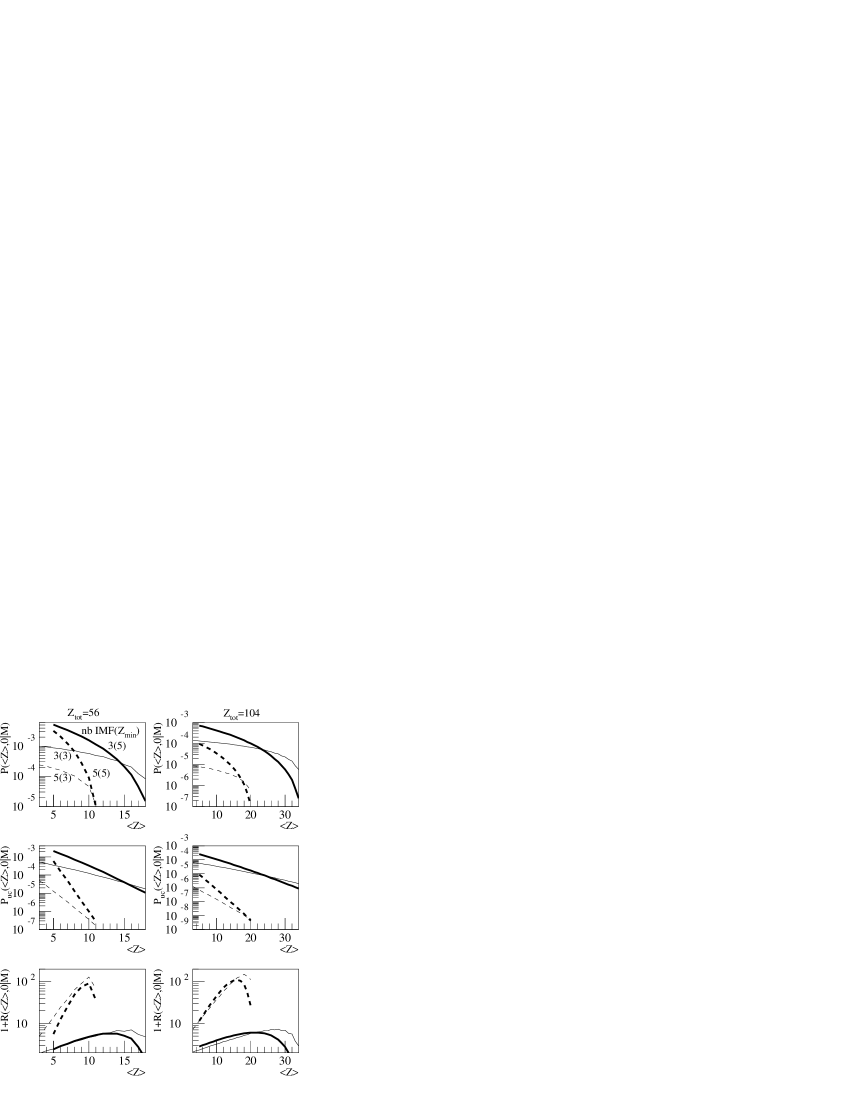
FIG. 1.: Numerator (upper row), denominator (median row) and correlation function (lower row) for total charges 56 (left column) and 104 (right column). The bold lines correspond to imf with minimum charge 5, the thin lines to imf with minimum charge 3. The dotted lines correspond to the events with 5 imf and the full lines to those with 3 imf.

We observe that :

• The behavior of the correlation function depends only weakly on the size of the system. This result has been observed experimentally : similar correlation functions have been observed for very different systems in central collisions [10, 25].

• The denominators are exponentially decreasing. This is due to the fact that the charge distributions are also exponentially decreasing between $Z_{\rm min}$ and $z_{\rm tot}-(M-1)Z_{\rm min}$ (Eq. (23)).

• The abscissa of the maximum of the correlation function is a few units lower than $z_{\rm tot}/M$, this property can be used to provide an experimental determination of the total charge of the composite nucleus, after pre-equilibrium emission, measuring only the imf.

• The amplitude of the correlation function increases strongly as the minimum charge of the imf diminishes and their multiplicity increases.

Fig. 2 presents the correlation function obtained for different multiplicity 3 systems (left column) and for the total charge 79 and different multiplicities (right column).

FIG. 2.: Charge correlation function, for a null standard deviation, obtained by formula (32) in the framework of the minimum information model. Heavy traces correspond to imf with charges greater than 5 and light traces to imf with charges greater than 3. The correlation functions for an imf multiplicity of 3 are presented on the left hand column in which the total charges of systems are, from top to bottom, 79, 104 and 400. The three graphs on the right hand column correspond to the total charge 79 and the imf multiplicity runs from 4 (top) to 6 (bottom). The horizontal lines are placed at $1+R=M!$.

The left hand column shows that the correlation functions are homothetic for a given multiplicity. On each figure a horizontal line has been placed at $1+R(\langle Z\rangle,0|M)=M!$. One oberves that the maximum of the correlation function is always of the order of $M!$. This property is due to the multinomial factors of the denominator (Eq. (10)). When the standard deviation is null, the product $\prod_{Z}N_{Z}!$ is identically equal to $M!$, it factorises therefore in the numerator of the correlation function. When the standard deviation increases, this product decreases rapidly down to 1 when all charges are different. To illustrate this point, let us consider two very similar partitions of the total charge 21 into 3 imf : {7,7,7} and {6,7,8}. The numerator of the correlation function for both partitions is the same : $1/N(21,3)\ (=1/249)$. The denominator is, in the former case, $P(7|3)^{3}\ (=6.6\ 10^{-4})$ and, in the latter case, $3!\ P(6|3)P(7|3)P(8|3)\ (=3!\ 6.04\ 10^{-4})$. Therefore the probability product is almost the same in both cases. Besides, the charge conservation constraint is weak when the imf have small charges hence $1+R(\{6,7,8\})\approx 1$ (one finds 1.1). Consequently $1+R(\{7,7,7\})\approx 3!$ (one finds 6.1).

It can be conjectured that this effect would occur for all non-ordered fragment models. If one multiplies every partition by a factor equal to the number of charge permutations ($M!/\prod_{Z}N_{Z}!$), the peak disappears. On the other hand probabilities for other sigma values are little modified because the $N_{Z}$ are then almost always equal to 0 or 1 (i.e. $\prod_{Z}N_{Z}!=1$). This latter model will be referred to as the ordered minimum information model.

B Algebraic calculation of the denominator with charge conservation

1 Method

The goal of this subsection is to introduce the exact method for the evaluation of the denominator that eliminates the effects due to charge conservation from the correlation function. This denominator is obtained by an extension of the formula (10) to the whole charge (i.e. including light fragments). In a first step, we suppose that there is no correlation at all between charges. This means that each charge is described by a probability ${{}^{\rm intr}P}_{z}(z)$ (that will be referred to as intrinsic probability of the charge). The conditional probability of a partition ${\bf n}$ (including the imf and the light particles) with total multiplicity $m$ is given then by the multinomial formula :

$$P({\bf n}|m)=m!\ \prod_{z}\frac{{{}^{\rm intr}P}_{z}(z)^{n_{z}}}{n_{z}!}\,.$$ (35)

These conditional probabilities obey the normalization condition $\sum_{{\bf n}}P({\bf n}|m)=1$. If one introduces the constraint of total charge conservation, partition constrained conditional probabilities are given by (an index cc will be applied to probabilities constrained solely by the charge conservation) :

$$P_{\rm cc}({\bf n}|m)=k(m)\ m!\ \prod_{z}\frac{{{}^{\rm intr}P}_{z}(z)^{n_{z}}}{n_{z}!}\ \delta_{z_{\rm tot},\sum_{z}z\,n_{z}}\ ,$$ (36)

with :

$$k^{-1}(m)=m!\sum_{\{{\bf n}|m,z_{\rm tot}\}}\prod_{z}\frac{{{}^{\rm intr}P}_{z}(z)^{n_{z}}}{n_{z}!}\,.$$ (37)

On the other hand, the multiplicity probability distribution is given by :

$$P_{m}(m)=\alpha\ m!\,\sum_{\{{\bf n}|m,z_{\rm tot}\}}\prod_{z}\frac{{{}^{\rm intr}P}_{z}(z)^{n_{z}}}{n_{z}!}\,,$$ (38)

with :

$$\alpha^{-1}=\sum_{\{{\bf n}|z_{\rm tot}\}}(\sum_{z}n_{z})!\,\prod_{z}\frac{{{}^{\rm intr}P}_{z}(z)^{n_{z}}}{n_{z}!}\,.$$ (39)

Finally, the partition probabilities are given by :

$$P_{\rm cc}({\bf n})=\alpha\ (\sum_{z}n_{z})!\,\prod_{z}\frac{{{}^{\rm intr}P}_{z}(z)^{n_{z}}}{n_{z}!}\ \delta_{z_{\rm tot},\sum_{z}z\,n_{z}}\ .$$ (40)

These probabilities contain all the information relative to the charges and to their correlations. For example, (observed) charge and conditional charge probability distributions are given respectively by :

$$\begin{array}[]{ll}P_{z}(z_{0})&=\frac{\sum_{{\bf n}}n_{z_{0}}\,P_{\rm cc}({\bf n})}{\sum_{{\bf n}}(\sum_{z}n_{z})\,P_{\rm cc}({\bf n})}\\ &=\frac{\alpha}{\langle m\rangle}\ \sum_{\{{\bf n}|z_{\rm tot}\}}n_{z_{0}}\,(\sum_{z}n_{z})!\,\prod_{z}\frac{{{}^{\rm intr}P}_{z}(z)^{n_{z}}}{n_{z}!}\,,\\ P_{z}(z_{0}|m)&=\frac{1}{P_{m}(m)}\sum_{\{{\bf n}|m\}}\frac{n_{z_{0}}}{m}\ P_{\rm cc}({\bf n})\\ &=\frac{\sum_{\{{\bf n}|m,z_{\rm tot}\}}n_{z_{0}}\,\prod_{z}\frac{{{}^{\rm intr}P}_{z}(z)^{n_{z}}}{n_{z}!}}{m\,\sum_{\{{\bf n}|m,z_{\rm tot}\}}\prod_{z}\frac{{{}^{\rm intr}P}_{z}(z^{n_{z}})}{n_{z}!}}\,.\end{array}$$ (41)

Because of correlations, the intrinsic probabilities are not equal to the probabilities to observe the charges (the conservation constraint favours small charges, see Fig. 3b). Equality between intrinsic probabilities and observed probabilities is valid only for an infinite system.

The intrinsic probabilities are quantities which are not directly measurable, they must be calculated by inversion of Eq. (40) where the $P_{\rm cc}({\bf n})$ are the measured frequencies of the partitions. The set of Eqs. (41) constitutes an under-determined system. It is thus not possible to obtain an unique solution.

However, inversion of (40) is possible if the non trivial correlations between charges in the studied sample are weak. When the intrinsic probabilities are determined, the probabilities of the denominator can be calculated by summing the complete partition probabilities having the same imf mean charge and standard deviation :

$$P_{\rm cc}(\langle Z\rangle,\sigma|M)=\frac{1}{P_{M}(M)}\sum_{\{{\bf n}|M,\langle Z\rangle,\sigma\}}P_{\rm cc}({\bf n})\,.$$ (42)

Finally we can write that the denominator is constructed using the intrinsic probabilities :

$$P_{\rm cc}(\langle Z\rangle,\sigma|M)=$$ (43)

$$\frac{\sum_{\{{\bf n}|z_{\rm tot},M,\langle Z\rangle,\sigma\}}\,(\sum_{z}n_{z})!\,\prod_{z}\frac{{{}^{\rm intr}P}_{z}(z)^{n_{z}}}{n_{z}!}}{\sum_{\{{\bf n}|z_{\rm tot},M\}}\,(\sum_{z}n_{z})!\,\prod_{z}\frac{{{}^{\rm intr}P}_{z}(z)^{n_{z}}}{n_{z}!}}\,.$$ (44)

This new denominator takes explicitly into account the charge conservation. Structures observed in the corresponding correlation function will necessarily arose from other causes.

2 Monte-Carlo generation of events without non trivial charge correlations

A sample of events without non trivial correlations may be synthesized by the following procedure. Charges $z_{i}$ are selected randomly according to their intrinsic probabilities until $\sum_{i}z_{i}\geq z_{\rm tot}$. The event is preserved only if $\sum_{i}z_{i}=z_{\rm tot}$. The resulting charge spectra are those given by Eqs. (41). The alternative procedure that would consist in randomly selecting $M-1$ charges, and deducing the last charge using charge conservation would introduce a bias since the distribution of the last charge would be different from the preceding ones.

3 Combinatorial independent emission models

We stated previously that models can be characterized by the term ”independent emission” if they contain no correlations, other than those induced by the conservation of the total charge. This definition implies that partition probabilities generated by such models can be written in the form of Eq. (40). We give here two examples of independent emission models.

a Ordered minimum information model.

The model produced by weighting partitions by a factor $m!/\prod_{z}n_{z}!$ is an independent emission model. One notes that this weighting is the same as the one of Eq. (40) if the product $\prod_{z}{{{}^{\rm intr}P}_{z}}(z)^{n_{z}}$ is constant. This condition is fulfilled if and only if ${{}^{\rm intr}P}_{z}(z)=a^{z}$ (the intrinsic probability product is $a^{z_{\rm tot}}$). Thus, the normalization of the probabilities is $\sum_{z}a^{z}=1$. For a sufficiently large total charge (in practice, superior to 10), the normalization condition implies $a=1/2$. The model in which every partition is weighted by the number of permutations of its charges ($m!/\prod_{z}n_{z}!$) is therefore an independent emission model with intrinsic probabilities ${{}^{\rm intr}P}_{z}(z)=2^{-z}$. The resulting charge distributions are almost exponentially decreasing (Fig. 3a). Conversely, the minimum information model is not an independent emission model (it is not possible to find a set of intrinsic probabilities such that all partition probabilities would be the same).

b Model of charge equi-probability.

The minimum information model is taken as implying the equi-probability of the partitions. In this context it is also interesting to see results given by another elementary model obtained by assuming intrinsic equi-probability of the charges. The resulting charge distribution is of course not uniform because of the constraint of conservation of the total charge.

The Eq. (40), for ${{}^{\rm intr}P}_{z}(z)=1/z_{\rm tot}$, gives :

$$\begin{array}[]{lll}P_{\rm cc}({\bf n})&=&\alpha\,(\sum_{z}n_{z})!\,\prod_{z}\frac{\left(\frac{1}{z_{\rm tot}}\right)^{n_{z}}}{n_{z}!}\ \delta_{z_{\rm tot},\sum_{z}z\,n_{z}}\\ &=&\frac{\alpha\,m!}{z_{\rm tot}^{m}\,\prod_{z}n_{z}!}\ \delta_{z_{\rm tot},\sum_{z}z\,n_{z}}\ ,\end{array}$$ (45)

In other words, if one generates partitions by imposing charge conservation and if all charges have the same intrinsic probability to be selectioned, then the partition weight is $m!/(z_{\rm tot}^{m}\,\prod_{z}n_{z}!)$. Examples of observed charge spectra are given for different values of the total charge in Fig. 3b). These spectra are very different from that of the intrinsic probabilities. Indeed one observes an almost exponential decrease. Only the last charge has a probability which is not consistent with this tendency. This behaviour is due to the fact that the charge $z_{\rm tot}-1$ can appear accompanied only by a charge 1, whereas the charge $z_{\rm tot}$ is never rejected. More precisely, Eq. (41) gives $P_{z}(z_{\rm tot})=(z_{\rm tot}/2)\ P_{z}(z_{\rm tot}-1)$. One notices that the greater the total charge the less the influence of the constraint of conservation and consequently the smaller the slope of the exponential.

FIG. 3.: Charge distributions obtained in the ordered minimum information model (a) and in the charge equi-probability model (b) constrained by total charge conservation. Circles correspond to a total charge of 20, squares to $z_{\rm tot}=56$ and points to $z_{\rm tot}=104$. The full lines are the intrinsic probability distributions.

4 Multiplicity constrained independent emission model

We now consider the model for which probabilities of partitions with fixed multiplicity are given by Eq. (35), but the multiplicity probability distribution is not given by the combinatorial Eq. (38). The multiplicity probability distribution $P_{m}(m)$ is imposed a priori. This model has been studied extensively by A.J. Cole and collaborators [24]. The main difference between the quoted articles and the study presented in this paragraph resides in the interpretation of quantities noted $X_{z}$ by Cole et al. and, here, ${{}^{\rm intr}P}_{z}$ as, respectively, adjustable parameters and intrinsic probabilities. However, the $X_{z}$ parameters being defined to a factor $a^{z}$, it is always possible to normalize them. Indeed, the product $\prod_{z}(a^{z}X_{z})^{n_{z}}$ is equal to the product $\prod_{z}X_{z}^{n_{z}}$ to within a constant ($a^{z_{\rm tot}}$). Eq. (35) and the normalizations give :

$$P_{\rm cc}({\bf n})=\frac{P_{m}(m)}{\sum_{\{{\bf n}^{\prime}|m,z_{\rm tot}\}}\prod_{z}\frac{{{}^{\rm intr}P}_{z}(z)^{n^{\prime}_{z}}}{n^{\prime}_{z}!}}$$ (46)

$$\times\prod_{z}\frac{{{}^{\rm intr}P}_{z}(z)^{n_{z}}}{n_{z}!}\ \delta_{z_{\rm tot},\sum_{z}z\,n_{z}}\ ,$$ (47)

with :

$$m=\sum_{z}n_{z}\,.$$ (48)

In the same way as for charges, one can introduce an intrinsic probability for multiplicities (${{}^{\rm intr}P}_{m}$). The partition probability is then written as :

$$P_{\rm cc}({\bf n})=k\ {{}^{\rm intr}P}_{m}(m)\ m!\ \prod_{z}\frac{{{}^{\rm intr}P}_{z}(z)^{n_{z}}}{n_{z}!}\ \delta_{z_{\rm tot},\sum_{z}z\,n_{z}}\ ,$$ (49)

with :

$$k^{-1}=\sum_{m}\ {{}^{\rm intr}P}_{m}(m)\ m!\sum_{\{{\bf n}|m,z_{\rm tot}\}}\prod_{z}\frac{{{}^{\rm intr}P}_{z}(z)^{n_{z}}}{n_{z}!}\,.$$ (50)

One deduces the relation between observed probabilities of multiplicities and those of the intrinsic probabilities :

$$P_{m}(m)=\ {{}^{\rm intr}P}_{m}(m)$$ (51)

$$\left[\frac{m!\ \sum_{\{{\bf n}|m,z_{\rm tot}\}}\ \prod_{z}\frac{{{}^{\rm intr}P}_{z}(z)^{n_{z}}}{n_{z}!}}{\sum_{m^{\prime}}\ {{}^{\rm intr}P}_{m}(m^{\prime})\ m^{\prime}!\ \sum_{\{{\bf n}|m^{\prime},z_{\rm tot}\}}\prod_{z}\frac{{{}^{\rm intr}P}_{z}(z)^{n_{z}}}{n_{z}!}}\right]$$ (52)

Intrinsic probabilities and observed probabilities possess the same distributions in the limit of an infinite system size.

IV Applications

A Introduction

In this section we show the charge correlation obtained, for several nuclear decay models, using the denominator given by the independent emission hypothesis. The first step of the procedure consists in determining the intrinsic probabilities of the charges for each model sample. These probabilities are obtained by a recursive procedure of minimization of the $\chi^{2}$ between probabilities of partitions in the synthesized sample and those given by Eq. (36). The convergence of the procedure is possible only if non trivial correlations between charges are weak. The minimum $\chi^{2}$ is therefore an indication of the strength of these correlations. The second step, calculation of the denominator by the method presented in Section III B 1 (43), would also not be possible in the presence of strong correlations. We will see that this condition is fulfilled by the three models that we are going to study. Results of the application of this procedure to the experimental events will be presented in forthcoming articles [17, 25].

B The Copenhagen model

The Copenhagen model [9, 26] is a hot liquid drop model that describes the multifragmentation of the nucleus as an instantaneous statistical mechanism. The probability of a partition in mass and in charge $n_{a,z}$ for an excitation energy $E^{*}$ is given by :

$$P({\bf n}|E^{*})=P_{I}(E^{*})\ \left[\frac{V_{F}}{\lambda_{T}^{3}}\right]^{m}\left[\prod_{a,z}\frac{a^{3n_{a,z}/2}}{n_{a,z}!}\right]$$ (53)

$$\times\delta_{a_{\rm tot},\sum_{a,z}a\ n_{a,z}}\ \delta_{z_{\rm tot},\sum_{a,z}z\ n_{a,z}}\ .$$ (54)

The two Kronecker symbols account for the conservation of mass and of charge. The de Broglie wavelength of the nucleon $\lambda_{T}=\sqrt{2\pi\hbar/(m_{n}T)}$ depends on the temperature which is roughly constant at fixed excitation energy. The density of states corresponding to the internal excitation energy of the fragments $P_{I}(E^{*})$ is also constant at a given excitation energy. In this model, as in comparable models, the multiplicity is correlated linearly with the excitation energy, a prediction which is verified by experimental observation. The first two factors can be considered therefore to be constant for a given multiplicity. The volume of the nucleus at the time of fragmentation, $V_{F}$, is supposed to be independent of the partition (or, according to the version of the model, dependent only on the multiplicity). If we disregard the conservation of the mass, the emission probability of a fragment is proportional to $a^{3/2}$ : $P_{z}(z)=\alpha\,a^{3/2}$, so that the product $\prod_{z}P_{z}(z)^{n_{z}}=\alpha^{m}\prod_{z}a^{3n_{z}/2}$ involves a new factor depending only on the multiplicity. The equation can therefore be re-written as :

$$P({\bf n}|m)\propto\prod_{z}\frac{P_{z}(z)^{n_{z}}}{n_{z}!}\ \delta_{z_{z_{\rm tot}},\sum_{z}z\ n_{z}}\ ,$$ (55)

so that we recover the same expression as that obtained for the independent emission model. We thus expect that the correlation function is everywhere equal to 1 and if the denominator is calculated from pseudo-events, we expect that the shape of the correlation function is determined by charge conservation. However, this conclusion is based on a simplified form of the model. The correlation function may thus exhibit weak modulations. Moreover, one does not expect a peak for small values of the standard deviation.

Using the smm code, 35 million events have been generated for the ¹³⁸Ba nucleus excited to 5 MeV per nucleon. We built, from this sample, the charge correlation function for the imf. The Copenhagen model produces results (almost) consistent with independent emission as shown in Fig. 4. Discrepancies can be explained notably by the fact that the hot fragments produced during the multifragmentation phase described by Eq. (53), thereafter decay by light particle emission.

FIG. 4.: Comparison of charge spectra for several multiplicities for smm (circles) and for the independent emission hypothesis (lines). The dashed line corresponds to the intrinsic probabilities. The multiplicity probability distributions, $P_{m}(m)$, given by the two models are also shown in the figure.

The charge correlation functions calculated with the denominators of formulas (10) and (43) are presented in the Figs. 5 and 6. In the first case, the main structures are due to the conservation of the charge, in the second, the correlation function is practically flat. Non trivial correlations between charges are therefore very weak for this model and no preferential fragmentation into equal charge is observed. The - small - modulations of the correlation function are due to physical causes and to statistical fluctuations.

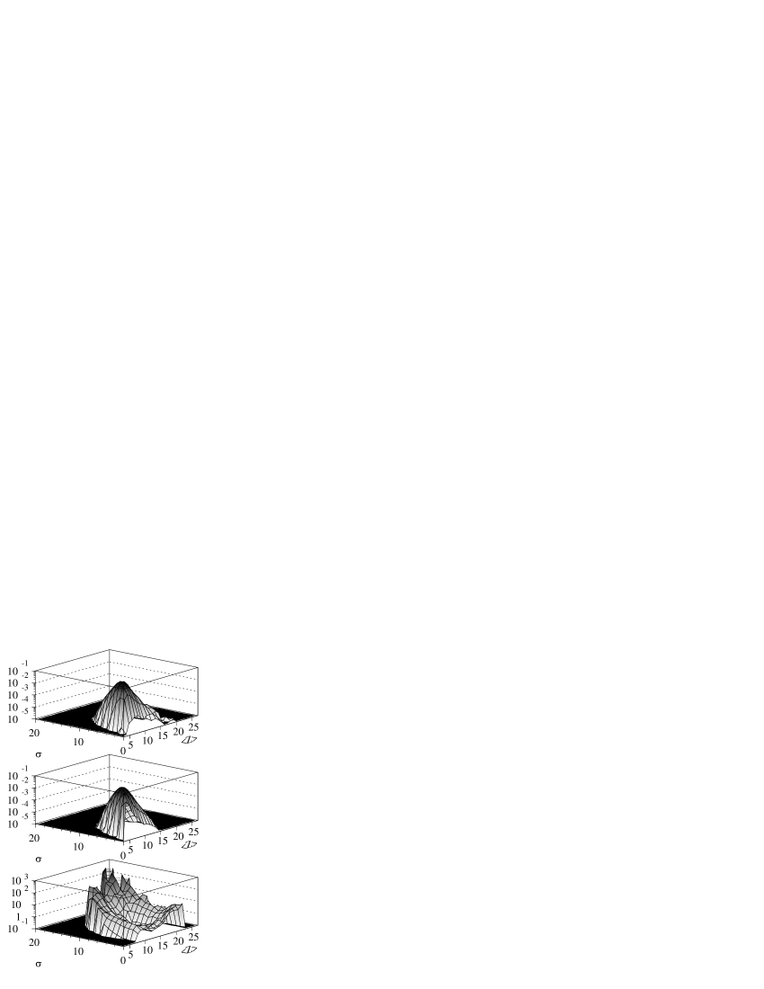
FIG. 5.: Upper and lower figures present, in order, the numerator, denominator and $[\langle Z\rangle,\sigma]$ correlation function for the Copenhagen model. The denominator is calculated by the method of pseudo-events (formula (10)).

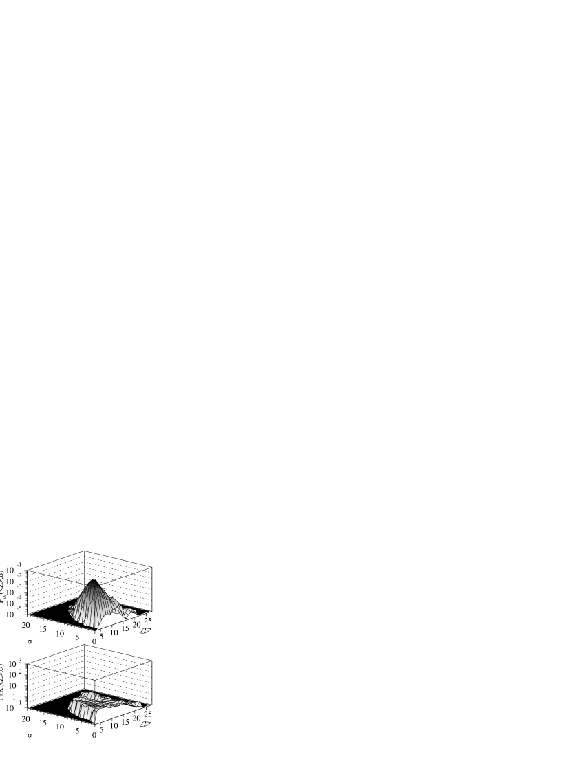
FIG. 6.: Denominator (upper figure) and correlation function (lower figure) of $[\langle Z\rangle,\sigma]$ for the Copenhagen model (the numerator is presented at the top of the previous figure). The denominator is calculated using the independent emission hypothesis, via formula (43).

C Percolation

The same study has been carried out on a sample obtained with a percolation code [16]. A sample of 10⁸ events has been generated using a 3D percolation program on a simple cubic 4$\times$4$\times$4 periodic frame, for a bond breaking probability of 70 %. The result of the $\chi^{2}$ minimization process is presented Fig. 7 in which are compared charge distributions for various multiplicities in percolation and those given by the formula (36) (the intrinsic probabilities are indicated by a dotted line). The very good agreement indicates that the correlations between charges are very weak in this model.

FIG. 7.: Percolation (same conventions as in Fig. 4.)

Figs. 8 and 9 present percolation correlation functions obtained using denominators given respectively by the pseudo-event method (Eq. (10)) and by the independent emission hypothesis (Eq. (43)). These figures were constructed for all possible values of the number of imf. In the first case, structures are almost entirely due to the conservation of the charge (to each imf multiplicity corresponds an edge line). When the denominator is calculated using the intrinsic probabilities, the correlation function is flat and equal to 1 (Fig. 9). The small peaks on the sides of the correlation function are due to the statistical fluctuations.

The model of percolation can therefore be assimilated to knowledge of the intrinsic probabilities.

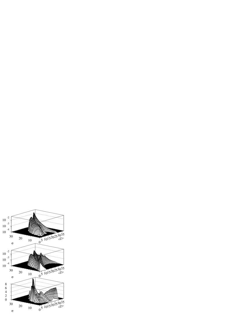
FIG. 8.: Percolation (same conventions as in Fig. 5.)

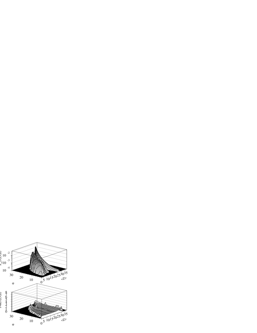
FIG. 9.: Percolation (same conventions as in Fig. 6.)

Fig. 10 presents the correlation function of the percolation calculation when the denominator is calculated with the minimum information model (upper figure) and with the ordered minimum information model (lower figure) for same total charge ($z_{\rm tot}=64$). In both cases, the correlation function presents large structures which are not easily interpreted.

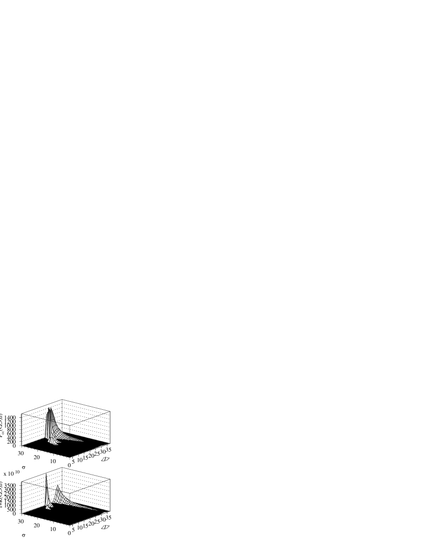
FIG. 10.: Correlation function of $[\langle Z\rangle,\sigma]$ for the percolation process (the numerator is presented at the top of Fig. 8). Denominators are given by the models of the minimum information (upper figure) and of the ordered minimum information (lower figure).

D The Brownian One Body dynamical model

The last model to be studied in this work is characterized by non trivial correlations, even though, as motioned in the introduction, they are partly masked by different processes. The preferential decomposition of the system into almost equal charges (in the range $[10,20]$), which characterizes the bob model, is not visible, for example, in the inclusive charge spectra (Fig. 11).

Our simulated sample was obtained via a four step process [27]. The collision entrance channel has been simulated using a one-body semi-classical microscopic calculation of the bnv type [28] for the system ¹²⁹Xe + ¹¹⁹Sn at 32 $A$ MeV. This calculation shows that, for the most central collisions, a compressed single source is formed, after a weak pre-equilibrium emission, within 40 fm/c. The decompression phase, the entrance into the spinodal zone and the formation of the fragments are then followed by the bob code which simulates Boltzmann-Langevin density fluctuations [29] and the evolution of the system density submitted to spinodal instabilities. In a third step, fragments are formed using an algorithm which regroups contiguous cells which numbers of test particles (40 test particles are used to simulate a nucleon) is greater than a given threshold. The resulting nuclei are hot, their statistical decay and their Coulomb expansion are, in a last step, simulated by the simon code [7, 8]. The event samples are eventually filtered using the indra response function [30].

The regrouping of pseudo-particles generated by the model is possible only for fragments of charge superior or equal to 5. The light fragments are not known. This difficulty must be taken into account in the routine of intrinsic probability optimization : the probability of a partition of $M$ imf is the sum of probabilities of all partitions containing these $M$ imf (solely) together with the corresponding light particles :

$$P({\bf N})=\alpha\ \sum_{\{{\bf n}|z_{\rm tot},{\bf N}\}}(\sum_{z}n_{z})!\ \prod_{z}\frac{{{}^{\rm intr}P}_{z}(z)^{n_{z}}}{n_{z}!}$$ (56)

The calculation of these probabilities can be accelerated considerably by noticing that they can be written in the form :

$$P({\bf N})=\alpha\ \left(M!\ \prod_{Z}\frac{{{}^{\rm intr}P}_{Z}(Z)^{N_{Z}}}{N_{Z}!}\right)$$ (57)

$$\times\left(\sum_{m}{\rm C}_{m}^{M+m}\ k(m,z_{\rm tot}-\sum_{Z}ZN_{Z})\right)$$ (58)

The last factor depends only on the sum of charges of the imf and on their multiplicity ($k$ is given by Eq. (37)). The result of the fit of the intrinsic probabilities is given in Fig. 11.

FIG. 11.: Model Brownian One Body (same conventions as in Fig. 4.)

One notices that, in spite of the absence of light particle in the sample, the intrinsic probabilities have a realistic distribution for all charges. The resulting correlation function is presented in Fig. 12. The partition probabilities are correctly reproduced by the independent emission hypothesis, hence the correlation function is practically flat. However, in contrast with the previous models, it includes strong correlation peaks near $\sigma=0$, and, to a lesser extent, for the maximal values of $\sigma$ for given $\langle Z\rangle$. These latter peaks (as well as those corresponding to $\sigma=0$, $\langle Z\rangle\leq 9$) have a low significance, so they can only be due to the statistical fluctuations. Peaks at $\sigma=0$, $\langle Z\rangle\geq 10$, on the other hand, are meaningful. They signify the spinodal decomposition of nucleus produced by the bob code.

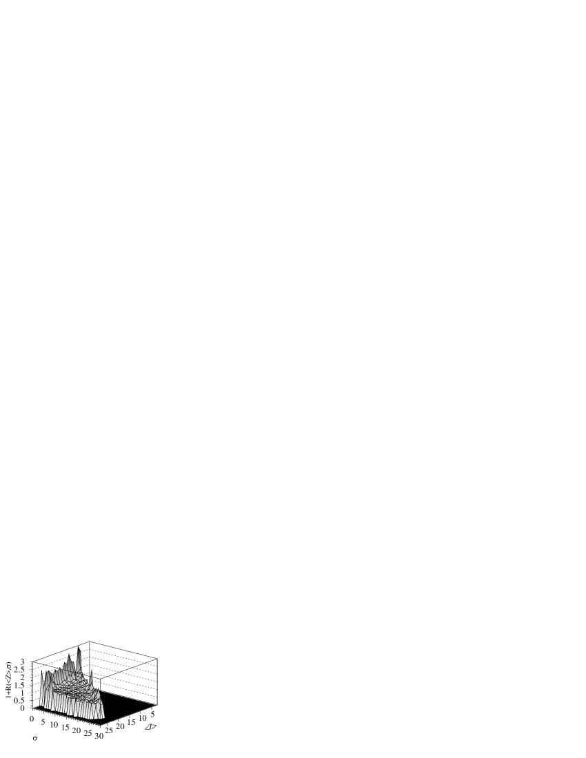
FIG. 12.: Brownian One Body model correlation function (same conventions as in Fig. 6.)

V Conclusions

The main goal of this article was to present a new method for the evaluation of the non trivial correlations between the fragment sizes of a finite size system. The conclusions are the following :

• The Monte-Carlo calculation of the denominator proposed by Moretto and collaborators can be replaced by a fast algebraic calculation which is equivalent to the selection of an infinite number of pseudo-events (10). This calculation results in decreased error bars in the correlation function notably those associated with correlation peaks (15). The extension of the calculation of the correlation function to samples including a variable number of imf presents no particular difficulty (12).

• Correlation functions thus obtained for the different models studied in this article (smm, percolation, minimum information, bob) all possess one maximum for $\langle Z\rangle$ smaller by a few units than $z_{\rm tot}/M$. This property leads to the evaluation of the size of the composite nuclei for which decays have been observed experimentally.

• This type of denominator possesses many advantages. However, correlations induced by charge conservation are always important. They may conceal other less trivial correlations, or distort the evaluation of their amplitude. It would, therefore, be useful to define a conventional method for calculation of the denominator including effects induced by the charge conservation.

• It has been proposed to evaluate the denominator using the minimum information model (all possible partitions of a given total charge has the same probability). This model incorporates charge conservation but possesses a purely combinatorial correlation peak at $\sigma=0$ so that there is a risk of concealing a physical peak present in the data sample (this effect can be corrected by the weighting of the partition probability by the number of its permutations : $m!/\prod_{z}n_{z}$). Furthermore, the numerator (physical sample) and denominator (given by this model) may correspond to distinct charge and multiplicity distributions. Finally, the correlation function presents numerous structures which are difficult to interpret.

• The two previous conclusions lead us to propose a new calculation of the denominator, the goal being to replicate all features of partitions of the numerator excluding intra-event correlations due to other reasons than charge conservation. In the case where these non trivial correlations are weak, this goal is reached exactly using the independent emission hypothesis constrained by the conservation of the charge. Probabilities of partitions are given by the formula (40) which is based on the specification of intrinsic probabilities for each charge. These values represent probabilities for a charge to be observed if the constraint of charge conservation played no role. The intrinsic probabilities are not observables, so that they must be searched for by a procedure of minimization between probabilities of partitions in the data sample and those given by the formula (40). If the resulting $\chi^{2}$ is low, it means that the studied sample is essentially composed of events corresponding to independent emission. The partition correlation function (i.e. the set of ratios of the probabilities of the sample divided by the probabilities given by Eq. (40)) must then be always near unity except possibly for a reduced number of partitions corresponding to the non trivial correlations. In this work, only the $[\langle Z\rangle,\sigma]$ correlation has been studied, but the same procedure can apply to any type of correlation.

• The proposed method has been applied to three models of nuclear multifragmentation. It has been shown that all three models correspond to almost independent emission. The first two (percolation and the smm statistical multifragmentation code) result in correlation functions everywhere equal to 1 (to within 10 %). The code bob, on the other hand, exhibits a flat correlation function everywhere except at $\sigma=0$. These correlation peaks are due to the mechanism of spinodal decomposition that favours partitions which include imf of the same charge. These results legitimate the use of the charge correlation functions method for the experimental search for spinodal decomposition.

In forthcoming articles we will study problems related to the application of this method to experimental event samples (superposition of sources , distribution of total charge, pre-equilibrium emission, experimental efficiency, calculation of the significance of the result) and we will present results obtained by the indra collaboration for heavy ion central collisions near the Fermi energy.

I wish to thank I.N. Mishustin who suggested this work, M.F. Rivet, B. Borderie and M. Parlog for numerous and fruitful discussions and A.J. Cole for precious advice concerning the manuscript.

Equations resulting from the utilization of the non-biaised estimator of the standard deviation

In this article, we used the usual definition of the standard deviation (3). The authors of Ref. [13] preferred to use the non-biased estimator (in this sense that the mean of its sampling function is equal to the real value). In writing this article, $\sigma$ being used as a measure and not as an evaluation of the standard deviation of an unknown distribution we restricted ourselves to its usual definition. In this Appendix we give the equations which result from the use of the non-biased value, $\sigma_{\rm nb}$ :

$$(\ref{Eq sigma usuel}) \rightarrow \sigma_{\rm nb}=\sqrt{\frac{1}{M-1}\ \sum_{i=1}^{M}(Z_{i}-\langle Z\rangle)^{2}}$$ (59)

$$(\ref{Eq p(s|m)}) \rightarrow P_{\rm uc}(\sigma_{\rm nb}|M)=\sum_{Z_{1}}\ldots\sum_{Z_{M-1}}$$ (63)

$$\times P_{Z}(Z_{1}|M)\ldots P_{Z}(Z_{M-1}|M)$$

$$\times P_{Z}(\langle Z\rangle^{\prime}+\sqrt{M\sigma_{\rm nb}^{2}-\frac{M(M-2)}{M-1}\sigma_{\rm nb}^{\prime 2}}\ |M)$$

$$\times P_{Z}(\langle Z\rangle^{\prime}-\sqrt{M\sigma_{\rm nb}^{2}-\frac{M(M-2)}{M-1}\sigma_{\rm nb}^{\prime 2}}\ |M)$$

$$(\ref{Eq P_Z(Z|m)}) \rightarrow P_{\rm uc}(\langle Z\rangle,\sigma_{\rm nb}\ |M)=\sum_{Z_{1}}\ldots\sum_{Z_{M}}$$ (67)

$$\times P_{Z}(Z_{1}|M)\ldots P_{Z}(Z_{M-1}|M)\ P_{Z}(Z_{M}|M)$$

$$\times\delta_{Z_{M},M\langle Z\rangle+(M-1)\langle Z\rangle^{\prime}}$$

$$\times\delta_{Z_{M},\langle Z\rangle^{\prime}\pm\sqrt{M\sigma_{\rm nb}^{2}-\frac{M(M-2)}{M-1}\sigma_{\rm nb}^{\prime 2}}}$$

$$(\ref{Eq multinomiale}) \rightarrow P_{\rm uc}(\langle Z\rangle,\sigma_{\rm nb}\ |M)\ =\ M!$$ (69)

$$\times\sum_{{{{\bf N}\atop\sum_{Z}N_{Z}=M}\atop\sum_{Z}ZN_{Z}=M\langle Z\rangle}\atop\sum_{Z}Z^{2}N_{Z}=M\langle Z\rangle^{2}+(M-1)\sigma_{\rm nb}^{2}}\ \prod_{Z}\frac{P_{Z}(Z|M)^{N_{Z}}}{N_{Z}!}$$

The other equations are not modified.

REFERENCES

-
[1]
L.G. Moretto, K. Tso, N. Colonna, G.J. Wozniak, Nucl. Phys. A545 (1992) 237c;
Phys. Rev. Lett. 69 (1992) 1884. - [2] W. Bauer, G.F. Bertsch and H. Schulz, Phys. Rev. Lett. 69 (1992) 1888.
- [3] B. Borderie, B. Remaud, M.F. Rivet and F. Sebille, Phys. Lett. B302 (1993) 15.
- [4] H.M. Xu et al., Phys. Rev. C048 (1993) 933.
-
[5]
A. Guarnera, M. Colonna and Ph. Chomaz, Phys. Let. B 373 (1996) 267,
Ph. Chomaz, M. Colonna, A. Guarnera and B. Jacquot, Nucl. Phys. A583 (1995) 305c. - [6] R.J. Charity et al., Nucl. Phys. A483 (1988) 371.
- [7] D. Durand, Nucl. Phys. A541 (1992) 266.
- [8] A.D. NGuyen, thesis, Université de Caen, LPCC T 9802 (1998).
- [9] J.P. Bondorf et al., Nucl. Phys. A443 (1985) 321.
-
[10]
G. Tăbăcaru et al. (indra collaboration), Communication to
the XXXVIII International Winter Meeting on Nuclear Physics, Bormio, Italy, ed.
by I. Iori, Ric. Sc. and E. P. (2000),
G. Tăbăcaru, Ph.D. thesis, Université Paris XI Orsay, (2000). - [11] D.H.E. Gross, Rep. Progr. Phys. 53 (1990) 605.
- [12] A. Le Fèvre, private communication.
-
[13]
L.G. Moretto et al., Phys. Rev. Let. 77 (1996) 2634,
L.G. Moretto et al., Phys. Rep. 287 (1997) 249. - [14] B. Borderie et al. (indra collaboration), Phys. Rev. Let. 86 (2001) 3252.
-
[15]
M. Bruno et al., Phys. Let. B292 (1992) 251,
M. Bruno et al., Nucl. Phys. A576 (1994) 138. - [16] D. Stauffer, ”Introduction to Percolation Theory”, Taylor and Francis, London (1985).
- [17] G. Tăbăcaru et al. (indra collaboration), in prep.
- [18] M. Abramowitz & I. Stegun, Handbook of Mathematical functions, NBS, Applied Math Series-55 (U.S. GPO, Washington, DC) (1965).
- [19] P. Désesquelles, submitted to Phys. Rev. C.
- [20] L.G. Sobotka and L. G. Moretto, Phys. Rev. C31 (1985) 668.
-
[21]
J. Aichelin and J. Huefner, Phys. Let. B136 (1984) 15,
J. Aichelin et al., Phys. Rev. C30 (1984) 107. - [22] A.S. Botvina, A.D. Jackson and I. Mishustin, Phys. Rev. E62 (2000) R64.
-
[23]
A.R. DeAngelis and A.Z. Mekjian, Phys. Rev. C40 (1989) 105,
A.Z. Mekjian, Phys. Rev. Lett. 64 (1990) 2125,
A.Z. Mekjian, Phys. Rev. C41 (1990) 2103. -
[24]
A.J. Cole and P. Désesquelles, Z. Phys. A337 (1990) 71,
A.J. Cole and P. Désesquelles, Phys. Rev. C50 (1994) 329,
A.J. Cole et al., Z. Phys. A356 (1996) 171. - [25] B. Guiot et al. (indra collaboration), in prep.
-
[26]
J.P. Bondorf, R. Donangelo, I.N. Mishustin, H. Schulz, Nucl. Phys. A444 (1985)
460,
J.P. Bondorf, A.S Botvina, A.S. Iljinov, I.N. Mishustin, K. Sneppen, Phys. Rep. 257 (1995) 133. -
[27]
J.D. Frankland, PhD Thesis, Orsay, IPNO T 98-06 (1998),
J.D. Frankland et al. (indra collaboration), Nucl. Phys. A689 (2001) 905,
Nucl. Phys. A689 (2001) 940. - [28] A. Bonasera, F. Gulminelli and J. Molitoris, Phys. Rep. 243 (1994) 1.
- [29] M. Bixon and R. Zwanzig, Phys. Rev. 187 (1969) 267.
- [30] D. Cussol, indra filter, private communication.