Compton Scattering by the Proton using a Large-Acceptance Arrangement

Abstract

Compton scattering by the proton has been measured over a wide range covering photon energies $250~{}\mathrm{MeV}\lesssim E_{\gamma}\lesssim 800~{}~{}\mathrm{MeV}$ and photon scattering angles $30^{\circ}\lesssim\theta^{\mathrm{lab}}_{\gamma}\lesssim 150^{\circ}$, using the tagged-photon facility at MAMI (Mainz) and the large-acceptance arrangement LARA. The previously existing data base on proton Compton scattering is greatly enlarged by more than 700 new data points. The new data are interpreted in terms of dispersion theory based on the SAID-SM99K parametrization of photo-meson amplitudes. It is found that two-pion exchange in the $t$-channel is needed for a description of the data in the second resonance region. The data are well represented if this channel is modeled by a single pole with the mass parameter $m_{\sigma}\approx$ 600 MeV. The asymptotic part of the spin dependent amplitude is found to be well represented by $\pi^{0}$-exchange in the $t$-channel. No indications of additional effects were found. Using the mass parameter $m_{\sigma}$ of the two-pion exchange determined from the second resonance region and using the new global average for the difference of the electric and magnetic polarizabilities of the proton, $\alpha-\beta=\left(10.5\pm 0.9_{\mathrm{stat+syst}}\pm 0.7_{\mathrm{model}}\right)\times 10^{-4}~{}\mathrm{fm}^{3}$, as obtained from a recent experiment on proton Compton scattering below pion photoproduction threshold, a backward spin-polarizability of $\gamma_{\pi}=\left(-37.1\pm 0.6_{\mathrm{stat+syst}}\pm 3.0_{\mathrm{model}}\right)\times 10^{-4}~{}\mathrm{fm}^{4}$ has been determined from data of the first resonance region below 455 MeV. This value is in a good agreement with predictions of dispersion relations and chiral perturbation theory. From a subset of data between 280 and 360 MeV the resonance pion-photoproduction amplitudes were evaluated leading to a E2/M1 multipole ratio of the p $\to$ $\Delta$ radiative transition of EMR(340 MeV)= $(-1.7\pm 0.4_{\rm stat+syst}\pm 0.2_{\rm model})$%. It was found that this number is dependent on the parameterization of photo-meson amplitudes. With the MAID2K parameterization an E2/M1 multipole ratio of EMR(340 MeV)= $(-2.0\pm 0.4_{\rm stat+syst}\pm 0.2_{\rm model})$% is obtained.

1 Introduction

Elastic scattering of photons from the proton (proton Compton scattering) is known baranov76 ; petrunkin81 to be a valuable tool for investigations of the structure of the nucleon. The specific feature of this process is that it depends on the electromagnetic interaction only and, therefore, is especially suited to study electromagnetic properties of the nucleon. Nevertheless, it took a long time until decent use could be made of the method. One reason for the delay was that the process is difficult to measure and, therefore, the data base remained fragmentary. The other reason was that the methods of data interpretation were not well enough developed, so that definite conclusions on the electromagnetic properties of the nucleon could not be drawn with the desired precision. The present work shows that by now the shortcomings of the previous approaches have been overcome due to new experimental techniques applied here for the first time in a Compton scattering experiment and due to recent and continuing progress in developing the dispersion theory of Compton scattering.

The properties of the nucleon accessible by a given experiment depend on the type of the reaction. In Compton scattering properties are selected which are specific for two-photon interactions. These are the electromagnetic polarizabilities and spin polarizabilities in first place and specific $t$-channel exchanges. Furthermore, due to the optical theorem and dispersion relations there is a close relation to meson photoproduction. This implies that Compton scattering also is a good tool of nucleon spectroscopy for measurements of strengths and multipolarities of electromagnetic transitions.

An exhaustive review of literature on proton Compton scattering in the energy region of nucleon resonances up to 1974 has been published by Baranov and Fil’kov baranov76 . Shortly thereafter experiments have been carried out in Bonn genzel76 ; jung81 and Tokyo ishii80 ; wada84 which led to essential progress. The main difficulty in measuring Compton scattering by the proton above the meson photoproduction threshold consists in the separation of the ($\gamma$,$\gamma$) from the ($\gamma$,$\pi^{0}$) reaction channel. This difficulty has led to different strategies depending on the available photon facility and the detection system. Because of the absence of high duty-factor electron beams and connected with that, the absence of high fluxes of tagged photons, the previous experiments had to be carried out with bremsstrahlung genzel76 ; jung81 ; ishii80 ; wada84 . As long as the experiments were restricted to the $\Delta$ energy range genzel76 scintillator telescopes for the proton and the detection of the shower produced by the photon were sufficient. At higher energies jung81 ; ishii80 ; wada84 the lack of information on the energy of the primary photon had to be compensated by high-resolution proton spectrometry which required the use of magnetic spectrometers in combination with high angular-resolution track reconstruction. By achieving also a good position resolution of the photon it was then possible to measure $p-\gamma$ directional correlations with high angular resolution. In the Bonn set-up jung81 a large-volume NaI(Tl) detector was used with photomultipliers on the front side to locate the incidence point of the photon. In the Tokyo set-up ishii80 ; wada84 a lead glass Čerenkov counter was used in combination with a lead plate $\gamma\to e^{+}e^{-}$ converter and two multi-wire proportional chambers. When applying this method, the events from the two reaction channels $(\gamma,\gamma)$ and $(\gamma,\pi^{0})$ differ in the widths of the $p-\gamma$ angular correlations. Therefore, the $(\gamma,\gamma)$ events show up as a narrow peak on top of a broad background. Though this method leads to a comparatively safe separation of events, it has the disadvantage that one setting of the apparatus leads to only one differential cross section per given angular and energy interval.

At modern facilities with tagged photons experiments providing only one differential cross section per given angular and energy interval are not in line with the required economic use of the beam. When using tagged photons together with a large-volume NaI(Tl) detector it is relatively easy to separate the two types of events through the good energy resolution of the NaI(Tl) detector over the whole energy range of the $\Delta$ resonance. This method has been applied in Compton scattering experiments by the proton carried out at the tagged-photon facilities at Saskatoon (SAL) hallin93 , Brookhaven (LEGS) blanpied96 ; blanpied97 ; tonnison98 and Mainz (MAMI) peise96 ; huenger97 ; wissmann99 . The advantage of this method is that the recoil proton has not necessarily to be detected, so that there is no restriction in the accessibility of small photon angles and low photon energies, where the recoil proton does not leave the target with sufficiently high energy to reach the detector. The disadvantages are the restriction to the $\Delta$ energy range and the accessibility of only one scattering angle per beam-time period. In an other experiment carried out at MAMI (Mainz) molinari96 the apparatus determined the full set of kinematical variables of the photon and the proton. The protons were detected using an $E$–$\Delta E$ plastic scintillator telescope the photons were registered by lead glass detectors.

The LARA (LARge Acceptance) experiment is the first Compton scattering experiment where the restrictions discussed above were overcome and a large angular range from $\theta^{\mathrm{lab}}_{\gamma}=30^{\circ}$ to $150^{\circ}$ and large energy range from E_γ = 250 MeV to 800 MeV is covered simultaneously with one experimental set-up. This is achieved by the use of the tagging method in combination with large acceptance arrangements for the recoil proton and the scattered photon. In principle, the apparatus determines the full set of kinematical variables of the proton and the photon and contains many features of the Bonn jung81 and Tokyo ishii80 ; wada84 designs, except for the fact that magnetic spectrometers are incompatible with large angular and energy acceptance detection. Therefore, the proton spectrometry had to rely on time-of-flight measurements using long flight paths. Except for the available space, the limitations of this method are given by the energy loss and the straggling of the protons in air. Due to straggling the proton angle cannot be determined to much better than $\Delta\theta_{\mathrm{p}}=\pm 1^{\circ}$ corresponding to a photon interval of $\Delta\theta_{\gamma}=\pm 2^{\circ}$ for the Compton kinematics. This was the underlying point of view when selecting the angular resolutions for the photons and protons in the apparatus design. The expected properties of the LARA experimental set-up have been explored in detailed simulation studies falkenberg95 . In these studies it was shown that by combining $p-\gamma$ angular correlation with time of flight measurements an event by event separation of $(\gamma,\gamma)$ and $(\gamma,\pi^{0})$ events should be possible in the energy region of the first resonance and that this property should be partly preserved in the second resonance region.

The dispersion theory of Compton scattering by the nucleon which formerly was restricted to the first resonance baranov76 ; pfeil74 ; guiasu78 ; akhmedov81 ; lvov81 ; lvov85 has been extended to cover also the second resonance region lvov97 . This dispersion theory proved to be much more precise than alternative approaches based on a phenomenological resonance model ishii80 ; wada84 , where the scattering amplitude is represented as a sum of Breit-Wigner nucleon resonances and an adjusted real background which is assumed to be a modified Born term. Even after the development of improved resonance models, in which a K-matrix unitarization is implemented hida76 ; feuster99 ; korchin98 ; korchin00 , the dispersion theory still provides the highest precision.

The quantitative success of the dispersion theory supports the expectation that Compton scattering may be used as a precise tool for measuring several electromagnetic properties of the nucleon, including in particular the electric and magnetic polarizabilities $\alpha$ and $\beta$, the four so-called spin polarizabilities $\gamma_{i}$ (the backward spin polarizability $\gamma_{\pi}$ being a particular linear combination of them), the strength $M_{1+}$ and the multipole ratio E2/M1 of the $N\to\Delta$ transition. These quantities enter into the theoretical Compton differential cross section as (not fully independent) parameters and they are predominantly important in the $\Delta$ energy range.

The dispersion theory described in lvov97 has recently been improved in some aspects by Drechsel et al. drechsel99 using subtracted dispersion relations. The main difference of the recent version drechsel99 compared to the former one lvov97 is that, like in guiasu78 ; akhmedov81 and some older works, the two-pion $t$-channel exchange was implemented in an explicit way in order to fix otherwise uncertain so-called asymptotic contributions to the invariant amplitudes $A_{1}$ and $A_{2}$. Theoretically such an improvement is very important because it has the potential to remove free parameters which are specific for nucleon Compton scattering. Practically, however, free parameters do not disappear completely, since the $t$-channel exchanges are not exhausted by low-lying $\pi^{0}$ and $\pi\pi$ states. Thus, a poorly-known input from high-energy contributions actually remains in the theory.

The difference between the two versions of the dispersion theory have been found by us to be small in the $\Delta$ energy range but still have to be explored for higher energies where at present no predictions from subtracted dispersion relations are available.

The dispersion theory in the version of L’vov et al. lvov97 utilizes a less sophisticated phenomenological approach for a description of $t$-channel exchanges. In the formalism of unsubtracted fixed-$t$ dispersion relations used there, these are the asymptotic contributions $A_{i}^{\rm as}(\nu,t)$ which carry the information on $t$-channel exchanges. These contributions are theoretically expected to be energy independent at energies $E_{\gamma}$ well below the cutoff $E_{\gamma}^{\mathrm{max}}\approx 1.5$ GeV used for separating the asymptotic region. Therefore, only a $t$-dependence of $A_{i}^{\rm as}(\nu,t)$ is taken into account. Practically, these amplitudes are parameterized by pole $t$-channel exchanges associated with the lightest mesons. In particular, the asymptotic contribution $A_{1}^{\rm as}$ is parameterized by an effective $\sigma$-exchange which therefore introduces an adjustable parameter, $m_{\sigma}$, which can be loosely interpreted as a (effective) mass of the $\sigma$ meson. The product of couplings of the $\sigma$ meson to the photon and the nucleon constitutes one additional parameter, which is fixed using an experimental number for the difference, $\alpha-\beta$, of the electric and magnetic polarizabilities of the proton.

One other large asymptotic contribution, $A_{2}^{\rm as}$, is assumed to be given by $\pi^{0}$-exchange. An important question raised by Tonnison et al. tonnison98 is, whether the $\pi^{0}$-exchange indeed exhausts the asymptotic contribution to the amplitude $A_{2}$ or, alternatively, an additional large background exists in $t$-channel exchanges with the quantum numbers of pseudoscalar mesons. In the latter case, such a background can largely modify the backward spin polarizability of the proton, $\gamma_{\pi}$, which therefore becomes an important signature of the $t$-channel dynamics of Compton scattering.

Another feature of the theory lvov97 is that it takes into account an important channel of double-pion photoproduction including $\pi\Delta$-production. In forward direction the contribution of the $2\pi$-channel to the Compton scattering amplitude is well known. Its extension to nonforward angles requires a further consideration of the multipole structure of double-pion photoproduction (see lvov97 for details). The result may then be tested by experiments carried out in the second resonance region.

The present paper contains an exhaustive description of the results of the LARA experiment and their interpretation in terms of the currently accepted dispersion theory lvov97 based on the SAID-SM99K arndt96 multipole analysis and specific models to take into account asymptotic contributions or subtractions. For comparison also the MAID2K maid parameterization has been applied. A short version of this work has been published elsewhere galler01 .

In contrast to our present approach, the realistic $2\pi$-exchange in the $t$-channel does not correspond to a narrow resonance but rather to a broad continuum. This apparent deficiency of our approach does not show up as a discrepancy when comparing the present experimental data with predictions. However, from a theoretical point of view this deficiency is not acceptable and should be removed. This will be done in a following paper which is devoted to improvements of the dispersion theory and to further interpretations.

2 Experiment

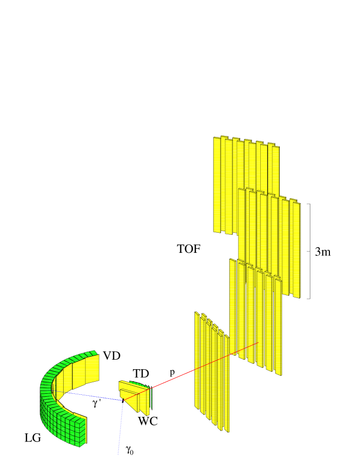
Figure 1: Perspective view of the LARA arrangement. Left: Photon arm consisting of 10 blocks à 3 $\times$ 5 lead glass detectors (LG) each block equipped with a 1 cm plastic scintillator (VD). Right: Proton arm consisting of two wire chambers (WC) at distances of 25 and 50 cm from the target center, 8 plastic scintillators serving as trigger detectors (TD) and 43 bars of 20 cm $\times$ 300 cm $\times$ 5 cm plastic scintillators serving as time-of-flight (TOF) stop detectors. The scattering target consisted of lq. $\mathrm{H}_{2}$ contained in a 3 cm $\varnothing$ $\times$ 20 cm Kapton cylinder.

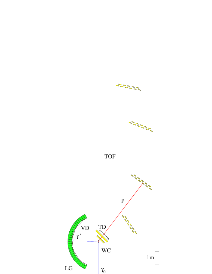
Figure 2: Same as Figure 1 but projected into the horizontal plane

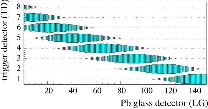
Figure 3: Simulated scatter plot of events showing the correlation between trigger detector (TD) and Pb glass detectors (LG) for Compton events. Abscissa: Number of the Pb glass detector with the detectors 1–5 covering the angular range from $\theta^{\mathrm{lab}}_{\gamma}=25^{\circ}$ to $30^{\circ}$ and the detectors 146–150 covering the angular range from $\theta^{\mathrm{lab}}_{\gamma}=150^{\circ}$ to $155^{\circ}$. The trigger detector 1 is closest to the forward direction and covers the range of proton angles from $\theta^{\mathrm{lab}}_{\mathrm{p}}=7.3^{\circ}$ to $15.6^{\circ}$. The correlation between the two angles $\theta^{\mathrm{lab}}_{\gamma}$ and $\theta^{\mathrm{lab}}_{\mathrm{p}}$ was used to preselect Compton events through the trigger condition.

The present paper contains the results of an experiment carried out using the LARge Acceptance arrangement (LARA) shown in Fig. 1 as a perspective view from the side. The same apparatus is shown in Fig. 2 as viewed from the top. This arrangement was designed to cover the angular range of photon scattering-angles from $\theta^{\mathrm{lab}}_{\gamma}=30^{\circ}$ to $150^{\circ}$ in the laboratory and the interval of photon energies from E_γ = $250\;\mathrm{MeV}$ to $800\;\mathrm{MeV}$ with limitations given by the range of protons in the scattering target. Due to the energy loss in the scattering target the minimum energy of a proton to be detected is about 30 MeV. This leads to the unwanted restriction that the small-angle low-energy section of the photon range given above is not accessible. However, this range should easily be accessible by an experiment with a large-volume NaI(Tl) detector like the Mainz 48 cm $\varnothing$ $\times$ 64 cm NaI(Tl) detector huenger97 . This detector has sufficient energy resolution in this range to separate photons from the $(\gamma,\gamma)$ and $(\gamma,\pi^{0})$ reactions so that the recoil protons have not to be detected.

The experiment makes use of the tagged photon facility anthony91 installed at the $855\;\mathrm{MeV}$ three-stage microtron MAMI in Mainz herminghaus76 . The energy resolution achieved by the tagger was $\Delta E_{\gamma}=2\;\mathrm{MeV}$ on the average. The maximum rate of tagged photons as limited by the tagger is $10^{5}\;\mathrm{s}^{-1}$ per tagger channel. In the present case this rate was lower by a factor of about two because of limitations due to the wire chambers.

The scattering target consists of lq. $\mathrm{H}_{2}$ contained in a Kapton cylinder of $200\;\mathrm{mm}$ length and $30\;\mathrm{mm}$ diameter. The apparatus (Figs. 1 and 2) consists of 150 lead glass photon detectors (LG) having dimensions of $15\;\mathrm{cm}\times 15\;\mathrm{cm}\times 30\;\mathrm{cm}$ positioned cylindrically around the scattering target with the front faces having distances of $200\;\mathrm{cm}$ from the target center. This leads to an angular resolution on the photon arm of $\pm 2.2^{\circ}$ both in the horizontal and the vertical direction. Each block containing 3 (horizontal) $\times$ 5 (vertical) detectors is equipped with a plastic scintillator (VD) of $1\;\mathrm{cm}$ thickness to identify charged background.

On the proton arm of the detector arrangement the proton angle $\theta_{\mathrm{p}}$ with respect to the incident photon beam is determined by two wire chambers (WC) at distances of $25\;\mathrm{cm}$ and $50\;\mathrm{cm}$ from the target center. Each of these wire chambers consists of two layers of wires tilted against the vertical direction by $+30^{\circ}$ and $-30^{\circ}$, respectively. The distance between wires in the layers is 2.5 mm. The resolution achieved for the proton angle is better than $1^{\circ}$ in the horizontal (geometrical $0.13^{\circ}$) and vertical (geometrical $0.47^{\circ}$) directions. The time of flight is measured through coincidences between signals from the tagger and signals from 43 bars of $20\;\mathrm{cm}\times 300\;\mathrm{cm}\times 5\;\mathrm{cm}$ plastic scintillators (TOF) grabmayr98 . The latter are arranged in 4 planes positioned at distances of 2.6, 5.7, 9.4 and $12.0\;\mathrm{m}$ from the target center. The experiment trigger was defined through a coincidence between a signal from a lead glass block and a signal from one out of 8 trigger detectors (TD) positioned behind the wire chambers, with the geometry complying with the angular constraints of a Compton event. The preselection of data possible through the trigger condition is demonstrated in Fig. 3, where the correlation between the trigger detectors and the Pb glass detectors is shown by a scatter plot of events obtained by computer simulation. Each 5 of the 150 Pb glass detectors are positioned on top of each other so that ranges of 5 successive Pb glass detectors approximately correspond to the same interval of photon scattering angles.

3 Data analysis

Figure 4: Typical experimental missing time spectra for protons at primary photon energies of $E_{\gamma}=345.3$ MeV (upper figure) and $E_{\gamma}=413.0$ MeV (lower figure) measured at a photon angle of $\theta^{\mathrm{lab}}_{\gamma^{\prime}}=70^{\circ}$. The protons were detected with one plastic scintillator bar positioned at a proton angle of $\theta^{\mathrm{lab}}_{\mathrm{p}}=45^{\circ}$.

Figure 5: Typical experimental missing time spectrum for protons at a primary photon energy of $E_{\gamma}=659.3$ MeV measured at a photon angle of $\theta^{\mathrm{lab}}_{\gamma^{\prime}}=116^{\circ}$. The protons were detected with 4 plastic scintillator bars positioned around a proton angle of $\theta^{\mathrm{lab}}_{\mathrm{p}}=20^{\circ}$. A: In-plane data. B: Out-of-plane data. C: In-plane data and the corresponding adjusted out-of-plane data (cross-hatched area). D: Compton events obtained from the in-plane data by subtracting the corresponding adjusted out-of-plane data.

Figure 6: Two-dimensional analysis of experimental data obtained at a photon energy of $E_{\gamma}=467.4$ MeV and a scattering angle of $\theta^{\mathrm{lab}}_{\gamma}=37^{\circ}$. The data were obtained with 4 TOF plastic scintillator bars positioned at proton angles around $\theta^{\mathrm{lab}}_{\mathrm{p}}=63^{\circ}$. A: Scatter plot of experimental data measured in-plane. B: Scatter plot of experimental data measured out-of-plane. In these two subfigures the rectangular frames denote those ranges where Compton events are expected to be located in A. C: Vertical projection of the data inside the rectangular frames, with the data from A denoted by full lines and the corresponding out-of-plane data denoted by a dashed lines. D: Same as C but showing the difference between the solid and the dashed lines. E: Horizontal projection of the data inside the rectangular frames, with the data from A denoted by full lines and the corresponding out-of-plane data denoted by a dashed lines. F: Same as E but showing the difference between the solid and the dashed lines.

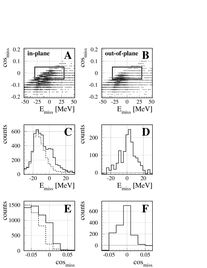
Figure 7: Two-dimensional analysis of experimental data obtained at a photon energy $E_{\gamma}=657.5$ MeV and a scattering angle of $\theta^{\mathrm{lab}}_{\gamma}=29^{\circ}$. The data were obtained with 4 TOF plastic scintillator bars positioned at proton angles around $\theta^{\mathrm{lab}}_{\mathrm{p}}=67^{\circ}$. For further details see Fig. 6.

Figure 8: Two-dimensional analysis of experimental data obtained at a photon energy $E_{\gamma}=779.9$ MeV and a scattering angle of $\theta^{\mathrm{lab}}_{\gamma}=32^{\circ}$. The data were obtained with 4 TOF plastic scintillator bars positioned at proton angles around $\theta^{\mathrm{lab}}_{\mathrm{p}}=62^{\circ}$. For further details see Fig. 6.

Protons were identified through their comparatively large energy-deposition in a TD detector and through their time-of-flight. For each proton event detected by a TOF detector a trajectory was constructed using the intersection points in the two wire chambers. The event was accepted as a good one if the trajectory intersected the scattering target, hit the appropriate TD detector and intersected the TOF detector at the experimental impact point within its spatial resolution. Then, for a given proton trajectory and a given primary photon energy $E_{\gamma}$ the direction $\theta^{\mathrm{Comp}}_{\gamma}$ and energy $E^{\mathrm{Comp}}_{\gamma}$ of the secondary photon as well as the energy $E^{\mathrm{Comp}}_{\mathrm{p}}$ of the recoil proton were calculated assuming Compton kinematics. Only those events were accepted where the experimental direction of the secondary photon was close to the direction calculated for a Compton photon. This procedure led to a drastic reduction of the number of background events from $\pi^{0}$ photoproduction.

The final separation of events from Compton scattering and $\pi^{0}$ photoproduction was achieved by time-of-flight analysis. The experimental time-of-flight was compared with the one calculated from the energy $E^{\mathrm{Comp}}_{\mathrm{p}}$ expected for a recoil proton of a Compton event. Mean energy losses of the proton were used in this calculation. The difference between the experimental and the calculated time-of-flight was named the missing time $\Delta t_{\mathrm{p}}$.

Figs. 4 and 5 show typical missing time spectra for incident photon energies of $E_{\gamma}$ = 345.3 MeV, 413.0 MeV and 659.3 MeV, the former two for intermediate photon angle of $\theta^{\mathrm{lab}}_{\gamma}=70^{\circ}$ and the latter for a large photon angle of $\theta^{\rm lab}_{\gamma}=116^{\circ}$. The corresponding proton angles were $\theta^{\mathrm{lab}}_{\mathrm{p}}=45^{\circ}$ and $20^{\circ}$, respectively. These three cases were selected to demonstrate examples of “comparatively easy” separation of events from the $(\gamma,\gamma)$ and $(\gamma,\pi^{0})$ reactions. At the lowest energy of $E_{\gamma}$ = 345.3 MeV there is a complete separation of the two types of events, whereas at the higher energy of $E_{\gamma}$ = 413.0 MeV there is some overlap which can be removed by subtracting the tail of the $(\gamma,\pi^{0})$ events underneath the $(\gamma,\gamma)$ events. The shape of this tail was taken from the out-of-plane data. At the higher energy of $E_{\gamma}$ = 659.3 MeV the overlap of the two types of events is complete. However, after using the appropriate cuts the remaining background of $(\gamma,\pi^{0})$ events is considerably smaller than the corresponding number of $(\gamma,\gamma)$ events. This made the separation of the two types of events precise and comparatively easy. In this case the background due to $(\gamma,\pi^{0})$ events was taken from experimental data where the photon was detected outside the Compton scattering plane. These out-of-plane data were then transferred into the Compton scattering plane by help of the predictions of a computer simulation. This method was already successfully applied in one of the previous experiments carried out in Mainz molinari96 . The validity of this method was clearly demonstrated in Refs. molinari96 and huenger97 .

To determine the detector efficiencies the analysis of the experimental data was accompanied by a Monte Carlo simulation taking into account all relevant effects. All calibrations needed as inputs for a precise simulation, including the efficiencies of the wire chambers, were found in a self-calibration procedure making use of the large amount of data from the ($\gamma,\pi^{0}$) reaction.

In a second analysis of the data of the second resonance region carried out independently of the one described above, the one-dimensional analysis in terms of the missing time $\Delta t_{\mathrm{p}}$ was replaced by a two-dimensional analysis with $\Delta t_{\mathrm{p}}$ – or the equivalent missing energy E_miss – and the difference $\cos_{\mathrm{miss}}$ between the experimental $\cos\theta_{\gamma}$ and $\cos\theta^{\mathrm{Comp}}_{\gamma}$ as the two coordinates. The two dimensional procedure is illustrated in Figs. 6–8 corresponding to a small photon angle in the range of $\theta^{\mathrm{lab}}_{\gamma}$ = 28^∘–37^∘ where the separation of the two types of events is “comparatively difficult”. The two upper subfigures (A) and (B) show scatter plots of events, with the photon detected in the Compton scattering plane and outside the Compton scattering plane, respectively. The rectangular frames are chosen such that for the in-plane data (subfigures (A)) Compton events are entirely located in this frame. By comparing the Figs. 6–8 with each other we notice that the peaks of the $(\gamma,\pi^{0})$ distributions are outside the rectangular frames at the lowest photon energy and are moving into the center of the rectangular frames at the highest photon energy. This is in line with the expectation that with increasing photon energy effects of the finite pion mass become less important. As before, the background from $\pi^{0}$ photoproduction was obtained from the out-of-plane data and subtracted from the in-plane data. For this procedure the scatter plots of $(\gamma,\pi^{0})$ events in the two upper parts of Figs. 6–8 were also generated by a Computer simulation and adjusted to the corresponding experimental data outside the rectangular frames. These adjusted simulated data were then used to correct for possible differences in the experimental $(\gamma,\pi^{0})$ data located in the rectangular frames of the subfigures (A) and (B). In subfigures (C) to (F) projections of the data located inside the rectangular frames on the $E_{\mathrm{miss}}$ and $\cos_{\mathrm{miss}}$ axes, respectively, are shown. In the subfigures (C) and (E) the solid curves represent $(\gamma,\gamma)$ plus $(\gamma,\pi^{0})$ events (in-plane data) and the dashed curves the $(\gamma,\pi^{0})$ background (out-of-plane data). The curve in the subfigures (D) and (F) show the net number of $(\gamma,\gamma)$ events. The projections in the subfigures (C) to (F) of Figs. 6–8 are shown for illustration, whereas the differential cross sections for Compton scattering have been derived by directly evaluating the contents of the rectangular frames of the upper subfigures (A) and (B). This two-dimensional analysis extended the available differential cross sections to smaller scattering angles as compared to the one-dimensional analysis. The results nicely agree with those from the one-dimensional analysis in the regions where both types of analyses have been carried out.

The procedures described above led to data with individual (random) errors which have been carefully determined during the evaluation procedure. These random errors are due to the counting statistics and the systematic errors due to the detection efficiency, the geometrical uncertainty of the apparatus and of the background-subtraction procedure. There are additional common (scale) systematic errors due to the tagging efficiency $(\pm 2\%)$ and target density and thickness $(\pm 2\%)$. The scale errors of the quantities extracted from our data were obtained by scaling all data points to 97% and 103% of their nominal values. Since the random errors contain statistical and systematic components we do not discriminate between these two types of errors in the results presented in the following. The combined statistical+systematic errors have been obtained by adding random and scale errors in quadrature.

The number of differential cross sections obtained for the first resonance region below 455 MeV is 436. With the two different analyses a total number of 329 differential cross sections has been obtained for the second resonance region above 455 MeV. Of these 221 are partly overlapping with respect to the energy and angular range. This overlap has carefully been taken into account in the determination of the number of degrees of freedom (d.o.f.) used in the $\chi^{2}$ procedures described in the following. Since it appeared inappropriate to combine two data points from only partly overlapping intervals into one data point by averaging, the following procedure was applied. The two data points were kept separate but their individual errors were enlarged by a factor of $\sqrt{2}$, giving a hypothetical arithmetic average the same error as the single data points have.

The differential cross sections obtained in the present experiment are given in Tables LABEL:tab:tab1 to LABEL:tab:tab3 shown in the appendix.

4 Theory

In the general case Compton scattering is described by six invariant amplitudes $A_{i}(\nu,t)$, $i=1\cdots 6$ lvov97 where

$$\nu = \frac{s-u}{4m}=E_{\gamma}+\frac{t}{4m},\quad t=(k-k^{\prime})^{2},\quad s=(k+p)^{2},$$

$$u = (k-p^{\prime})^{2}$$ (1)

and $s+u+t=2m^{2}$. These amplitudes can be constructed to have no kinematical singularities and constraints and to obey the usual dispersion relations. We formulate fixed-$t$ dispersions relations for $A_{i}(\nu,t)$ by using a Cauchy loop of finite size (a closed semicircle of radius $\nu_{max}$), so that

$${\rm Re}A_{i}(\nu,t)=A^{\rm pole}_{i}(\nu,t)+A^{\rm int}_{i}(\nu,t)+A^{\rm as}_{i}(\nu,t)$$ (2)

with

$$A^{\rm pole}_{i}(\nu,t) = \frac{a_{i}(t)}{\nu^{2}-t^{2}/16m^{2}}$$

$$A^{\rm int}(\nu,t) = \frac{2}{\pi}{\cal P}\int^{\nu_{\rm max}(t)}_{\nu_{\rm thr}(t)}{\rm Im}A_{i}(\nu^{\prime},t)\frac{\nu^{\prime}d\nu^{\prime}}{{\nu^{\prime}}^{2}-\nu^{2}}$$

$$A^{\rm as}(\nu,t) = \frac{1}{\pi}{\rm Im}\int_{{\cal C}_{\nu_{\rm max}}}A_{i}(\nu^{\prime},t)\frac{\nu^{\prime}d\nu^{\prime}}{{\nu^{\prime}}^{2}-\nu^{2}}.$$ (3)

The explicit use of the contour integral for $A^{\rm as}(\nu,t)$ is only necessary for i = 1 and 2, where special models have to be used for this purpose. For i = 3 $\cdots$ 6 the contour integral for $A^{\rm as}(\nu,t)$ can be avoided by extending the integral for $A^{\rm int}(\nu,t)$ to infinity.

The integral contributions $A^{\rm int}_{i}(\nu,t)$ are determined by the imaginary part of the Compton scattering amplitude which is given by the unitarity relation of the generic form

$$2{\rm Im}T_{fi}=\sum_{n}(2\pi)^{4}\delta^{4}(P_{n}-P_{i})T^{*}_{nf}T_{ni}.$$ (4)

The quantities entering into the r.h.s. of (4) are from $n=\pi N$ and $n=2\pi N$ intermediate states where the $n=\pi N$ component can be constructed from parameterizations of pion photoproduction multipoles $E_{l\pm}$, $M_{l\pm}$. The $n=2\pi N$ component requires additional model considerations lvov97 .

For the asymptotic part of the amplitude $A_{2}(\nu,t)$ we may use the Low amplitude of the $\pi^{0}$ exchange in the $t$-channel

$$A^{\rm as}_{2}(t)\simeq A^{\pi^{0}}_{2}(t)=\frac{g_{\pi NN}F_{\pi^{0}\gamma\gamma}}{t-m^{2}_{\pi^{0}}}\tau_{3}F_{\pi}(t),$$ (5)

where the isospin factor is $\tau_{3}=\pm 1$ for the proton and neutron, respectively, and the product of the $\pi NN$ and $\pi^{0}\gamma\gamma$ couplings is

$$g_{\pi NN}F_{\pi^{0}\gamma\gamma} = -16\pi\sqrt{\frac{g^{2}_{\pi NN}}{4\pi}\frac{\Gamma_{\pi^{0}\to 2\gamma}}{m^{3}_{\pi^{0}}}}$$ (6)

$$= (-0.331\pm 0.012)\,{\rm GeV}^{-1}.$$

The inclusion of small corrections due to the $\eta$ and $\eta^{\prime}$ mesons has been described elsewhere lvov99 . There may be arguments that $A^{\rm as}_{2}(t)$ is not exhausted by $\pi^{0}$ exchange in the $t$-channel. In order to introduce an additional parameter into the relevant amplitude which provides the necessary flexibility for an experimental test we write

$$A^{\rm as}_{2}(t)\simeq A^{\pi^{0}}_{2}(t)-2\pi m\frac{\delta\gamma_{\pi}}{1-\frac{t}{\Lambda^{2}}}$$ (7)

from which the substitution follows:

$$\gamma_{\pi}\to\gamma_{\pi}+\delta\gamma_{\pi}.$$ (8)

The parameter $\Lambda$ defines the slope of the function at $t=0$ and is chosen to be $\Lambda$ = 700 MeV. In varying $\delta\gamma_{\pi}$ the influence of any deviation from the standard value of $\gamma_{\pi}$ can be investigated in terms of this ansatz.

The asymptotic contribution of the amplitude $A_{1}(\nu,t)$ is modeled through an ansatz analogous to the Low amplitude, except for the fact that the pseudoscalar meson $\pi^{0}$ is replaced by the scalar $\sigma$ meson. In this case we use a simpler form of the ansatz

$$A^{\rm as}_{1}(t)\simeq A^{\sigma}_{1}(t)=\frac{g_{\sigma NN}F_{\sigma\gamma\gamma}}{t-m^{2}_{\sigma}}$$ (9)

and include quantities like the formfactor in (5) into the ”effective mass” $m_{\sigma}$ being now an adjustable parameter lvov97 ; galler01 . The quantity $g_{\sigma NN}F_{\sigma\gamma\gamma}$ is given by the difference of the electric and magnetic polarizabilities $\alpha-\beta$ through

$$2\pi(\alpha-\beta)+A^{\rm int}_{1}(0,0)=-A^{\rm as}_{1}(0,0)=\frac{g_{\sigma NN}F_{\sigma\gamma\gamma}}{m^{2}_{\sigma}}$$ (10)

with the integral part being a minor contribution. Though this $\sigma$-pole ansatz proved to be very successful lvov97 ; galler01 when compared with experimental data, it would be desirable to have an independent justification through an investigation of the relevant $t$-channel. Studies of this type are in progress.

5 Results and Discussion

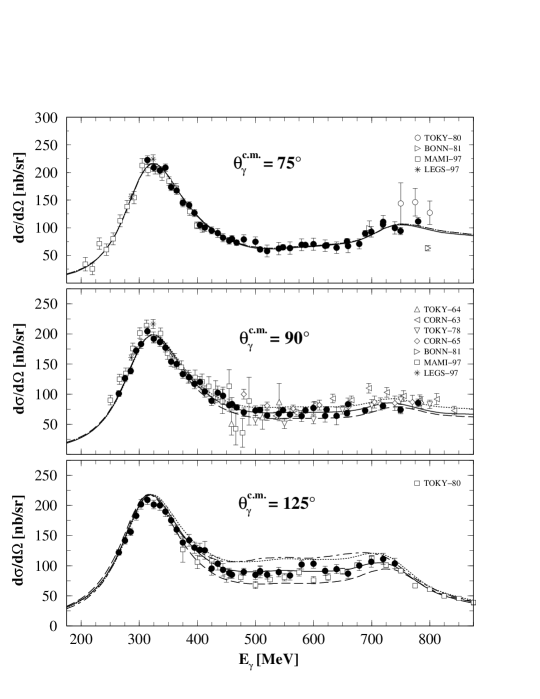
Figure 9: Differential cross sections for the first and second resonance region in comparison with data from other experiments. The curves show calculations based on the SAID-SM99K photo-meson amplitudes for $m_{\sigma}=400\;\mathrm{MeV}$ (dashed), $m_{\sigma}=600\;\mathrm{MeV}$ (solid) and $m_{\sigma}=800\;\mathrm{MeV}$ (dotted). Other parameters are those in Eq. (11). The dashed-dotted curve given for the angle 125^∘ shows calculations based on the MAID2K photo-meson amplitudes with $m_{\sigma}=$ 600 MeV and the other parameters specified in Eq. (12). The previous data are compiled in ukai97 and are taken from: ishii80 (TOKY-80); jung81 (BONN-81); huenger97 (MAMI-97); tonnison98 (LEGS-97); nagashima64 (TOKY-64); stiening63 (CORN-63); toshioka78 (TOKY-78); rust65 (CORN-65). The data of the present work (filled circles, representing angular intervals of $\Delta\theta^{c.m.}_{\gamma}=15^{\circ}$) are given with error bars taking into account the counting statistics, and systematic errors due to detection efficiency, geometrical uncertainties and background subtraction.

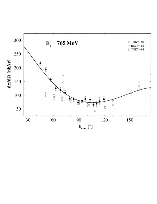
Figure 10: Differential cross sections for 765 MeV photon energy in comparison with data from other experiments. The curve shows a calculation based on the SAID-SM99K parameterization and on the parameters given in (11). The previous data are taken from: jung81 (BONN-81); ishii80 (TOKY-80); wada84 (TOKY-84). The data from the present work (⚫) represent energy intervals of $\Delta E_{\gamma}$ = 60 MeV width. Their error bars take into account the counting statistics and systematic errors due to detection efficiency, geometrical uncertainties and background subtraction.

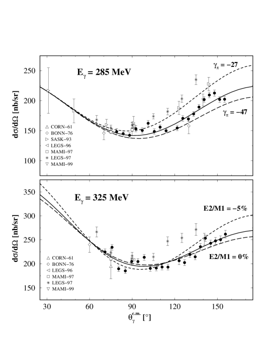
Figure 11: Angular distributions of Compton differential cross sections obtained with the LARA arrangement (filled circles, representing energy intervals of $\Delta E_{\gamma}=$ 40 MeV) compared with previous data as compiled in ukai97 and with predictions of dispersion theory with the SAID-SM99K photo-pion amplitudes. The full lines are obtained if the parameters of Eq. (11) are applied. The dashed lines show sensitivities to $\gamma_{\pi}$ at $E_{\gamma}=$ 285 MeV (upper part) and to the ratio E2/M1 at $E_{\gamma}=$ 325 MeV (lower part). The previous data are from: dewire61 (CORN-61); hallin93 (SASK-93); genzel76 (BONN-76); blanpied96 (LEGS-96); huenger97 (MAMI-97); tonnison98 (LEGS-97); wissmann99 (MAMI-99). The final value for the parameter $\gamma_{\pi}$ has not been obtained from these data points only but from the total amount of data below 455 MeV (see the text).

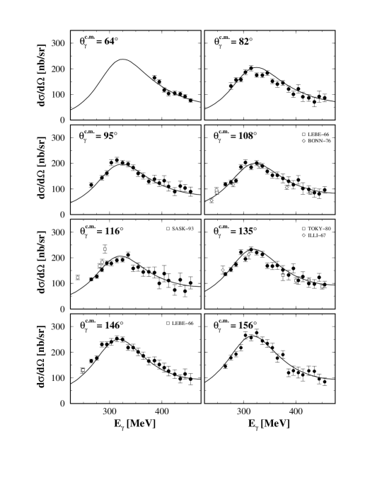
Figure 12: Eight out of 24 energy distributions from $59^{\circ}$ to $156^{\circ}$ (c.m.) obtained with the LARA arrangement in the first resonance range compared with previous data and with predictions from dispersion theory. The previous data are taken from: baranov66a ; baranov66b (LEBE-66); gray67 (ILLI-67); genzel76 (BONN-76); hallin93 (SASK-93); ishii80 (TOKY-80); the present work ($\bullet$) with error bars as in Fig. 9.

In Figs. 9–12 we discuss specific properties of our present experimental data in comparison with predictions and with previous results. Figs. 13–17 in the appendix show the complete set of data obtained in the present experiment compared with the same kind of predictions. As predictions we use the results of the dispersion theory lvov97 based on the SAID-SM99K parametrization of photo-meson amplitudes arndt96 together with the parameter $\alpha-\beta$, the difference of the electric and magnetic polarizability. For the latter quantity the global average $\alpha-\beta=(10.0\pm 1.5_{\mathrm{stat+syst}}\pm 0.9_{\mathrm{model}})\times 10^{-4}\;\mathrm{fm}^{3}$ has been obtained, taking into account experiments of 90’s macgibbon95 . More recently the LEGS group tonnison98 published the result $\alpha-\beta=10.11\pm 1.74_{\rm stat+syst}$ and the TAPS collaboration at MAMI (Mainz) obtained a new global average of $\alpha-\beta=10.5\pm 0.9_{\rm stat+syst}\pm 0.7_{\rm model}$ olmos01 .

The parameter $\alpha-\beta$ was not adjusted to the present data for two reasons: (i) This quantity is mainly due to a $t$-channel exchange and, therefore, essentially independent of the parametrization of photo-meson amplitudes. (ii) This quantity is strongly constrained by large-angle differential cross sections below pion photoproduction threshold where the present experiment made no contribution. The total photoabsorption cross section corresponding to the presently used parametrization leads through the Baldin sum rule to $\alpha+\beta=14.05\times 10^{-4}\;\mathrm{fm}^{3}$ and is in between the values of Babusci et al. babusci98 , being $\alpha+\beta=\left(13.69\pm 0.14\right)\times 10^{-4}\;\mathrm{fm}^{3}$, and $\alpha+\beta=\left(14.2\pm 0.3\right)\times 10^{-4}\;\mathrm{fm}^{3}$, which is based on numerical results of Ref. damashek70 . Some critical discussion of these and related numbers can be found in levchuk00 .

From the present data in the second resonance region the only remaining free parameter of the dispersion theory lvov97 , the effective mass-parameter of the $\sigma$ meson, was fitted leading to $m_{\sigma}=(589\pm 12_{\mathrm{stat+syst}})$ MeV with $\chi^{2}/{\rm d.o.f.}=1.33$ which essentially confirms the previous estimate lvov97 of $m_{\sigma}=600$ MeV. The procedure is illustrated in Fig. 9 where the three curves have been calculated with the effective mass parameters $m_{\sigma}$ =400, 600 and 800 MeV. This Figure as well as the corresponding data shown in Figs. 15-17 of the Appendix prove that the parametrization of the asymptotic part of the invariant aplitude $A_{1}(\nu,t)$ introduced in lvov97 is in line with the experimental data. The present and previous lvov97 result of $m_{\sigma}=600$ MeV is in agreement with what is frequently denoted as the “mass of a sigma meson”. However, we wish to stress here that we do not claim to have determined a “mass of a sigma meson”. For us this quantity merely is a number in the pole parametrization of the $t$-channel $J^{PC}=0^{++}$ exchange in the region of negative $t$ which leads to an excellent representation of the data of the second resonance region lvov97 . The data from the present and previous experiments shown in Fig. 9 are in a general good agreement with each other. Nevertheless, the improvement in accuracy achieved in the present experiment is quite apparent.

Systematic differences between present and previous data are seen in in Fig. 10 where the angular distribution of differential cross sections is shown for the photon energy E${}_{\gamma}=765$ MeV. Here the data from the Bonn-81 experiment jung81 are considerably below our data and below the predictions, especially in the forward direction. This shows that the coverage of the second resonance region through data from previous experiments was by far not sufficient.

After fixing the effective mass-parameter $m_{\sigma}$ to 600 MeV it is possible to use the differential cross-sections in the first resonance region up to 455 MeV photon energy to get information on two important quantities which were subject to several recent investigations. These are the backward spin polarizability $\gamma_{\pi}$ and the E2/M1 ratio of the $p\to\Delta$ transition. In accordance with previous work beck97a ; beck00 the $\mathrm{E2/M1}$ ratio is defined here as the ratio $\mbox{Im}E^{(3/2)}_{1+}/\mbox{Im}M^{(3/2)}_{1+}$ taken at the resonance point $E_{\gamma}=340$ MeV beck97a ; beck00 , where $\delta_{33}=90^{\circ}$ or, equivalently, $\mbox{Re}M^{(3/2)}_{1+}=0$. One can make a small change in the $\Delta$-resonance contribution to $M^{(3/2)}_{1+}$ or $E^{(3/2)}_{1+}$ and thus change the $\mathrm{E2/M1}$ ratio using a fine tuning of the $\Delta$-resonance photocouplings $(M_{1+}^{(3/2)})_{r}$ and $(E_{1+}^{(3/2)})_{r}$ as described elsewhere huenger97 . Such changes affect the imaginary part of the Compton scattering amplitude huenger97 and, through the dispersion relations, the real part too. A similar procedure may be applied to the backward spin polarizability $\gamma_{\pi}$ by adding an extra term to the asymptotic contribution $A_{2}^{\rm as}$ (7) usually represented only by the $\pi^{0}$-exchange tonnison98 . Such a change affects the real part of the Compton scattering amplitude only.

For a given $M_{1+}$ amplitude which essentially fixes the predicted differential cross sections at $\theta^{\mathrm{c.m.}}_{\gamma}=60^{\circ}$ and $115^{\circ}$, the E2/M1 ratio shows its highest sensitivity to the differential cross sections in the maximum of the $\Delta$-resonance and for $90^{\circ}$ and forward and backward angles. In practice this procedure gains its highest sensitivity if it is restricted to the subset of data between 280 and 360 MeV. The backward spin polarizability $\gamma_{\pi}$ shows its highest sensitivity to the differential cross sections for beam energies of about 285 MeV and only in the backward direction. In this case the evaluation may be caried out using all data below 455 MeV. The sensitivity of the data to the quantities $\gamma_{\pi}$ and E2/M1 is illustrated in the lower and upper parts of Fig.  11, respectively.

The overall quality of the data obtained in the present experiment for the first resonance region may be judged from Fig. 12 which shows selected examples of differential cross sections. There is a general good agreement with previous data with only few exceptions. This figure shows that in the $\Delta$ energy range the coverage with experimental differential cross sections is good except for small angles. The reason for this lack of data at small angles is that the recoil proton has a too low energy to leave the scattering target. In this range additional data may be measured using the large Mainz NaI(Tl) detector without recoil-proton detection.

In detail we used the following procedure to determine the multipoles characterizing the $\Delta$-resonance and to extract $\gamma_{\pi}$: We start with the fixed mass parameter $m_{\sigma}=600$ MeV and the new global average for the difference of the electric and magnetic polarizabilities of the proton olmos01 , $\alpha-\beta=(10.5\pm 0.9_{\rm stat+syst}\pm 0.7_{\rm model})\times 10^{-4}~{}\rm fm^{3}$ which nicely confirms the previous one macgibbon95 but with a reduced experimental error. Taking a subset of 167 data points close to the $\Delta$-resonance peak, namely those between the limits $E_{\gamma}=280$ and 360 MeV where the $\Delta$-resonance contribution strongly dominates, we slightly rescale the $\Delta$-resonance parts of the photo-pion amplitudes $M_{1+}$ and $E_{1+}$, as described in huenger97 , in order to achieve the best agreement between the present experimental data and dispersion-theory predictions. The above choice of the energy limits is made in order to reduce otherwise bigger model errors in the determination of the resonance parameters. With these corrected amplitudes, setting an overall scale for the theoretical differential cross sections of Compton scattering close to the resonance, we tune $\gamma_{\pi}$ through the asymptotic contribution to the invariant amplitude $A_{2}$ (7) in order to arrive at the best $\chi^{2}$ in the whole energy region covering the $\Delta$-resonance, which here is the region $E_{\gamma}\leq 455$ MeV containing 467 data points. With this $\gamma_{\pi}$ we repeat the determination of the amplitudes $M_{1+}$ and $E_{1+}$ and then arrive again at $\gamma_{\pi}$, etc. These iterations quickly converge and eventually give the final values for $M_{1+}$, $E_{1+}$ and $\gamma_{\pi}$.

In order to determine the model uncertainties of the extracted quantities we used different values for $\alpha-\beta$ within the experimental uncertainty of this quantity (i.e. between 9.4 and $11.6\times 10^{-4}~{}\rm fm^{3}$ olmos01 ). Also different values for $m_{\sigma}$ were used between 500 to 700 MeV. This range of $m_{\sigma}$ is supported by a comparison of different theoretical calculations of the amplitude $A_{1}$ lvov97 ; drechsel99 ; holstein94 ; lvov99a . Moreover, we varied the $\pi^{0}\gamma\gamma$ coupling by $\pm$4% and the $\eta NN$ and $\eta^{\prime}NN$ couplings by $\pm$50%. The form factors accompanying the $\pi^{0}$, $\eta$, $\eta^{\prime}$ $t$-channel contributions were varied and also the parameters which determine the multipole structure of double-pion photoproduction below 800 MeV where the latter variation was based on experience of a recent GDH experiment arends00 .

We present our findings in terms of the absolute value of the $M_{1+}^{(3/2)}$ amplitude at the energy 320.0 MeV corresponding to the maximum of the differential cross section for Compton scattering. The E2/M1 ratio (EMR) of the imaginary parts of the amplitudes $E_{1+}^{(3/2)}$ and $M_{1+}^{(3/2)}$ is determined for 340.0 MeV where the real parts of these amplitudes are about zero, in complete agreement with the previous procedure blanpied97 ; beck97a ; beck00 where the ratio of the imaginary parts was determined from pion photoproduction experiments. It is important to exactly use the same energy $E_{\gamma}$ when comparing the amplitudes $E_{1+}^{(3/2)}$ and $M_{1+}^{(3/2)}$ obtained from different experiments because they rapidly vary with $E_{\gamma}$. Our results are

$$|M_{1+}^{(3/2)}(320~{}{\rm MeV})| = (39.7\pm 0.3_{\rm stat+syst}\pm 0.03_{\rm model})$$

$$\times 10^{-3}/m_{\pi^{+}},$$

$${\rm EMR}(340~{}{\rm MeV}) = (-1.7\pm 0.4_{\rm stat+syst}\pm 0.2_{\rm model})\;\%,$$

$$\gamma_{\pi} = (-37.1\pm 0.6_{\rm stat+syst}\pm 3.0_{\rm model})$$ (11)

$$\times 10^{-4}~{}\rm fm^{4}.$$

The systematic errors given here include changes imposed by a simultaneous shift of all data points within the scale uncertainty of $\pm$3%. This uncertainty fully dominates the resulting uncertainty of the $M_{1+}^{(3/2)}$ amplitude. Note that the required modifications of the amplitudes $M_{1+}^{(3/2)}$ and $E_{1+}^{(3/2)}$ are compatible with zero. Without the modification, the SAID-SM99K parameterization gives
$|M_{1+}^{(3/2)}(320~{}{\rm MeV})|=39.74$ (in the same units) and
EMR$(340~{}{\rm MeV})=-1.68\%$. The present value for $M_{1+}^{(3/2)}$ perfectly agrees with the one previously determined by Hünger et al. huenger97 : $|M_{1+}^{(3/2)}(320~{}{\rm MeV})|=39.6\pm 0.4$. Since we did not try to tune other photo-meson amplitudes like $E_{0+}$, $M_{1-}$ or $E_{2-}$ which are also of importance for a good description of Compton scattering data near the $\Delta$-resonance, the model errors in (11) may still be incomplete.

The value of EMR determined from the present Compton scattering data is smaller than the one obtained in a dedicated Mainz photo-pion experiment, i.e. $(-2.5\pm 0.1_{\rm stat}\pm 0.2_{\rm syst})\%$ beck97a ; beck00 , and also smaller than the result published by the LEGS group blanpied97 , i.e. $(-3.0\pm 0.3_{\rm stat+syst}\pm 0.2_{\rm model})\%$. Our result essentially confirms the prediction of the SAID-SM99K parameterization, in agreement with the observation that this parameterization leads to an overall agreement with our Compton scattering differential cross sections. However, it should be noted that by applying the same procedure as before but fixing the E2/M1 ratio to EMR(340 MeV)=$-2.5\%$, a good fit to our data in the $\Delta$ resonance region may also be obtained with only slight shifts in the parameters $M_{1+}^{(3/2)}(320~{}{\rm MeV})$ and $\gamma_{\pi}$. Therefore, at this stage of the investigation we do not contribute to the extensive discussion of the E2/M1 ratio beck97b ; beck97c ; davidson97 ; workman97 carried out in the past.

The uncertainties of the spin polarizability $\gamma_{\pi}$ are dominated by the model errors, especially – for a given choice of photo-meson amplitudes – by the variations of $m_{\sigma}$ and $\alpha-\beta$. Taking these into account our result for $\gamma_{\pi}$ is in disagreement with the one determined in 1997 by the LEGS group tonnison98 which gave the smaller value $\gamma_{\pi}^{\rm LEGS}=-27.1\pm 2.2_{\rm stat+syst}{{}^{+2.8}_{-2.4}}{}_{\rm model}$ (in the same units of $10^{-4}~{}\rm fm^{4}$). This difference can be traced back to a difference in the measured differential cross sections, as can be seen in Fig. 11. The former result tonnison98 is also in contradiction to standard dispersion theory drechsel98 ; babuscu98a ; lvov99 and also to chiral perturbation theory hemmert98 ; gellas00 ; kumar00 . As a consequence is was concluded that hitherto unknown effects related to the spin structure of the nucleon might exist. With our new data such effects are clearly ruled out, in accordance with our recently published data on quasi-free scattering from the proton wissmann99 and with the one obtained very recently by the TAPS collaboration at MAMI olmos01 , i.e. $\gamma_{\pi}=-36.1\pm 2.1_{\rm stat}\mp 0.4_{\rm syst}\pm 0.8_{\rm model}$.

The present value of $\gamma_{\pi}\approx-37.1$ agrees well with predictions of the unsubtracted dispersion relation for the invariant amplitude $A_{2}$ adopted in lvov97 . The latter gives $-38.24$ with the same photo-meson input and with the same energy cut in the dispersion integrals of $E_{\rm max}=1.5$ GeV, thus assuming no essential asymptotic contributions beyond pseudoscalar-meson exchanges ($\pi^{0},\eta,\eta^{\prime}$). The present value for $\gamma_{\pi}$ satisfactorily agrees with predictions of the “small scale expansion” scheme, which effectively is chiral perturbation theory including the $\Delta$-resonance, $\gamma^{\rm SSE}_{\pi}=-37$ hemmert98 . It also agrees with standard chiral perturbation theory to order $O(p^{4})$, which does not include the $\Delta$-resonance, $\gamma^{\rm ChPT}_{\pi}=-39$ kumar00 , provided $-45$ is used for the anomaly contribution to $\gamma_{\pi}$ from $\pi^{0}$ exchange. Furthermore, it agrees with backward-angle dispersion relations, which include the $\Delta$ and the $\eta$-$\eta^{\prime}$ exchanges, $\gamma^{\rm DR}_{\pi}=-39.5\pm 2.4$ lvov99 . Thus, there is good overall consistency between the present Compton scattering data, the dispersion theory, and the SAID-SM99K photo-meson amplitudes.

Such a consistency is deteriorated when the latest SAID-SM00K photo-pion amplitudes are used. This is because in that latest parameterization the $M1$-strength of the $\Delta$-resonance is decreased to $|M_{1+}^{(3/2)}(320~{}{\rm MeV})|=39.16$. Therefore, we have to increase the SM00K $M_{1+}{(3/2)}$- amplitude by $+1.2\%$ in order to achieve a satisfactory description of Compton scattering. When such a rearrangement is made, the value extracted for $\gamma_{\pi}$ is $\gamma_{\pi}=-37.0$, i.e. it turns out to be only slightly smaller than the one of Eq.(1) with similar errors.

When using the MAID2K maid parameterization of photo-pion amplitudes the same procedure gives the results

$$|M_{1+}^{(3/2)}(320~{}{\rm MeV})| = (39.8\pm 0.3_{\rm stat+syst}\pm 0.03_{\rm model})$$

$$\times 10^{-3}/m_{\pi^{+}},$$

$${\rm EMR}(340~{}{\rm MeV}) = (-2.0\pm 0.4_{\rm stat+syst}\pm 0.2_{\rm model})\;\%,$$

$$\gamma_{\pi} = (-40.9\pm 0.4_{\rm stat+syst}\pm 2.2_{\rm model})$$ (12)

$$\times 10^{-4}~{}\rm fm^{4}$$

which are more at variance with Eq. (11) than the alternatives discussed above. In this case a slightly bigger rearrangement of the resonance amplitudes is required in comparison with their original values which, for MAID2K, are $|M_{1+}^{(3/2)}(320~{}{\rm MeV})|=39.92$ and EMR$(340~{}{\rm MeV})=-2.19\%$. The biggest change is, however, in the spin polarizability $\gamma_{\pi}$ which can be traced back to rather different nonresonant amplitudes $E_{0+}$ and $E_{2-}$ in the SAID and MAID representations in the $\Delta$-resonance range. The overall quality of the description of the present Compton scattering data at energies below 455 MeV, containing 467 data points in total, is approximately the same for the SAID and MAID photo-meson input. The fitting procedure based on the two sets of parameterizations leads to $\chi^{2}=564$ in both cases and the differences in the predictions are small as can be seen in Fig. 9.

However, the properties of the SAID and MAID parameterizations are quite different in the second resonance region. For instance, $\chi^{2}/{\rm d.o.f.}=1.36$ is obtained for all data point above 455 MeV for the SAID-based theoretical predictions with SAID-based parameters (1), whereas $\chi^{2}/{\rm d.o.f.}=2.00$ is obtained for the same data points with MAID-based theoretical predictions and MAID-based parameters (2). This means that the MAID-based parameterization does not lead to a reasonable fit to the data when the same parameter $m_{\sigma}=600$ MeV is used. The biggest difference between these two versions is seen at backward angles in the dip region between the first and second nucleon resonance, as illustrated by the dashed-dotted curve in Fig. 9. The use of a smaller $m_{\sigma}$ with the same $\gamma_{\pi}$ reduces the discrepancy in the dip region, however without leading to an overall agreement. It is observed that the fit to the data below 455 MeV carried out with that smaller $m_{\sigma}$ requires an even bigger $-\gamma_{\pi}$ compared to the one given in (2), and with this bigger $-\gamma_{\pi}$ again no agreement is achieved between the theory and the data in the dip region.

6 Conclusions

The results of the present experiment may be summarized as follows. For the first time Compton scattering by the proton has been measured with a large acceptance set-up for the scattering angle and the photon energy. The data confirm the magnitude of the $M1$-strength adopted in the SAID-SM99K and MAID2K parameterizations (not in SAID-SM00K), and are in agreement with the E2/M1 ratio given by these parameterizations. The backward spin polarizability $\gamma_{\pi}$ is found to be in agreement with latest theoretical calculations, although model errors should yet be better understood.

References

- (1) P.S. Baranov, L.V. Fil’kov, Sov. J. Part. Nucl. 7, (1976) 42
- (2) V.A. Petrun’kin, Sov. J. Part. Nucl. 12, (1981) 278
- (3) H. Genzel, M. Jung, R. Wedemeyer, H.J. Weyer, Z. Physik A 279, (1976) 399
- (4) M. Jung, J. Kattein, H. Kück, P. Leu, K.-D. de Marné, R. Wedemeyer, N. Wermes, Z. Physik C 10, (1981) 197
- (5) T. Ishii, E, Egawa, S. Kato et al., Nucl. Phys. B 165, (1980) 189
- (6) Y. Wada, K. Egawa, A. Imanishi et al., Nucl. Phys. B 247, (1984) 313
- (7) E.L. Hallin et al. Phys. Rev. C 48, (1993) 1497
- (8) G. Blanpied et al., Phys. Rev. Lett. 76, (1996) 1023
- (9) G. Blanpied et al., Phys. Rev. Lett. 79, (1997) 4337
- (10) J. Tonnison et al., Phys. Rev. Lett. 80, (1998) 4382; G. Blanpied et al., Phys. Rev. C 64, (2001) 025203
- (11) J. Peise et al., Phys. Lett. B 384, (1996) 37
- (12) A. Hünger et al., Nucl. Phys. A 620, (1997) 385
- (13) F. Wissmann et al., Nucl. Phys. A 660, (1999) 232
- (14) C. Molinari et al., Phys. Lett. B 371, (1996) 181
- (15) H. Falkenberg, J. Ahrens, G.P. Capitani et al., Nucl. Inst. Meth. A 360, (1995) 559
- (16) W. Pfeil, H. Rollnik, S. Stankowski, Nucl. Phys. B 73, (1974) 166
- (17) I. Guiasu, C. Pomponiu, E.E. Radescu, Ann. Phys. (N.Y.) 114, (1978) 296
- (18) D.M. Akhmedov, L.V. Fil’kov, Sov. J. Nucl. Phys. 33, (1981) 573
- (19) A.I. L’vov, Sov. J. Nucl. Phys. 34, (1981) 597
- (20) A.I. L’vov, Sov. J. Nucl. Phys. 42, (1985) 583
- (21) A.I. L’vov, V.A. Petrun’kin, M. Schumacher, Phys. Rev. C 55, (1997) 359
- (22) G. Hida, M. Kikugawa, Progr. Theor. Phys. 55, (1976) 1156; 58, (1977) 372
- (23) T. Feuster, U. Mosel, Phys. Rev. C 59, (1999) 460
- (24) A.Yu. Korchin, O. Scholten, R.G.E. Timmermans, Phys. Lett. B 438, (1998) 1
- (25) A.Yu. Korchin, O. Scholten, Phys. Rev. C 62, (2000) 015205
- (26) D. Drechsel et al., Phys. Rev. C 61, (1999) 015204
- (27) R.A. Arndt, I.I. Strakovsky, R.L. Workman, Phys. Rev. C 53, (1996) 430
- (28) D. Drechsel et al., Nucl. Phys. A 645 (1999) 145; http://www.kph.uni-mainz.de/MAID
- (29) G. Galler et al., Phys. Lett. B 503 (2001) 245
- (30) I. Anthony et al., Nucl. Instr. Meth. A 301, (1991) 230; S.J. Hall et al., Nucl. Instr. Meth. A 368, (1996) 698
- (31) H. Herminghaus et al., Nucl. Instr. Meth. 138, (1976) 1; A 187, (1981) 103
- (32) P. Grabmayr et al., Nucl. Instr. Meth, A 402, (1998) 85
- (33) A.I. L’vov, A.M. Nathan, Phys. Rev. C 59, (1999) 1064
- (34) B. E. MacGibbon et al., Phys. Rev. C 52, (1995) 2097
- (35) P.S. Baranov, A.I. L’vov, V.A. Petrun’kin, L.N. Shtarkov, 9th International Seminar on Electromagnetic Interactions of Nuclei at Low and Medium Energies, Moscow, Russia, 20-22 Sep 2000 nucl-ex/0011015
- (36) V. Olmos de León et al., Eur. Phys. J. A 10, (2001) 207
- (37) D. Babusci, G. Giordano, G. Matone, Phys. Rev. C 57, (1998) 291
- (38) M. Damashek, F.J. Gilman, Phys. Rev. D 1, (1970) 1319
- (39) M.I. Levchuk, A.I. L’vov, Nucl. Phys. A 674, (2000) 449
- (40) K. Ukai, T. Nakamura, Data Compilation of Single Pion Photoproduction below 2 GeV, INS-T-550 (1997)
- (41) Y. Nagashima et al., PRP Institute for Nuclear Study, University of Tokyo 81, (1964)
- (42) R. F. Stiening, E. Loh, M. Deutsch, Phys. Rev. Lett. 10, (1963) 536
- (43) K. Toshioka et al., Nucl. Phys. B 141, (1978) 364
- (44) D.R. Rust et al., Phys. Rev. Lett. 15, (1965) 938
- (45) R. Beck et al., Phys. Rev. Lett. 78, (1997) 606
- (46) R. Beck et al., Phys. Rev. C 61, (2000) 035204
- (47) B.R. Holstein, A.M. Nathan, Phys. Rev. D 49 (1994) 6101
- (48) A.I. L’vov, A.M. Nathan, unpublished (1999)
- (49) H.-J. Arends (private communication)
- (50) J.W. DeWire et al., Phys. Rev. 124, (1961) 909
- (51) P.S. Baranov et al., JETP 23, (1966) 242
- (52) P.S. Baranov et al., Sov. J. Nucl. Phys. 3, (1966) 3 791
- (53) E.R. Gray, A.O. Hanson, Phys. Rev. 160, (1967) 1212
- (54) R. Beck and H.P. Krahn, Phys. Rev. Lett. 79, (1997) 4510
- (55) R. Beck and H.P. Krahn, Phys. Rev. Lett. 79, (1997) 4512
- (56) R.M. Davidson and N.C. Mukhopadhyay, Phys. Rev. Lett. 79, (1997) 4509
- (57) R.L. Workman, Phys. Rev. Lett. 79, (1997) 4511
- (58) D. Drechsel, G. Krein, O. Hanstein, Phys. Lett. B 420, (1998) 248
- (59) D. Babusci, G. Giordano, A.I. L’vov, G. Matone, A.M. Nathan, Phys. Rev. C 58, (1998) 1013
- (60) T.R. Hemmert, B.R. Holstein, J. Kambor, G. Knöchlein, Phys. Rev. D 57, (1998) 5746
- (61) G.C. Gellas, T.R. Hemmert, U.-G. Meissner, Phys. Rev. Lett. 85, (2000) 14
- (62) K.B. Vijaya Kumar, J.A. McGovern, M.C. Birse, Phys. Lett. B479 (2000) 167
- (63) M.C. Birse, X. Ji, J.A. McGovern, Phys. Rev. Lett. 86 (2001) 3204